Preprint
Article

This version is not peer-reviewed.

Artificial Intelligence for Multiclass Rhythm Analysis for Out-of-Hospital Cardiac Arrest During Mechanical Cardiopulmonary Resuscitation

A peer-reviewed article of this preprint also exists.

Submitted:

05 March 2025

Posted:

07 March 2025

You are already at the latest version

Abstract

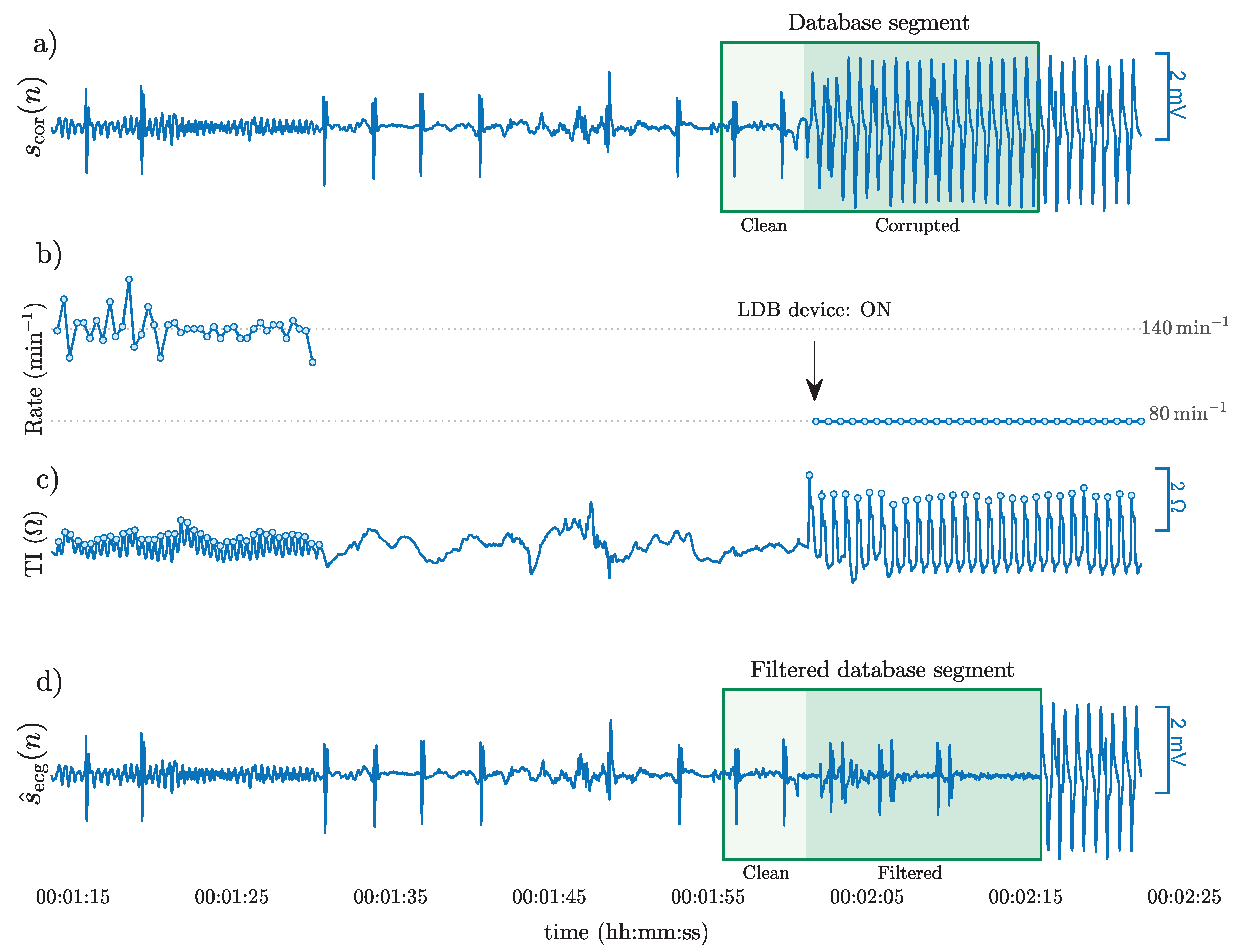
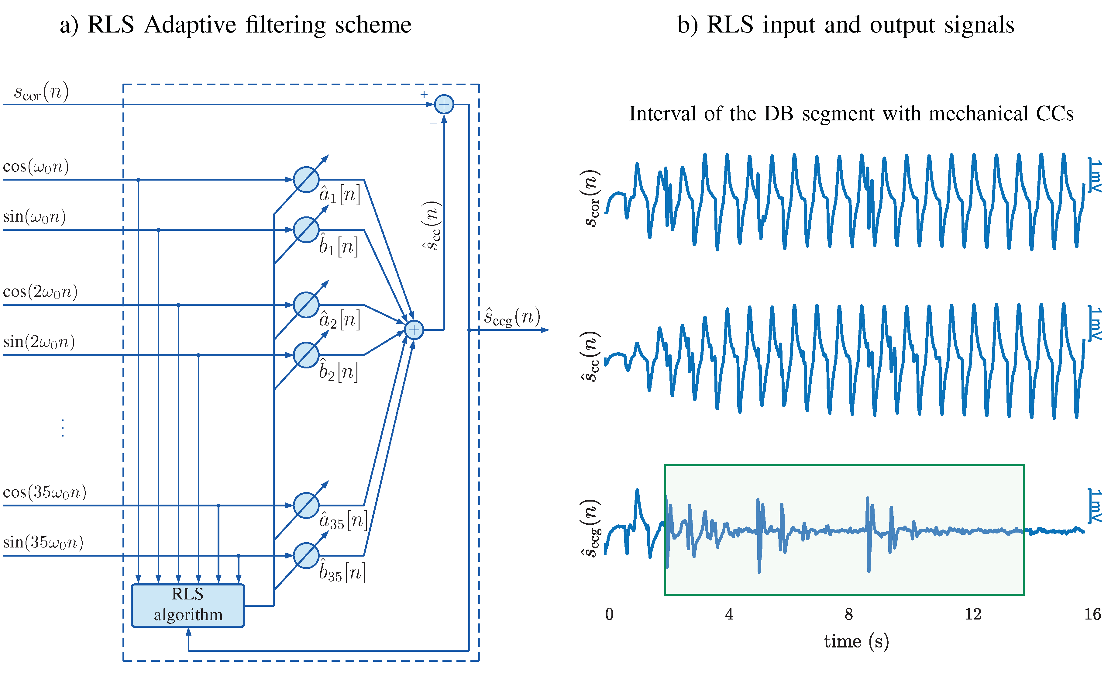
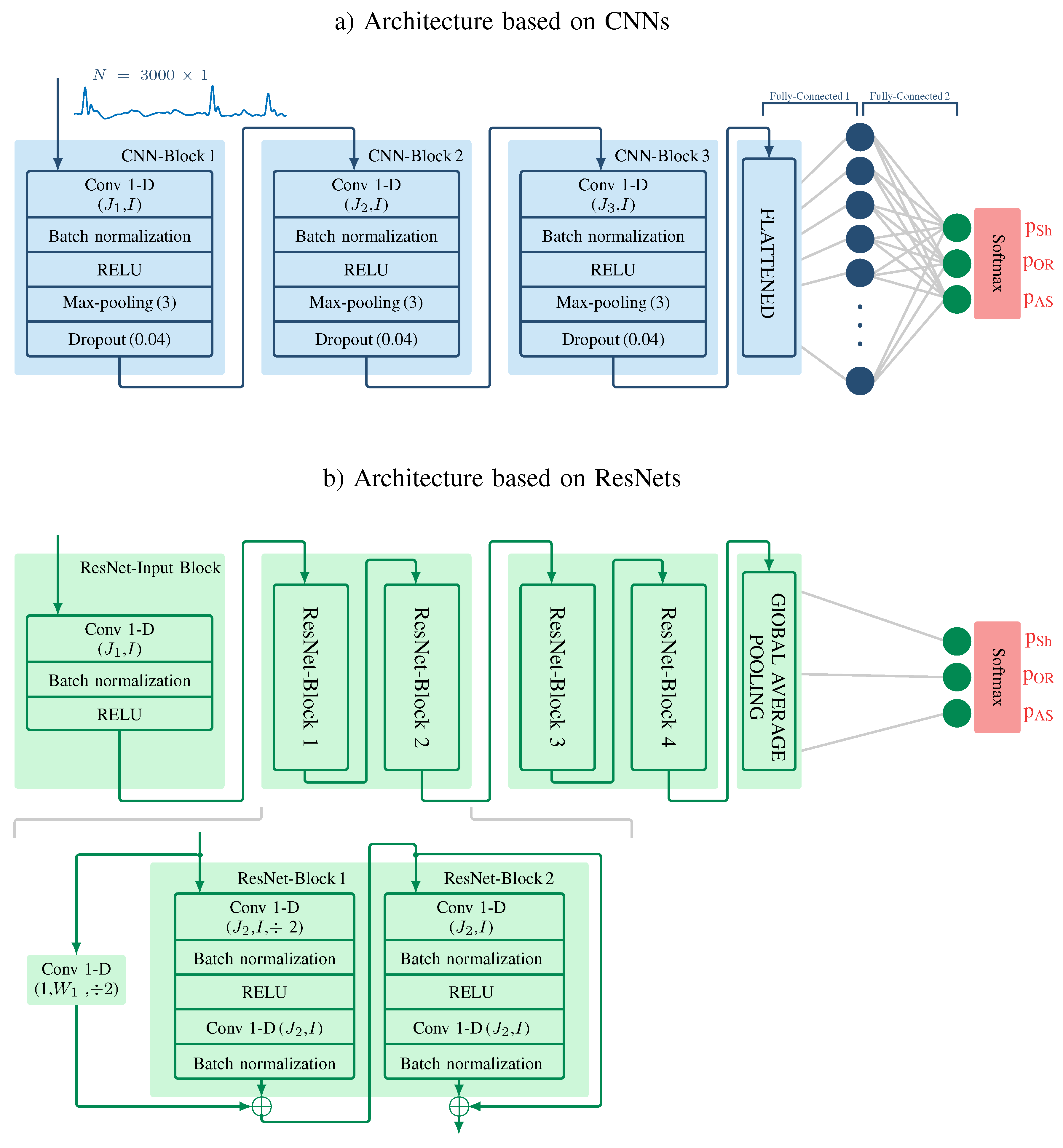
Load Distributing Band (LDB) mechanical chest compression (CC) device is used to treat out-of-hospital cardiac arrest (OHCA) patients. Mechanical CCs induce artifacts in the electrocardiogram (ECG) recorded by defibrillators, potentially leading to inaccurate cardiac rhythm analysis. A reliable analysis of the cardiac rhythm is essential for guiding resuscitation treatment and understanding retrospectively patients’ response to treatment. The aim of this study was to design an artificial intelligence (AI)-based framework for cardiac automatic multiclass rhythm classification in the presence of CC artifacts during OHCA. Concretely, an automatic multiclass cardiac rhythm classification is addressed to distinguish the following types of rhythms: shockable rhythms (Sh), asystole (AS) and organized rhythms (OR). A total of 15479 segments (2406 Sh, 5481 AS, 7592 OR) were extracted from 2058 patients during LDB CCs, whereof 9666 were used to train the algorithms and 5813 to assess the performance. The proposed architecture consisted of an adaptive filter for CC artifact suppression and a multiclass rhythm classifier. Three alternatives were considered for the multiclass classifier: a traditional machine learning algorithm and two deep-learning architectures based on convolutional neuronal networks and residual networks (ResNets). The unweighted mean of sensitivities, unweighted mean of bad hbox and the accuracy of the best method (ResNets) were 88.3%, 88.3% and 88.2%, respectively. These results highlight the potential of AI-based methods to provide accurate cardiac rhythm diagnoses without interrupting mechanical CC therapy.

Keywords: 
;  ;  
Subject: 
Engineering  -   Bioengineering

1. Introduction

Out-of-hospital cardiac arrest (OHCA) is one of the leading causes of death worldwide, with an annual incidence of 67 to 170 per 100 000 inhabitants in Europe and survival rates at hospital discharge of around 8% (0% to 18%) [1]. OHCA survival depends on several crucial factors, including bystander cardiopulmonary resuscitation (CPR) with emphasis on chest compresions (CCs), early defibrillation and the overall standard of medical care provided by the emergency medical services (EMS) [2].
Recognizing the patient’s cardiac rhythm throughout resuscitation is crucial for two key reasons: first, to guide therapy according to the treatment pathways defined by the international guidelines; and second, to retrospectively analyze the patient’s response to treatment. Regarding the first case, resuscitation guidelines emphasize the need of discriminating between shockable (Sh) rhythms, comprising ventricular fibrillation (VF) and pulseless ventricular tachycardia (VT), and non-shockable (NSh) rhythms, which include both organized rhythms (OR) and asystole (AS). The Sh/NSh discrimination is the most crucial decision during resuscitation, as defibrillation is the only treatment capable of restoring the normal function of the heart when a Sh rhythm is present [2,3]. A finer classification of the cardiac rhtyhm may also be needed, especially within the NSh rhyhm group, to determine other decisive therapies. For instance, the recommended treatment for AS consists of high-quality CPR, early administration of adrenaline and identification of the underlying cause of the arrest [4], whereas the presence of an OR could be an indicative of the return of spontaneous circulation, in which case the patient should be transported to hospital for post-resuscitation care and recovery [2]. As for the restrospective debriefing of resuscitation episodes, knowledge of the patient’s rhythm throughout the episode may offer valuable insights on the interaction between therapy and physiological response [5,6,7]; this may help identify optimal treatment strategies or clinical interventions that improve OHCA survival. One of the limitations for such retrospective studies is the lack of OHCA databases including cardiac rhythm annotations by expert clinicians, mostly due to the expensive and time-consuming manual labor required. Given all this, there is a clear need for the development of multiclass algorithms that automatically identify the patient’s cardiac rhythm, both in real time and retrospectively.
The state-of-the-art OHCA rhythm classification algorithms are mainly based on the analysis of the ECG, typically consisting of an ECG feature extraction stage followed by a machine learning (ML) classifier. They mostly consist of an ECG feature extraction stage followed by a ML classifier. ECG feature extraction has been approached in time [8,9], frequency [10,11], combined time-frequency [12] and complexity domains [13,14]. The ML approaches explored for the classification stage include K-nearest neighbors [15,16], support vector machines [17,18], artificial neural networks [19] and ensembles of decision trees [20]. Recently, OHCA rhythm classifcation has shifted towards deep learning (DL) techniques, such as convolutional neural networks (CNN) [21,22] or residual networks (ResNet) [23] that avoid the knowledge-based feature extraction process of traditional ML models. As determining the need for defibrillation is crucial in OHCA, the discrimination between Sh and NSh rhythms has been the most commonly addressed classification problem by the aforementioned algorithms. However, a less simplistic cardiac rhythm classification is needed to determine other decisive therapies during CPR [24,25,26]. To address this, Rad et al. [16] introduced the first multiclass OHCA rhythm classifier, where a set of features derived from the discrete wavelet analysis of the ECG were fed into different ML-based classifiers.
These ML and DL-based binary and multiclass algorithms have primarily focused on rhythm classification during interruptions in chest compressions (CCs), as the mechanical activity during CPR introduces ECG artifacts that hinder accurate rhythm detection. As a result, current commercial defibrillators require rescuers to pause CCs every 2 minutes for rhythm analysis. However, these interruptions reduce blood flow to vital organs, decreasing the chances of survival [27]. Over the past few decades, efforts have been made to develop more accurate rhythm analysis algorithms that could be applied during CCs, and thus help minimize CC interruptions [10,28]. These algorithms typically follow a similar structure to those used during non-CC intervals, but include a preliminar filtering step to remove CC-induced artifacts. Such methods have proven successful in classifying both Sh/NSh and multiclass rhythms during OHCA [29,30,31].
While earlier methods primarily focused on manually delivered CCs, the use of mechanical compression devices in OHCA assistance has notably increased. These devices provide CCs at a constant rate and depth, and although evidence supporting improved survival remains inconclusive [32,33,34], their growing adoption underscores the potential benefits they offer. Mechanical devices help ensure the quality of CCs in line with current resuscitation guidelines, even in situations where manual CPR might be compromised, such as during transport [35,36], in confined spaces, or during prolonged resuscitation efforts when rescuer fatigue may impact performance [37]. In addition, these devices alleviate the physical burden on healthcare providers, allowing them to focus on other aspects of patient care. While some proposals have addressed the Sh/NSh rhythm classification in the context of mechanical CCs [38,39,40], no solutions have yet been developed for multiclass rhythm classification.
This study introduces a robust ML/DL framework for a reliable multiclass classification of the cardiac rhythm to distinguish Sh, AS or OR rhythms during mechanical CPR. Both DL and ML architectures are preceded by an adaptive filtering stage to remove mechanical CC artifacts from the ECG. The ML framework includes a feature extraction stage and a random forest (RF) classifier. In the DL framework, the filtered ECG is directly analyzed using CNN- and ResNet-based classification models.

2. Materials

The data used in this study were collected from the Circulation Improving Resuscitation Care (CIRC) trial designed to compare automated load distributing band CPR (LDB-CPR) with high-quality manual CPR (M-CPR), in terms of survival [32,41]. Data were gathered between March 5, 2009 and January 11, 2011 in a randomized, unblinded, controlled group sequential trial of OHCA patients by three US (Fox Valley, Hilsborough, Houston) and two European (Vienna, Nijmegen) EMS. After EMS providers initiated manual CCs, patients were randomized to receive either LDB-CPR or M-CPR. The LDB device (AutoPulse, ZOLL Medical, Chelmsford, MA, USA) delivered CCs in a fixed position, with constant depth of 20% of the patient’s anterior posterior diameter of the chest and at a constant rate of 80 min -1 ( f LDB = 1.33   Hz ).
Anonymized data from Lifepak 12 and 15 monitor-defibrillators were exported to Matlab (MathWorks Inc., Natick, MA), using Physio-Control’s CODE-STAT data review software, and resampled to a sampling frequency of 250 Hz. The data included the ECG and thoracic impedance (TI) signals of each episode together with the CC instants detected by the CODE-STAT software. Figure 1 corresponds to a 70 s interval from an OHCA episode showing the ECG (corrupted by CCs) and TI signals in the panels a) and c), respectively. The blue circles on the TI signal indicate the CC instants detected by the CODE-STAT software. As can be seen, each fluctuation in the TI signal corresponds to a CC administered by the EMS. So, in Figure 1, two series of CCs can be clearly distinguished in the 0 15   s and 47 70   s time intervals corresponding to M-CPR and LDB-CPR, respectively. The middle interval, from 15 s to 47 s , corresponds to a segment without CCs and therefore free of CC artifacts. Note the clear difference in the TI pattern during LDB-CPR and M-CPR, with much larger amplitude and a more regular pattern for LDB-CPR due to the constant depth and rate of the mechanical CCs. The panel b) of Figure 1 shows the instantaneous CC rate derived from the CC instants marked in panel c). It can be observed that the CC rate for manual CPR was variable and fluctuated around 140 min -1, but when the LDB device was applied the CC frequency stabilized in 80 min -1.
Episodes where LDB-CPR was administered were used to conduct this study and the application of the LDB device was identified when the CC rate stabilized at the device’s fixed rate of 80 min -1 for at least 20 s (notice the activation of the LDB device in panel b) of Figure 1). Then, 22 s signal segments were extracted, corresponding to a single cardiac rhythm, and comprising a 6 s CC-free interval and a 16 s corrupted by CC artifacts (refer to the highlighted segment in Figure 1). The intervals during CCs were used as inputs for the multiclass decision algorithms, while the artifact-free intervals were employed to annotate the real underlying rhythm of the patient. Rhythms were annotated as Sh, AS or O.R. The segments corresponding to the EMS of Hilsborough, Nijmegen and Vienna were annotated by consensus of three biomedical engineers and subsequently audited by a clinician specialized in the resuscitation field. These segments were used to evaluate the performance of the multiclass decision algorithms. The segments corresponding to the remaining two EMS were not audited by a clinician and were therefore used to train the algorithms.
The final database consisted of 15479 segments extracted from 2058 patients, whereof 9666 segments (1252 Sh, 3865 AS, 4549 OR) from 1178 patients were used to train/develop the multiclass decision algorithms and 5813 segments (1154 Sh, 1616 AS, 3043 OR) from 880 patients were used to test the performance.

3. Methods

This study proposes and evaluates different algorithms for the three-class (Sh, AS, OR) classification of ECG segments corrupted by LDB CC artifacts. All the algorithms were composed of two main stages: 1) an adaptive filter based on a Recursive Least Squares (RLS) to eliminate CC artifacts from the ECG and 2) a classification stage, for which RF, CNN and ResNet models were optimized to classify the rhythm in the filtered ECG as Sh, AS or OR. All the classification models were designed to analyze the filtered ECG in the interval from 2-14 s (see the highlighted interval in Figure 2) which may help avoid the filtering transients of the RLS filter. In what follows t = n · T s , where T s = 4 m s is the sampling period ( f s = 250 Hz ), and n is the sample index.

3.1. CPR Artifact Suppressing Filter

During CPR, the corrupted ECG signal, s cor ( n ) , recorded by the defibrillator, can be expressed as
s cor ( n ) = s ecg ( n ) + s cc ( n ) ,
where s ecg ( n ) is the patient’s uncorrupted ECG, reflecting the actual underlying heart rhythm and, s cc ( n ) represents the artifact introduced by CCs.
An adaptive RLS filter, tailored for removing periodic interferences [38,42,43],was used to obtain an estimate of the CC artifact s ^ cc ( n ) , which was then substracted from s cor ( n ) to obtain the filtered ECG s ecg ( n ) , i.e an estimate of the true underlying heart rhythm. In this approach, the artifact is assumed to be quasi-periodic, and modeled as a truncated Fourier series of N terms:
s cc ( n ) = k = 1 N c k ( n ) cos ( k ω 0 n + θ k ( n ) ) = k = 1 N a k ( n ) cos ( k ω 0 n ) + b k ( n ) sin ( k ω 0 n ) ,
where ω 0 is the fundamental discrete frequency of CCs which for a LDB device is constant at ω 0 = 2 π f LDB T s with f LDB = 1.33 Hz 80 min 1 and T s the sampling period. Based on this model, the estimated artifact can be expressed in vector format as
s ^ cc ( n ) = Θ T ( n 1 ) Φ ( n ) ,
where vectors Θ ( n ) and Φ ( n ) , respectively, define the time-varying coefficients and the in-phase and quadrature reference signals of the Fourier series:
Θ ( n ) = [ a 1 ( n ) b 1 ( n ) a N ( n ) b N ( n ) ] T
Φ ( n ) = [ cos ( ω 0 n ) sin ( ω 0 n ) cos ( N ω 0 n ) sin ( N ω 0 n ) ] T
The RLS filter estimates the a k ( n ) and b k ( n ) coefficients adaptively over time so that the error between the corrupted ECG, s cor ( n ) , and the estimated artifact, s ^ cc ( n ) , is minimized at each iteration at the harmonics of the LDB device compression frequency, f LDB . Note that in this configuration (Figure 2), the error signal corresponds to the filtered ECG, s ^ ecg ( n ) . The update equations of the filter are given by
s ^ ecg ( n ) = s cor ( n ) s ^ cc ( n )
F ( n ) = 1 λ F ( n 1 ) F ( n 1 ) Φ ( n ) Φ T ( n ) F ( n 1 ) λ + Φ T ( n ) F ( n 1 ) Φ ( n )
Θ ( n ) = Θ ( n 1 ) + F ( n ) Φ ( n ) s ^ ecg ( n ) ,
where the gain matrix, F ( n ) , and the coefficient vector were initialized to F ( 0 ) = 0.03 I 2 N and Θ ( 0 ) = 0 T . As shown in the previous equations, there are two configurable parameters in the RLS filter: the number of harmonics, N, that model the artifact, and the forgetting factor, λ , which provides a trade-off between the filter’s adaptability and stability. These values were fixed to N = 35 and λ = 0.989 , based on the optimal RLS configuration identified in [39], where the RLS filter was evaluated in terms of the performance of a Sh/NSh decision algorithm applied to the filtered signal. Panel a) of Figure 2 shows the adaptive RLS filtering schema, while panel b) displays the input and output signals, from top to bottom: the corrupted ECG, s cor ( n ) , the estimated CC artifact, s ^ cc ( n ) , and the filtered ECG revealing the underlying rhythm of the patient, which in this case corresponds to an OR rhythm.

3.2. Optimization and Evaluation

The training set, composed of 9666 segments derived from 1178 patients, was used in a 10-fold cross validation (CV) approach for hyperparameter optimization and, in the case of RF models, for feature selection; details on the hyperparameters and feature selection are provided in the upcoming sections corresponding to each model. Data were divided patient-wise and ensuring that every fold retained a prevalence of each rhythm comparable to that of the entire dataset.
The remaining 5813 segments, corresponding to 880 patients, were used to evaluate the performance of the classifiers. For each class i Sh , AS , OR , the sensitivity ( Se i ), positive predictive value ( PPV i ) and F1-Scorei were computed, and the unweighted mean of all sensitivities (UMS), total accuracy (ACC) and unweighted mean of all F1-Scores (UMFS) were used as summarizing metrics:
Se i = TP i TP i + FN i , PPV i = TP i TP i + FP i , F 1 - Score i = 2 · PPV i · Se i PPV i + Se i UMS = 1 3 i = 1 3 Se i , ACC = TP + TN TP + TN + FP + FN , UMFS = 1 3 i = 1 3 F 1 - Score i
where TP i , TN i , FP i and FN i are the true positives, true negatives, false positives and false negatives for class i.

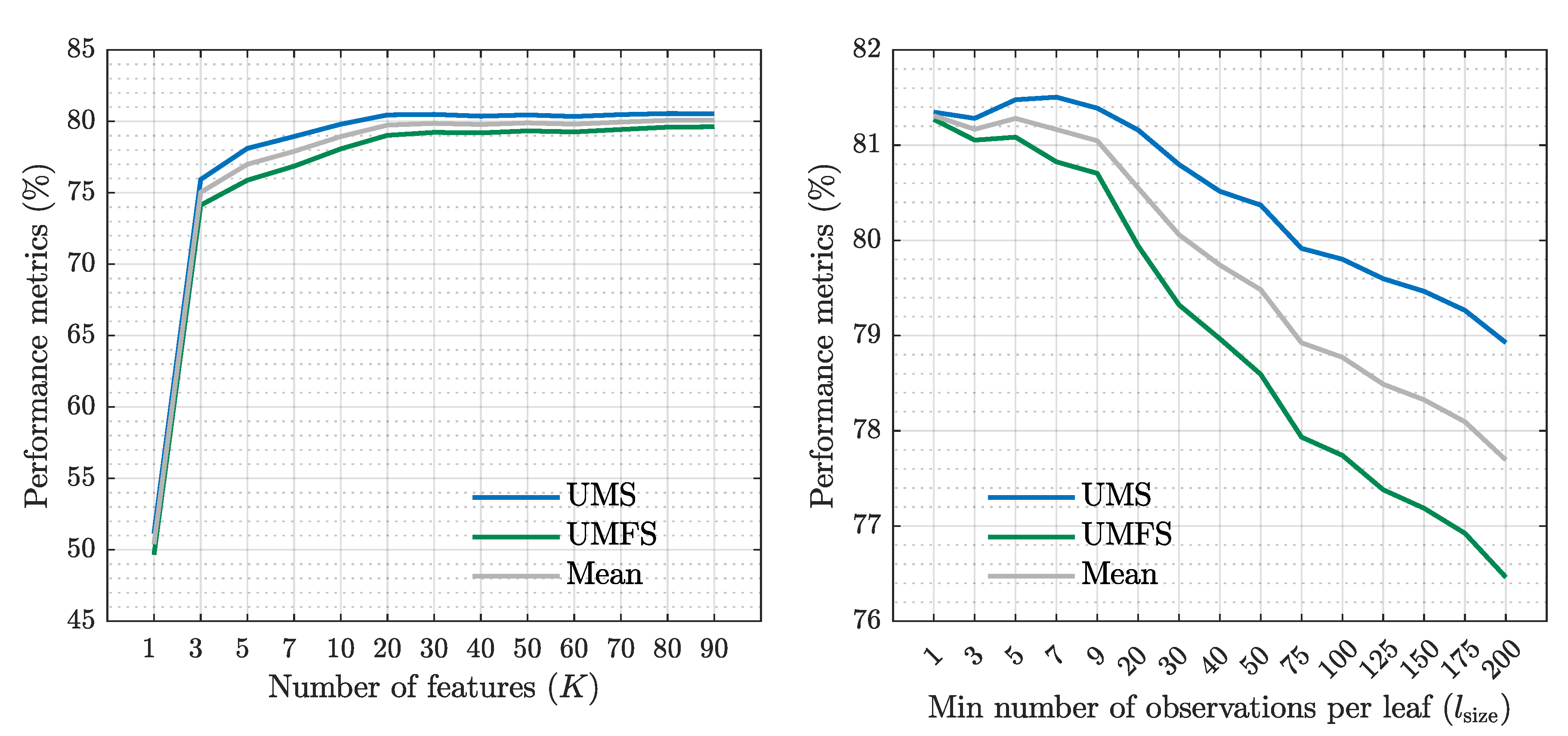
3.3. Classical Machine Learning Architecture

The classical ML algorithm is based on a state-of-the-art solution originally designed for multiclass OHCA rhythm classification during manual CPR [31]. In essence, the algorithm integrates a multiresolution ECG analysis approach, employing the Stationary Wavelet Transform (SWT) for feature extraction and a RF classifier for the subsequent classification. The SWT decomposes the 12 s window into 7 detail coefficients (d1-d7) sub-bands using a Daubechies 4 mother wavelet. A denoised version of the ECG is also reconstructed using the detail coefficients d3 to d7, corresponding to an analysis frequency band of 0.98–31.25 Hz .
From the denoised ECG and the detail coefficients d3-d7, ninety-three features were extracted to characterize OHCA rhythm subtypes, representing over 25 years of research in the field. These features were divided into five analysis domains. Time domain features included characteristics like the mean and the standard deviation of the heart rate [25]; spectral features included classical measures like VF leakage [44] or the power proportion concentrated around the VF-fibrillation band [29]; complexity analysis covered entropy measures like sample or Shannon entropy [45]; statistical analysis measures involved amplitude distribution characteristics; finally, phase space features utilized time-delay embedding to extract dynamics in the ECG. The detailed description of each of the 93 features can be found in [31].
The training set was divided using a 10-fold CV approach to select the best subset of K features and to optimize RF hyperparameters. First, the optimal set of features was selected for each of the 10 training folds that constitute the 10-fold CV. Feature selection was based on a recursive feature elimination (RFE) approach, using the out-of-bag permutation importance as a ranking criterion [46,47]. Permutation importance is an inherent characteristic of the RF classifier that evaluates the significance of each feature by randomly shuffling its values in the training data of each tree in the forest and then measuring the resulting change in the out-of-bag error. In each iteration of the RFE algorithm, features were ranked, and the least important 3% were removed. This process was repeated until the optimal sets of K features, with K = 1 , 3 , 5 , 7 , 10 · j and j = 1 , . . . , 9 , were selected for classification. Once the best K-feature subsets were selected in each of the 10 CV training folds, the RF classifier was optimized. Only one parameter of the RF classifier was considered for optimization: the minimum number of observations per leaf, l size , which controls the depth of the trees and was identified in [31] as essential for preventing overfitting. For every CV training fold and subset of K features, different l size values were trained in the range 1 l size 200 , and evaluated in the corresponding testing fold. The number of trees was set to B = 500 and the number of predictors per split was fixed to the default value K for both feature selection and l size optimization. B = 500 is sufficient to stabilize accuracy without causing overfitting [48] and the default value of the number of predictors per split achieved by far the best performance in [31]. Finally, l size was fixed to the default value l size = 1 during the feature selection process.

3.4. Algorithm Based on CNNs

Figure 3 a) shows in blue the architecture of the multiclass OHCA rhythm classification algorithm based on CNNs. This architecture is based on the one proposed in [30] to discern Sh and NSh rhythms during manual CPR. The filtered ECG (1-D signal of N = 3000 samples), is introduced to a CNN composed of B convolutional blocks (Figure 3 shows a 3-block as an example, B will be a trainable parameter) that extract the high level features of the signal, followed by two fully connected layers for the three-class classification. The b-th convolutional block is comprised of a one-dimensional convolutional layer (Conv1D) with J b filters of width I b , followed by a batch normalization (BN) layer, a rectified linear unit (ReLU), a max-pooling layer and a dropout layer.
The input to the first convolutional block is defined as s 0 ( n , 1 ) = s ^ ecg ( n ) . The expression s b 1 ( n , m ) will refer to the input of block b, or equivalently, the output of block b 1 , where n and m represent the time and filter index, respectively. The output of the Conv1D at b-th convolutional block can be formulated as:
c b ( n , m ) = b m + ρ = 1 J b 1 i = 1 I b w ρ , i m s b 1 ( n + i 1 , ρ )
where the filter weights w ρ , i m , and the biases for channel shifting b m are the learnable parameters adjusted during training.
BN layers modify the output of the preceding layer to prevent complex weight interactions from altering the data distribution. This accelerates training by allowing the use of larger learning rates and improves generalization while reducing overfitting [49]. For every training mini-batch B , a BN layer calculates the channel-wise means μ B , m and variances σ B , m 2 and then normalizes each channel following
c ^ b ( n , m ) = c b ( n , m ) μ B , m σ B , m 2 + ϵ ,
where ϵ is a small value included to ensure numerical stability. The normalized channels are then adjusted through scaling and shifting to optimize the final ReLu layer. As a result, the outputs, z b ( n , m ) , can be expressed as
z b ( n , m ) = γ m · c ^ b ( n , m ) + β m ,
where γ m and β m are trainable parameters. On inference, a moving average of the mini-batch means μ B , m and variances σ B , m 2 observed during training is typically applied in (9).
Max-pooling layers downsample input data by taking the maximum value from each block of K elements along the time dimension n, so that the output for block b can be represented as:
s b ( n , m ) = max z b ( k , m ) k = ( n 1 ) · K + 1 , . . . , n · K
Finally, the ReLU layers add nonlinearity to the network through the activation function f ( x ) = max 0 , x , enabling the model to learn intricate nonlinear mappings.
Zero-padding was applied before the convolution operations, so the only reduction of dimensionality was due to the max-pooling layers ( K = 3 ). The dropout layer at the end of each block serves as a regularization mechanism, operating exclusively during training to prevent overfitting. This layer temporarily disables a randomly chosen fraction of the network’s adjustable parameters. The output of the last convolutional block was flattened and fed to a dense network composed of two fully connected layers with 10 and 3 neurons, respectively. Finally, a softmax layer transformed the output of the final 3 neurons into values ranging from 0 , 1 , representing the probabilities that a given segment corresponds to a Sh ( p Sh ), AS ( p AS ) or OR ( p OR ) rhythm.
The CNN parameters adjusted during the training phase were the following: the number of convolutional blocks B = 3 , 4 , 5 , 6 , the width of the filters I = 2 , 4 , 8 , 16 , 32 , 64 , 92 (the same filter width is considered along the B blocks) and the number of filters which varies from block to block L = J 1 , J 2 , . . . , J B . Six filter configurations, with increasing number of filters (from sparse to dense), were studied: L 1 = ( 1 , 2 , 4 , 8 , 16 , 32 ) , L 2 = ( 2 , 4 , 8 , 16 , 32 , 64 ) , L 3 = ( 4 , 8 , 16 , 32 , 64 , 128 ) , L 4 = ( 6 , 12 , 24 , 48 , 96 , 192 ) , L 5 = ( 8 , 16 , 32 , 64 , 128 , 256 ) , L 6 = ( 10 , 20 , 40 , 80 , 160 , 320 ) . The values in parentheses correspond to the number of filters J b for blocks b = 1 , . . . , 6 . For architecures with B < 6 blocks, central values (with upwards bias) were selected, so for 3, 4 and 5 blocks the L 2 configuration would be for instance: (8,16,32), (4,8,16,32) and (4,8,16,32,64), respectively.

3.5. Algorithm Based on ResNets

The third architecture explored was a ResNet, which mitigates the issue of performance deterioration as layers are added, enabling deeper networks [50]. The main components of a ResNet are residual blocks, which comprise a main path, including convolutional, batch normalization and other typical CNN layers, and a shortcut path, which directly connects the input and the main path output. Be x the input to a residual block, and H ( x ) the desired data transformation; instead of learning this transformation directly, residual blocks focus on learning the difference between the input and the output, called the residual F ( x ) = H ( x ) x . This is achieved by simple addition of the main path and shortcut path outputs, and makes it easier for the network to learn by focusing on refining the input rather than completely transforming it.
Figure 3 b) shows the layout of the ResNet architecture [50] which, similarly to in Jaureguibeitia et al. [23], intended to replicate that of the CNN, deepening the network while maintaining a coherent structure. Similarly to the CNN, the network was composed of B = 3 , 4 , 5 , 6 blocks, each consisting of two residual blocks following the main path pre-activation configuration (conv-BN-ReLu-conv-BN) proposed by Han et al. [51]; the first block of the network was an exception to this rule, and consisted of a single, much simpler conv-BN-ReLU configuration with no shortcut path. Pooling layers were replaced by strided convolutions, which skip every other step in the filtering process. When adjustments to length and depth were needed, the shortcut path of the first residual block included a strided convolution to create a linear projection of the input. As in the CNN, each convolutional layer in the network used an identical filter size selected from I = 2 , 4 , 8 , 16 , 32 , 64 , 92 . Similarly, the possible configurations of number of filters were selected from L 1 L 6 , with the number of filters per block applied to each convolutional layer within that block. Finally, the hidden fully connected layer was replaced by a global average pooling layer, which outputs the mean value of each input channel [52]. The final values of B, I, and configuration L , were all optimized during the training phase.
Both in the CNN and ResNet architectures, the weights and biases of every layer were optimized as to minimize categorical crossentropy, using stochastic gradient descent with a momentum of 0.8. The initial learning rate was fixed at 0.02 and it was reduced by a factor of 0.8 at every epoch. The training process was conducted for 20 epochs, with a batch size of 256 samples [53].

4. Results

Figures 4 and 5 show the results obtained by the classical ML algorithm on the training data. The left panel of Figure 4 shows the mean performance metrics (UMS, UMFS, and average between UMS and UMFS) as a function of the number of features K; these were calculated as the average, across all l size ( i ) values considered, of the CV performance metrics obtained for K-feature and l size = l size ( i ) RF models. The best compromise between model simplicity and performance was obtained for K = 20 as metrics barely increase for a greater value of K. The right panel of Figure 4 shows the CV performance metrics as a function of l size ; RF models of K = 20 features were considered, based on the previous results. In terms of average between UMS and UMFS, the optimal range for l size was 1 < = l size < = 9 , with a significant decline in performance observed for larger values of l size . The value l size = 1 was chosen as optimal, as it produced the most balanced UMS and UMFS results. Figure 5 shows the 30 ECG features with higher probability of selection for the K = 20 and l size = 1 CV RF models. These probabilities were estimated by counting the number of times the features were selected in the 10 iterations of the feature selection algorithm in the 10-fold CV loop. The most important 9 parameters, i.e. those that were selected in the 100% of iterations, were highly heterogeneous, deriving from all detail coefficients as well as from the denoised ECG, and corresponding to complexity (SampEn), time (bCP), statistical (IQR, StdAbs1, Hmb, Hcmp) and phase space domains (SkewPSD). The acronyms used in Figure 5 are the same as those found in [31], where a detailed description of each parameter is provided. Given these results, a single optimal RF configuration was defined, using l size = 1 and the most important K = 20 features as per Figure 5. On a 10-fold CV loop over training data, this configuration obtained identical UMS and UMFS scores of 81.3%. As a single model trained on the complete training data set and evaluated on the test set, it obtained a UMS and UMFS of 85.3% ad 85.1%, respectively (all the details can be cound in Table 1).
The impact of altering the main parameters of the CNN architecture is depicted in Figure 6. The top row shows the CV performance metrics (UMS, UMFS, and average between UMS and UMFS) for a varying filter size I and a fixed filter configuration L 3 . The best performance in terms of average between UMFS and UMS (third column on both rows) was obtained for a filter width of I = 64 , 32 , 32 and 16 when B = 3 , 4 , 5 and B = 6 were used. The bottom row studies the effect of changing the filter configuration when the filter size is fixed at/to these optimal values. The L 3 configuration for B = 5 blocks and the L 5 configuration with B = 6 blocks achieved the best and very similar performances, with the 6-block one being slightly better. Therefore, the optimal model for the CNN architecture was composed of 6 convolutional blocks with 8, 16, 32, 64, 128 and 256 filters, all of them of width 16. In the training set, this model achieved a UMFS and UMS of 83.0% and 84.8%, respectively. In the testing set, the model obtained a UMFS and UMS of 86.1% and 87.5%, respectively (all the details can be found in Table 1).
Figure 7 analyzes the effect of changing the parameters of the ResNet architecture. Similar to CNNs, the filter width was optimized first with the filter configuration fixed at L 3 (first row) for fixed optimal filter sizes and then followed by the selection of filter configuration (second row). The best classification results were obtained for 4 blocks. Adding a fifth block increased the complexity of the network (number of trainable parameters) and slightly decreased performance. Using only 3 blocks resulted in a large decrease in performance, or an overly simplistic model. As the third column of the first row shows, the best performance in terms of average between UMFS and UMS was obtained for I = 32 when B 5 and I = 16 when B = 6 . With the filter width fixed, the second row of Figure 7 shows that the best performance was achieved for 4 blocks and L 4 filter configuration. Thus, the optimal configuration of the ResNet architecture consisted of 4 blocks containing 6, 12, 24 and 48 filters respectively, all of them of width 32. That is, the ResNet input block used 6 filters and the remaining 3 blocks used 12, 24 and 48 filters in each of the residual blocks. In the training set, this configuration obtained a UMFS and UMS of 86.9% and 86.6%, respectively. In the testing set, the ResNet model obtained a value of 88.3% for both the UMFS and the UMS (all the details can be found in Table 1).
Table I shows the results of the OHCA rhythm classification algorithms based on classical ML, CNN and ResNet models when the aforementioned optimal configurations were applied in to the testing set. As the summarizing metrics demonstrate, the DL-based algorithms performed better than the traditional ML ones. The CNN model outperformed the RF model by 1 percentage point in UMFS and 2 percentage points in UMS and ACC. The ResNet was the best-performing model, outperforming the CNN model by approximately 2 percentage points in UMFS and ACC and one percentage point in UMS.
Given the importance of the Sh/NSh discrimination during resuscitation therapy and as additional experiment, the best performing method (ResNet) was adapted for the binary Sh/NSh classification task. For this experiment, AS and OR rhythms were grouped into the NSh category, using 9666 segments (1252 Sh, 8414 NSh) to train and 5813 segments (1154 Sh, 4659 NSh) to test the model. The optimal ResNet architecture for this problem was selected in an analogous manner to that for the 3-class problem. Performance was evaluated in terms of sensitivity (SE, the proportion of correctly classified Sh rhythms) and specificity (SP, the proportion of correctly classified NSh rhythms), in line with the minimum performance requirements for Sh/Nsh discrimination recommended by the AHA; the balanced accuracy (the mean of SE and SP) was chosen as summarizing metric. Figure 8 shows the performance metrics obtained across the 10-fold CV loop in the training set. As in previous figures, the top row analyzes the impact of altering the width of the filters, I, while the bottom one explores the impact of altering the configuration of the filters, L , for a fixed filter size. As shown in the third panel of the bottom row, the L 6 configuration with 3 and 4 blocks and I = 32 achieved the maximum BAC, with the 4-block one being slightly higher. This architecture obtained a SE/SP/BAC scores of 85.5%/98.6%/92.0% and 90.6%/98.5%/94.6% in the training and testing sets, respectively.

5. Discussion

The adoption of mechanical CPR devices has significantly increased in recent years, primarily through two main technologies: LDB and piston-driven mechanical CC devices. Mechanical CPR guarantees high-quality CCs when manual CPR is i) subjected to fatigue, ii) practically challenging or iii) cannot be delivered safely.
This is, to the best of our knowledge, the first study that covers multiclass OHCA rhythm classification during mechanical CPR. The proposed architectures integrated the collective knowledge derived from active research in the rhythm classification field, considering an adaptive filter for CPR artifact suppression, followed by a multiclass rhythm classifier for which the performance of a traditional ML algorithm and two DL architectures based on CNNs and ResNets were compared.
DL-based algorithms outperformed the classical ML algorithm by at least 2 percentage points in UMS and ACC. Considering that the classical ML algorithm relies on over 20 years of expert knowledge in ECG feature engineering for OHCA rhythm classification, these results highlight the power of DL algorithms to learn discriminative features by leveraging all the hidden information in the ECG. This simplifies the feature extraction process, saving time and, more importantly, improving the quality of the features extracted.
The algorithm based on ResNets offered the best performance, achieving a UMFS, UMS and ACC of 88.3%, 88.3% and 88.2% for the 3-class classification task, respectively. This performance is similar to that obtained in [31], the only study in the literature that analyzes multiclass OHCA rhythm classification during manual CPR. The characteristics of manual compressions are rescuer dependant, which means the variability of the resulting artifacts anticipates a more complex filtering challenge. However, manual artifacts showed significantly smaller artifact amplitudes and less harmonic components (smaller bandwidths) compared to LDB artifacts, and this balance resulted in similar levels of accuracy [40,54,55]. For the Sh/NSh problem, the BAC was 94.6%, with a SE of 90.6% and a SP of 98.5%. This is a very important problem since it addresses shock advice decisions during CPR. Shock advice algorithms for defibrillators are normally tested on artifact-free data. In that scenario, the AHA requires a minimum SE and SP of 90% and 95%, respectively[56]. Our solution met those requirements.
The database used in this study was fully derived from OHCA cases. It is unclear whether the proposed algorithms would perform differently for in-hospital data; however, given that in-hospital resuscitation does not entail differences in LDB-CPR, it is tempting to argue that the analysis and results we have presented for OHCA patients also will be valid for in hospital cardiac arrest and CPR.
In conclusion, this study presents the first method for an automatic and clinically safe multiclass OHCA rhythm analysis during LBD-CPR. The proposed solution together with already available solutions for piston-driven [38] and manual CCs [31] would cover rhythm analysis in every CPR scenario. This may open the possibility of a reliable multiclass OHCA rhythm analysis during CPR, contributing to guide therapy while reducing no-flow intervals, and thereby improving survival in OHCA. In addition, this method could be used to automatically annotate large OHCA datasets in order to retrospectively analyze the effects of therapy on OHCA outcome, contributing to identify those treatments that increase OHCA survival.

Acknowledgments

This research has been partially supported by the MCIN/ AEI/10.13039/501100011033/ and by FEDER Una manera de hacer Europa through grant PID2021-122727OB-I00. Additional support has been provided by the Basque Government through grant IT1717-22.

References

  1. Gräsner, J.T.; Herlitz, J.; Tjelmeland, I.B.; Wnent, J.; Masterson, S.; Lilja, G.; Bein, B.; Böttiger, B.W.; Rosell-Ortiz, F.; Nolan, J.P.; et al. European Resuscitation Council Guidelines 2021: epidemiology of cardiac arrest in Europe. Resuscitation 2021, 161, 61–79. [Google Scholar] [PubMed]
  2. Soar, J.; Böttiger, B.W.; Carli, P.; Couper, K.; Deakin, C.D.; Djärv, T.; Lott, C.; Olasveengen, T.; Paal, P.; Pellis, T.; et al. European resuscitation council guidelines 2021: adult advanced life support. Resuscitation 2021, 161, 115–151. [Google Scholar] [PubMed]
  3. Olasveengen, T.M.; Semeraro, F.; Ristagno, G.; Castren, M.; Handley, A.; Kuzovlev, A.; Monsieurs, K.G.; Raffay, V.; Smyth, M.; Soar, J.; et al. European resuscitation council guidelines 2021: basic life support. Resuscitation 2021, 161, 98–114. [Google Scholar] [PubMed]
  4. Gough, C.J.; Nolan, J.P. The role of adrenaline in cardiopulmonary resuscitation. Critical Care 2018, 22, 1–8. [Google Scholar]
  5. Kvaløy, J.T.; Skogvoll, E.; Eftestøl, T.; Gundersen, K.; Kramer-Johansen, J.; Olasveengen, T.M.; Steen, P.A. Which factors influence spontaneous state transitions during resuscitation? Resuscitation 2009, 80, 863–869. [Google Scholar]
  6. Nordseth, T.; Bergum, D.; Edelson, D.P.; Olasveengen, T.M.; Eftestøl, T.; Wiseth, R.; Abella, B.S.; Skogvoll, E. Clinical state transitions during advanced life support (ALS) in in-hospital cardiac arrest. Resuscitation 2013, 84, 1238–1244. [Google Scholar]
  7. Nordseth, T.; Niles, D.E.; Eftestøl, T.; Sutton, R.M.; Irusta, U.; Abella, B.S.; Berg, R.A.; Nadkarni, V.M.; Skogvoll, E. Rhythm characteristics and patterns of change during cardiopulmonary resuscitation for in-hospital paediatric cardiac arrest. Resuscitation 2019, 135, 45–50. [Google Scholar]
  8. Thakor, N.V.; Zhu, Y.S.; Pan, K.Y. Ventricular tachycardia and fibrillation detection by a sequential hypothesis testing algorithm. IEEE Transactions on Biomedical Engineering 1990, 37, 837–843. [Google Scholar]
  9. Jekova, I.; Krasteva, V. Real time detection of ventricular fibrillation and tachycardia. Physiological measurement 2004, 25, 1167. [Google Scholar]
  10. Irusta, U.; Ruiz, J. An algorithm to discriminate supraventricular from ventricular tachycardia in automated external defibrillators valid for adult and paediatric patients. Resuscitation 2009, 80, 1229–1233. [Google Scholar]
  11. Neurauter, A.; Eftestøl, T.; Kramer-Johansen, J.; Abella, B.S.; Sunde, K.; Wenzel, V.; Lindner, K.H.; Eilevstjønn, J.; Myklebust, H.; Steen, P.A.; et al. Prediction of countershock success using single features from multiple ventricular fibrillation frequency bands and feature combinations using neural networks. Resuscitation 2007, 73, 253–263. [Google Scholar] [PubMed]
  12. Kwok, H.; Coult, J.; Drton, M.; Rea, T.D.; Sherman, L. Adaptive rhythm sequencing: A method for dynamic rhythm classification during CPR. Resuscitation 2015, 91, 26–31. [Google Scholar] [PubMed]
  13. Chicote, B.; Irusta, U.; Alcaraz, R.; Rieta, J.J.; Aramendi, E.; Isasi, I.; Alonso, D.; Ibarguren, K. Application of entropy-based features to predict defibrillation outcome in cardiac arrest. Entropy 2016, 18, 313. [Google Scholar] [CrossRef]
  14. Chicote, B.; Irusta, U.; Aramendi, E.; Alcaraz, R.; Rieta, J.J.; Isasi, I.; Alonso, D.; Baqueriza, M.d.M.; Ibarguren, K. Fuzzy and sample entropies as predictors of patient survival using short ventricular fibrillation recordings during out of hospital cardiac arrest. Entropy 2018, 20, 591. [Google Scholar] [CrossRef]
  15. Cabello, D.; Barro, S.; Salceda, J.; Ruiz, R.; Mira, J. Fuzzy K-nearest neighbor classifiers for ventricular arrhythmia detection. International journal of bio-medical computing 1991, 27, 77–93. [Google Scholar]
  16. Rad, A.B.; Eftestøl, T.; Engan, K.; Irusta, U.; Kvaløy, J.T.; Kramer-Johansen, J.; Wik, L.; Katsaggelos, A.K. ECG-based classification of resuscitation cardiac rhythms for retrospective data analysis. IEEE transactions on biomedical engineering 2017, 64, 2411–2418. [Google Scholar]
  17. Cheng, P.; Dong, X. Life-threatening ventricular arrhythmia detection with personalized features. IEEE access 2017, 5, 14195–14203. [Google Scholar]
  18. Li, Q.; Rajagopalan, C.; Clifford, G.D. Ventricular fibrillation and tachycardia classification using a machine learning approach. IEEE Transactions on Biomedical Engineering 2013, 61, 1607–1613. [Google Scholar]
  19. Rad, A.B.; Eftestøl, T.; Irusta, U.; Kvaløy, J.T.; Wik, L.; Kramer-Johansen, J.; Katsaggelos, A.K.; Engan, K. An automatic system for the comprehensive retrospective analysis of cardiac rhythms in resuscitation episodes. Resuscitation 2018, 122, 6–12. [Google Scholar]
  20. Figuera, C.; Irusta, U.; Morgado, E.; Aramendi, E.; Ayala, U.; Wik, L.; Kramer-Johansen, J.; Eftestøl, T.; Alonso-Atienza, F. Machine learning techniques for the detection of shockable rhythms in automated external defibrillators. PloS one 2016, 11, e0159654. [Google Scholar]
  21. Picon, A.; Irusta, U.; Álvarez-Gila, A.; Aramendi, E.; Alonso-Atienza, F.; Figuera, C.; Ayala, U.; Garrote, E.; Wik, L.; Kramer-Johansen, J.; et al. Mixed convolutional and long short-term memory network for the detection of lethal ventricular arrhythmia. PloS one 2019, 14, e0216756. [Google Scholar]
  22. Hajeb-M, S.; Cascella, A.; Valentine, M.; Chon, K. Deep neural network approach for continuous ECG-based automated external defibrillator shock advisory system during cardiopulmonary resuscitation. Journal of the American Heart Association 2021, 10, e019065. [Google Scholar] [PubMed]
  23. Jaureguibeitia, X.; Zubia, G.; Irusta, U.; Aramendi, E.; Chicote, B.; Alonso, D.; Larrea, A.; Corcuera, C. Shock decision algorithms for automated external defibrillators based on convolutional networks. IEEE Access 2020, 8, 154746–154758. [Google Scholar]
  24. Alonso, E.; Aramendi, E.; Daya, M.; Irusta, U.; Chicote, B.; Russell, J.K.; Tereshchenko, L.G. Circulation detection using the electrocardiogram and the thoracic impedance acquired by defibrillation pads. Resuscitation 2016, 99, 56–62. [Google Scholar]
  25. Elola, A.; Aramendi, E.; Irusta, U.; Del Ser, J.; Alonso, E.; Daya, M. ECG-based pulse detection during cardiac arrest using random forest classifier. Medical & biological engineering & computing 2019, 57, 453–462. [Google Scholar]
  26. Alwan, Y.; Cvetković, Z.; Curtis, M.J. Methods for improved discrimination between ventricular fibrillation and tachycardia. IEEE Transactions on Biomedical Engineering 2017, 65, 2143–2151. [Google Scholar]
  27. Cheskes, S.; Schmicker, R.H.; Christenson, J.; Salcido, D.D.; Rea, T.; Powell, J.; Edelson, D.P.; Sell, R.; May, S.; Menegazzi, J.J.; et al. Perishock pause: an independent predictor of survival from out-of-hospital shockable cardiac arrest. Circulation 2011, 124, 58–66. [Google Scholar]
  28. Ruiz de Gauna, S.; Irusta, U.; Ruiz, J.; Ayala, U.; Aramendi, E.; Eftestøl, T. Rhythm analysis during cardiopulmonary resuscitation: past, present, and future. BioMed research international 2014, 2014, 386010. [Google Scholar]
  29. Ayala, U.; Irusta, U.; Ruiz, J.; Eftestøl, T.; Kramer-Johansen, J.; Alonso-Atienza, F.; Alonso, E.; González-Otero, D. A reliable method for rhythm analysis during cardiopulmonary resuscitation. BioMed research international 2014, 2014, 872470. [Google Scholar]
  30. Isasi, I.; Irusta, U.; Aramendi, E.; Eftestøl, T.; Kramer-Johansen, J.; Wik, L. Rhythm analysis during cardiopulmonary resuscitation using convolutional neural networks. Entropy 2020, 22, 595. [Google Scholar] [CrossRef]
  31. Isasi, I.; Irusta, U.; Rad, A.B.; Aramendi, E.; Zabihi, M.; Eftestøl, T.; Kramer-Johansen, J.; Wik, L. Automatic cardiac rhythm classification with concurrent manual chest compressions. IEEE Access 2019, 7, 115147–115159. [Google Scholar]
  32. Wik, L.; Olsen, J.A.; Persse, D.; Sterz, F.; Lozano Jr, M.; Brouwer, M.A.; Westfall, M.; Souders, C.M.; Malzer, R.; van Grunsven, P.M.; Manual, vs.; et al. integrated automatic load-distributing band CPR with equal survival after out of hospital cardiac arrest. The randomized CIRC trial. Resuscitation 2014, 85, 741–748. [Google Scholar] [PubMed]
  33. Rubertsson, S.; Lindgren, E.; Smekal, D.; Östlund, O.; Silfverstolpe, J.; Lichtveld, R.A.; Boomars, R.; Ahlstedt, B.; Skoog, G.; Kastberg, R.; et al. Mechanical chest compressions and simultaneous defibrillation vs conventional cardiopulmonary resuscitation in out-of-hospital cardiac arrest: the LINC randomized trial. Jama 2014, 311, 53–61. [Google Scholar] [PubMed]
  34. Krep, H.; Mamier, M.; Breil, M.; Heister, U.; Fischer, M.; Hoeft, A. Out-of-hospital cardiopulmonary resuscitation with the AutoPulse™ system: A prospective observational study with a new load-distributing band chest compression device. Resuscitation 2007, 73, 86–95. [Google Scholar]
  35. Ong, M.E.H.; Mackey, K.E.; Zhang, Z.C.; Tanaka, H.; Ma, M.H.M.; Swor, R.; Shin, S.D. Mechanical CPR devices compared to manual CPR during out-of-hospital cardiac arrest and ambulance transport: a systematic review. Scandinavian journal of trauma, resuscitation and emergency medicine 2012, 20, 1–10. [Google Scholar]
  36. Putzer, G.; Braun, P.; Zimmermann, A.; Pedross, F.; Strapazzon, G.; Brugger, H.; Paal, P. LUCAS compared to manual cardiopulmonary resuscitation is more effective during helicopter rescue—a prospective, randomized, cross-over manikin study. The American journal of emergency medicine 2013, 31, 384–389. [Google Scholar]
  37. Ashton, A.; McCluskey, A.; Gwinnutt, C.; Keenan, A. Effect of rescuer fatigue on performance of continuous external chest compressions over 3 min. Resuscitation 2002, 55, 151–155. [Google Scholar]
  38. Isasi, I.; Irusta, U.; Elola, A.; Aramendi, E.; Ayala, U.; Alonso, E.; Kramer-Johansen, J.; Eftestøl, T. A machine learning shock decision algorithm for use during piston-driven chest compressions. IEEE transactions on biomedical engineering 2018, 66, 1752–1760. [Google Scholar]
  39. Isasi, I.; Irusta, U.; Aramendi, E.; Olsen, J.; Wik, L. Shock decision algorithm for use during load distributing band cardiopulmonary resuscitation. Resuscitation 2021, 165, 93–100. [Google Scholar]
  40. Isasi, I.; Irusta, U.; Aramendi, E.; Ayala, U.; Alonso, E.; Kramer-Johansen, J.; Eftestøl, T. A multistage algorithm for ECG rhythm analysis during piston-driven mechanical chest compressions. IEEE Transactions on Biomedical Engineering 2018, 66, 263–272. [Google Scholar]
  41. Lerner, E.B.; Persse, D.; Souders, C.M.; Sterz, F.; Malzer, R.; Lozano Jr, M.; Westfall, M.; Brouwer, M.A.; van Grunsven, P.M.; Whitehead, A.; et al. Design of the Circulation Improving Resuscitation Care (CIRC) Trial: a new state of the art design for out-of-hospital cardiac arrest research. Resuscitation 2011, 82, 294–299. [Google Scholar] [CrossRef] [PubMed]
  42. Xiao, Y.; Ma, L.; Ward, R.K. Fast RLS Fourier analyzers capable of accommodating frequency mismatch. Signal Processing 2007, 87, 2197–2212. [Google Scholar] [CrossRef]
  43. Irusta, U.; Ruiz, J.; de Gauna, S.R.; Eftestl, T.; Kramer-Johansen, J. A least mean-square filter for the estimation of the cardiopulmonary resuscitation artifact based on the frequency of the compressions. IEEE Transactions on Biomedical Engineering 2009, 56, 1052–1062. [Google Scholar] [PubMed]
  44. Kuo, S. Computer detection of ventricular fibrillation. Proc. of Computers in Cardiology, IEEE Comupter Society.
  45. Alonso-Atienza, F.; Morgado, E.; Fernandez-Martinez, L.; Garcia-Alberola, A.; Rojo-Alvarez, J.L. Detection of life-threatening arrhythmias using feature selection and support vector machines. IEEE Transactions on Biomedical Engineering 2013, 61, 832–840. [Google Scholar]
  46. Pang, H.; George, S.L.; Hui, K.; Tong, T. Gene selection using iterative feature elimination random forests for survival outcomes. IEEE/ACM Transactions on Computational Biology and Bioinformatics 2012, 9, 1422–1431. [Google Scholar]
  47. Shen, K.Q.; Ong, C.J.; Li, X.P.; Hui, Z.; Wilder-Smith, E.P. A feature selection method for multilevel mental fatigue EEG classification. IEEE transactions on biomedical engineering 2007, 54, 1231–1237. [Google Scholar]
  48. Breiman, L. Random forests Mach Learn 45 (1): 5–32, 2001.
  49. Ioffe, S. Batch normalization: Accelerating deep network training by reducing internal covariate shift. arXiv preprint arXiv:1502.03167, arXiv:1502.03167 2015.
  50. He, K.; Zhang, X.; Ren, S.; Sun, J. Deep residual learning for image recognition. In Proceedings of the Proceedings of the IEEE conference on computer vision and pattern recognition, 2016, pp.
  51. Han, D.; Kim, J.; Kim, J. Deep pyramidal residual networks. In Proceedings of the Proceedings of the IEEE conference on computer vision and pattern recognition, 2017, pp.
  52. Lin, M.; Chen, Q.; Yan, S. Network in network. arXiv preprint arXiv:1312.4400, arXiv:1312.4400 2013.
  53. Sutskever, I.; Martens, J.; Dahl, G.; Hinton, G. On the importance of initialization and momentum in deep learning. In Proceedings of the International conference on machine learning. PMLR; 2013; pp. 1139–1147. [Google Scholar]
  54. Isasi, I.; Irusta, U.; Aramendi, E.; Age, J.; Wik, L. Characterization of the ECG compression artefact caused by the AutoPulse device. Resuscitation 2017, 118, e38. [Google Scholar]
  55. Isasi, I.; Irusta, U.; Aramendi, E.; Ayala, U.; Alonso, E.; Kramer-Johansen, J.; Eftest, T.; et al. Removing piston-driven mechanical chest compression artefacts from the ECG. In Proceedings of the 2017 Computing in Cardiology (CinC). IEEE; 2017; pp. 1–4. [Google Scholar]
  56. Kerber, R.E.; Becker, L.B.; Bourland, J.D.; Cummins, R.O.; Hallstrom, A.P.; Michos, M.B.; Nichol, G.; Ornato, J.P.; Thies, W.H.; White, R.D.; et al. Automatic external defibrillators for public access defibrillation: recommendations for specifying and reporting arrhythmia analysis algorithm performance, incorporating new waveforms, and enhancing safety: a statement for health professionals from the American Heart Association Task Force on Automatic External Defibrillation, Subcommittee on AED Safety and Efficacy. Circulation 1997, 95, 1677–1682. [Google Scholar]
Figure 1. A 70 s interval from an OHCA episode. From top to bottom: a) ECG, b) instantaneous CC rate, c) thoracic impedance (TI) and d) filtered ECG (filtered only in the interval corresponding to mechanical CCs in the database segment). CC instants are depicted as blue circles in TI signal. Activity shows manual CPR (first 15 s ), followed by a pause for the LDB device application, and resumption of mechanical CPR (last 20 s ). The interval highlighted in green in panel a) corresponds to a 22 s segment included in the study dataset. The first 6 s (light green), free of CC artifacts, were used to annotate the ground truth rhythm (organized) of the patient, while the last 16 s with artifact (dark green) were used to develop the algorithms.
Preprints 151431 g001
Figure 2. Panel a) illustrates the adaptive RLS filtering schema, while panel b) shows the input and output signals in the interval correponding to the last 16 s of the database segment highligted in dark green in Figure 1. From top to bottom: the corrupted ECG, s cor ( n ) , the estimated CC artifact, s ^ cc ( n ) and the filtered ECG, s ^ ecg ( n ) . The highlighted segment corresponds to the 12 s interval used for the development of the classification algorithms, thus avoiding filtering transients.
Preprints 151431 g002
Figure 3. Architecture of a) CNN-based and b) RestNet-based rhythm classifiers.
Preprints 151431 g003
Figure 4. Cross-validation performance metrics (UMFS, UMS and average between UMFS and UMS) for the classic machine learning algorithm as a function of the number of features K (left panel) and the minimum number of observations per leaf l size (right panel). The right panel corresponds to K = 20 .
Preprints 151431 g004
Figure 5. Selection probability for the 30 most selected features by the RF classifier in the 10 iterations of the 10-fold CV loop.
Preprints 151431 g005
Figure 6. Performance of the CNN architecture as a function of the configurable parameters of the network: the number of blocks (B), the filter width (I), and the filter configuration ( L ). The first row shows the effect of the filter width, I, for networks with L 3 configuration. The second row shows the effect of the filter configurations, from dense ( L 6 ) to sparse ( L 1 ), for the optimal I values.
Preprints 151431 g006
Figure 7. Performance of the ResNet architecture as a function of the configurable parameters of the network: the number of blocks (B), the filter width (I), and the filter configuration ( L ). The first row shows the effect of the filter width, I, for networks with L 3 configuration. The second row shows the effect of the filter configurations, from dense ( L 6 ) to sparse ( L 1 ), for the optimal I values.
Preprints 151431 g007
Figure 8. Performance of the ResNet architecture for the binary Sh/NSh classification in terms of the the configurable parameters of the network: the number of blocks (B), the filter width (I), and the filter configuration ( L ). The first row shows the effect of the filter width, I, for networks with L 3 configuration. The second row shows the effect of the filter configurations, from dense ( L 6 ) to sparse ( L 1 ), for the optimal I values.
Preprints 151431 g008
Table 1. Performance metrics obtained by the OHCA multiclass algorithms on the testing set.
SE (%) PPV (%) bad   hbox (%) Sum. metrics
Models AS OR Sh AS OR Sh AS OR Sh UMFS UMS ACC
ML 80.1 85.1 90.7 76.8 87.2 90.7 78.4 86.1 90.7 85.1 85.3 83.8
CNN 84.3 84.1 94.2 78.9 91.2 85.1 81.5 87.5 89.4 86.1 87.5 85.5
ResNet 83.8 89.2 92.0 81.0 90.1 94.1 82.4 89.6 93.0 88.3 88.3 88.2
Disclaimer/Publisher’s Note: The statements, opinions and data contained in all publications are solely those of the individual author(s) and contributor(s) and not of MDPI and/or the editor(s). MDPI and/or the editor(s) disclaim responsibility for any injury to people or property resulting from any ideas, methods, instructions or products referred to in the content.
Copyright: This open access article is published under a Creative Commons CC BY 4.0 license, which permit the free download, distribution, and reuse, provided that the author and preprint are cited in any reuse.
Prerpints.org logo

Preprints.org is a free preprint server supported by MDPI in Basel, Switzerland.

Subscribe

Disclaimer

Terms of Use

Privacy Policy

Privacy Settings

© 2025 MDPI (Basel, Switzerland) unless otherwise stated