
Submitted:
12 November 2024
Posted:
13 November 2024
You are already at the latest version
Abstract
Cardiovascular diseases are the leading cause of death globally, highlighting the need for accurate diagnostic tools. To address this issue, we introduce a novel approach for based arrhythmia detection based on electrocardiogram (ECG) that incorporates explainable artificial intelligence through three key methods. First, we developed an enhanced R peak detection method that integrates domain-specific knowledge into the ECG, improving peak identification accuracy by accounting for the characteristic features of R peaks. Second, we proposed an arrhythmia classification method utilizing a modified convolutional neural network (CNN) architecture with additional convolutional and batch normalization layers. This model processes a triad of cardio cycles–the preceding, current, and following cycles–to capture temporal dependencies and hidden features related to arrhythmias. Third, we implemented an interpretation method that explains CNN’s decisions using clinically relevant features, making the results understandable to clinicians. Using the MIT-BIH database, our approach achieved an accuracy of 99.43%, with F1-scores approaching 100% for major arrhythmia classes. The integration of these methods enhances both the performance and transparency of arrhythmia detection systems.
Keywords:
Electrocardiography (ECG)
; arrhythmia detection
; ECG classification
; ECG interpretation
; explainable artificial intelligence (XAI)
; transparent artificial intelligence
; deep learning
1. Introduction
According to statistics from the World Health Organization, cardiovascular diseases are the leading cause of death worldwide [1,2]. Currently, there are many tools and means available to help clinicians prevent or detect heart problems. One of the most common methods is electrocardiography (ECG). ECG allows for the graphical recording of electrical phenomena from the human body that occurs in the heart muscle during its activity. The curve obtained from recording such activity is called an electrocardiogram or ECG. Thus, an ECG is a recording of fluctuations in the potential difference that occur in the heart during its excitation [3]. A standard ECG recording consists of 12 leads obtained from 10 electrodes [4].
The nature of the ECG is pseudoperiodic. The ECG consists of cardio cycles called QRST complexes (Figure 1). The appearance of the cardio cycle allows clinicians to determine the presence of potential heart pathologies from the ECG. It is important to note that the cardio cycle is visually identified by a clinician based on the R peak of the signal. It is also worth mentioning that existing datasets, in which specific heart pathologies are annotated, are also tied to the cardio cycle. Figure 1 shows the leading indicators (peaks and segments) clinicians use to analyze the cardio cycle for potential pathology.
Since there are currently many possible types of abnormalities in ECG and large volumes of ECG recordings (such as Holter monitoring), the analysis process can be time-consuming and prone to numerous errors. Therefore, information technology methods and approaches are used to address these issues. Due to the rapid development of artificial intelligence (AI) systems, tools like machine learning (ML) and deep learning (DL) have gained widespread use for classifying ECG pathologies.
The use of convolutional neural networks (CNNs) [5], as a DL method [6], for classifying ECGs has already demonstrated significant effectiveness in detecting various heart pathologies, such as arrhythmias, myocarditis, ischemic heart disease, and more [7,8]. Despite the significant advances in this field, the functioning of DL models remains a “black box” for end users [9], which is highly critical in a sensitive field like medicine [10].
Despite numerous existing solutions for ECG classification, several open problems remain unaddressed. In this work, we tackle unresolved issues in ECG analysis using DL that have been neglected or only partially considered. These issues include (i) low accuracy in R peak detection when R peaks exhibit atypical features, (ii) the inability of current classifiers to identify all possible arrhythmias, especially those underrepresented in available datasets due to class imbalance, and (iii) a lack of explainability and transparency in DL model decisions for end users (doctors).
Considering these challenges, the main contributions of this article are as follows:
- A method for identifying R peaks in ECGs: We integrate domain-specific knowledge to enhance R peak detection accuracy, allowing for more precise identification compared to existing methods.
- A method for classifying heart arrhythmias from ECGs: By presenting the input signal as three consecutive cardio cycles and using a modified CNN architecture, we improve classification quality over traditional approaches.
- A method for interpreting DL model classification results: We use features that are understandable to doctors, making the classification decisions transparent and enhancing explainability for end users.
The article’s structure is as follows: Section 2 presents a review of current approaches for detecting heart rhythm, sequence, and contraction force disorders (arrhythmias) from ECGs using explainable AI (XAI) methods. Section 3 describes the proposed approach to solving the problem, which consists of three methods: R peak identification in ECGs, arrhythmia classification in ECGs, and classification result interpretation. Section 4 presents the experimental results of the proposed approach and a discussion.
2. Related Works
Preparing ECG data for use in DL models involves the mandatory segmentation of cardio cycles based on R peaks in the ECG. This approach is driven by the pseudoperiodic nature of ECGs, where the unit of heart activity analysis is the cardio cycle (i.e., QRST complex), and the accuracy of its detection depends on identifying the R peak. At the same time, the precision of R peak identification is crucial, as it affects the effectiveness of applying DL methods to solve the problem of classifying heart arrhythmias.
Currently, there are many approaches to detecting R peaks in ECGs, most of which show an efficiency rate exceeding 99%. However, many studies either indicate a significant margin of error or do not mention it at all when calculating statistical metrics. For example, in studies [11,12], high accuracy in peak detection was achieved, but the allowable error was ±75 ms, creating a total error window of 150 ms, which exceeds the normal duration of the QRST complex.
Since the medical field demands extremely high precision, such errors in studies can be critical. Therefore, researchers like B. Porr and P. W. Macfarlane [13] conducted an analysis of various methods for R peak detection, including Pan and Tompkins by Fariha et al. [14], Hamilton and Tompkins by Ahmad et al. [15], and Christov by Rahul et al. [16]. B. Porr and P. W. Macfarlane established that almost every study reported very high accuracy, above 98%, which can be explained using a large permissible error when calculating the accuracy of the proposed methods. The authors concluded that most experimental studies rely on an error of 100 ms or more, which is too high for real clinical cases involving ECGs. As a result, the task of identifying R peaks with minimal error remains relevant and requires further research.
The next step in ECG analysis, following R peak detection, is the classification of QRST complexes with R peaks according to pathology classes. There are numerous studies on the application of DL models for ECG classification.
For instance, Hassan et al. [17] trained a CNN-BiLSTM to classify five types of heart arrhythmias using the MIT-BIH dataset. They demonstrated that their DL model could classify heart arrhythmias with 98% accuracy, 91% sensitivity, and 91% specificity. Liu et al. [18] proposed an ensemble of LSTM and CNN, which achieved 99.1% accuracy, 99.3% sensitivity, and 98.5% specificity in classifying ECGs. Notably, the authors obtained these results by classifying ECGs into only four classes, excluding the “everything else” class. Xu et al. [19] developed a CNN classifier that categorizes ECGs into five classes, including “normal” and “others.” However, their proposed method only allows the classification of three pathologies, covering a limited set of potential conditions.
In studies by Degirmenci et al. [20] and Rohmantri et al. [21], high classification accuracy was achieved using 2D images of ECGs with a size of 64x64 as input data for classifying arrhythmic heartbeats. There are also several works that transform one-dimensional signals into two-dimensional representations like spectrograms or scalograms, including [22]. Despite achieving high classification accuracy, these approaches result in significant computational costs, making them inefficient for real-time applications and devices with limited computing power. Additionally, the cited works do not utilize an “all other” class, which could potentially worsen classification outcomes.
In their study, Abdelhafid et al. [23] focused on classifying ECG arrhythmias using five classes without the “others” class. This likely contributed to the high classification metrics, but excluding the “others” class may not reflect real clinical cases, as such an approach ignores signals that do not fit predefined categories. Furthermore, their model takes input data for only one cardio cycle. Since the “Premature Ventricular Contraction” (PVC) class is included, this amount of data may be insufficient for classification, as this pathology is characterized by a “compensatory pause,” which requires neighboring cardio cycles for detection. Thus, to effectively and accurately detect heart arrhythmias, it is crucial to develop a DL model that balances accuracy, computational complexity, and the ability to classify a greater number of pathologies, particularly a class that represents all other underrepresented conditions.
Singh and Sharma [24] introduced a deep CNN for arrhythmia interpretation and classification, which demonstrated high accuracy and efficiency. However, like other studies, they faced high computational requirements when using the proposed model in real-world applications. In addition, their study did not address the classification of signals that do not fall into the previous classes, which is crucial for practical applications.
In a recent paper, Ayano et al. [25] suggested an interpretive DL model for 12-lead ECG diagnosis. Their work stands out due to its interpretation and careful analysis of multiplexes, offering a detailed understanding of the diagnostic process. However, the complexity of their model may hinder its use in the absence of significant computing resources, as high interpretation often comes at the cost of computational complexity.
From the analysis above, we see that current approaches do not provide a full interpretation of the classification results that can be transparent and understandable to doctors in practical conditions. Specifically, we point out several issues that warrant further investigation:
- High error rates in R peak identification.
- A limited number of classified pathology classes.
- Classification based on a single cardio cycle without considering preceding or subsequent cycles, thereby ignoring hidden features from adjacent cycles.
- High computational complexity in pathology classification tasks.
- A lack of explainability in DL model decisions using features understandable to healthcare professionals.
Therefore, the aim of this study is to improve the quality and accuracy of detecting heart activity disorders (i.e., arrhythmia) from ECG analysis using DL, while also making the results interpretable to doctors. To achieve this goal, we propose a new approach for arrhythmia detection in ECGs using XAI, which comprises three methods: (i) identifying R peaks in ECGs, (ii) classifying arrhythmia in ECGs, and (iii) interpreting classification results using features that are understandable to doctors.
3. Methods and Materials
In this study, we propose an approach for detecting heart activity disorders related to rhythm, sequence, and contraction strength of the heart muscle (arrhythmias) using ECG with XAI. The overall scheme of the proposed approach is shown in Figure 2.
The proposed approach has several assumptions, which, according to the authors, improves the quality and accuracy of detecting heart activity disorders (arrhythmias) by analyzing the ECG using DL, followed by interpreting the results in terms understandable to the end user (i.e., doctor). Thus, the approach includes:
- Integrating domain knowledge into the ECG to enhance R peak identification.
- Representing the input signal as a triad of cardio cycles to improve the model’s ability to detect hidden dependencies related to pathologies in the input ECG. Each cardio cycle is supplemented with its predecessor and successor, as considering only one cardio cycle is insufficient for making the right decision from a doctor’s perspective. Information about what happened before and after the current cardio cycle is also required.
- Presenting DL model decisions as a combination of features relevant to medical practice, which either confirm or refute the DL decision.
The proposed approach is implemented by breaking down the study’s goal into smaller and interrelated tasks.
The input data of the approach is an ECG obtained from recording devices. The ECG is represented as a one-dimensional array, s, which reflects the amplitude of the electrical signal measured at a specific moment for a particular lead. The data are digitized at a sampling rate of 360 samples per second with 11-bit resolution over a range of 10 mV. It is worth mentioning that information from recording devices in other structures is converted into the required format using simple algorithmic transformations.
Task 1 is intended to identify R peaks in the input ECG (Figure 1). This task is necessary because the CNN requires comparable signal segments as input. One way to achieve this comparability is to segment the signal so that each segment centers around an R peak.
Task 2 is for classifying the pathologies indicative of arrhythmias. The classification applies to ECG segments identified based on the R peaks.
Task 3 is for interpreting the obtained classification results, meaning that the decision made by the DL model is explained in terms understandable to the doctor.
The output of the proposed approach is a classified ECG along with explanations for the classification decision regarding each cardio cycle.
To solve the tasks given, corresponding methods are proposed. Each method is discussed in detail below.
3.1. Method for Identifying R Peaks in ECG
Based on the review presented in the “Related Works” section, it is evident that, despite the impressive results of R peak detection methods, there are certain shortcomings that need to be addressed. To improve the current approaches for R peak detection in ECGs, we proposed a method whose scheme is shown in Figure 3.
The main feature of the proposed method is the integration of knowledge about the reference heart cycle into the input ECG. The hypothesis of this study is that such an integrated signal is more effective in detecting the necessary information (R peaks) and is more resistant to signal artifacts.
It should be noted that integrating knowledge about the reference heart cycle into the input ECG is not a new approach. A similar idea of integrating knowledge into the ECG was proposed in [26].
In our case, for the implementation of knowledge integration, a characteristic feature of the R peak is used, namely that the R peak has the maximum positive deviation within the cardio cycle.
The method involves the following transformation steps:
Input data: 1) ECG S as a one-dimensional data array, and 2) a corresponding array K, initialized with zero values across its entire length. This array is used to store knowledge about the ideal peaks of the reference heart rhythm at the specified positions during the subsequent steps.
Step 1: Integrate knowledge about the reference cardio cycle into the ECG.
Step 2: Process the integrated signal using the CNN model.
Step 3: Post-process the results of the DL model to identify R peaks.
Output data: A filled array K.
Details of each step are provided below.
It is known that in leads I–II and V1–V6 of an ECG, the R peak is characterized by the highest positive deviation of the signal in a specific region. To integrate knowledge of this into each ECG segment, the following steps are applied as depicted in Figure 4:
1.1. Extract a segment of the ECG containing 260 elements. This number of elements was determined experimentally and is sufficient to cover a cardio cycle.
1.2. Conduct preliminary R peak identification, i.e., determine the maximum positive deviation, p, in the extracted segment of the signal. The detected maximum deviation is then checked to decide whether it represents a peak. If the deviation does not increase on the left and does not decrease on the right, the identified deviation is not at the peak, and the process returns to the previous step to process the next segment of the signal. If the check is successful, the process moves to the next step.
1.3. Populate the array K with knowledge. Based on the identified peak, its global index i in the ECG S is determined. The array K is then filled with a value of 1 over the range [i − 20; i + 20]. This range usually encompasses the QRS complex, which includes the R peak.
1.4. Skip the search for a new maximum deviation immediately after finding the deviation p at Step 1.2, as R peaks occur at regular intervals.
A visualization of knowledge integration and the ECG is shown in Figure 5.
Signals S and K are then fed into the DL model for R peak detection (Step 2). Based on the analysis conducted in the “Related Works” section, we propose using a CNN with an architecture described in Table A1 in Appendix A.
For loss measurement during network training, the Binary Cross Entropy Loss (BCELoss) function [27] is used. It should be noted that this function was chosen due to its resistance to class imbalance in the training dataset, which is relevant to our task. Moreover, BCELoss might be also essential for the task at hand, as the imbalance is substantial—signals with R peaks are far less common than those without them.
The output from the DL model needs to be represented as a data array of the same size as the input array, where the necessary labels for R peaks are placed in the corresponding positions of the input array.
Step 3 is designed to process the CNN output P, transforming it into indices corresponding to R peaks in the input signal. The scheme of Step 3 is shown in Figure 6.
The encoder-decoder CNN output from Step 2 is an array of the same size as the input ECG array.
Step 3.1 involves filtering the input data P based on a pre-determined threshold to ensure only relevant data points are considered. This threshold helps exclude less significant predictions and focus on deviations that are likely to indicate R peaks. Experimentally, this threshold was set to 0.1.
After filtering the data at Step 3.2, the algorithm searches for the next deviation, considered a possible R peak position. To accurately determine the R peak index, Steps 3.3–3.4 analyze a range of 70 consecutive prediction elements (equivalent to 175 ms), starting from the identified deviation. The element with the highest predicted probability in the chosen range is determined, and its index is stored in the output array D (Step 3.5). This array accumulates the indices of all significant points detected throughout the process.
Step 3.6 skips the elements processed in previous steps to avoid re-processing these values. The algorithm continues until the end of the input data array P is reached.
Upon completion, the output array D contains a full list of indices corresponding to the R peaks of the ECG as determined by the CNN model.
3.2. Method for Classifying Arrhythmia Based on ECG
To improve existing approaches for ECG classification, particularly for arrhythmia pathologies, we propose a method represented schematically in Figure 7.
The results in our previous work [28] suggest that CNN models typically use a single cardio cycle as input, but this approach lacks sufficient context for accurate pathology detection. To address this limitation, we propose augmenting the input with neighboring cardio cycles, allowing the DL model to uncover additional hidden dependencies in the ECG data and enhance pathology identification.
Method overview is as follows:
Input Data: ECG signals and indices of R peaks identified previously.
Step 1: Prepare ECG input samples.
Step 2: Classify using an enhanced CNN model.
Output Data: ECG classified according to detected pathologies.
Below, we provide implementation details of the proposed method.
In Step 1, we preprocess the ECG by segmenting them into fragments of 700 samples. This length, determined empirically, includes three cardio cycles–the previous, current (central), and next R peaks–providing a broader temporal context for analysis.
In Step 2, we classify these samples using an improved CNN architecture. We modify the CNN presented in [19], which achieved an accuracy of 99.43% but did not classify all pathologies in the dataset. Our enhanced CNN, detailed in Table A2 of Appendix A, accommodates the new input format and an expanded set of pathologies.
To enable the CNN to identify more distinctive features and handle a larger number of classes, we add an extra convolutional layer. Recognizing that this increases computational complexity, we also incorporate Batch Normalization layers [29] after each convolutional layer and the first linear layer. Batch Normalization stabilizes the training process by normalizing activations within each batch, preventing sudden spikes or drops in activation levels.
We also include a Dropout layer after the first linear layer to improve generalization and prevent overfitting. This layer randomly deactivates a fraction of neurons during training, enhancing the model’s robustness.
Given these architectural changes, we perform hyperparameter optimization on the CNN layers, adjusting parameters such as kernel size, stride, padding, and dropout probability. The optimized hyperparameters are listed in Table A2 of Appendix A.
Applying our proposed CNN to the ECG fragments results in an array containing the classification of each fragment’s pathology, providing a more accurate and comprehensive analysis of the ECG data.
3.3. Method for Interpreting Classification Results
Considering the sensitivity of the subject, i.e., medicine, and given that the proposed DL-based solutions are inherently opaque (i.e., a “black box” in terms of the mechanism and parameters used to make decisions), there is a need for interpreting the decisions in a form understandable to the end user (doctor). The method is described in detail below.
3.3.1. General Idea of the Method
Our approach aims to present the decisions from the previous method using features that doctors rely on when diagnosing ECG pathologies. These are specific, observable features in the cardio cycles that help doctors agree or disagree with the DL model’s decision.
While traditional ECG classification methods using ML involved feature vectors based on these clinical features, their results were less impressive than those of DL models. In this study, we identify these features not for classification but to help doctors understand the DL decisions. By visualizing these features, we make the model’s decisions more accessible to clinicians.
Doctors consider various indicators when diagnosing ECG pathologies; each pathology has predefined features that may or may not all be present, leaving the final judgment to the doctor. To illustrate our method, we focus on one specific feature associated with a particular pathology–for example, the “presence or absence of the P-wave (P peak)” in a cardio cycle, which relates to premature ventricular contractions (PVC).
Figure 8 shows a schematic diagram for interpreting one feature of the proposed method; similar diagrams apply to other features.
The main steps of the proposed method for interpreting classification results are presented below.
Input Data: The cardio cycle signal as presented to the CNN classifier and the pathology class determined by the classifier.
Step 1: Empirically determine the zone of interest in the signal where the pathology feature may be present. Use this signal segment as a feature vector to explain the selected pathological feature.
Step 2: Choose a method to inform the doctor about the presence or absence of the feature in the signal fragment. This involves sequentially analyzing information through the following steps until the classification result can be interpreted:
Step 2.1: Formulate the interpretation using formulas or statistical indicators understandable to the doctor.
Step 2.2: Generate an interpretation by visually comparing the signal fragment with similar pieces from the training set, annotated as either the pathology in question or normal/other pathologies.
Step 2.3: Use visual analytics tools like principal component analysis (PCA) [30], multidimensional scaling (MDS) [31], or t-distributed stochastic neighbor embedding (t-SNE) [32] to form the interpretation.
Step 2.4: Employ ML models to aid interpretation.
Step 2.5: Utilize DL models for interpretation.
Step 2.6: Apply other methods that may complement the proposed approach.
Output Data: A conclusion regarding the presence or absence of the considered feature in the classified ECG.
3.3.2. Mechanisms for Detecting Features that Aid Doctors in Decision-Making
We outline mechanisms used to detect ECG features, according to Steps 2.1–2.5 of our proposed interpretation method, which are employed in Step 2 to identify features associated with various pathologies (see Figure 9).
To detect features visible within a cardio cycle (see Figure 1), it is essential to identify its main elements: peaks, intervals, and periods. Since the R peak is already identified from the initial ECG processing stage, we use Neurokit2 v0.2.1 package [33] to locate other elements of the cardio cycle. Some features are derived using statistical indicators or formulas (Step 2.1). For example, the presence of a compensatory pause can be calculated using specific formulas, and the presence or absence of the P peak can be verified using Neurokit2.
Another mechanism involves visualizing cardio cycles from the training set divided into two class groups (Step 2.2) alongside the classified cardio cycle under interpretation. In Figure 9a, one group represents «Normal» ECGs, while the other includes ECGs with P peak abnormalities (e.g., PVC).
In Figure 9a, the red and blue areas overlap completely, making simple visual comparison ineffective. Therefore, we proceed to the next steps to find a resolving mechanism. In contrast, Figure 9b shows no overlap, allowing us to confirm that the feature in the analyzed cardio cycle (green graph) corresponds to the identified class.
If visual analysis reveals significant overlap of features in the zone of interest, we advance to Step 2.3. Here, we represent signal fragments from the zone of interest (highlighted in Figure 9) as vectors and input them into visual analytics tools like PCA, MDS, or t-SNE. The resulting representation is shown in Figure 10.
In Figure 10, we observe specific groupings of ECG data from the zone of interest, but clear separation between groups is lacking. If we do observe groupings with separation–possibly among more than two groups–we can apply ML methods to these vectors to build a classifier (Step 2.4).
When visual analytics methods produce overlapping groups or ML methods fail to provide a solution, we turn to Step 2.5, applying DL methods to interpret the presence of the feature in the ECG. Similar to ML, the input for DL methods is the ECG segment from the defined zone of interest.
For classification, we prepared a CNN model for a binary classification task. The fine-tuned parameters of this model are detailed in Table A3 in Appendix A. Finally, Step 2.6 provides an opportunity to expand the proposed approach with other methods for interpreting ECG features.
3.3.3. List of Features Used by Doctors for Decision-Making
The proposed mechanism for feature detection in ECG is recommended for the following list of features defined by doctors.
- For a normal ECG (i.e., cardiocyte), the following features are considered:
- Presence of all cardio cycle elements (peaks and intervals).
- QRS complex is not widened or deformed.
- P peak precedes each QRST complex.
- Presence of a normal PQ interval.
- 2.
- For PVC or “Ventricular Extrasystole,” the following features are indicative:
- Absence of P peak.
- Widened QRST complex.
- Deformed QRST complex deformation refers to a change in the shape of the QRST complex. Right ventricular extrasystole appears as left bundle branch block (LBBB) in lead V1, while left ventricular extrasystole appears as “Right Bundle Branch Block” (RBBB).
- Presence of a complete compensatory pause–this is the interval between two consecutive ventricular complexes of the sinus rhythm, between which an extrasystole occurs, equal to double the RR interval of the sinus rhythm.
- 3.
- RBBB is characterized by:
- Deep, wide S-waves in standard and left chest (V5–V6) leads.
- Widened and deformed QRS complex with an rSR’ pattern or in chest leads (V1–V2) resembling the letter “M.”
- Depression of the ST segment. ST segment depression is a decrease of this segment below the isoelectric line.
- Inverted T-wave in right chest leads. An inversion is opposite to the normal polarization of the wave.
- Prolonged intra-QRS deflection time (IQRDT) in right chest leads. IQRDT reflects the time from the beginning of the QRS complex (Q or R wave) to the maximum deviation of the QRS complex (usually the R peak). Normally, IQRDT ≤ 0.04 s.
- 4.
- LBBB is characterized by:
- Deformed and widened QRS complex with a duration exceeding 120 ms.
- Deep, wide S-waves in the right chest lead.
- Discordant changes in the ST-T complex relative to the QRS complex. Discordant changes in ST-T include depression or elevation of the ST segment in the direction opposite to the main vector (R or S wave).
- Prolonged IQRDT in left chest leads.
- 5.
- Fusion of Ventricular Beats is characterized by:
- Сardio cycle with characteristic features of a ventricular extrasystole.
- Absence of a compensatory pause.
The proposed mechanisms for detecting features and the list of features allow for presenting the obtained classification result (assignment to a specific pathology class) in a form understandable to the doctor.
3.4. Evaluation Metrics for DL Models in Medical Systems
In this study, we utilized several essential metrics to assess the performance of our DL models in medical applications, covering both binary and multiclass classification tasks. Our findings are consistent with existing research on model evaluation in medical AI, as highlighted in Rainio et al. [34].
We employed confusion matrices to identify classification errors and compute metrics such as accuracy, precision, recall, and F1-score. This approach provided a nuanced view of the models’ capabilities, highlighting areas of correct classifications (true positives and true negatives) and misclassifications (false positives and false negatives). These insights were crucial for understanding the models’ overall performance.
While accuracy was measured, it offered limited insight into dataset imbalances. To overcome this, we calculated precision to assess the proportion of correctly predicted positives and recall (sensitivity) to evaluate the models’ ability to detect actual positive cases. The F1-score, which balances precision and recall, proved particularly valuable in addressing uneven class distributions, delivering a comprehensive evaluation of the models’ classification performance.
Additionally, we applied advanced metrics such as Cohen’s Kappa coefficient and Area Under the Curve (AUC) with Receiver Operating Characteristic (ROC) curves. Cohen’s Kappa measured the agreement between models beyond chance, while AUC-ROC illustrated the models’ proficiency in distinguishing between positive and negative cases across various thresholds. These metrics provided deeper insights into the reliability and discriminative power of our DL models.
3.5. Datasets
For training the CNN model, the following datasets were employed:
- MIT-BIH Arrhythmia Database (MIT-BIH) [35]: The most used dataset for arrhythmia classification in ECG using ML and DL methods. It was created through the collaboration between Beth Israel Hospital and MIT and became the first publicly available set of test materials for evaluating arrhythmia detectors. It contains 48 ECG recordings, each approximately 30 minutes long, collected during clinical studies. The signal frequency is 360 Hz, and each ECG recording includes annotations indicating the occurrence of specific pathologies related to arrhythmia.
- QT Database (QT) [36]: Developed for evaluating algorithms that detect ECG segment boundaries. It includes 105 two-channel Holter ECG recordings of 15 minutes each. Annotations mark peaks and boundaries of the QRS complex, P, T, and U waves (if present).
- China Physiological Signal Challenge-2020 (CPSC-2020) [37]: Created for the 3rd China Physiological Signal Challenge 2020, aimed at designing algorithms to detect premature ventricular and supraventricular contractions. Signals were collected with a portable ECG device at a sampling rate of 400 Hz. The dataset contains 10 single-lead ECG recordings collected from patients with heart arrhythmia. Each recording lasts approximately 24 hours.
- University of Glasgow Database (UoG) [38]: A high-precision database from the University of Glasgow that includes ECGs annotated with R peaks, recorded under realistic conditions from 25 participants. ECG recordings were performed for over two minutes while participants performed five different activities: sitting a math test on a tablet, walking on a treadmill, running on a treadmill, and using a hand-cycle. The sampling rate was 250 Hz.
4. Results and Discussion
4.2. R Peak Identification
The above datasets were preprocessed to address task-specific requirements, primarily removing samples with poorly annotated R peaks. Such samples would hinder accurate training and testing of the neural network. From the MIT-BIH dataset, signals with inaccurate annotations (e.g., with identifiers 108 and 207) were excluded.
Due to the varying sampling rates of the signals in the datasets mentioned above, further transformations were performed to ensure all signals had a uniform sampling rate of 400 Hz. The signals were segmented into fragments of 8000 samples to be used as input for the neural network. Fragments obtained from datasets 1–3 were split into training and test sets in an 80/20 ratio.
The UoG dataset was used to create an independent test set. This set included signal fragments recorded in lead II during activities such as sitting, doing math, and walking. Table 1 provides the distribution of ECG fragments in the training and test sets.
We used 80% of the MIT-BIH Arrhythmia dataset, along with the QT and CPSC-2020 databases for training. From the training data, 10% was reserved for validation. Training was conducted in two stages using the Adam optimizer [39]. The first stage ran for 45 epochs with a learning rate of 0.001, achieving a loss of 0.000821. The second stage continued for 15 epochs with a reduced learning rate of 0.0001, resulting in a loss of 0.000580. The total training time was 82 minutes.
To evaluate classification quality (see subsection 3.4), we used seven different random splits of the data into training and testing sets, derived from the MIT-BIH Arrhythmia, QT, and CPSC-2020 databases. Statistical metrics for each dataset are presented in Table A4, Table A5 and Table A6 in Appendix B. We also tested an independent dataset from the UoG database, with results shown in Table A7.
Accuracy across all random splits was consistently high for both training and test sets, averaging around 99.9%. Minimal standard deviations indicate stable performance regardless of data splits, suggesting good generalization and accurate classification. With accuracy near 100%, the model is highly effective for this task.
Precision remained high on both training and test sets, averaging 99.8–99.9% across all datasets. Low standard deviations confirm the model’s reliability in accurately identifying positives with few false alarms, which is essential when false positives are costly. This indicates the model is both accurate and selective in its positive classifications.
Recall for test sets consistently exceeded 98%, averaging 99.1–99.2%, showing the model effectively captures nearly all relevant cases. Small standard deviations highlight stability and consistent true positive identification across different splits.
F1-scores remained high, averaging 98.8–98.9% on test sets. Low standard deviations indicate a stable balance between precision and recall across random splits. This consistency suggests the model maintains performance with diverse data, making it a reliable tool for the task.
Table 2 compares our model’s statistical metrics with those known approaches discussed in Section 2 using the same test datasets.
Overall, the statistical metrics indicate that the proposed CNN model provides reliable and accurate classification. Minimal deviations across different splits suggest the model’s performance doesn’t depend on specific data, highlighting its stability and generalizability.
Comparing our data to the previous results, we conclude:
- Accuracy remains consistently high, indicating good generalization.
- Precision decreased slightly on the independent dataset, suggesting the model encounters more challenging classification tasks.
- Recall decreased, indicating reduced sensitivity to true positives in this dataset, possibly due to ECG characteristics not present or rare in the training set.
- F1-score decreased, reflecting the impact of lower recall on overall model performance.
4.3. Pathology Classification
The same 80% of the MIT-BIH Arrhythmia database as in the previous step was used to train the network. As in the previous step, 10% of the training dataset was set aside for validation to monitor the model for overfitting during training.
Based on the annotations in the MIT-BIH Arrhythmia database, the following classes/pathologies were selected for classification:
- Normal beat.
- PVC.
- Paced beat.
- RBB beat.
- LBBB beat.
- Atrial premature beat.
- Fusion of ventricular and normal beat.
- Fusion of paced and normal beat.
- Others.
CNN model training was conducted in two stages using the Adam optimizer, following the idea of parallel neural network computations, proposed in [42]. In the first stage, training was performed with a learning rate of 0.001, resulting in a loss value of 0.024269–0.019391. In the second stage, training continued at a learning rate of 0.0001, resulting in a loss value of 0.00746–0.004003. A total of 18 epochs were conducted.
Figure 11 presents examples of the loss curves (Figure 11a) and the accuracy curves (Figure 11b) for both training and validation sets.
Figure 11a illustrates the loss function plot, with epochs on the x-axis and loss values on the y-axis. The blue curve represents training loss, while the orange curve depicts validation loss. Both curves decrease rapidly during the initial epochs, indicating effective training. They eventually stabilize at low loss values and nearly overlap, suggesting consistent performance and successful avoidance of overfitting.
In Figure 11b, the accuracy over epochs is shown, with the blue curve for training accuracy and the orange curve for validation accuracy. Accuracy increases swiftly in the early epochs, surpassing 95% within the first few iterations. Both curves then level off near 100%, reflecting high classification quality and strong generalization.
Similar to the R peak detection evaluation, we assessed the pathology classification method using seven randomly generated training and testing datasets. Table A8 in Appendix B presents the average statistical metrics and their deviations for both sets. Training accuracy ranged from 99.90% to 99.92%, while test accuracy ranged from 99.08% to 99.44%.
The model exhibited excellent classification performance on the training set, with nearly perfect Precision, Recall, and F1-score across all classes. On the test set, while performance remained strong, there was a slight decline in these metrics. The most significant drops occurred in classes 7 and 9, indicating these classes are more challenging to classify in new data. This may be due to their smaller representation in the dataset, limiting the CNN’s ability to fully learn their characteristics. Despite this, the Recall for the test set stayed above 80%, confirming the classifier’s effectiveness.
Low standard deviations (under 5%) in the training set indicate that the model’s predictions are consistent and stable. In the test set, standard deviations increased slightly, as expected when encountering unfamiliar data, but the mean deviation remained below 5%. The higher standard deviations for classes 7 and 9 suggest some inconsistency in the model’s performance on these less familiar classes.
Figure 12 displays ROC curves to evaluate the quality for each class. Most ROC curves are near the top-left corner, confirming the model’s high efficiency. From Figure 12, high AUC values for all classes–mostly equal to 1.00–demonstrate excellent discrimination between positive and negative examples. Even for classes where the AUC is slightly lower (e.g., class 9), performance remains strong.
We further evaluated the model using the «One-vs-One» approach for ROC curves, as shown in Figure 13.
In most cases, the ROC curves and AUC values are nearly perfect. Most combinations have ROC curves close to the top-left corner, indicating high efficiency. AUC values ranging from 0.99 to 1.00 confirm the model’s strong ability to distinguish between classes. Notably, the greatest deviation from the top-left corner, with an AUC between 0.99 and 1.00, occurs in combinations involving classes 1 and 9 (Figure 13a). This suggests the classifier is slightly better at identifying class 1 as positive compared to class 9, reflecting the slight difference in AUC. This discrepancy may stem from differing representations of these classes in the training and test datasets.
We compared our method with state-of-the-art approaches and summarized the statistical metrics. The proposed method achieved an average test accuracy of 99.26%. Table 3 presents the macro and weighted average statistical metrics.
Among all the classes supported during classification, the “Others” class is the least stable. This is explained by the fact that cardio cycles of this class are significantly underrepresented in the dataset.
Additionally, the “Others” class is characterized by greater variability, which further emphasizes the issue of the small number of signals for this class. This affects the Macro metric since all classes are equally weighted regardless of their representation in the dataset. If the “Others” class is excluded, the statistical metrics take on the values presented in Table 4.
When comparing the statistical results with modern approaches, it is worth noting that all approaches can be divided into two types:
- Approaches that group cardio cycles into categories and classify them based on their group membership.
- Approaches that classify each cardio cycle into a specific atomic pathology class.
The first type is based on recommendations from the Association for the Advancement of Medical Instrumentation (AAMI) [43], which involves grouping cardio cycle classes. Examples of such groups include non-ectopic beat, supraventricular ectopic beat, ventricular ectopic beat, fusion, and unknown. Grouping provides an advantage during network training, as it helps to avoid data scarcity in individual classes, leading to better classification. However, this classification approach may not always meet a clinician’s needs, as knowing the specific pathology of a cardio cycle, not just the group it belongs to, is essential for proper diagnosis.
Since the proposed method is not based on AAMI, it is impossible to provide a completely equivalent comparison of the statistical metrics of AAMI-based methods. Table 5 presents a comparison of the statistical metrics of ECG classification methods based on AAMI with the method proposed in this work.
Despite focusing on classifying nine ECG classes, the proposed method generally demonstrates better results compared to methods that classify cardio cycle signals into group memberships.
Table 6 presents a comparison of the statistical results of the proposed method with the results of methods belonging to the second category, which classify cardio cycles into specific atomic pathology classes.
Since each method may support classification for a different set of cardio cycle classes, a comparison of the average classification metrics is not equivalent. Therefore, in Table 6, along with the overall average metrics for each method, the metrics for classifying only the common classes between the studied and proposed methods are also provided.
Overall, we may conclude that the proposed improvements to the ECG classification method allow for the highly accurate classification of nine ECG classes.
4.4. Clinical Trials
For the clinical studies, we obtained ten ECG fragments from real patient medical histories. These ECGs were provided anonymously, with all metadata excluded to ensure patient confidentiality. The ECGs were presented in raster format, and an example of such a signal is shown in Figure 14.
Along with the ECG images, an annotation indicating the presence of pathologies in the cardio cycles was provided. According to the annotation, the ECGs obtained contain 59 normal cardio cycles and 17 cardio cycles with PVC.
To extract the ECG from the images, preprocessing was conducted, including:
- Removal of textual information from the input image.
- Splitting the input image into separate fragments representing the ECG for each channel individually (Figure 15).
The process of extracting ECG from an image begins with converting the image to a grayscale. Then, using OpenCV v. 4.10 [48], the image is converted to a binary format, where all pixels are either black or white. This simplifies detecting the ECG line, as it is now represented by black pixels on a white background. The vertical coordinates of the black pixels are collected to reconstruct the signal line. These coordinates are transformed into a 1D array representing the ECG amplitudes. Thus, the ECG image is converted to a digital format for further processing and classification using the proposed methods.
Initially, clinical trials were conducted for the R peak detection method, and Cohen’s Kappa coefficient was calculated. The obtained value was 0.940, which falls within the range of 0.81–0.99, confirming almost perfect agreement between the results of the proposed method and the expert who annotated the signals.
Next, clinical trials were conducted for the pathology classification method in ECG. The pathology classification model on the clinical dataset achieved a value of 0.8905 for Cohen’s Kappa coefficient. This value falls within the range of 0.81–0.99, confirming almost perfect agreement between the classifier’s results and the expert who annotated the signals. Additionally, a confusion matrix was constructed because of the clinical trials shown in Figure 16.
In Figure 16, two cardio cycles were misclassified as RBBB, and one cardio cycle was misclassified as “Normal.” All other cardio cycles were classified correctly.
4.5. Interpretation of Classification Results by Medical Features
The interpretation of the results obtained by the proposed method is performed for each cardio cycle.
Below are examples of the interpretation of the decisions made.
Figure 17a shows an example of an input ECG classified as “Normal ECG.”
Each provided feature, according to its criteria, is visually confirmed by highlighting the corresponding peak or signal fragment. In Figure 17b, the presence of key peaks in the ECG cardio cycle is confirmed. In particular, Figure 17c shows the confirmation of the presence of PQ and ST segments in the cardio cycle, and Figure 17d highlights a signal fragment confirming the feature “QRS non-extended and undeformed.”
In Figure 17b, a signal fragment confirming the presence of ST segment depression is highlighted. Specifically, in Figure 17c, a signal fragment confirming the feature “QRS complex extended and deformed” is highlighted.
Despite the presence of at least five features that a doctor uses to detect the pathology RBBB, Figure 18 shows the interpretation of only two features. This is due to the absence of certain ECG leads in the MIT-BIH database. If the relevant ECG leads were available, the pathology features could be interpreted similarly to the supported features.
According to the formed interpretation result, Figure 19b highlights a signal fragment that confirms the feature of an extended QRS complex. Figure 19c shows a signal fragment confirming the presence of discordant changes in the ST-T segment. The prolonged intraventricular delay time is confirmed in the highlighted signal fragment shown in Figure 19d.
The formed interpretation result for the pathology LBBB does not include the feature “Deep, wide S waves in the right chest leads,” as the right chest leads are not present in the MIT-BIH database.
Figure 20a shows an example of an input ECG classified as “Ventricular Extrasystole.” The visual confirmation of the feature “Extended and deformed QRS” is shown in Figure 20b. In Figure 20c, a signal fragment is highlighted, within which the absence of the P peak is confirmed, and in Figure 20d, the part of the signal where the compensatory pause is present is highlighted.
Figure 21 shows an example of an input ECG classified as “Fusion of Ventricular Extrasystole.”
According to the specified features, their visual confirmation was formed (Figure 22).
Figure 22a shows the highlighted signal fragment used to confirm the feature of the extended and deformed QRS complex. The zone where the P peak is expected to be absent is highlighted in Figure 22b. Figure 22c highlights the part of the signal where the lack of a compensatory pause is identified. Figure 22d shows visual confirmation of the ventricular extrasystole occurring between two normal cardio cycles.
4.6. Limitations of the Proposed Approach
Despite the significant scientific contribution of the proposed approach, it has several limitations in clinical use.
First, the main limitation of the proposed approach is its dependence on the accuracy of R peak detection in ECG. Although the method of integrating knowledge of the reference cardio cycle improves the accuracy of this process, it still faces challenges due to artifacts or noise in the data. Inaccuracies in detecting R peaks may lead to errors in the subsequent classification of arrhythmias, as cardio cycles are segmented for analysis based on these peaks. As a result, signal artifacts or unusual cardio cycle shapes can reduce the model’s effectiveness, particularly in clinical practice.
The second limitation concerns the number of pathology classes that the model can classify. Despite its high accuracy in detecting arrhythmias, there is a risk that the model may not account for all possible pathologies, as some classes may be underrepresented in the training data. This could lead to a weak generalization ability of the model for rare or atypical cases. Furthermore, class imbalance in the dataset may cause a bias towards more common pathologies, reducing accuracy for less common ones, which is a critical factor in clinical practice.
Finally, adding additional convolutional layers and using a triad of cardio cycles for analysis increases computational complexity, which may impact system performance when used in real time or on devices with limited resources.
5. Conclusions
This study presents a comprehensive approach for ECG-based arrhythmia detection, emphasizing accuracy and explainability through three integrated methods. First, the enhanced R peak detection method incorporates domain-specific knowledge into the ECG, leading to improved detection accuracy even in the presence of noise and artifacts. Second, the proposed arrhythmia classification method employs modified CNN architecture with additional convolutional and batch normalization layers. By analyzing a triad of cardio cycles–the previous, current, and next cycles–the model captures hidden dependencies and temporal features essential for accurate classification. This approach achieved an overall accuracy of 99.43% on the MIT-BIH database, with F1-scores nearing 100% for classes such as normal beats, RBBB and LBBB. Finally, the interpretation method translates CNN’s decisions into clinically understandable features, enhancing transparency and aiding clinicians in decision-making.
Despite the advancements, certain limitations should also be considered. Foremost, the model exhibits sensitivity to signal artifacts and class imbalance, which may affect the detection of rare arrhythmias. Additionally, the increased computational complexity due to the enhanced CNN architecture and triad-cycle input may impede real-time applications or deployment on resource-constrained devices.
Future work will focus on optimizing the model’s architecture to reduce computational costs and improve efficiency. This includes implementing advanced data augmentation techniques to address class imbalance and enhance the detection of rare pathologies. We also aim to increase the model’s robustness against noise and artifacts and expand its classification capabilities to include a broader range of arrhythmia.
Author Contributions
Conceptualization, O.B. and I.K.; methodology, O.K. and O.B.; software, O.K.; validation, O.K., O.B. and L.K.; formal analysis, O.K., O.B. and P.R.; investigation, O.K.; resources, P.R. and L.K.; data curation, P.R. and L.K.; writing–original draft preparation, O.K. and O.B.; writing–review and editing, P.R.; visualization, O.K. and P.R.; supervision, I.K. and O.B.; project administration, I.K. All authors have read and agreed to the published version of the manuscript.
Funding
This research received no external funding.
Institutional Review Board Statement
Not applicable.
Informed Consent Statement
Not applicable.
Data Availability Statement
Publicly available datasets were analyzed in this study. This data can be found here: https://github.com/okovalchuk98/ExplainableEcgClassification (accessed on 8 November 2024).
Conflicts of Interest
The authors declare no conflict of interest.
Abbreviations
The following abbreviations included in the text are reported alphabetically:
| AAMI | Association for the Advancement of Medical Instrumentation |
| AI | Artificial Intelligence |
| AUC | Area Under the Curve |
| BCELoss | Binary Cross Entropy Loss |
| CNN | Convolutional Neural Network |
| CPSC | China Physiological Signal Challenge |
| DL | Deep Learning |
| ECG | Electrocardiogram |
| IQRDT | Intra-QRS Deflection Time |
| LBBB | Left Bundle Branch Block |
| ML | Machine Learning |
| MIT-BIH | Massachusetts Institute of Technology—Beth Israel Hospital |
| MDS | Multidimensional Scaling |
| PCA | Principal Component Analysis |
| PVC | Premature Ventricular Contraction |
| QRST | QRS Complex on a Typical Electrocardiogram |
| QT | QT Interval Dataset |
| RBBB | Right Bundle Branch Block |
| ROC | Receiver Operating Characteristic |
| ST | ST Segment |
| t-SNE | T-Distributed Stochastic Neighbor Embedding |
| UoG | University of Glasgow Database |
| XAI | Explainable Artificial Intelligence |
Appendix A

Table A1.
This table outlines the encoder-decoder architecture utilized for R peak identification within the proposed method. The architecture comprises convolutional, ReLU, max-pooling, and upsampling layers, configured to optimize ECG feature extraction and R peak detection.
Table A1.
This table outlines the encoder-decoder architecture utilized for R peak identification within the proposed method. The architecture comprises convolutional, ReLU, max-pooling, and upsampling layers, configured to optimize ECG feature extraction and R peak detection.
| Layer name | Input | Output | kernel_size | stride | padding | Scale factor |
|---|---|---|---|---|---|---|
| Encoder | ||||||
| Conv1d | 2 | 32 | 3 | 1 | 1 | |
| ReLU | ||||||
| MaxPool1d | 2 | 2 | ||||
| Conv1d | 32 | 64 | 3 | 1 | 1 | |
| ReLU | ||||||
| MaxPool1d | 2 | 2 | ||||
| Conv1d | 64 | 128 | 3 | 1 | 1 | |
| ReLU | ||||||
| MaxPool1d | 2 | 2 | ||||
| Conv1d | 128 | 256 | 3 | 1 | 1 | |
| ReLU | ||||||
| MaxPool1d | 2 | 2 | ||||
| Decoder | ||||||
| Upsample | 2 | |||||
| Conv1d | 256 | 128 | 3 | 1 | 1 | |
| ReLU | ||||||
| Upsample | 2 | |||||
| Conv1d | 128 | 64 | 3 | 1 | 1 | |
| ReLU | ||||||
| Upsample | 2 | |||||
| Conv1d | 64 | 32 | 3 | 1 | 1 | |
| ReLU | ||||||
| Upsample | 2 | |||||
| Conv1d | 32 | 1 | 3 | 1 | 1 | |
| ReLU | ||||||
| Sigmoid |
Table A2.
This table describes the improved CNN architecture within the proposed ECG classification method. The architecture combines convolutional, batch normalization, max-pooling, linear, and dropout layers to enhance feature extraction and classification accuracy for the ECGs. Bold color represents the layers that were included by the authors.
| Layer name | Input | Output | kernel_size | stride | padding | probability |
|---|---|---|---|---|---|---|
| Encoder | ||||||
| Conv1d | 1 | 64 | 5 | 3 | 1 | |
| ReLU | ||||||
| BatchNorm1d | 64 | |||||
| Conv1d | 64 | 64 | 5 | 2 | 1 | |
| ReLU | ||||||
| BatchNorm1d | 64 | |||||
| MaxPool1d | 1 | 2 | ||||
| Conv1d | 64 | 128 | 3 | 1 | 1 | |
| ReLU | ||||||
| BatchNorm1d | 128 | 1 | 2 | |||
| Conv1d | 128 | 128 | 3 | 2 | 1 | |
| ReLU | ||||||
| BatchNorm1d | 128 | |||||
| Conv1d | 128 | 256 | 3 | 1 | 0 | |
| ReLU | ||||||
| BatchNorm1d | 256 | |||||
| MaxPool1d | 1 | 2 | ||||
| Decoder | ||||||
| Linear | 3584 | 1024 | ||||
| ReLU | ||||||
| BatchNorm1d | 1024 | |||||
| Dropout | 0.68 | |||||
| Linear | 1024 | 128 | ||||
| ReLU | ||||||
| Linear | 128 | 9 |
Table A3.
This table outlines fine-tuned parameters of the improved CNN architecture for ECG classification, detailing layer types, input-output dimensions, kernel size, stride, and padding.
Table A3.
This table outlines fine-tuned parameters of the improved CNN architecture for ECG classification, detailing layer types, input-output dimensions, kernel size, stride, and padding.
| Layer name | Input | Output | kernel_size | stride | padding |
|---|---|---|---|---|---|
| Encoder | |||||
| Conv1d | 1 | 32 | 5 | 1 | 2 |
| ReLU | |||||
| MaxPool1d | 2 | 2 | 0 | ||
| Conv1d | 32 | 64 | 3 | 1 | 2 |
| ReLU | |||||
| Conv1d | 64 | 128 | 3 | 1 | 2 |
| ReLU | |||||
| MaxPool1d | 2 | 2 | 0 | ||
| Decoder | |||||
| Linear | 3584 | 64 | |||
| ReLU | |||||
| Linear | 64 | 1 | |||
| Sigmoid | |||||
Appendix B
Table A4.
Statistical metrics for the MIT-BIH dataset.
| Metrics | Sample | Random breakdowns | Avg | Std | ||||||
|---|---|---|---|---|---|---|---|---|---|---|
| 1 | 2 | 3 | 4 | 5 | 6 | 7 | ||||
| Accuracy | train | 0.999 | 0.999 | 0.999 | 0.999 | 0.999 | 0.999 | 0.999 | 0.999 | 0.000 |
| test | 0.999 | 0.999 | 0.999 | 0.999 | 0.999 | 0.999 | 0.999 | 0.999 | 0.000 | |
| Precision | train | 0.994 | 0.994 | 0.994 | 0.995 | 0.994 | 0.992 | 0.994 | 0.994 | 0.001 |
| test | 0.993 | 0.992 | 0.991 | 0.992 | 0.993 | 0.992 | 0.992 | 0.992 | 0.001 | |
| Recall | train | 0.991 | 0.991 | 0.991 | 0.992 | 0.991 | 0.987 | 0.991 | 0.991 | 0.002 |
| test | 0.987 | 0.986 | 0.985 | 0.988 | 0.987 | 0.986 | 0.987 | 0.987 | 0.001 | |
| F1-score | train | 0.992 | 0.992 | 0.993 | 0.994 | 0.992 | 0.989 | 0.992 | 0.992 | 0.002 |
| test | 0.989 | 0.989 | 0.988 | 0.990 | 0.990 | 0.989 | 0.989 | 0.989 | 0.001 | |
Table A5.
Statistical metrics for the QT dataset.
| Metrics | Sample | Random breakdowns | Avg | Std | ||||||
|---|---|---|---|---|---|---|---|---|---|---|
| 1 | 2 | 3 | 4 | 5 | 6 | 7 | ||||
| Accuracy | train | 0.999 | 0.999 | 0.999 | 0.999 | 0.999 | 0.999 | 0.999 | 0.999 | 0.000 |
| test | 0.999 | 0.999 | 0.999 | 0.999 | 0.999 | 0.999 | 0.999 | 0.999 | 0.000 | |
| Precision | train | 0.988 | 0.988 | 0.987 | 0.987 | 0.987 | 0.985 | 0.988 | 0.987 | 0.001 |
| test | 0.979 | 0.981 | 0.980 | 0.984 | 0.978 | 0.979 | 0.977 | 0.980 | 0.002 | |
| Recall | train | 0.989 | 0.988 | 0.988 | 0.988 | 0.987 | 0.985 | 0.988 | 0.988 | 0.001 |
| test | 0.978 | 0.981 | 0.978 | 0.994 | 0.976 | 0.979 | 0.978 | 0.981 | 0.006 | |
| F1-score | train | 0.988 | 0.988 | 0.987 | 0.987 | 0.987 | 0.985 | 0.988 | 0.987 | 0.001 |
| test | 0.978 | 0.98 | 0.983 | 0.985 | 0.977 | 0.98 | 0.977 | 0.980 | 0.003 | |
Table A6.
Statistical metrics for the CPSC-2020 dataset.
| Metrics | Sample | Random breakdowns | Avg | Std | ||||||
|---|---|---|---|---|---|---|---|---|---|---|
| 1 | 2 | 3 | 4 | 5 | 6 | 7 | ||||
| Accuracy | train | 0.999 | 0.999 | 0.999 | 0.999 | 0.999 | 0.999 | 0.999 | 0.999 | 0.000 |
| test | 0.999 | 0.999 | 0.999 | 0.999 | 0.999 | 0.999 | 0.999 | 0.999 | 0.000 | |
| Precision | train | 0.987 | 0.988 | 0.988 | 0.990 | 0.987 | 0.986 | 0.987 | 0.988 | 0.001 |
| test | 0.986 | 0.986 | 0.986 | 0.988 | 0.985 | 0.985 | 0.985 | 0.986 | 0.001 | |
| Recall | train | 0.996 | 0.996 | 0.996 | 0.996 | 0.996 | 0.995 | 0.996 | 0.996 | 0.000 |
| test | 0.994 | 0.994 | 0.994 | 0.994 | 0.994 | 0.995 | 0.994 | 0.994 | 0.000 | |
| F1-score | train | 0.991 | 0.992 | 0.992 | 0.993 | 0.991 | 0.990 | 0.991 | 0.991 | 0.001 |
| test | 0.990 | 0.989 | 0.990 | 0.990 | 0.989 | 0.989 | 0.989 | 0.989 | 0.001 | |
Table A7.
Statistical metrics for the UoG dataset.
| Metrics | Random breakdowns | Avg | Std | ||||||
|---|---|---|---|---|---|---|---|---|---|
| 1 | 2 | 3 | 4 | 5 | 6 | 7 | |||
| Accuracy | 0.999 | 0.999 | 0.999 | 0.999 | 0.999 | 0.999 | 0.999 | 0.999 | 0.000 |
| Precision | 0.981 | 0.982 | 0.990 | 0.990 | 0.977 | 0.974 | 0.989 | 0.983 | 0.007 |
| Recall | 0.885 | 0.900 | 0.912 | 0.922 | 0.904 | 0.874 | 0.910 | 0.901 | 0.017 |
| F1-score | 0.910 | 0.923 | 0.933 | 0.942 | 0.926 | 0.900 | 0.930 | 0.923 | 0.014 |
Table A8.
Statistical metrics for pathology classification on training and testing subsets.
| Samples | Training | Testing | ||||||||||
|---|---|---|---|---|---|---|---|---|---|---|---|---|
| Class | Precision | Recall | F1-score | Precision | Recall | F1-score | ||||||
| Avg | Std | Avg | Std | Avg | Std | Avg | Std | Avg | Std | Avg | Std | |
| 1 | 1 | 0 | 1 | 0 | 1 | 0 | 0.994 | 0.005 | 1 | 0 | 1 | 0 |
| 2 | 0.999 | 0.004 | 0.999 | 0.004 | 1 | 0 | 0.990 | 0.005 | 0.990 | 0.005 | 0.990 | 0.005 |
| 3 | 1 | 0 | 1 | 0 | 1 | 0 | 0.993 | 0.005 | 1 | 0 | 1 | 0.005 |
| 4 | 1 | 0 | 1 | 0 | 1 | 0 | 0.999 | 0.004 | 1 | 0 | 0.999 | 0 |
| 5 | 1 | 0 | 1 | 0 | 1 | 0 | 1 | 0 | 1 | 0 | 1 | 0 |
| 6 | 0.999 | 0.004 | 1 | 0 | 1 | 0 | 0.971 | 0.012 | 0.954 | 0.008 | 0.962 | 0.007 |
| 7 | 0.949 | 0.013 | 0.963 | 0.016 | 0.957 | 0.005 | 0.924 | 0.024 | 0.860 | 0.037 | 0.883 | 0.016 |
| 8 | 1 | 0 | 0.997 | 0.005 | 1 | 0 | 0.994 | 0.022 | 0.952 | 0.038 | 0.975 | 0.018 |
| 9 | 0.993 | 0.005 | 0.997 | 0.005 | 0.994 | 0.005 | 0.864 | 0.042 | 0.800 | 0.124 | 0.831 | 0.08 |
References
- Patwardhan, V.; Gil, G.F.; Arrieta, A.; Cagney, J.; DeGraw, E.; Herbert, M.E.; Khalil, M.; Mullany, E.C.; O’Connell, E.M.; Spencer, C.N.; et al. Differences across the lifespan between females and males in the top 20 causes of disease burden globally: A systematic analysis of the Global Burden of Disease Study 2021. Lancet Public Health 2024, 9, e282–e294. [Google Scholar] [CrossRef] [PubMed]
- Death Statistics. Available online: https://deadorkicking.com/death-statistics/ (accessed on 20 October 2024).
- Kaplan Berkaya, S.; Uysal, A.K.; Sora Gunal, E.; Ergin, S.; Gunal, S.; Gulmezoglu, M.B. A survey on ECG analysis. Biomed. Signal Process. Control 2018, 43, 216–235. [Google Scholar] [CrossRef]
- Nasim, A.; Kim, Y.S. DE-PNN: Differential evolution-based feature optimization with probabilistic neural network for imbalanced arrhythmia classification. Sensors 2022, 22, 4450. [Google Scholar] [CrossRef]
- Berezsky, O.; Liashchynskyi, P.; Pitsun, O.; Izonin, I. Synthesis of convolutional neural network architectures for biomedical image classification. Biomedical Signal Processing and Control 2024, 95, 106325. [Google Scholar] [CrossRef]
- Radiuk, P.; Barmak, O.; Krak, I. An approach to early diagnosis of pneumonia on individual radiographs based on the CNN information technology. The Open Bioinformatics Journal 2021, 14, 93–107. [Google Scholar] [CrossRef]
- Sane, R.K.S.; Choudhary, P.S.; Sharma, L.N.; Dandapat, S. Detection of myocardial infarction from 12 lead ECG images. In Proceedings of the 2021 National Conference on Communications (NCC-2021), Kanpur, India, 27–30 July 2021; IEEE Inc.: New York, NY, USA, 2021; pp. 1–6. [Google Scholar] [CrossRef]
- Khater, H.M.; Suliman, A. Deep learning-based ECG analysis for myocardial infarction detection. In Proceedings of the 2023 15th International Conference on Innovations in Information Technology (IIT-2023), Al Ain, United Arab Emirates, 14–15 November 2023; IEEE Inc.: New York, NY, USA, 2023; pp. 61–66. [Google Scholar] [CrossRef]
- Radiuk, P.; Barmak, O.; Manziuk, E.; Krak, I. Explainable deep learning: A visual analytics approach with transition matrices. Mathematics 2024, 12, 1024. [Google Scholar] [CrossRef]
- Radiuk, P.; Kovalchuk, O.; Slobodzian, V.; Manziuk, E.; Krak, I. Human-in-the-loop approach based on MRI and ECG for healthcare diagnosis. In Proceedings of the 5th International Conference on Informatics & Data-Driven Medicine (IDDM-2022), Lyon, France, 18–20 November 2022; Shakhovska, N., Chretien, S., Izonin, I., Campos, J., Eds.; CEUR-WS: Aachen, Germany; 2022; Volume 3302, pp. 9–20. [Google Scholar]
- Zahid, M.U.; Kiranyaz, S.; Ince, T.; Devecioglu, O.C.; Chowdhury, M.E.H.; Khandakar, A.; Tahir, A.; Gabbouj, M. Robust R-peak detection in low-quality Holter ECGs using 1D convolutional neural network. IEEE Trans. Biomed. Eng. 2022, 69, 119–128. [Google Scholar] [CrossRef]
- Kovalchuk, O.; Radiuk, P.; Barmak, O.; Krak, I. Robust R-peak detection using deep learning based on integrating domain knowledge. In Proceedings of the 6th International Conference on Informatics & Data-Driven Medicine (IDDM-2023), Bratislava, Slovakia, 17–19 November 2023; Shakhovska, N., Kovac, M., Izonin, I., Chretien, S., Eds.; CEUR-WS: Aachen, Germany, 2024; Volume 3609, pp. 1–14. [Google Scholar]
- Porr, B.; Macfarlane, P.W. A new QRS detector stress test combining temporal jitter and accuracy (JA) reveals significant performance differences amongst popular detectors. bioRxiv 2023, 722397. [Google Scholar] [CrossRef]
- Fariha, M.A.Z.; Ikeura, R.; Hayakawa, S.; Tsutsumi, S. Analysis of Pan-Tompkins algorithm performance with noisy ECG signals. J. Phys.: Conf. Ser. 2020, 1532, 012022. [Google Scholar] [CrossRef]
- Ahmad, I. QRS detection for heart rate monitoring. Int. J. Elect. Eng. Technol. 2020, 11, 360–367. [Google Scholar] [CrossRef]
- Rahul, J.; Sora, M.; Sharma, L.D. A novel and lightweight P, QRS, and T peaks detector using adaptive thresholding and template waveform. Computers in Biology and Medicine 2021, 132, 104307. [Google Scholar] [CrossRef] [PubMed]
- Hassan, S.U.; Mohd Zahid, M.S.; Abdullah, T.A.; Husain, K. Classification of cardiac arrhythmia using a convolutional neural network and bi-directional long short-term memory. DIGIT. HEALTH 2022, 8, 1–13. [Google Scholar] [CrossRef] [PubMed]
- Liu, F.; Zhou, X.; Cao, J.; Wang, Z.; Wang, H.; Zhang, Y. A LSTM and CNN based assemble neural network framework for arrhythmias classification. In Proceedings of the ICASSP 2019—2019 IEEE International Conference on Acoustics, Speech and Signal Processing (ICASSP-2019), Brighton, UK, 12–17 May 2019; IEEE Inc.: New York, NY, USA, 2019; pp. 1303–1307. [Google Scholar] [CrossRef]
- Xu, X.; Liu, H. ECG heartbeat classification using convolutional neural networks. IEEE Access 2020, 8, 8614–8619. [Google Scholar] [CrossRef]
- Degirmenci, M.; Ozdemir, M.A.; Izci, E.; Akan, A. Arrhythmic heartbeat classification using 2D convolutional neural networks. IRBM 2022, 43, 422–433. [Google Scholar] [CrossRef]
- Rohmantri, R.; Surantha, N. Arrhythmia classification using 2D convolutional neural network. International Journal of Advanced Computer Science and Applications (IJACSA) 2020, 11. [Google Scholar] [CrossRef]
- Ullah, A.; Anwar, S.M.; Bilal, M.; Mehmood, R.M. Classification of arrhythmia by using deep learning with 2-D ECG spectral image representation. Remote Sensing 2020, 12, 1685. [Google Scholar] [CrossRef]
- Abdelhafid, E.; Aymane, E.; Benayad, N.; Abdelalim, S.; My Hachem, E.Y.A.; Rachid, O.H.T.; Brahim, B. ECG arrhythmia classification using convolutional neural network. IJETAE 2022, 12, 186–195. [Google Scholar] [CrossRef] [PubMed]
- Singh, P.; Sharma, A. Interpretation and classification of arrhythmia using deep convolutional network. IEEE Transactions on Instrumentation and Measurement 2022, 71, 1–12. [Google Scholar] [CrossRef]
- Ayano, Y.M.; Schwenker, F.; Dufera, B.D.; Debelee, T.G.; Ejegu, Y.G. Interpretable hybrid multichannel deep learning model for heart disease classification using 12-lead ECG signal. IEEE Access 2024, 12, 94055–94080. [Google Scholar] [CrossRef]
- Wang, J.; Li, R.; Li, R.; Fu, B. A knowledge-based deep learning method for ECG signal delineation. Future Generation Computer Systems 2020, 109, 56–66. [Google Scholar] [CrossRef]
- Mao, A.; Mohri, M.; Zhong, Y. Cross-entropy loss functions: theoretical analysis and applications. In Proceedings of the 40th International Conference on Machine Learning (ICML-2023), Honolulu, HI, USA, 23–29 July 2023; Krause, A., Brunskill, E., Cho, K., Engelhardt, B., Sabato, S., Scarlett, J., Eds.; PMLR.org. Volume 202, pp. 23803–23828. [Google Scholar]
- Kovalchuk, O.; Radiuk, P.; Barmak, O.; Krak, I. ECG arrhythmia classification and interpretation using convolutional networks for intelligent IoT healthcare system. In of the 1st International Workshop on Intelligent & CyberPhysical Systems (ICyberPhyS-2024), Khmelnytskyi, Ukraine, 28June 2024; Tetiana Hovorushchenko, T., Savenko, O., Popov, P.T., Lysenko, S., Eds.; CEUR-WS: Aachen, Germany, 2024; Volume 3736, pp. 47–62. [Google Scholar]
- Ioffe, S.; Szegedy, C. Batch normalization: Accelerating deep network training by reducing internal covariate shift. In Proceedings of the 32nd International Conference on International Conference on Machine Learning (ICML-2015), Lille, France, 6–11 July 2015; Bach, F., Blei, D., Eds.; JMLR.org. Volume 37, pp. 448–456. [Google Scholar]
- Pearson, K. LIII. On lines and planes of closest fit to systems of points in space. The London, Edinburgh, and Dublin Philosophical Magazine and Journal of Science 1901, 2, 559–572. [Google Scholar] [CrossRef]
- Kruskal, J.B. Multidimensional scaling by optimizing goodness of fit to a nonmetric hypothesis. Psychometrika 1964, 29, 1–27. [Google Scholar] [CrossRef]
- Hinton, G.; Roweis, S. Stochastic neighbor embedding. In Proceedings of the 16th International Conference on Neural Information Processing Systems (NeurIPS-2002), Vancouver, British Columbia, Canada, 9–14 December 2002; Becker, S., Thrun, S., Obermayer, K., Eds.; MIT Press: Cambridge, MA, USA, 2003; pp. 833–840. [Google Scholar]
- Makowski, D.; Pham, T.; Lau, Z.J.; Brammer, J.C.; Lespinasse, F.; Pham, H.; Schölzel, C.; Chen, S.H.A. NeuroKit2: A python toolbox for neurophysiological signal processing. Behav Res 2021, 53, 1689–1696. [Google Scholar] [CrossRef]
- Rainio, O.; Teuho, J.; Klén, R. Evaluation metrics and statistical tests for machine learning. Sci Rep 2024, 14, 6086. [Google Scholar] [CrossRef]
- Moody, G.B.; Mark, R.G. The impact of the MIT-BIH arrhythmia database. IEEE Eng. Medicine Biol. Mag. 2001, 20, 45–50. [Google Scholar] [CrossRef]
- Laguna, P.; Mark, R.G.; Goldberg, A.; Moody, G.B. A database for evaluation of algorithms for measurement of QT and other waveform intervals in the ECG. In Proceedings of the Computers in Cardiology 1997, Lund, Sweden, 7–10 September 1997; IEEE Inc.: New York, NY, USA, 2002; pp. 673–676. [Google Scholar] [CrossRef]
- Alday, E.A.P.; Gu, A.; Shah, A.J.; Robichaux, C.; Wong, A.-K.I.; Liu, C.; Liu, F.; Rad, A.B.; Elola, A.; Seyedi, S.; et al. Classification of 12-Lead ECGs: The PhysioNet/Computing in Cardiology Challenge 2020. Physiol. Meas. 2020, 41, 124003. [Google Scholar] [CrossRef]
- Howell, L.; Porr, B. High precision ECG database with annotated R peaks, recorded and filmed under realistic conditions. University of Glasgow 2018. [Google Scholar] [CrossRef]
- Kingma, D.P.; Ba, J. Adam: A method for stochastic optimization. arXiv 2017, arXiv:1412.6980. [Google Scholar] [CrossRef]
- Rodrigues, R.; Couto, P. Semi-supervised learning for ECG classification. In Proceedings of the 2021 Computing in Cardiology (CinC-2021), Brno, Czech Republic, 13–15 September 2021; IEEE Inc.: New York, NY, USA, 2022; pp. 1–4. [Google Scholar] [CrossRef]
- Koka, T.; Muma, M. Fast and sample accurate R-peak detection for noisy ECG using visibility graphs. In Proceedings of the 2022 44th Annual International Conference of the IEEE Engineering in Medicine & Biology Society (EMBC-2022), Glasgow, Scotland, United Kingdom, 11–15 July 2022; IEEE Inc.: New York, NY, USA, 2022; pp. 121–126. [Google Scholar] [CrossRef]
- Bilski, J.; Smoląg, J.; Kowalczyk, B.; Grzanek, K.; Izonin, I. Fast computational approach to the Levenberg-Marquardt algorithm for training feedforward neural networks. J. Artif. Intell. Soft Comput. Res. 2023, 13, 45–61. [Google Scholar] [CrossRef]
- Young, B.; Schmid, J.-J. Updates to IEC/AAMI ECG standards, a new hybrid standard. Journal of Electrocardiology 2018, 51, 103–105. [Google Scholar] [CrossRef]
- Ahmed, A.A.; Ali, W.; Abdullah, T.A.A.; Malebary, S.J. Classifying cardiac arrhythmia from ECG signal using 1D CNN deep learning model. Mathematics 2023, 11, 562. [Google Scholar] [CrossRef]
- Kumar, S.; Mallik, A.; Kumar, A.; Ser, J.D.; Yang, G. Fuzz-ClustNet: Coupled fuzzy clustering and deep neural networks for arrhythmia detection from ECG signals. Comput. Biol. Medicine 2023, 153, 106511. [Google Scholar] [CrossRef]
- Mahmud, T.; Barua, A.; Islam, D.; Hossain, M.S.; Chakma, R.; Barua, K.; Monju, M.; Andersson, K. Ensemble deep learning approach for ECG-based cardiac disease detection: Signal and image analysis. In Proceedings of the 2023 International Conference on Information and Communication Technology for Sustainable Development (ICICT4SD-2023), Dhaka, Bangladesh, 21–23 September 2023; IEEE Inc.: New York, NY, USA, 2023; pp. 70–74. [Google Scholar] [CrossRef]
- Yang, H.; Wei, Z. Arrhythmia recognition and classification using combined parametric and visual pattern features of ECG morphology. IEEE Access 2020, 8, 47103–47117. [Google Scholar] [CrossRef]
- Itseez Open Source Computer Vision Library. Available online: https://opencv.org/ (accessed on 14 August 2024).
Figure 1.
A schematic of a typical ECG waveform, illustrating the sequential components of an ideal cardiac cycle known as the QRST complex [4]. The diagram highlights the primary waveforms: P, Q, R, S, T, and U. Each segment and interval, including the PR interval, QRS duration, ST segment, and T-wave duration, is labeled to show phases of electrical activity in the heart.
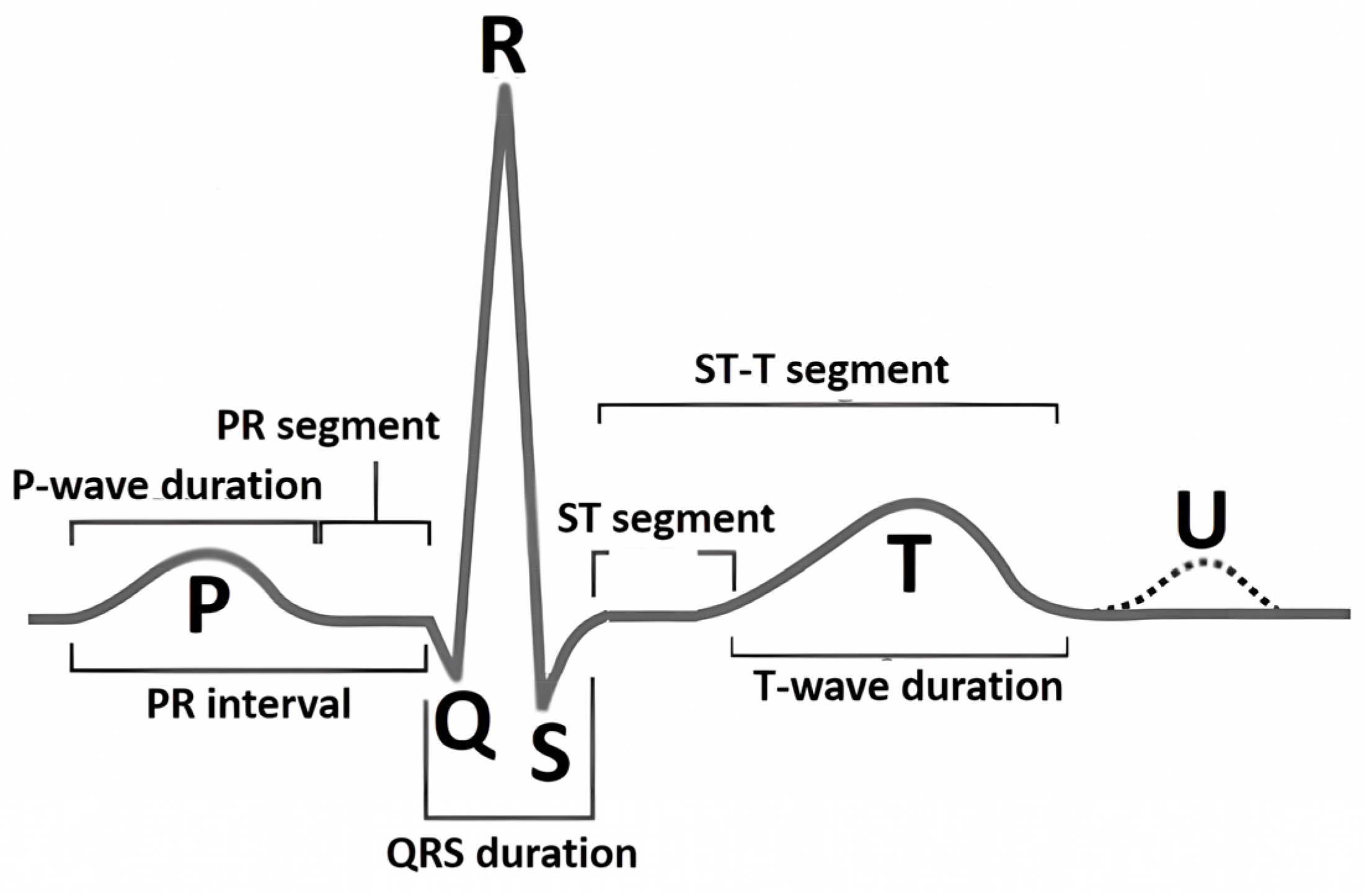
Figure 2.
This figure outlines a three-step ECG arrhythmia classification approach using XAI. It starts with ECG input and proceeds through R peak identification, arrhythmia classification, and result interpretation, resulting in classified ECG fragments. This approach integrates domain knowledge to improve diagnostic accuracy and interpretability for clinicians.
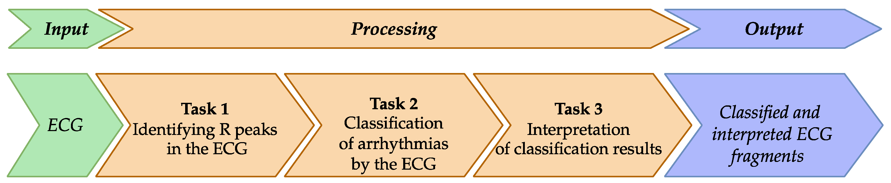
Figure 3.
This figure illustrates the R peak detection method in ECG analysis, consisting of three key steps: knowledge integration, CNN processing, and post-processing. This method leverages domain knowledge of the reference heart cycle to enhance R peak detection accuracy, producing precise R peak locations in the output.
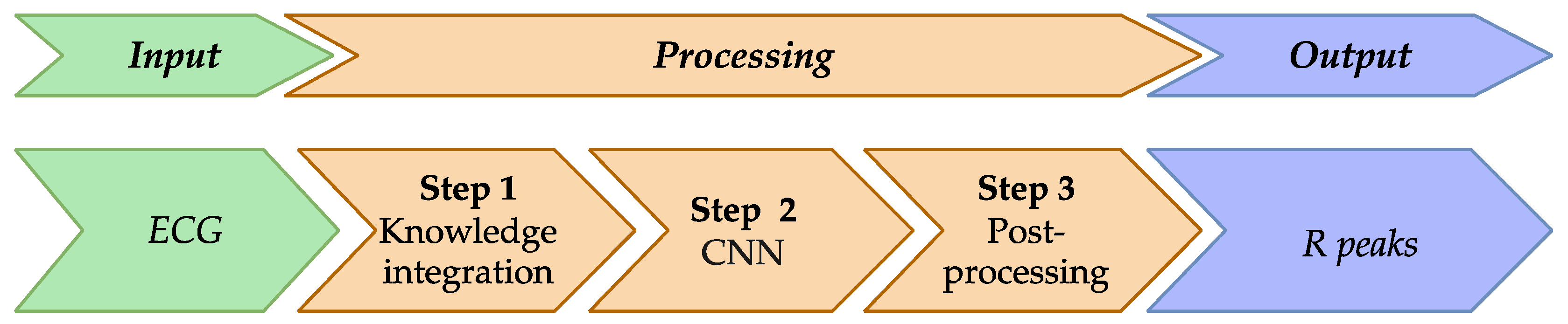
Figure 4.
This figure details Step 1 of the R peak detection method, focusing on integrating reference ECG knowledge. The process begins by analyzing 260 data points of the ECG to find the maximum deviation, representing the wave peak. If confirmed, knowledge integration is applied. The process skips 100 items after each peak to avoid redundancy until the end of the signal, generating a knowledge-integrated array K for further processing.
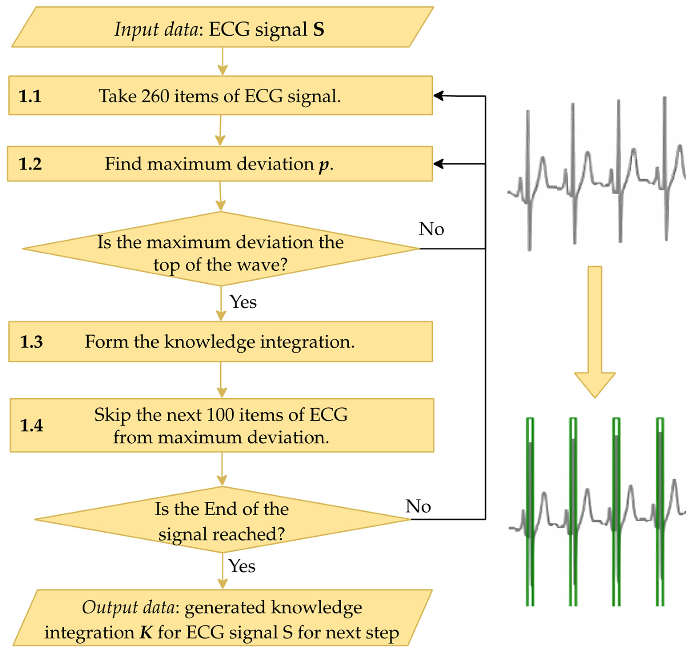
Figure 5.
A schematic that shows the integration of reference ECG knowledge into the current ECG. The green overlay highlights sections where knowledge integration occurs around R peaks, providing visual markers that aid in accurately identifying peak positions for improved signal analysis and arrhythmia detection.
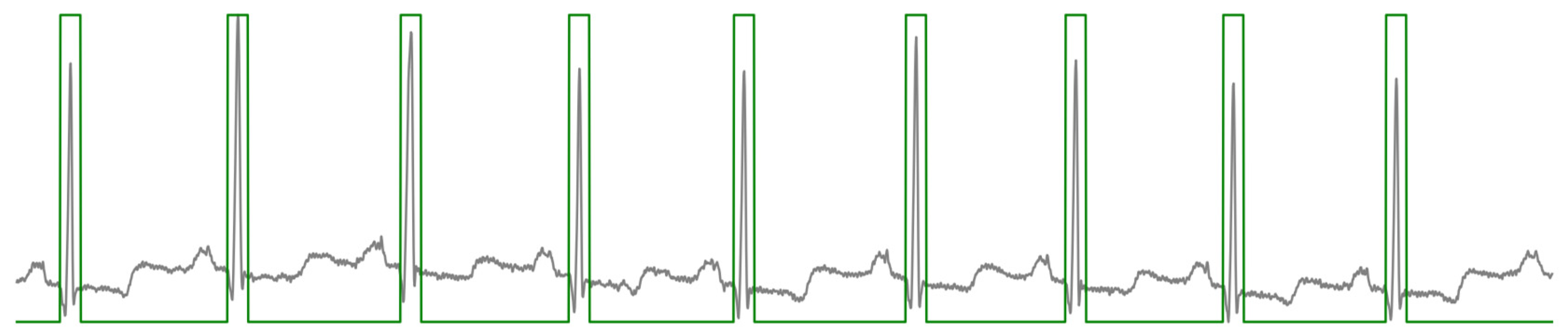
Figure 6.
This figure illustrates the post-processing steps for CNN-predicted R peak identification. Starting with CNN predictions, the process filters data, identifies the maximum prediction in each range, and saves it in an output array D. It iterates through the signal to create a comprehensive index array of R peak positions.
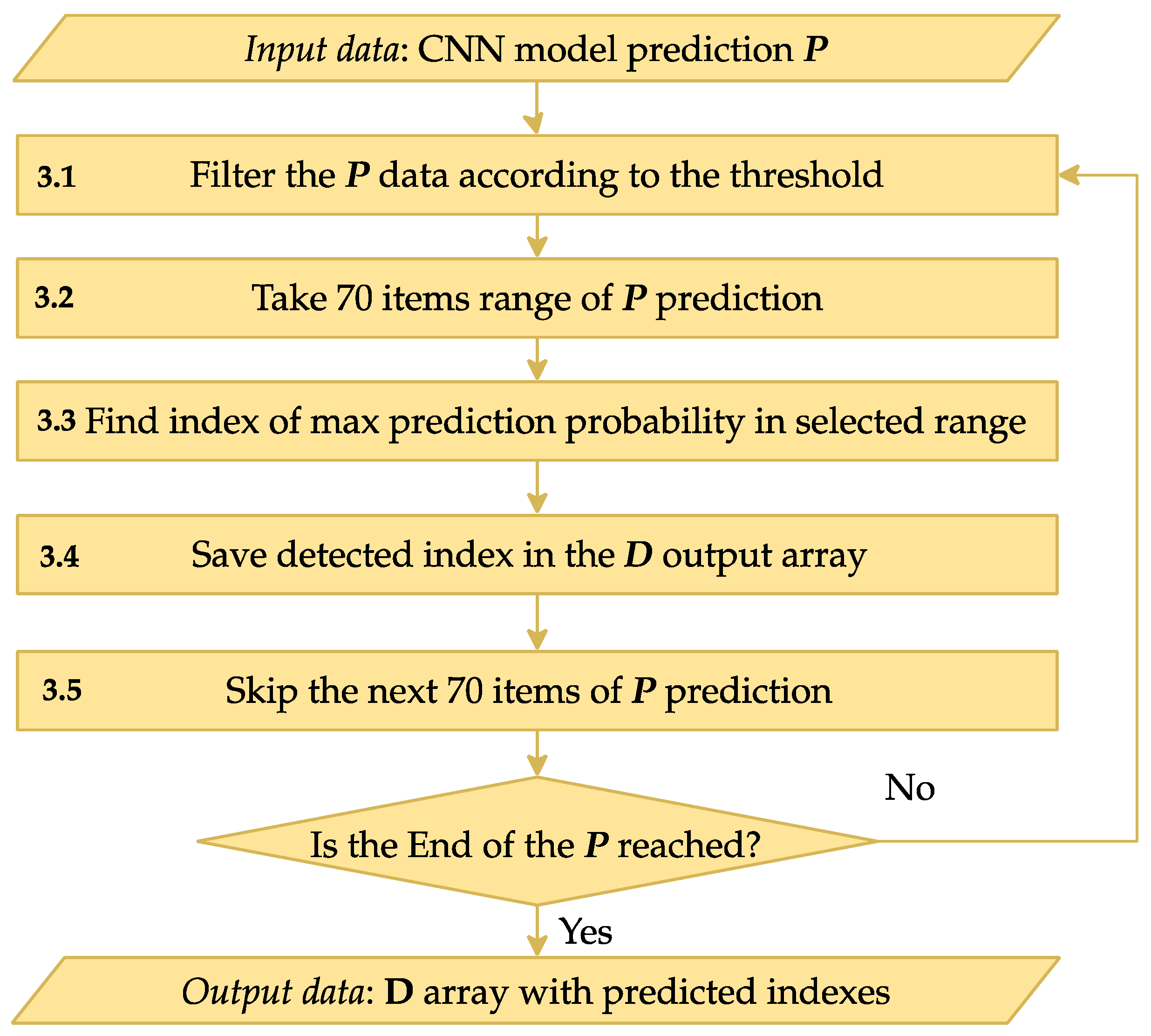
Figure 7.
This figure presents an ECG classification method for arrhythmia detection, beginning with ECG and R peak indices. The process involves splitting the ECG into fragments and using a CNN model to classify each fragment, resulting in predicted pathology labels for individual ECG segments to support clinical diagnosis.
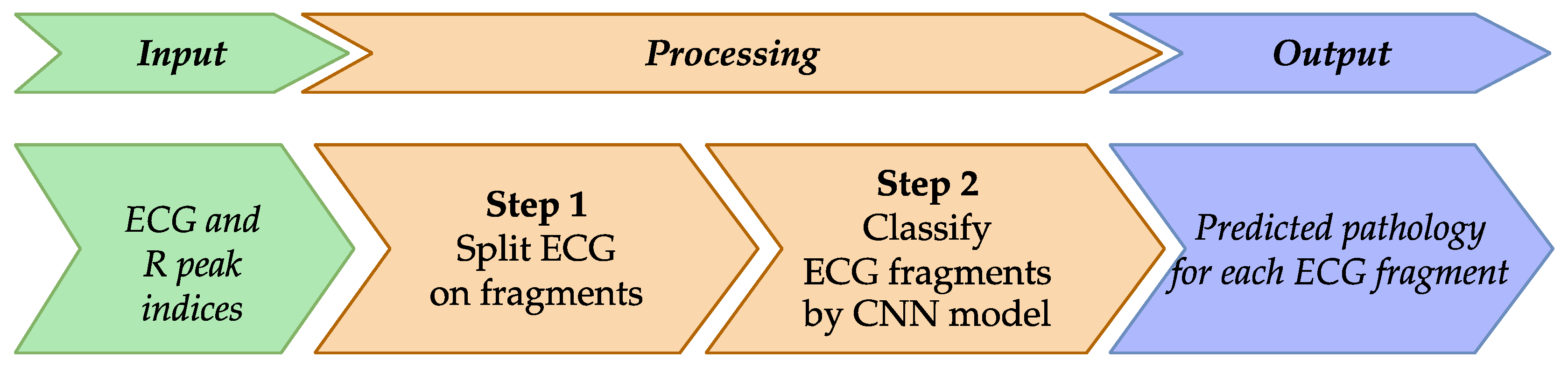
Figure 8.
This figure illustrates a step-by-step method for detecting specific features in a classified ECG fragment. Starting with a 700-length ECG segment, it empirically identifies the receptive region, analyzes the presence of features, and applies methods like formula-based verification, visualization, and ML or DL classification. Each step is designed to confirm or deny feature presence, with outcomes supporting clinical interpretation of ECG data.
Figure 9.
Training set samples for two ECG classes, comparing separation clarity in a designated zone of interest. Subfigures (a) and (c) illustrate cases without clear separation, (b) and (d) display distinguishable separation patterns in the interest zone. The cardio cycle being interpreted over each group is superimposed with a rectangle, highlighting the zone of interest and representing the relevant signal fragment.
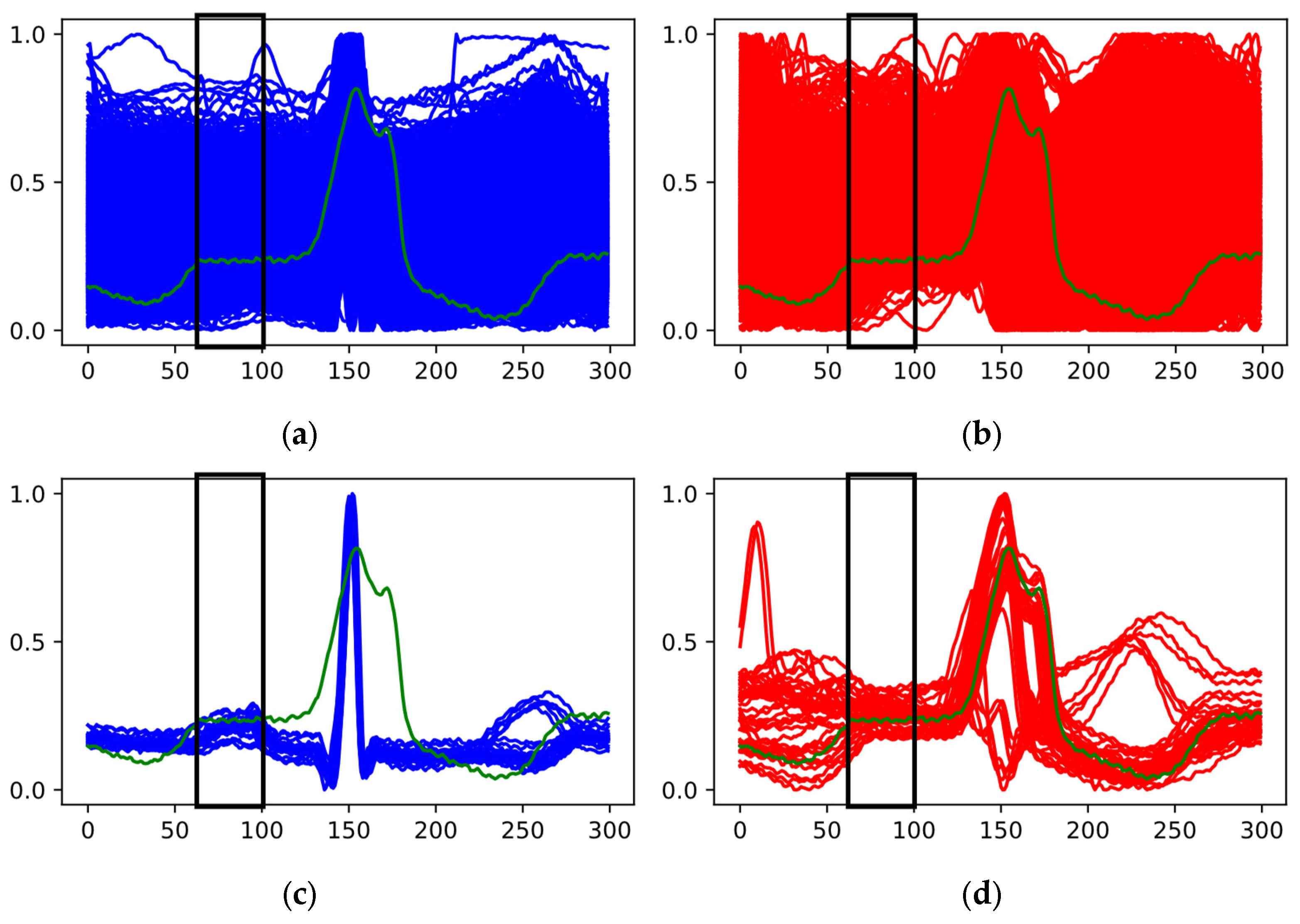
Figure 10.
The application of PCA on ECG fragments within the zone of interest. Red and blue clusters represent two distinct classes, highlighting areas of overlap and separation; green dot represents the target ECG.
Figure 10.
The application of PCA on ECG fragments within the zone of interest. Red and blue clusters represent two distinct classes, highlighting areas of overlap and separation; green dot represents the target ECG.
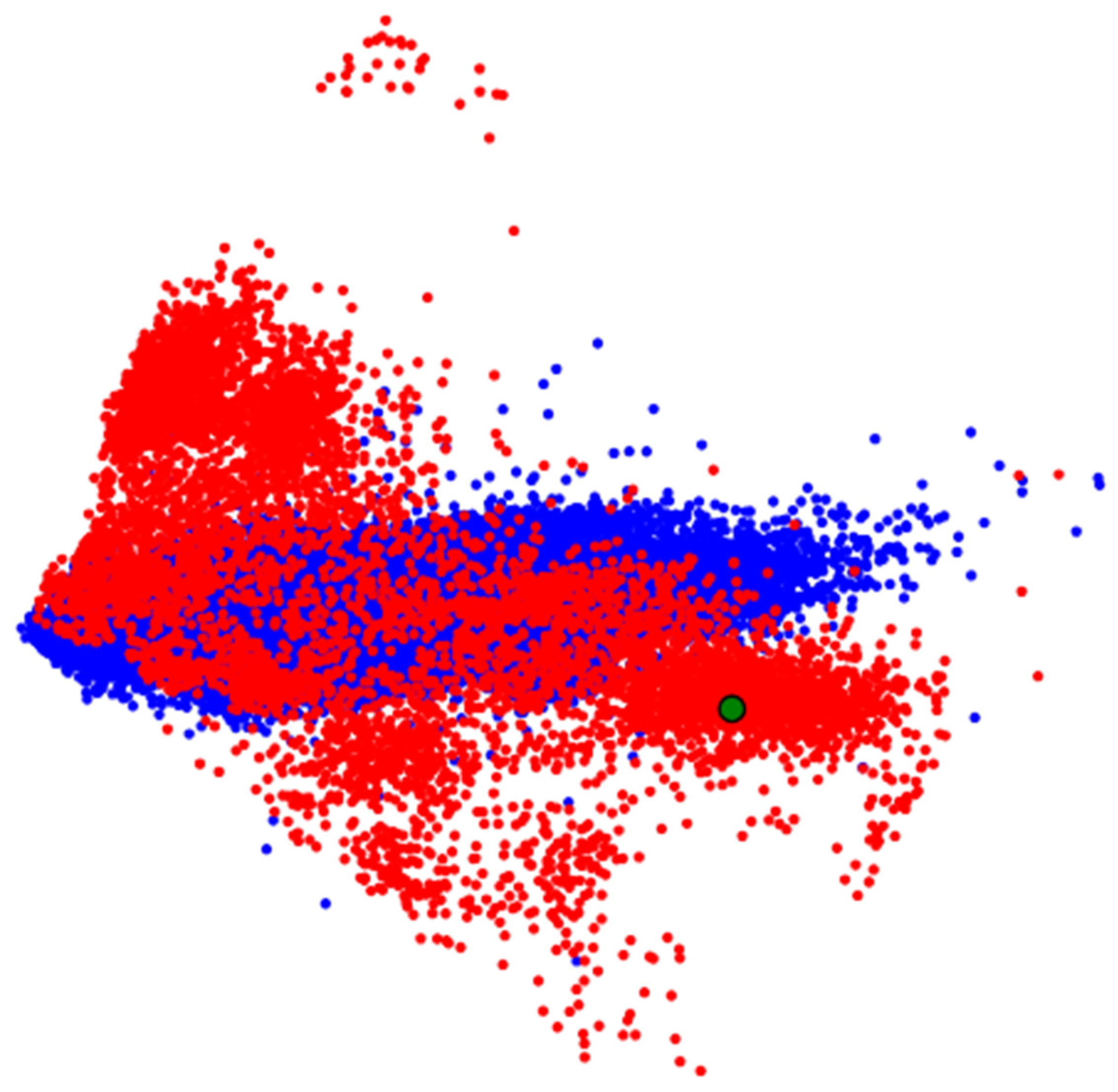
Figure 11.
Training and validation curves for accuracy (a) and loss (b) over 18 epochs. The rapid convergence of accuracy and reduction in loss indicate effective training with minimal overfitting, demonstrating the CNN model’s stability and generalizability for ECG classification tasks.
Figure 11.
Training and validation curves for accuracy (a) and loss (b) over 18 epochs. The rapid convergence of accuracy and reduction in loss indicate effective training with minimal overfitting, demonstrating the CNN model’s stability and generalizability for ECG classification tasks.
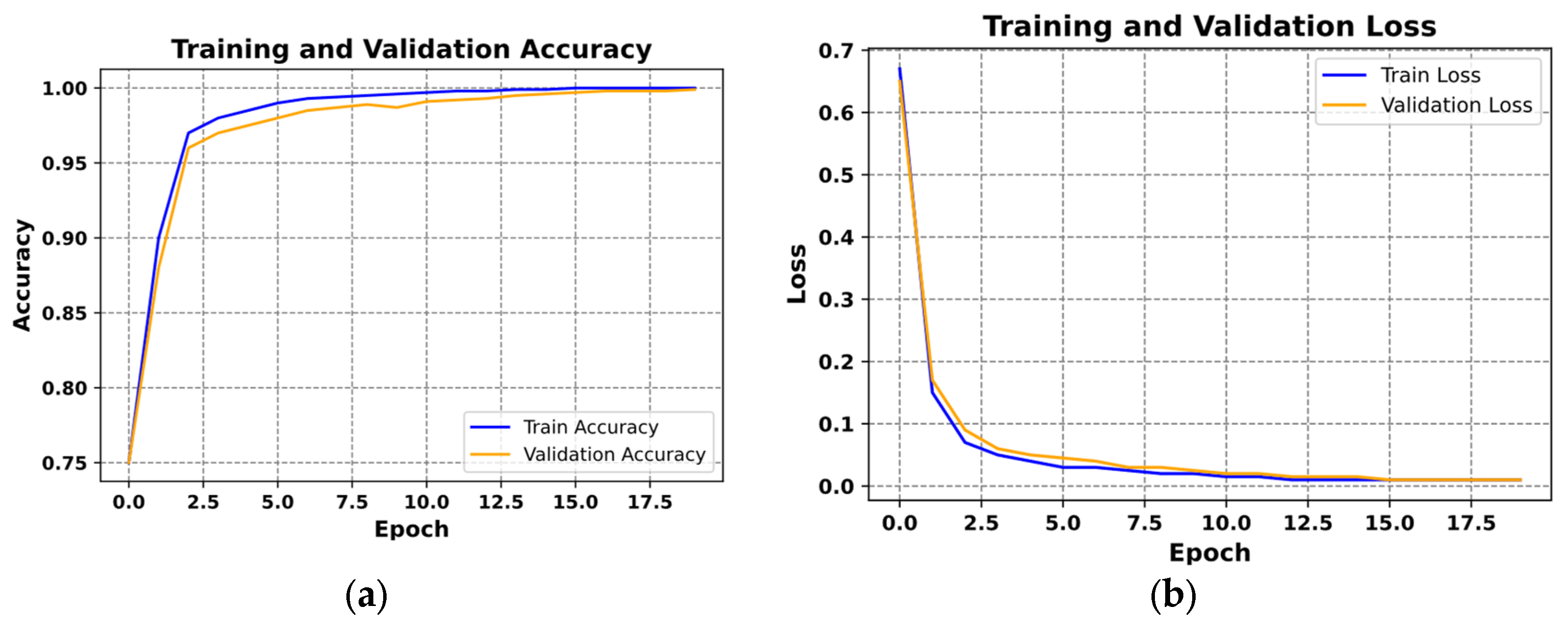
Figure 12.
ROC curves for a multi-class classification of ECG data, showing near-perfect AUC values (mostly 1.00), indicating high model performance. Minor deviations in classes 7 and 9 suggest slight inconsistencies in distinguishing these classes, reflecting model robustness overall.
Figure 12.
ROC curves for a multi-class classification of ECG data, showing near-perfect AUC values (mostly 1.00), indicating high model performance. Minor deviations in classes 7 and 9 suggest slight inconsistencies in distinguishing these classes, reflecting model robustness overall.
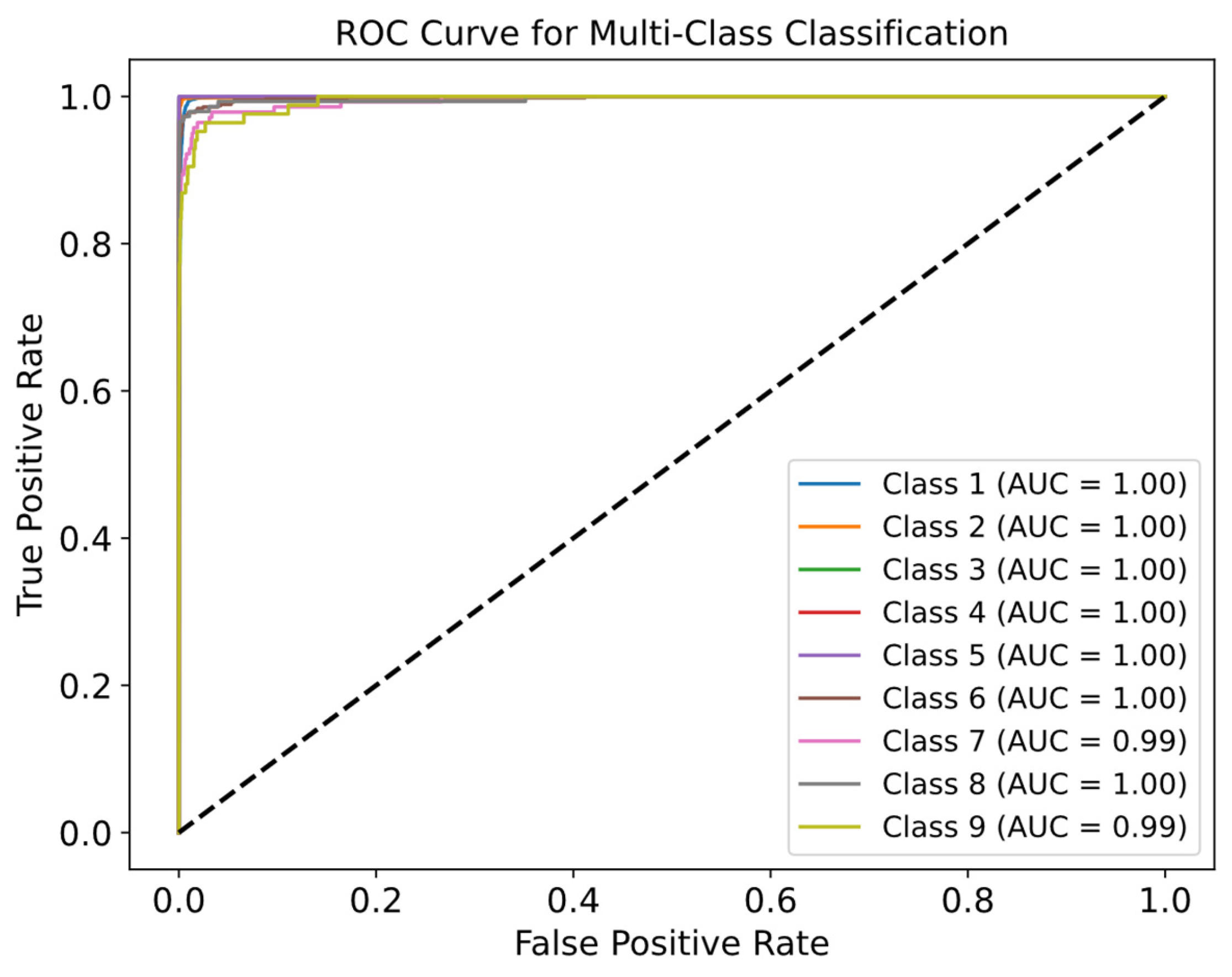
Figure 13.
This figure presents One-vs-One ROC curves for ECG classification, demonstrating high accuracy in class differentiation: (a) shows normal vs. others (AUC 0.99), (b) class 9 vs. 1 (AUC 1.00), (c) LBBB vs. RBBB (AUC 1.00), and (d) classes 5 vs. 4 (AUC 1.00).
Figure 13.
This figure presents One-vs-One ROC curves for ECG classification, demonstrating high accuracy in class differentiation: (a) shows normal vs. others (AUC 0.99), (b) class 9 vs. 1 (AUC 1.00), (c) LBBB vs. RBBB (AUC 1.00), and (d) classes 5 vs. 4 (AUC 1.00).
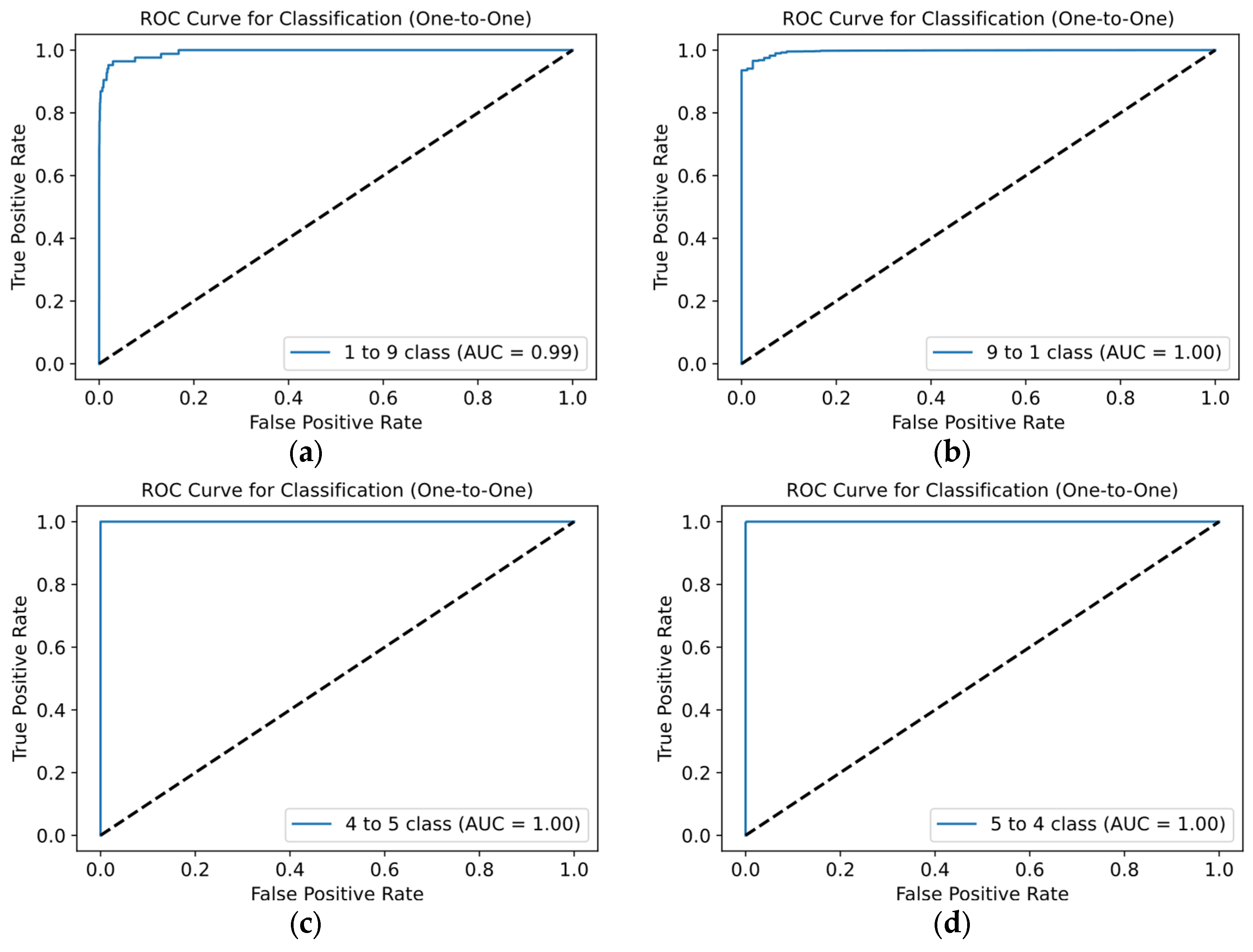
Figure 14.
A multi-channel ECG recording used in clinical trials, with annotations indicating normal cycles and those with PVC.
Figure 14.
A multi-channel ECG recording used in clinical trials, with annotations indicating normal cycles and those with PVC.
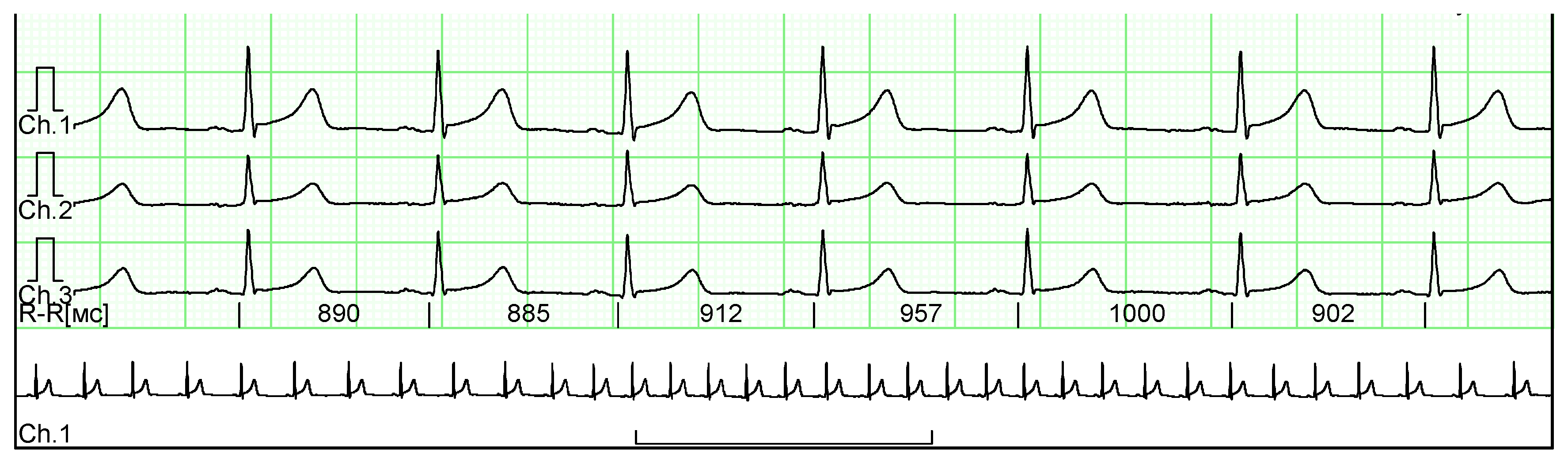
Figure 15.
This figure illustrates the process of splitting a multi-channel ECG image into separate channel-specific images. Each channel is isolated to enable focused analysis, facilitating the detection of specific patterns and anomalies within each individual ECG trace, such as PVC.
Figure 15.
This figure illustrates the process of splitting a multi-channel ECG image into separate channel-specific images. Each channel is isolated to enable focused analysis, facilitating the detection of specific patterns and anomalies within each individual ECG trace, such as PVC.
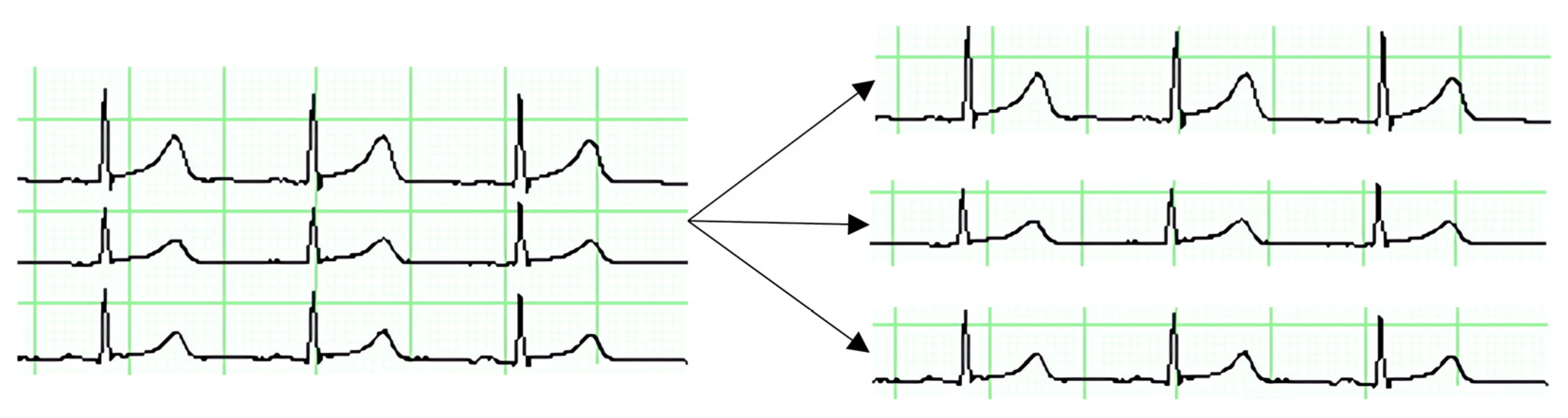
Figure 16.
This confusion matrix depicts the performance of the pathology classification model in clinical trials. Two Class 1 cycles were misclassified as Class 3, and one Class 3 cycle was misclassified as Class 1, indicating high but not perfect agreement.
Figure 16.
This confusion matrix depicts the performance of the pathology classification model in clinical trials. Two Class 1 cycles were misclassified as Class 3, and one Class 3 cycle was misclassified as Class 1, indicating high but not perfect agreement.
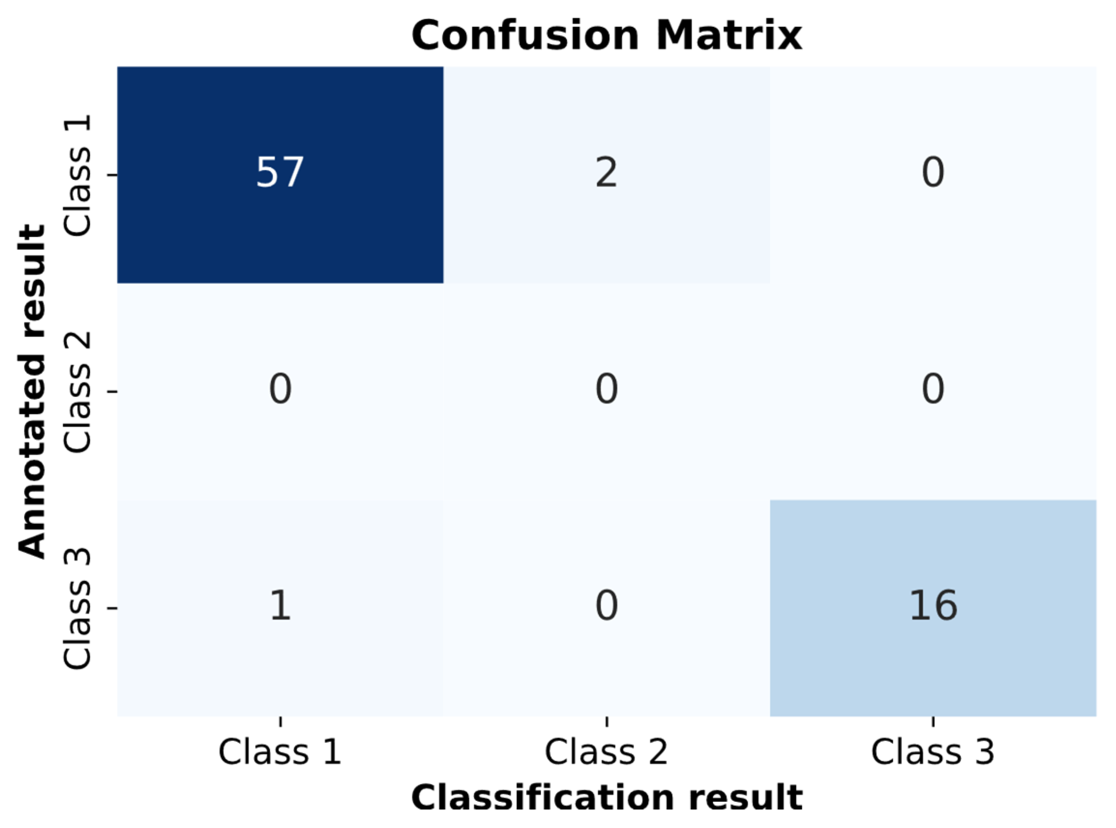
Figure 17.
This figure visually confirms specific pathology features in ECG cycles (a) a normal ECG cycle, (b) key peak markers, (c) ST-segment depression, and (d) a deformed QRS complex, providing clear visual evidence for classification interpretations based on distinctive signal characteristics.
Figure 17.
This figure visually confirms specific pathology features in ECG cycles (a) a normal ECG cycle, (b) key peak markers, (c) ST-segment depression, and (d) a deformed QRS complex, providing clear visual evidence for classification interpretations based on distinctive signal characteristics.
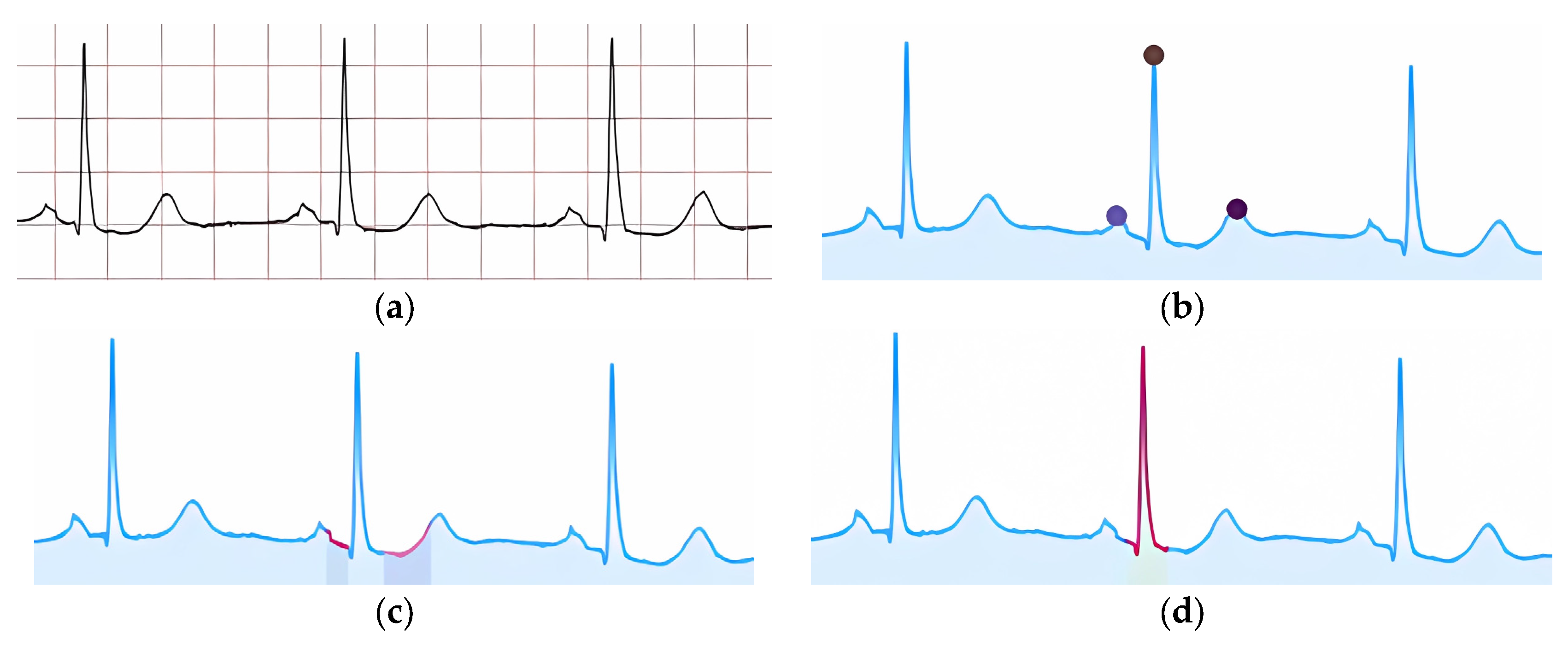
Figure 18.
Visual confirmation of ECG pathology features, focusing on (a) normal ECG, (b) extended QRS complex, and (c) discordant changes in the ST-T segment.
Figure 18.
Visual confirmation of ECG pathology features, focusing on (a) normal ECG, (b) extended QRS complex, and (c) discordant changes in the ST-T segment.
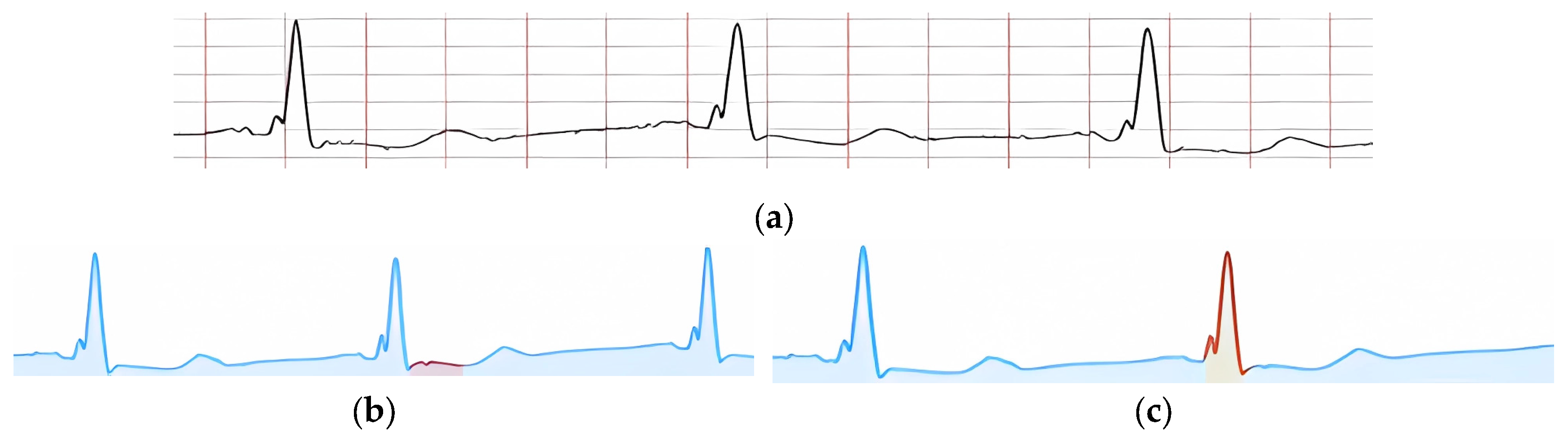
Figure 19.
Visual confirmation of ECG features, indicating LBBB, with the following specific waveform characteristics: (a) baseline ECG, (b) delayed ventricular activation, (c) ST segment elevation, and (d) widened QRS complex, assisting in precise pathology identification.
Figure 19.
Visual confirmation of ECG features, indicating LBBB, with the following specific waveform characteristics: (a) baseline ECG, (b) delayed ventricular activation, (c) ST segment elevation, and (d) widened QRS complex, assisting in precise pathology identification.
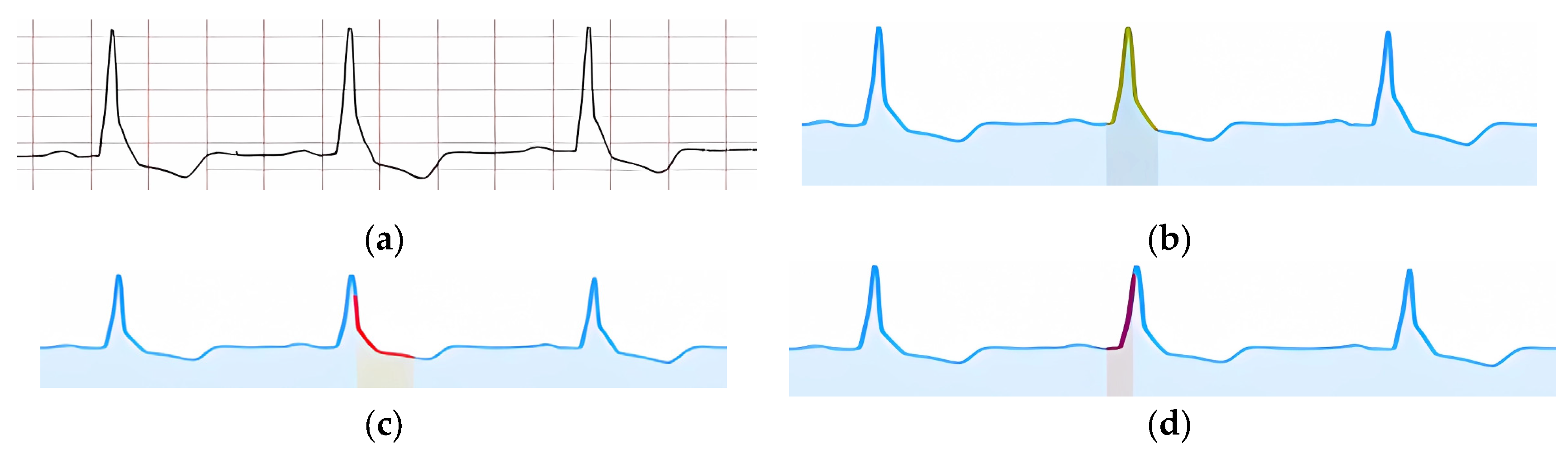
Figure 20.
Visual confirmation of “Ventricular Extrasystole” features in an ECG with the following key characteristics: (a) baseline ECG, (b) extended QRS complex, (c) absence of P wave, and (d) compensatory pause, facilitating accurate identification of ventricular arrhythmia.
Figure 20.
Visual confirmation of “Ventricular Extrasystole” features in an ECG with the following key characteristics: (a) baseline ECG, (b) extended QRS complex, (c) absence of P wave, and (d) compensatory pause, facilitating accurate identification of ventricular arrhythmia.
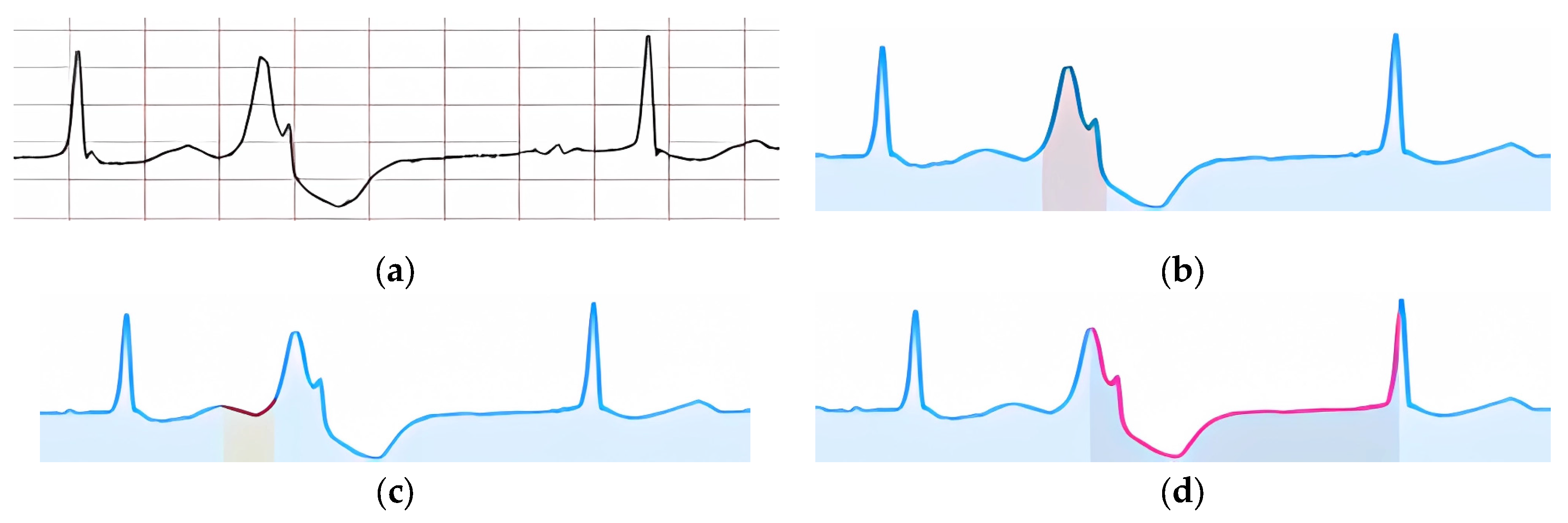
Figure 21.
This figure displays an ECG classified as “Fusion of Ventricular Extrasystole.” The waveform demonstrates characteristics of both normal and ectopic ventricular beats, indicative of fusion, where premature ventricular and normal impulses overlap, producing a unique hybrid beat.
Figure 21.
This figure displays an ECG classified as “Fusion of Ventricular Extrasystole.” The waveform demonstrates characteristics of both normal and ectopic ventricular beats, indicative of fusion, where premature ventricular and normal impulses overlap, producing a unique hybrid beat.
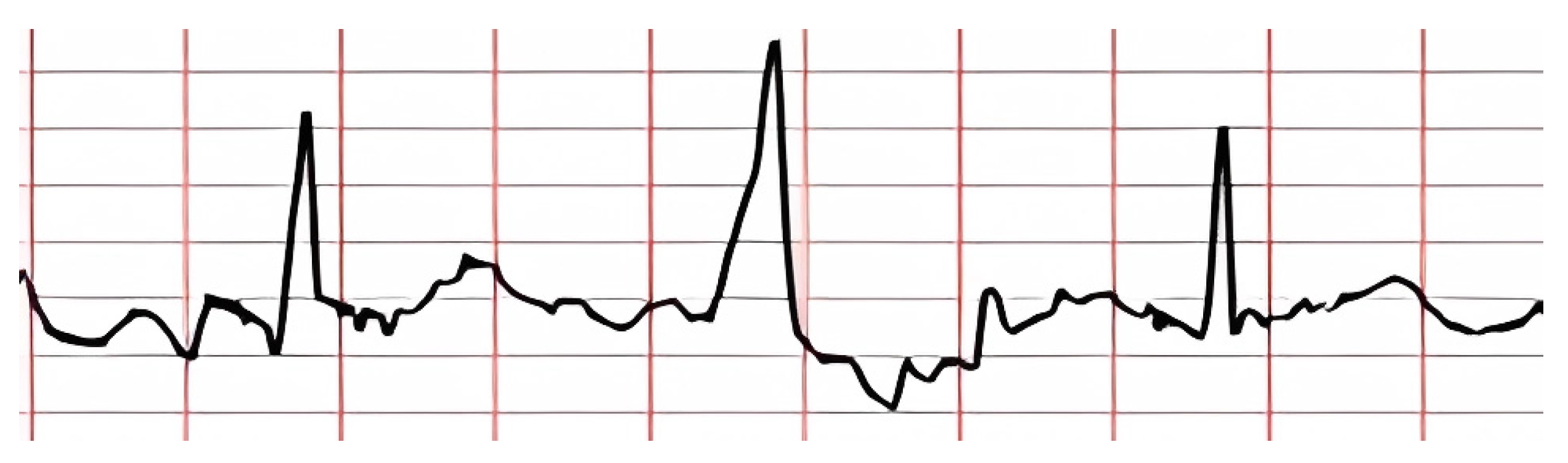
Figure 22.
Visual confirmation of features “Fusion of Ventricular Extrasystole,” specifically (a) extended and deformed QRS complex, (b) absence of the P peak, (c) lack of compensatory pause, and (d) ventricular extrasystole between normal cycles. These features aid in precise ECG pathology interpretation.
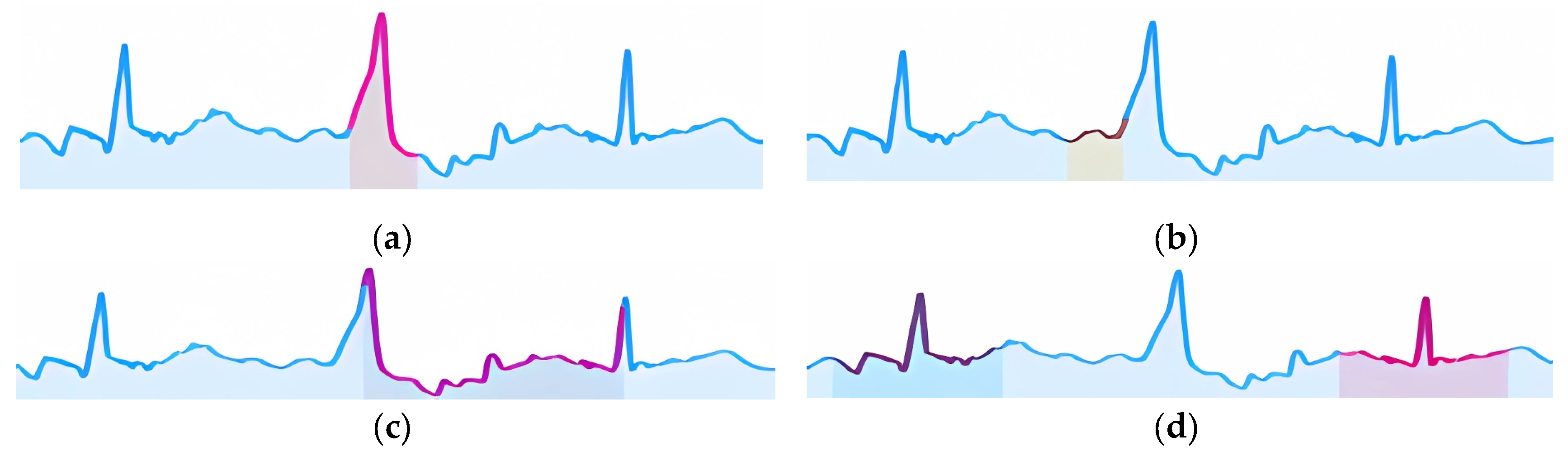
Table 1.
The distribution of ECG fragments across different datasets used in the study. Training data includes signals from MIT-BIH, QT, and CPSC-2020 databases, while testing data also includes MIT-BIH, QT, CPSC-2020, and a unique test set from the UoG ECG database.
Table 1.
The distribution of ECG fragments across different datasets used in the study. Training data includes signals from MIT-BIH, QT, and CPSC-2020 databases, while testing data also includes MIT-BIH, QT, CPSC-2020, and a unique test set from the UoG ECG database.
| Sample title | Database title | The number of fragments |
|---|---|---|
| Training data | MIT-BIH | 3,312 |
| QT | 2,484 | |
| CPSC 2020 | 33,195 | |
| Testing data | MIT-BIH | 828 |
| QT | 712 | |
| CPSC 2020 | 8,299 | |
| Unique test data | ECG Database—UoG | 438 |
Table 2.
A comparison of the proposed model’s performance on accuracy, precision, recall, and F1-score across multiple ECG databases (MIT, QT, CPSC-2020, UoG) against established approaches. Bold values indicate the highest scores.
Table 2.
A comparison of the proposed model’s performance on accuracy, precision, recall, and F1-score across multiple ECG databases (MIT, QT, CPSC-2020, UoG) against established approaches. Bold values indicate the highest scores.
| Database | Approach | Accuracy | Precision | Recall | F1-score |
|---|---|---|---|---|---|
| MIT | Zahid et al. [11] | 0.9999 | 0.9905 | 0.9858 | 0.9893 |
| NeuroKit2 [33] | 0.9997 | 0.9644 | 0.9340 | 0.9490 | |
| Rodrigues et al. [40] | 0.9992 | 0.8322 | 0.9491 | 0.8868 | |
| Koka et al. [41] | 0.9992 | 0.8938 | 0.8699 | 0.8817 | |
| Our | 0.9999 | 0.9921 | 0.9872 | 0.9890 | |
| QT | Zahid et al. [11] | 0.9999 | 0.9789 | 0.9778 | 0.9783 |
| NeuroKit2 [33] | 0.9997 | 0.9655 | 0.9410 | 0.9531 | |
| Rodrigues et al. [40] | 0.9991 | 0.7824 | 0.9427 | 0.8551 | |
| Koka et al. [41] | 0.9993 | 0.8866 | 0.8767 | 0.8816 | |
| Our | 0.9999 | 0.9803 | 0.9818 | 0.9819 | |
| CPSC-2020 | Zahid et al. [11] | 0.9999 | 0.9855 | 0.9927 | 0.9891 |
| NeuroKit2 [33] | 0.9997 | 0.9514 | 0.9514 | 0.9514 | |
| Rodrigues et al. [40] | 0.9989 | 0.7763 | 0.9212 | 0.8426 | |
| Koka et al. [41] | 0.9995 | 0.9232 | 0.8972 | 0.9100 | |
| Our | 0.9999 | 0.9862 | 0.9943 | 0.9897 | |
| UoG | Zahid et al. [11] | 0.9995 | 0.9838 | 0.8666 | 0.9215 |
| NeuroKit2 [33] | 0.9998 | 0.9932 | 0.9596 | 0.9761 | |
| Rodrigues et al. [40] | 0.9996 | 0.9083 | 0.9990 | 0.9515 | |
| Koka et al. [41] | 0.9994 | 0.9194 | 0.8968 | 0.9080 | |
| Our | 0.9996 | 0.9831 | 0.9010 | 0.9239 |
Table 3.
Average metrics for nine-class ECG classification.
| Metric | Precision | Recall | F1-score |
|---|---|---|---|
| Macro | 0.97 | 0.95 | 0.96 |
| Weighted | 0.99 | 0.99 | 0.99 |
Table 4.
Average metrics for ECG classification when excluding the “Others” class due to its underrepresentation and variability.
Table 4.
Average metrics for ECG classification when excluding the “Others” class due to its underrepresentation and variability.
| Metric | Precision | Recall | F1-score |
|---|---|---|---|
| Macro | 0.97 | 0.95 | 0.96 |
| Weighted | 0.99 | 0.99 | 0.99 |
Table 5.
A comparison of the proposed ECG classification method with AAMI-based classification approaches, highlighting superior performance across all metrics. Bold color indicates the highest value of each metric.
Table 5.
A comparison of the proposed ECG classification method with AAMI-based classification approaches, highlighting superior performance across all metrics. Bold color indicates the highest value of each metric.
| Approach | Number of groups |
Accuracy | Precision | Recall | F1-score |
|---|---|---|---|---|---|
| Hassan et al. [17] | 5 | 0.980 | 0.920 | 0.910 | 0.915 |
| Our | 0.993 | 0.970 | 0.940 | 0.965 | |
| Xu et al. [19] | 5 | 0.998 | 0.980 | 0.940 | 0.961 |
| Our | 0.993 | 0.960 | 0.940 | 0.950 | |
| Ahmed et al. [44] | 4 | 0.990 | 0.930 | 0.940 | 0.935 |
| Our | 0.993 | 0.960 | 0.940 | 0.950 | |
| Kumar et al. [45] | 5 | 0.987 | 0.989 | 0.939 | 0.963 |
| Our | 0.993 | 0.960 | 0.940 | 0.950 | |
| Mahmud et al. [46] (Signal) |
6 | 0.940 | 0.950 | 0.900 | 0.920 |
| Our | 0.993 | 0.960 | 0.940 | 0.950 | |
| Mahmud et al. [46] (Image) |
6 | 0.930 | 0.930 | 0.930 | 0.930 |
| Our | 0.993 | 0.960 | 0.940 | 0.950 |
Table 6.
A comparison of the proposed ECG classification method with existing approaches for atomic pathology classification, showing consistently high metrics. Bold color indicates the highest value of each metric.
Table 6.
A comparison of the proposed ECG classification method with existing approaches for atomic pathology classification, showing consistently high metrics. Bold color indicates the highest value of each metric.
| Approach | Number of classes |
Mutual classes |
Precision | Recall | F1-score |
|---|---|---|---|---|---|
| Liu et al. [18] | 4 | 4 | – | 0.993 | – |
| Our | 0.993 | 0.995 | 0.994 | ||
| Degirmenci et al. [20] | 5 | 5 | 0.995 | 0.997 | 0.992 |
| Our | 0.993 | 0.997 | 0.995 | ||
| Rohmantri et al. [21] | 8 | 7 | 0.973 | 0.893 | 0.927 |
| Our | 0.970 | 0.950 | 0.960 | ||
| Ullah et al. [22] | 8 | 6 | 0.985 | 0.977 | 0.981 |
| Our | 0.988 | 0.984 | 0.986 | ||
| Yang et al. [47] | 6 | 6 | 0.991 | – | 0.966 |
| Our | 0.988 | 0.984 | 0.986 |
Disclaimer/Publisher’s Note: The statements, opinions and data contained in all publications are solely those of the individual author(s) and contributor(s) and not of MDPI and/or the editor(s). MDPI and/or the editor(s) disclaim responsibility for any injury to people or property resulting from any ideas, methods, instructions or products referred to in the content. |
© 2024 by the authors. Licensee MDPI, Basel, Switzerland. This article is an open access article distributed under the terms and conditions of the Creative Commons Attribution (CC BY) license (https://creativecommons.org/licenses/by/4.0/).
Copyright: This open access article is published under a Creative Commons CC BY 4.0 license, which permit the free download, distribution, and reuse, provided that the author and preprint are cited in any reuse.


