
Submitted:
07 July 2025
Posted:
08 July 2025
You are already at the latest version
Abstract
Cardiovascular diseases (CVDs), which remain globally one of the most common causes of death, are usually diagnosed based on the electrocardiogram (ECG) signal. To support human experts, modern deep-learning models are used for CVD classification problems as an early warning. This article proposes a novel multi-branch architecture focused on processing various modalities of the ECG signal in parallel branches replacing typical single-input architectures. Each branch is given separate input in the form of the raw signal, domain knowledge, the wavelet transform of the signal, or the signal with drift removed. The proposed method is based on deep-learning core models that can incorporate various modern neural networks. It was thoroughly tested on N-BEATS, LSTM, and GRU neural networks. The proposed architecture allows the retention of the speed of the neural network. At the same time, the combination of independently computed branches improves model performance, which finally exceeds the performance obtained by classical single-branch architectures.
Keywords:
ECG classification
; cardiovascular diseases
; neural network
; N-BEATS
; RNN
; GRU
; LSTM
1. Introduction
Cardiovascular diseases (CVDs) are one of the most common causes of death globally. An electrocardiogram (ECG) signal representing the heart’s electrical activity is widely used to detect and classify cardiac arrhythmias. Visual inspection of the ECG waveform allows anomalies to be detected. It is crucial in the early stages of heart disease when symptoms occur only occasionally. In such cases, continuous monitoring by wearable devices and an automatic classification process increase the chances of proper detection. To increase the efficiency of ECG analyses, methods for automatic detection of ECG abnormalities are used instead of a physician visually reviewing the ECG waveform periodically. This way, when the algorithm detects disease signals, it classifies them, and the doctor can be notified.
Originally, algorithms based on morphological features and classical signal-processing techniques were commonly used. However, these solutions turned out to be insufficient, as the ECG waveform’s morphological characteristics can have high variability between different patients and are susceptible to interference during measurement [1,2]. Nowadays, deep-learning-based algorithms using recurrent neural networks (RNNs) and convolutional neural networks (CNNs) dominate the field [1,3,4,5]. Recent publications prove hybrid or extended variations of said architectures [6,7] to excel in the ECG analysis task. Another approach gaining traction is the use of attention-based models, where by employing convolutional layers combined with attention, the CNN autonomously extracts detailed morphological and temporal patterns from raw multi-lead ECG data – often removing the need for handcrafted features while delivering higher accuracy and robust cross-dataset performance [8,9].
As ECG classification and prediction are problems in time-series analysis, one of the most commonly used classifiers in that field is the Long Short-term Memory (LSTM) network [10]. The LSTM network is known for its ability to learn long-term dependencies from sequential data, which allows it to be leveraged to profit architectures focusing on both temporal changes and detailed signal artefacts [11]. Still, time-series forecasting continues to be a pivotal challenge in the field of machine learning, and despite the rapid evolution of contemporary algorithms, classical statistical methodologies are still commonly used. One of the interesting new solutions is a hybrid approach integrating a neural residual / attention-extended LSTM architecture with the conventional Holt-Winters statistical model augmented by learnable parameters that have gathered increasing attention [12]. Another new solution is Neural Basis Expansion Analysis for Interpretable Time Series (N-BEATS) [13,14] – one of the newest neural networks used primarily for forecasting time series. In [15], N-BEATS, which was previously used only for forecasting, was proposed to diagnose cardiac problems and compared with commonly used LSTM and GRU networks for such problems. N-BEATS achieved similar results in the experiments and worked exceptionally well for a low number of ECG leads.
In [16,17], a two-branch architecture with two blended sub-networks and wavelet analysis, was shown as superior to common N-BEATS, LSTM and GRU architectures. In this article, this idea is further developed into a new architecture model and instead of adding domain knowledge or other information as a single input with ECG signal, a multi-branch architecture is proposed with up to 6 branches containing different inputs, like raw signal, domain knowledge, the wavelet transform of the signal or drift removal. Multi-branch architecture containing independent branches proved to obtain better results in all tested scenarios, improving the overall performance of neural networks. The paper uses three basic neural networks (LSTM, GRU, N-BEATS) used interchangeably. For the sake of clarity they will be denoted as core networks.
2. Proposed Approach
2.1. Multi-Branch Architecture
In this paper, we follow the approach from [17], where a concept consisting of core networks with two blended sub-networks and wavelet analysis was introduced. Here we propose a novel architecture model. Instead of combining domain knowledge or other information with the ECG signal into a single input, multiple inputs are prepared individually (as shown in Figure 1), and a complex network architecture with six independent branches is proposed, each containing a core network and dedicated input (as shown in Figure 2). The branches of the model are denoted further in this paper as .
Popular solutions from state-of-the-art publications were used as inputs for individual architectural branches. The Raw ECG signal used as input on every branch was subject to denoising, which was performed using wavelet thresholding. The wavelet of choice is Daubechies, the most popular choice for denoising ECG signals [18]. Signals from different datasets were resampled to a common target frequency of 500 Hz (more on the process in Section 3.1). As shown in Figure 1 for computing inputs to branches, baseline drift was removed from a denoised signal with the SNIP algorithm. In order to compute the input to the branch, nonlinear baseline wandering was removed from the denoised signal. The inputs are presented in more detail later in this section.
The data individually preprocessed make the input for dedicated branches consisting of one or more core network blocks with FC (fully connected) layers. Dropouts are added in order to prevent overfitting and improve generalisation [19]. Outputs of those branches are concatenated and used as input for a fully connected neural network layer (FC) to produce probabilities of all output classes. The model of the multi-branch architecture is shown in Figure 2.
Different modalities of the original signal, obtained by described above preprocessing, extends the information resource used to identify the particular signal sample. The details concerning branches is given below.
- The branch contains the processed ECG signal. As the region surrounding the R peak is critical for diagnosing cardiovascular diseases (CVDs) [16], an R peak detection algorithm is employed for signal segmentation. In this study, we utilized the commonly used Pan-Tompkins algorithm [20] to facilitate both R peak detection and the subsequent segmentation process. Digital ECG recordings were divided into 3-second-long windows surrounding detected peaks, with exactly 1s of the signal prior to peak appearance and 2s afterwards.
- The branch contains information that encapsulates both time and frequency domain information. 4th level wavelet decomposition using type second Daubechies wavelet [21] was performed on the downsampled (by a factor of 2) ECG signal. Obtained approximation and detail coefficients are concatenated to form an input vector , where is an approximation vector and are detail coefficients.
- The branch represents professional expertise and domain knowledge of medical authorities [22] defined as indexes and statistics calculated to gain insights, which could potentially be hard to learn by the network. We employed McPhie, Romhilt, Cornell, Lewis and Sokolov-Lyon indexes as well as Cornell product, cardiac rhythm origin (split into two indicators of horizontal and vertical directions), electrical heart axis, and QRS complex statistics like QRS duration, R-S slope duration, notched QRS complex analysis, missing QRS, missing P-wave analysis and heart beats per minute [23,24,25,26]. As most of the aforementioned indicators relate to a single QRS complex across different leads and multiple heartbeats may appear during the 3-second window, we pad each index vector to allocate up to 25 beats. It forms an input matrix of shape 12x256, as shown in Figure 3.
- The branch contains the principal component analysis (PCA) [27] computed on the vector of the combined downsampled version of input (a raw ECG signal), concatenated with input (wavelet coefficients) and input (domain knowledge representation).
- The branch contains ECG signal (as in branch) with slow baseline drift [28] removed in preprocessing. Slow baseline drift removal removes inherent human- and hardware-related predicaments from the recordings.
- The branch contains ECG signal (as in branch) with nonlinear baseline wandering [29] removed in preprocessing. Nonlinear baseline wandering is a technique used to remove sudden signal disruptions and other anomalies (for example, moving the electrode) caused by the patient or the medical personnel from the recordings.
The architecture leverages the advantages of the bootstrap mechanism combined with different input perspectives. By merging the outputs of independent branches, which do not share insights in respective inputs of data, in the Blend layer, the proposed multi-branch architecture enhances the cumulative performance, improving classification outcomes with minimal increase in the total complexity of the solution.
2.2. Core Networks
Each branch consist of the core network, which is the main processing engine (see Figure 2). As the core network one may use different deep-learning models. Data processing by the core network can be performed multiple times on more than single block of the same network, which increases model efficiency, which was shown in [17]. In our research we tested three models used as the core network: LSTM, GRU and NBeats.
The LSTM architecture, proposed in 1997 by Hochreiter and Schmidhuber [30], is a variant of recurrent neural network in which each memory cell holds its state with a self-connection (the constant error carousel), while trainable input and output gates decide when to write new data into the cell and when to release its contents. By guaranteeing uninterrupted gradient flow over extended sequences, this design overcomes the vanishing gradient problem and lets the model selectively retain or discard information, making it exceptionally well-suited for capturing long-range dependencies in sequential data.
Gated recurrent unit (GRU) was first introduced in 2014 by Cho et al. [31]. While retaining LSTM’s gated approach to managing information flow, the GRU relies on just two gates - an update gate that blends the previous hidden state with a newly proposed activation and a freshly introduced reset gate to control incorporation of previous state—eliminating separate memory cells, lowering parameter count, easing training, yet still ensuring robust gradient propagation for capturing long-range dependencies.
In [13], Oreshkin et al. introduced the N-Beats architecture, designed explicitly for interpretable time series forecasting for the architectural model. The cornerstone of this framework is a multi-layer fully connected (FC) network, wherein non-linearities are introduced via the ReLU activation function. This network is tasked with predicting the basis expansion coefficients in both the forward (forecast) and backwards (backcast) directions. Individual blocks are systematically arranged into stacks through a doubly residual stacking strategy, potentially incorporating layers that share both backcast and forecast functionalities. The learned signal waveform represented by backcast is then removed from the original signal, and the result is passed further to the next block. Thanks to that, successive blocks learn to interpret exclusive parts of the signal. This hierarchical aggregation of forecasts facilitates the construction of a remarkably deep neural network while preserving the interpretability of its output and leveraging the benefits of the recurrent-like architecture.
3. Experiments
3.1. Datasets
Our experimental analysis utilized combined training dataset comprising over 88,000 annotated twelve-lead ECG recordings originating from six publicly available sources [32,33,34,35,36,37] as shown in Table 1. These recordings exhibit considerable variability in duration, ranging from 5 seconds to 30 minutes, and in sampling frequencies, including 250 Hz, 257 Hz, 500 Hz, and 1000 Hz. Notably, the majority of the samples are 10 seconds and recorded at 500 Hz. As such, signals with a sampling frequency lower than 500Hz were interpolated, and signals with a sampling frequency of 1000Hz were downsampled to match the target of 500Hz. Each of the six datasets encompasses 26 scored classes, comprising normal rhythm and 25 cardiac abnormalities, and up to 104 unscored classes. The heterogeneity in label quality and the presence of inaccuracies within these datasets contribute to the complexity of the challenge. The discussed sets have a signal from 12 ECG leads, and the analysis of such signals is used in the work because it provides the best results. However, due to the different quality of the sets, in order to protect the core networks from incorrect signals (where some leads are zeroed or lost in part of the signal), at the stage of pre-processing within the domain knowledge vector, marking of erroneous QRS readings and distances between peaks is used. The applied pre-processing allows the use of the architecture of both sets, containing full 12-lead ECG signals as well as those subject to external interference, leading to unsuccessful reads.
For comparative analysis of results, we employed cross-validation techniques by partitioning the entire dataset into five folds for training and testing purposes. Network weights were initialized using a fixed seed to ensure consistent randomization of the validation dataset for each training iteration, facilitating the selection of the optimal number of training epochs. The early stopping technique applied to the validation dataset guided the determination of epochs for a given training set. Subsequently, the model was trained across all training data within each fold, utilizing the initialized network weights from the fixed seed. As accuracy is not a feasible measure for the problem of multi-label classification, model performance was evaluated by calculating the average F-measure, and the challenge metric (see Section 3.3 for details) used in the CinC 2021 challenge.
3.2. Scenarios
To thoroughly verify the capabilities of the proposed solution, we introduced six scenarios described below.
- Scenario A — The first set of experiments was performed to establish the benchmark results and obtain a starting baseline for further comparison. We used a single-branch architecture and tested all branches separately, using only the LSTM (as the most often used) architecture as the core network. The basis of this scenario is an extension of the work published previously [17]. In our experiments, we employed a pruned ECG signal sample of length 0.7s (0.2s before the peak and 0.5s after the R peak).
- Scenario B — The second experiment tests possible differences between core network architectures working on different branches. As such, for each of the core networks, tests of single branches were performed for four branches: and . Omitted in the experiment were the branches , as domain knowledge alone proved to be inefficient, and , because branch baseline drift removal worked better. An enhanced input signal window (3s of signal) was used, and dropout layers were added.
- Scenario C — core network multi-branch architectures were tested with dropout layers embedded in the model. This comparison aimed to check if the combination improves model performance despite some branches offering no performance increase alone when all inputs are presented independently. This way, it can be checked if different perspectives (in the form of differently prepared independent inputs) can provide some improvement, even when such input alone works worse than the raw ECG signal.
- Scenario D — During this set of experiments, we measured and compared the performance of deeper architectures with an increased number of neurons in hidden layers. Multi-branch architecture was used for each of the core networks.
- Scenario E — In the third scenario, we test a multi-branch architecture with LSTM only with and without dropout layers and different pruning approaches. The goal was to establish a strategy to increase the network’s generalizing capability and improve overall performance while reducing the risk of overfitting.
- Scenario F — This experiment is an ablation study. The aim is to verify whether the exclusion of a given single branch from the initial complete set of six branches would change the overall performance of the architecture. Thus, it can be checked if any information from one of the independent branches could be considered excessive and removed to increase the architecture’s performance.
- Scenario G — Based on the results from scenarios D and E, additional tests on all three larger core networks were conducted, using different pruning strategies to check if the results from scenario D can be improved by applying different pruning techniques, especially for the underperforming networks.
3.3. Measuring the Performance
Following related papers submitted during the CinC (Computing in Cardiology) 2021 Challenge (now George B. Moody PhysioNet Challenge), to score results in a way that would allow comparing results to other state-of-the-art approaches, we apply a metric proposed by the CinC Challenge organizer.
As in paper [40], the following notation is used: is a set of m distinct diagnoses for a database of n recordings. is a multi-class confusion matrix where is the normalized number of recordings in a database that were classified to class but originally belonged to class . Different entries have assigned different weights defined in [40] based on the similarity of treatments or differences in risks. The score is a generalized version of the traditional accuracy metric. Finally, this score is normalized so that a classifier that always outputs the true class or classes receives a score of 1, and an inactive classifier that always outputs the normal class receives a score of 0:
where is the score for the inactive classifier and is the score for the ground-truth classifier.
The challenge metric was proposed for the complex multi-label classification problem of 26 different CVDs. It includes a matrix of weights that states how harmful misclassification is between each pair of diseases. One of the aims stated in the [40] is that a classifier that returns only positive outputs will typically receive a negative score, i.e., a lower score than a classifier that returns only negative outputs, reflecting the harm done by false alarms.
3.4. Results
The experiments were performed on computational servers with a 24-core processor clocked at 3.2 GHz, 256 GB RAM clocked at 3.2 GHz, and four NVIDIA Quadro RTX 5000 ADA 32 GB GPUs.
To thoroughly test the proposed approaches we performed experiments in 6 scenarios, which are described below.
- Scenario A – a test of single-branch architecture with LSTM as the core network. Table 2 shows results for six different branches (different data inputs) tested separately. The core network was configured with two hidden layers, with seven neurons each. As can be seen, branches perform worse than the baseline raw signal ( branch), while branches and obtain better results.
- Scenario B – tests possible differences between core network architectures working on different branches. Single branch tests were performed for branches , comparing LSTM, GRU, and N-BEATS architectures, and the results are provided in Table 3. Omitted in the experiment were the branches , as in Scenario A, domain knowledge alone proved to be inefficient, and , because branch baseline drift removal worked better. Each of the core networks was configured with two hidden layers, with seven neurons each. An enhanced input signal window (3s of signal) was used, and dropout layers were added. Dropout is a regularization technique for neural networks that prevents overfitting by randomly setting a subset of activations to zero during training, aiming to reduce co-adaptation of neurons, improving generalization [41]. Similarly to the experiment from scenario A, also in this scenario, the best results were achieved for the and branches. The obtained results were relatively consistent across all core networks, but it is worth noting that GRU tended to have the highest variance for branches, which gave the best results. Also, the addition of a dropout layer (not used in Scenario A) and larger signal window improved the LSTM network’s results of the branch so that they were almost the same as for the and for this network, only gave much better results.
- Scenario C – test comparing the multi-branch architectures of core networks. LSTM, N-BEATS, and GRU networks were used with a full six-branch architecture with a dropout layer and 5% pruning each epoch. Each of the core networks was configured with two hidden layers, with seven neurons each. The experiment shows that a full multi-branch architecture obtains better results for the 12-lead ECG signal (Table 4) than an architecture based on any of the single branches (Table 3), for each of the core networks. As can be seen, both GRU and LSTM achieved the same results in this scenario, with GRU being slightly faster and having more consistent results.
- Scenario D – tests how core networks performed after size increase. The network from Scenario C is modified, and two hidden layers of size 7 were changed into two hidden layers of size 11. The same dropout layer and 5% pruning each epoch are used. As can be seen in Table 5, despite an increase in network size, the time needed for classification was almost the same, while both the F-measure and challenge score for the two networks (N-BEATS and LSTM) significantly improved. An interesting observation is the worsening of the results of the GRU network, which obtained slightly worse results. The same result was obtained when the experiment was repeated. A careful inspection of the network weights showed that the weights for two branches ( and ) were practically zeroed within this architecture.
- Scenario E – test prune and dropout strategies on LSTM core network. The test is conducted on the multi-branch network with all six branches, and results are shown in Table 6. The core network was configured with two hidden layers, with seven neurons each. The best results were achieved for two configurations, both with an added dropout layer, in one case without pruning, and in the other with 20% L1 regularisation performed once. Other solutions, with the exception of one-time random 20% pruning, which considerably worsened the results, obtained the same or only slightly better results than the lack of prune and dropout.
- Scenario F — Results of an ablation study (single branch exclusion to check if any information can be considered excessive and degrading performance) tested on LSTM as the core network with a dropout layer from Scenario E. The results are provided in Table 7, and as can be seen, no branch removal improved the architecture, but each worsened the obtained results.
- Scenario G – extended version of scenario D with incorporated information about prune and dropout strategies from scenario E. The results are provided in Table 8, no pruning strategy was more effective than used in scenario D. As in scenario D, in each case N-BEATS improved performance, but was the worst solution, while GRU worked worse than for a smaller architecture.
4. Discussion
The results obtained during the experiments confirm that the multi-branch architecture with independently preprocessed inputs provides better results than the single-branch architecture in the complex problem of multi-label classification of CVDs.
Based on scenarios A and B, it can be seen that and are the most important single inputs, i.e. 4th level wavelet decomposition using type second Daubechies wavelet of the ECG signal and ECG signal with slow baseline drift removed, which were the only branches to obtain better results than the raw ECG signal.
The results obtained in the paper in scenarios B, C and D are consistent with the previous results from [17], indicating the advantage of LSTM and GRU over N-BEATS in detecting cardiovascular diseases for full 12-lead ECG signals. In all cases N-BEATS was outperformed by both GRU and LSTM, suggesting that this network performs better for simpler classification problems (like the 2-lead ECG signal classification presented in [17]).
Scenario E showed that the presented architecture for the problem did not have excessive tendencies to overfit, and there is no need to provide complicated pruning mechanisms. In the experiments, it turned out that adding only a dropout layer or a dropout layer and a one-time prune with 20% L1 regularization is an entirely sufficient solution, while for larger networks 5% L1 pruning each epoch obtained the best results as shown in Scenario G.
As the experiments from scenarios A and F have shown, providing the model with additional information on subsequent input branches, even such information that alone causes worse classification results, improves the overall performance of the classifier.
The ablation study conducted in scenario F showed the impact of excluding individual branches. In no case did removing branches, even the least useful ones in scenario A, such as , improve the classification result, but only slightly worsened it. Removing the branch was also the only case where a significant time gain was observed for the classification of a single time window (from 0.40 ms to 0.24 ms). In cases where classification speed is important, it is possible to consider removing this branch. Otherwise, it can be assumed that the proposed architecture works best with complete available information.
Comparing LSTM networks on the exact network sizes, the best result obtained for the single-branch architecture is 0.441 (at 0.09 ms for a single window), 0.465 (at 0.40 ms) for the multi-branch architecture or 0.456 (at 0.24s) for the multi-branch architecture with the removed branch.
The results from scenario D are interesting, wherewith the increase of the network size, a significant improvement in the classification result was observed for two of the three tested networks (from 0.456 to 0.486 and from 0.335 to 0.390) while maintaining practically the same classification time window in the case of LSTM (from 0.40ms to 0.41ms) or even its reduction in the case of N-BEATS and GRU (from 0.53ms to 0.51ms and from 0.37 ms to 0.36ms). This shows that the multi-branch architecture offers greater optimization possibilities for the selected problem and the possibility of further improving the classification result for the same core networks in cases where the single-branch architecture cannot obtain better results.
The proposed architecture will work well in complex problems, where, in addition to the signal, there is also a lot of additional information and/or it is possible to clean/process the data in different ways. It is a universal structure that offers easy extensibility with additional branches to make use of all available information.
As can be seen in Table 9, the proposed architecture applied to RNN allowed for improvement of obtained results, but for the challenge problem, CNNs still work better. As such, further research includes generalizing the architecture to other types of neural networks (including networks with attention blocks), starting with CNN variants used in state-of-the-art for the challenge problem.
Author Contributions
Conceptualization, K.H., B.P. and M.I.; data curation, B.P; funding acquisition, M.I.; investigation, B.P. and K.H.; Methodology, K.H.,M.I. and B.P.; resources, K.H.; software, B.P.; supervision, M.I.; validation, K.H. and M.I.; visualization B.P.; writing - original draft, K.H and B.P.; writing - review and editing, M.I. and K.H. All authors have read and agreed to the published version of the manuscript.
Funding
The research was carried out on devices cofunded by the Warsaw University of Technology within the Excellence Initiative: Research University (IDUB) programme.
Institutional Review Board Statement
Not applicable.
Data Availability Statement
Conflicts of Interest
The authors declare no conflicts of interest. The funders had no role in the design of the study; in the collection, analyses, or interpretation of data; in the writing of the manuscript; or in the decision to publish the results.
Abbreviations
The following abbreviations are used in this manuscript:
| CVD | Cardiovascular Disease |
| LSTM | Long Short-Term Memory |
| GRU | Gated Recurrent Unit |
| N-BEATS | Neural Basis Expansion Analysis for Time Series Forecasting |
| ECG | Electrocardiogram |
| FC | Fully Connected |
| RNN | Recurrent Neural Network |
| CNN | Convolutional Neural Network |
| WRN | Wide Residual Network |
| SNIP | Statistics-sensitive Non-linear Iterative Peak-clipping |
| ReLU | Rectified Linear Unit |
| PCA | Principal Component Analysis |
| CinC | Computing in Cardiology |
References
- Kiranyaz, S.; Ince, T.; Gabbouj, M. Real-Time Patient-Specific ECG Classification by 1D Convolutional Neural Networks. IEEE Transactions on Biomedical Engineering 2015, 63, 664–675. [Google Scholar] [PubMed]
- Zisou, C.; Sochopoulos, A.; Kitsios, K. Convolutional Recurrent Neural Network and LightGBM Ensemble Model for 12-lead ECG Classification. In Proceedings of the 2020 Computing in Cardiology; 2020; pp. 1–4. [Google Scholar] [CrossRef]
- Hannun, A.Y.; Rajpurkar, P.; Haghpanahi, M.; Tison, G.H.; Bourn, C.; Turakhia, M.P.; Ng, A.Y. Cardiologist-level arrhythmia detection and classification in ambulatory electrocardiograms using a deep neural network. Nature Medicine 2019, 25, 65–69. [Google Scholar] [PubMed]
- Jun, T.; Nguyen, H.M.; Kang, D.; Kim, D.; Kim, D.; Kim, Y.H. ECG arrhythmia classification using a 2-D convolutional neural network. CoRR 2018, abs/1804.06812, [1804.06812]. [Google Scholar]
- Ribeiro, A.H.; Ribeiro, M.H.; Paixão, G.M.; Oliveira, D.M.; Gomes, P.R.; Canazart, J.A.; Ferreira, M.P.; Andersson, C.R.; Macfarlane, P.W.; Jr, M.W.; et al. Automatic diagnosis of the 12-lead ECG using a deep neural network. Nature Communications 2020, 11, 1–9. [Google Scholar]
- Osnabrugge, N.; Keresztesi, K.; Rustemeyer, F.; Kaparakis, C.; Battipaglia, F.; Bonizzi, P.; Karel, J. Multi-Label Classification on 12, 6, 4, 3 and 2 Lead Electrocardiography Signals Using Convolutional Recurrent Neural Networks. In Proceedings of the 2021 Computing in Cardiology (CinC); 2021; Vol. 48, pp. 1–4. [Google Scholar] [CrossRef]
- Tran, K.D.; Tang, L.H.; Nguyen, U.D.; Huynh, Q.T. Developing a Deep Learning Model Using a Combination of CNN and RCNN for Cardiovascular Disease Classification. In Proceedings of the 2024 International Conference on Advanced Technologies for Communications (ATC); 2024; pp. 511–516. [Google Scholar] [CrossRef]
- Nejedly, P.; Ivora, A.; Smisek, R.; Viscor, I.; Koscova, Z.; Jurak, P.; Plesinger, F. Classification of ECG Using Ensemble of Residual CNNs with Attention Mechanism. In Proceedings of the 2021 Computing in Cardiology (CinC); 2021; Vol. 48, pp. 1–4. [Google Scholar] [CrossRef]
- Zhou, F.; Fang, D. Classification of multi-lead ECG based on multiple scales and hierarchical feature convolutional neural networks. Scientific Reports 2025, 15. [Google Scholar] [CrossRef]
- Warrick, P.A.; Lostanlen, V.; Eickenberg, M.; Andén, J.; Homsi, M.N. Arrhythmia Classification of 12-lead Electrocardiograms by Hybrid Scattering-LSTM Networks. In Proceedings of the 2020 Computing in Cardiology; 2020; pp. 1–4. [Google Scholar] [CrossRef]
- Narotamo, H.; Dias, M.; Santos, R.; Carreiro, A.V.; Gamboa, H.; Silveira, M. Deep learning for ECG classification: A comparative study of 1D and 2D representations and multimodal fusion approaches. Biomedical Signal Processing and Control 2024, 93, 106141. [Google Scholar] [CrossRef]
- Smyl, S. A hybrid method of exponential smoothing and recurrent neural networks for time series forecasting. International Journal of Forecasting 2020, 36, 75–85. [Google Scholar] [CrossRef]
- Oreshkin, B.N.; Carpov, D.; Chapados, N.; Bengio, Y. N-BEATS: Neural basis expansion analysis for interpretable time series forecasting. CoRR 1905. [Google Scholar]
- Oreshkin, B.N.; Carpov, D.; Chapados, N.; Bengio, Y. Meta-learning framework with applications to zero-shot time-series forecasting. CoRR 2002. [Google Scholar]
- Puszkarski, B.; Hryniów, K.; Sarwas, G. N-BEATS for Heart Dysfunction Classification. In Proceedings of the 2021 Computing in Cardiology (CinC); 2021; Vol. 48, pp. 1–4. [Google Scholar] [CrossRef]
- Saadatnejad, S.; Oveisi, M.; Hashemi, M. LSTM-Based ECG Classification for Continuous Monitoring on Personal Wearable Devices. IEEE Journal of Biomedical and Health Informatics (JBHI) 2019, 2, 515–523. [Google Scholar]
- Puszkarski, B.; Hryniów, K.; Sarwas, G. Comparison of neural basis expansion analysis for interpretable time series (N-BEATS) and recurrent neural networks for heart dysfunction classification. Physiological Measurement 2022, 43, 064006. [Google Scholar] [CrossRef]
- Zaynidinov, H.; Juraev, U.; Tishlikov, S.; Modullayev, J. Application of Daubechies Wavelets in Digital Processing of Biomedical Signals and Images. In Intelligent Human Computer Interaction; Springer Nature: Switzerland. [CrossRef]
- Omar, A.; Abd El-Hafeez, T. Optimizing epileptic seizure recognition performance with feature scaling and dropout layers. Neural Computing and Applications 2023, 36, 2835–2852. [Google Scholar] [CrossRef]
- Pan, J.; Tompkins, W.J. A Real-Time QRS Detection Algorithm. IEEE Transactions on Biomedical Engineering 1985, BME-32, 230–236. [Google Scholar]
- Daubechies, I. Ten Lectures on Wavelets; Society for Industrial and Applied Mathematics: USA, 1992. [Google Scholar]
- Kozłowski, D. Method in the Chaos – a step-by-step approach to ECG Interpretation. European Journal of Translational and Clinical Medicine 2018, 1, 74–87. [Google Scholar] [CrossRef]
- Siranart, N.; Deepan, N.; Techasatian, W.; Phutinart, S.; Sowalertrat, W.; Kaewkanha, P.; Pajareya, P.; Tokavanich, N.; Prasitlumkum, N.; Chokesuwattanaskul, R. Diagnostic accuracy of artificial intelligence in detecting left ventricular hypertrophy by electrocardiograph: a systematic review and meta-analysis. Scientific Reports 2024, 14. [Google Scholar] [CrossRef]
- Molloy, T.J.; Okin, P.M.; Devereux, R.B.; Kligfield, P. Electrocardiographic detection of left ventricular hypertrophy by the simple QRS voltage-duration product. Journal of the American College of Cardiology 1992, 20, 1180–1186. [Google Scholar] [CrossRef]
- Djordjevic, D.B.; Tasic, I.S.; Kostic, S.T.; Stamenkovic, B.N.; Lovic, M.B.; Djordjevic, N.D.; Koracevic, G.P.; Lovic, D.B. Electrocardiographic criteria which have the best prognostic significance in hypertensive patients with echocardiographic hypertrophy of left ventricle: 15-year prospective study. Clinical Cardiology 2020, 43, 1017–1023. [Google Scholar] [CrossRef]
- Taconné, M.; Corino, V.D.; Mainardi, L. An ECG-Based Model for Left Ventricular Hypertrophy Detection: A Machine Learning Approach. IEEE Open Journal of Engineering in Medicine and Biology 2025, 6, 219–226. [Google Scholar] [CrossRef]
- Saadatnejad, S.; Oveisi, M.; Hashemi, M. LSTM-Based ECG Classification for Continuous Monitoring on Personal Wearable Devices. IEEE J Biomed Health Inform. 2020, 24, 515–523. [Google Scholar] [CrossRef]
- Ning, X.; Selesnick, I.W.; Duval, L. Chromatogram baseline estimation and denoising using sparsity (BEADS). Chemometrics and Intelligent Laboratory Systems 2014, 139, 156–167. [Google Scholar] [CrossRef]
- Maheshwari, S.; Acharyya, A.; Puddu, P.E.; Mazomenos, E.B.; Leekha, G.; Maharatna, K.; Schiariti, M. An automated algorithm for online detection of fragmented QRS and identification of its various morphologies. Journal of The Royal Society Interface 2013, 10, 20130761. [Google Scholar] [CrossRef] [PubMed]
- Hochreiter, S.; Schmidhuber, J. Long Short-Term Memory. Neural Computation 1997, 9, 1735–1780. [Google Scholar] [CrossRef] [PubMed]
- Cho, K.; Van Merriënboer, B.; Gulcehre, C.; Bahdanau, D.; Bougares, F.; Schwenk, H.; Bengio, Y. Learning phrase representations using RNN encoder-decoder for statistical machine translation. arXiv 2014, arXiv:1406.1078. [Google Scholar]
- Liu, F.; Liu, C.; Zhao, L.; Zhang, X.; Wu, X.; Xu, X.; Liu, Y.; Ma, C.; Wei, S.; He, Z.; et al. An Open Access Database for Evaluating the Algorithms of Electrocardiogram Rhythm and Morphology Abnormality Detection. Journal of Medical Imaging and Health Informatics 2018, 8, 1368–1373. [Google Scholar]
- Tihonenko, V.; Khaustov, A.; Ivanov, S.; Rivin, A.; Yakushenko, E. St Petersburg INCART 12-lead Arrhythmia Database. PhysioBank, PhysioToolkit, and PhysioNet 2008. [Google Scholar] [CrossRef]
- Bousseljot, R.; Kreiseler, D.; Schnabel, A. Nutzung der EKG-Signaldatenbank CARDIODAT der PTB über das Internet. Biomedizinische Technik 1995, 40, 317–318. [Google Scholar]
- Wagner, P.; Strodthoff, N.; Bousseljot, R.D.; Kreiseler, D.; Lunze, F.I.; Samek, W.; Schaeffter, T. PTB-XL, a Large Publicly Available Electrocardiography Dataset. Scientific Data 2020, 7, 1–15. [Google Scholar]
- Goldberger, A.L.; Amaral, L.A.N.; Glass, L.; Hausdorff, J.M.; Ivanov, P.C.; Mark, R.G.; Mietus, J.E.; Moody, G.B.; Peng, C.K.; Stanley, H.E. PhysioBank, PhysioToolkit, and PhysioNet: Components of a New Research Resource for Complex Physiologic Signals. Circulation 2000, 101. [Google Scholar] [CrossRef]
- Zheng, J.; Zhang, J.; Danioko, S.; Yao, H.; Guo, H.; Rakovski, C. A 12-lead Electrocardiogram Database for Arrhythmia Research Covering More Than 10,000 Patients. Scientific Data 2020, 7, 1–8. [Google Scholar]
- Zheng, J.; Cui, H.; Struppa, D.; Zhang, J.; Yacoub, S.M.; El-Askary, H.; Chang, A.; Ehwerhemuepha, L.; Abudayyeh, I.; Barrett, A.; et al. Optimal Multi-Stage Arrhythmia Classification Approach. Scientific Data 2020, 10, 1–17. [Google Scholar]
- Bjørn-Jostein. Georgia 12-Lead ECG Challenge Database, 2020.
- Alday, E.; Gu, A.; Shah, A.; Robichaux, C.; Wong, A.K.; Liu, C.; Liu, F.; Rad, A.; Elola, A.; Seyedi, S.; et al. Classification of 12-lead ECGs: the PhysioNet/Computing in Cardiology Challenge 2020. Physiological Measurement 2021, 41, 124003. [Google Scholar] [CrossRef]
- Srivastava, N.; Hinton, G.; Krizhevsky, A.; Sutskever, I.; Salakhutdinov, R. Dropout: A Simple Way to Prevent Neural Networks from Overfitting. Journal of Machine Learning Research 2014, 15, 1929–1958. [Google Scholar]
- Nejedly, P.; Ivora, A.; Smisek, R.; Viscor, I.; Koscova, Z.; Jurak, P.; Plesinger, F. Classification of ECG Using Ensemble of Residual CNNs with Attention Mechanism. In Proceedings of the 2021 Computing in Cardiology (CinC); 2021; Vol. 48, pp. 1–4. [Google Scholar] [CrossRef]
- Han, H.; Park, S.; Min, S.; Choi, H.S.; Kim, E.; Kim, H.; Park, S.; Kim, J.; Park, J.; An, J.; et al. Towards High Generalization Performance on Electrocardiogram Classification. In Proceedings of the 2021 Computing in Cardiology (CinC); 2021; Vol. 48, pp. 1–4. [Google Scholar] [CrossRef]
- Wickramasinghe, N.L.; Athif, M. Multi-Label Cardiac Abnormality Classification from Electrocardiogram Using Deep Convolutional Neural Networks. In Proceedings of the 2021 Computing in Cardiology (CinC); 2021; Vol. 48, pp. 1–4. [Google Scholar] [CrossRef]
- Srivastava, A.; Hari, A.; Pratiher, S.; Alam, S.; Ghosh, N.; Banerjee, N.; Patra, A. Channel Self-Attention Deep Learning Framework for Multi-Cardiac Abnormality Diagnosis from Varied-Lead ECG Signals. In Proceedings of the 2021 Computing in Cardiology (CinC); 2021; Vol. 48, pp. 1–4. [Google Scholar] [CrossRef]
- Antoni, L.; Bruoth, E.; Bugata, P.; Gajdoš, D.; Horvát, S.; Hudák, D.; Kmečová, V.; Staňa, R.; Staňková, M.; Szabari, A.; et al. A Two-Phase Multilabel ECG Classification Using One-Dimensional Convolutional Neural Network and Modified Labels. In Proceedings of the 2021 Computing in Cardiology (CinC); 2021; Vol. 48, pp. 1–4. [Google Scholar] [CrossRef]
- Pan, L.; Pan, W.; Li, M.; Guan, Y.; An, Y. MTFNet: A Morphological and Temporal Features Network for Multiple Leads ECG Classification. In Proceedings of the 2021 Computing in Cardiology (CinC); 2021; Vol. 48, pp. 1–4. [Google Scholar] [CrossRef]
Figure 1.
Scheme of ECG Signal preprocessing to form branch input.
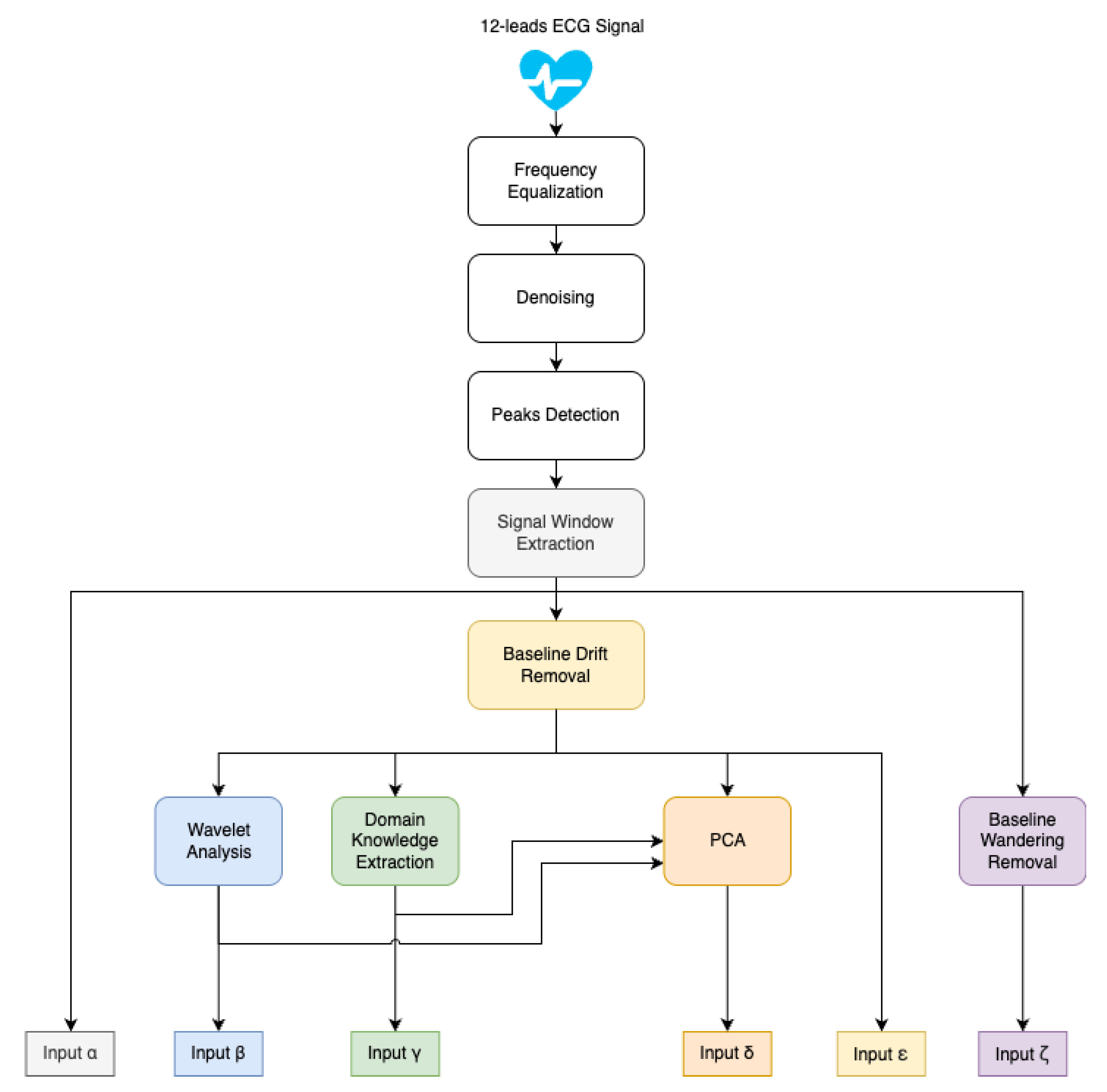
Figure 2.
Scheme of Multibranch network architecture.
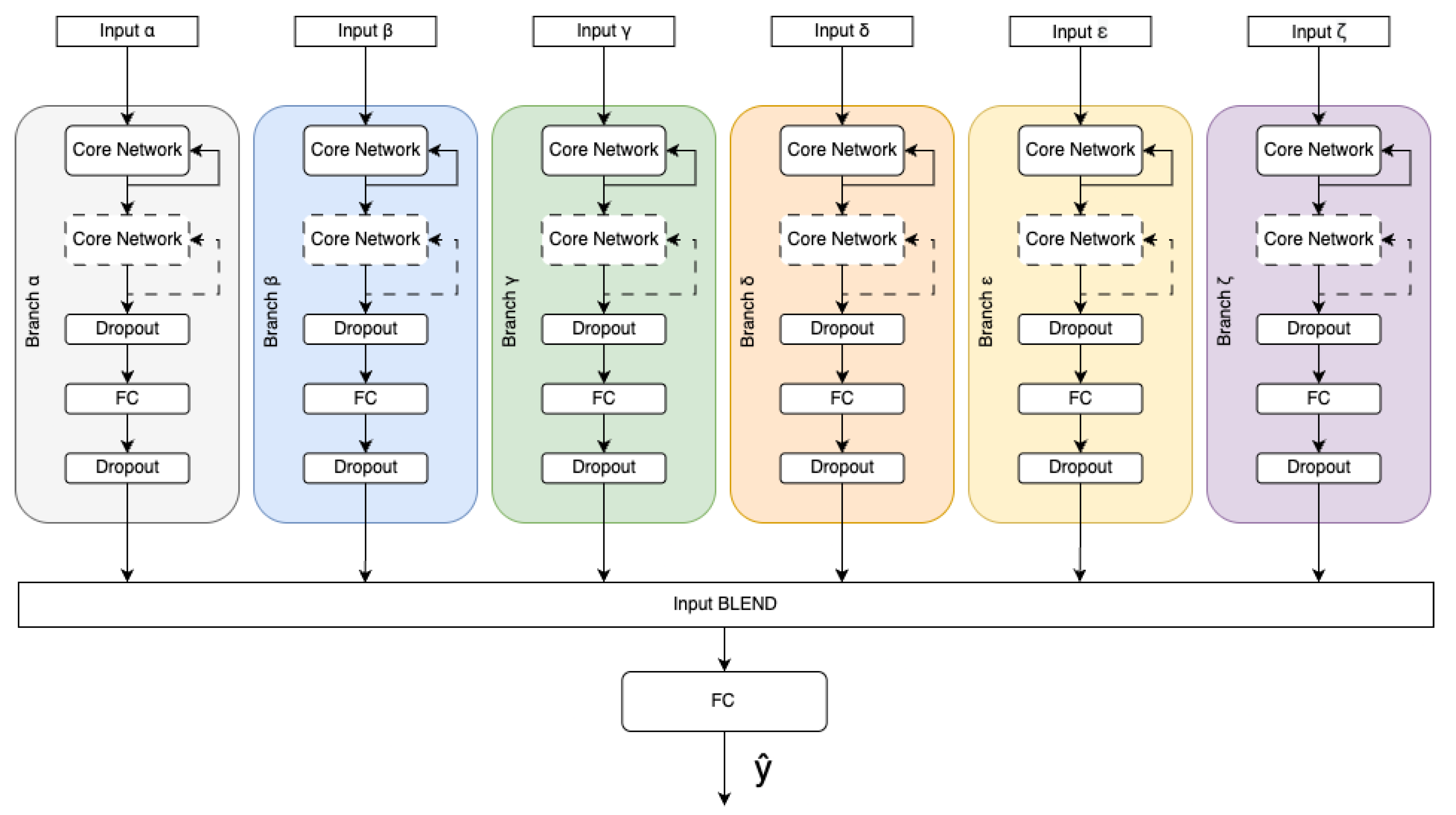
Figure 3.
Construction of feature matrix representing domain knowledge [22].
Figure 3.
Construction of feature matrix representing domain knowledge [22].
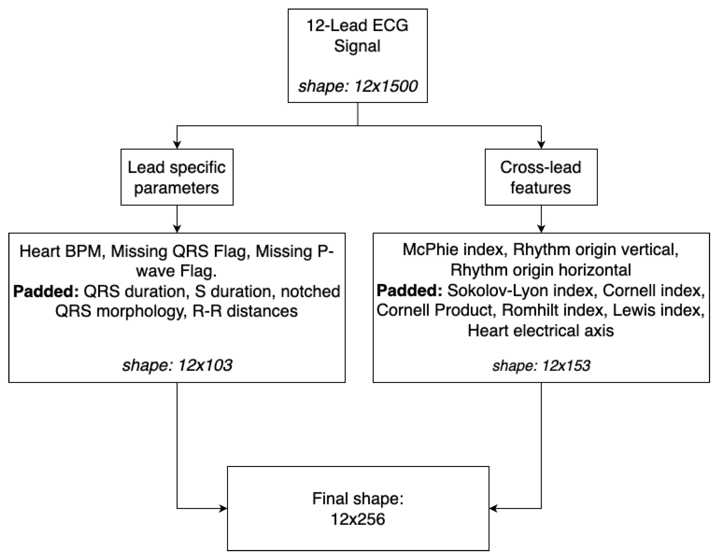

Table 1.
Comparison of used datasets.
| Dataset | Number of samples | Length [s] | Sampling [Hz] |
|---|---|---|---|
| [32] | 10 330 | 6 – 144 | 500 |
| [33] | 74 | 1800 | 257 |
| [34,35] | 22 353 | 10 – 120 | 500 or 1000 |
| [36,37] | 10 344 | 5 – 10 | 500 |
| [38,39] | 45 152 | 10 | 500 |
Table 2.
Scenario A – Comparison of LSTM single-branch architecture for different inputs. Results are averages from tests on 5 folds, time for single window classification is in seconds, avg is the average challenge score, and std is the standard deviation for the challenge score.
Table 2.
Scenario A – Comparison of LSTM single-branch architecture for different inputs. Results are averages from tests on 5 folds, time for single window classification is in seconds, avg is the average challenge score, and std is the standard deviation for the challenge score.
| Branch | Time [ms] | F-measure | AVG | STD |
|---|---|---|---|---|
| 0.075 | 0.196 | 0.319 | 0.015 | |
| 0.070 | 0.221 | 0.337 | 0.020 | |
| 0.073 | 0.156 | 0.269 | 0.005 | |
| 0.092 | 0.174 | 0.285 | 0.032 | |
| 0.074 | 0.204 | 0.327 | 0.005 | |
| 0.082 | 0.183 | 0.296 | 0.016 |
Table 3.
Scenario B – tests possible differences between core network architectures working on different branches. The core network was configured with two hidden layers, with seven neurons each, and a dropout layer. Results are averages from tests on 5 folds, time for single window classification is in milliseconds, avg is the average challenge score, and std is the standard deviation for the challenge score.
| Branch | LSTM | N-BEATS | GRU | |||||||||
| Time | Fm | AVG | STD | Time | Fm | AVG | STD | Time | Fm | AVG | STD | |
| 0.10 | 0.252 | 0.415 | 0.010 | 0.12 | 0.100 | 0.282 | 0.004 | 0.11 | 0.161 | 0.328 | 0.028 | |
| 0.09 | 0.268 | 0.441 | 0.009 | 0.12 | 0.128 | 0.299 | 0.015 | 0.10 | 0.230 | 0.400 | 0.057 | |
| 0.23 | 0.101 | 0.288 | 0.004 | 0.11 | 0.097 | 0.281 | 0.006 | 0.25 | 0.099 | 0.274 | 0.005 | |
| 0.10 | 0.247 | 0.416 | 0.021 | 0.11 | 0.134 | 0.292 | 0.016 | 0.10 | 0.198 | 0.364 | 0.023 | |
Table 4.
Scenario C – Comparison of LSTM, N-BEATS and GRU networks in 6-branch architecture. Results are averages from tests on 5 folds, time for single window classification is in milliseconds, avg is the average challenge score, and std is the standard deviation for the challenge score.
Table 4.
Scenario C – Comparison of LSTM, N-BEATS and GRU networks in 6-branch architecture. Results are averages from tests on 5 folds, time for single window classification is in milliseconds, avg is the average challenge score, and std is the standard deviation for the challenge score.
| Network | Time [ms] | F-measure | AVG | STD |
|---|---|---|---|---|
| LSTM | 0.40 | 0.294 | 0.456 | 0.017 |
| N-BEATS | 0.53 | 0.178 | 0.335 | 0.039 |
| GRU | 0.37 | 0.287 | 0.456 | 0.005 |
Table 5.
Scenario D – Comparison of LSTM, N-BEATS and GRU networks in 6-branch architecture for bigger networks. Results are averages from tests on 5 folds, time for single window classification is in milliseconds, avg is the average challenge score, and std is the standard deviation for the challenge score.
| Network | Time [ms] | F-measure | AVG | STD |
|---|---|---|---|---|
| LSTM | 0.41 | 0.314 | 0.486 | 0.012 |
| N-BEATS | 0.51 | 0.227 | 0.390 | 0.017 |
| GRU | 0.36 | 0.269 | 0.432 | 0.027 |
Table 6.
Scenario E – Results of dropout and prune strategies testing on multi-branch LSTM core network. Results are averages from tests on 5 folds, time for single window classification is in milliseconds, avg is the average challenge score, and std is the standard deviation for the challenge score.
| Dropout | Prune | Time [ms] | F-measure | AVG | STD |
|---|---|---|---|---|---|
| NO | NO | 0.38 | 0.295 | 0.448 | 0.011 |
| YES | NO | 0.40 | 0.302 | 0.465 | 0.011 |
| YES | 5% L1 each epoch | 0.41 | 0.294 | 0.456 | 0.017 |
| YES | 5% Random each epoch | 0.41 | 0.288 | 0.440 | 0.023 |
| YES | 20% L1 Once | 0.40 | 0.301 | 0.465 | 0.011 |
| YES | 20% Random Once | 0.34 | 0.211 | 0.283 | 0.039 |
| YES | Decreasing each 2 epoch from 5% to 1% L1 | 0.43 | 0.296 | 0.459 | 0.009 |
| YES | Decreasing each 3 epoch from 5% to 1% L1 | 0.42 | 0.295 | 0.460 | 0.005 |
Table 7.
Scenario F – tests performance of the multi-branch architecture when 5 out of 6 branches are provided. Results are averages from tests on 5 folds, time for single window classification is in milliseconds, avg is the average challenge score, and std is the standard deviation for the challenge score.
| Inputs | LSTM | |||
| Time | Fm | AVG | STD | |
| all branches | 0.40 | 0.302 | 0.465 | 0.011 |
| removed | 0.38 | 0.289 | 0.456 | 0.012 |
| removed | 0.39 | 0.285 | 0.445 | 0.012 |
| removed | 0.24 | 0.292 | 0.456 | 0.024 |
| removed | 0.37 | 0.291 | 0.453 | 0.033 |
| removed | 0.36 | 0.285 | 0.444 | 0.037 |
| removed | 0.36 | 0.289 | 0.455 | 0.029 |
Table 8.
Scenario G – Comparison of LSTM, N-BEATS and GRU networks in 6-branch architecture for bigger networks with different prune strategies. All tests used a dropout layer. Results are averages from tests on 5 folds, time for single window classification is in milliseconds, avg is the average challenge score, and std is the standard deviation for the challenge score.
| Network | Pruning strategy | Time [ms] | F-measure | AVG | STD |
|---|---|---|---|---|---|
| LSTM | 5% L1 each epoch | 0.41 | 0.314 | 0.486 | 0.012 |
| No prune | 0.40 | 0.318 | 0.477 | 0.013 | |
| 20% L1 once | 0.67 | 0.318 | 0.477 | 0.013 | |
| N-BEATS | 5% L1 each epoch | 0.51 | 0.227 | 0.390 | 0.017 |
| No prune | 0.49 | 0.225 | 0.386 | 0.022 | |
| 20% L1 once | 0.50 | 0.225 | 0.386 | 0.022 | |
| GRU | 5% L1 each epoch | 0.36 | 0.269 | 0.432 | 0.027 |
| No prune | 0.38 | 0.261 | 0.429 | 0.033 | |
| 20% L1 once | 0.63 | 0.261 | 0.429 | 0.017 |
Table 9.
Comparison of state-of-the-art solutions for CinC 2021 Challenge dataset on 12-lead ECG classification with proposed solution. First five places were obtained by different CNN variants.
Table 9.
Comparison of state-of-the-art solutions for CinC 2021 Challenge dataset on 12-lead ECG classification with proposed solution. First five places were obtained by different CNN variants.
| Network | Paper | Challenge score |
| ResNet (CNN) | [42] | 0.58 |
| WRN (CNN) | [43] | 0.55 |
| 2-branch CNN | [44] | 0.55 |
| Channel-Attention CNN | [45] | 0.55 |
| ResNet (CNN) | [46] | 0.52 |
| Multibranch LSTM (RNN) | (this paper) | 0.49 |
| Bidirectional LSTM (RNN) | [47] | 0.36 |
Disclaimer/Publisher’s Note: The statements, opinions and data contained in all publications are solely those of the individual author(s) and contributor(s) and not of MDPI and/or the editor(s). MDPI and/or the editor(s) disclaim responsibility for any injury to people or property resulting from any ideas, methods, instructions or products referred to in the content. |
© 2025 by the authors. Licensee MDPI, Basel, Switzerland. This article is an open access article distributed under the terms and conditions of the Creative Commons Attribution (CC BY) license (http://creativecommons.org/licenses/by/4.0/).
Copyright: This open access article is published under a Creative Commons CC BY 4.0 license, which permit the free download, distribution, and reuse, provided that the author and preprint are cited in any reuse.


