
Submitted:
04 March 2025
Posted:
05 March 2025
You are already at the latest version
Abstract
The biology literature addresses two puzzles: i) the increase in specific metabolic rate of organs (SOrMR, W/kg of organ) with a decrease in body mass (MB) of biological species (BS), and ii) how the organs recognize they are in a smaller or larger body and adjust metabolic rates of the body ( ) accordingly. These puzzles were answered in the author’s earlier work by linking the field of oxygen-deficient combustion (ODC) of fuel-particle clouds (FC) in engineering to the field of oxygen-deficient metabolism (ODM) of cell clouds (CC) in biology. The current work extends the ODM hypothesis to predict the whole body metabolic rates of 114 BS and demonstrates Kleiber’s power law { }. The methodology involves the i) extension of the effectiveness factor relation, expressed in terms of the dimensionless group number G (= Thiele Modulus2), from engineering to the organs of BS, ii) modification of G as GOD for the biology literature as a measure of oxygen deficiency (OD), iii) collection of data on organ and body masses of 116 species and prediction of SOrMRk of organ k of 114 BS using only the SorMRk of two reference species (Shrew, 0.0076 kg: RS-1; Rat, 0.380 kg: RS-2), iv) estimation of of 114 species versus MB and demonstration of Kleiber’s law with a = 2.962, b = 0.747, and v) extension of ODM to predict the allometric law for maximal metabolic rate (MMR under exercise, { }.) and validate the approach for MMR by comparing bMMR with the literature data.
Keywords:
Metabolism
; Kleiber’s Law
; Oxygen Deficiency
; Maximum Metabolic Rate
; Organ-GOD Number
1. Introduction, Literature Review and Objectives
Recent efforts aim to connect thermodynamics and combustion with biology to better understand the virus evolution, develop empirical formulae for viruses, and analyze biological processes through Gibbs function and energy release within biological systems (BS) [1,2,3]. This study extends previous work linking the field of oxygen-deficient combustion (ODC) with oxygen-deficient metabolism (ODM) [3] to predict the specific organ metabolic rates (SorMRk) of vital organ k of mass mk (W/kg of k, k= Kidneys (Kids), Heart, Brain and Liver) of 114 BS ranging in mass from 10 g to 6,650 kg by using i) data on SorMRk of two BS named as reference species (Shrew, 0.0076 kg: RS-1; Rat, 0.390 kg: RS-2), ii) data on organ masses of 116 species (114 +2 RS), and iii) established metabolic energy release relationships from ODC/porous char combustion literature. By summing the organ metabolic rates {MR} of individual organs (OrMRk=SorMRk x mk) across all organs, the whole-body metabolic rate (BMR) as a function of body mass (MB) is obtained. The ODM approach is validated by demonstrating Kleiber’s law and comparing the predicted allometric constants with literature data. The study provides a brief overview of Kleiber’s law, followed by i) a review of current theories explaining the ¾-power law, ii) an introduction to ODC, the dimensionless group number G , ODM and corresponding GOD # for organs, iv) the methodology adopted for the prediction of SOrMRk of 114 species using only two RS, and v) validation and extension to allometry for maximal metabolic rate (MMR). A higher GOD # indicates a higher degree of oxygen deficiency.
1.1. Kleiber’s Law and Organ Metabolic Rates
Allometry refers to how the characteristics of biological species (BS), including morphological traits (e.g., brain size) and physiological traits (e.g., metabolic rate (MR), life span), change with body mass. The allometric relation for MR in BS is given as:
where MB is body mass
(kg) and (), MR is in watts. In 1932, Kleiber obtained a = 3.4, b = 0.74 for MB ranging from 0.15 to 679 kg, known as Kleiber’s law [4,5], which persisted for over 70 years [6]. The specific basal metabolic rate (SBMR, W/kg of body mass) is written as
Where b’ = b - 1 = -0.26
Nutrients consumed through the mouth are essential for energy release through oxidation. The review in Ref. [[8] suggests that O2, which enters through nasal intake, must also be considered a “nutrient” since it is essential for energy release. The energy release rate (ERR) is related to the oxygen consumption rate within whole body since ERRB = , where HHVO2 t is the energy release per unit mass of oxygen consumed and it is almost constant at about 14335 J/g of O2 for most fuels and nutrients [1]. If O2 supply falls below a critical level then its uptake is limited by the supply from blood vessels, which is a common assumption used in the classical WBE {West, Brown and Enquist} hypothesis for demonstrating Kleiber’s law.
The scaling function for metabolic rate with body size MB is explained with two existing theories:
I). West et al. [7] proposed a fractal or “nutrient (including oxygen) distribution network” hypothesis (also referred to as the “upstream” or supply side [8] or “outward-directed vascular network” [9]) and illustrated Kleiber’s law by minimizing the heart’s work required to pump the unit amount of blood, i.e., a network which minimizes the pressure difference (Paorta-Pcap). The scaling function is explained with O2 delivery to cells as the limiting factor.
II). Bejan [10,11] proposed that architectures and organs must develop in such a way that resistance to flow current (e.g., water flow in trees) must be minimized, or equivalently, that entropy generation is minimized, resulting in lower energy consumption and food requirements.
The Biologists have raised the following issues as unknown: “The allometric size relationship is somehow ‘programmed’ into cells, although the factors that let them know whether they are in a small or large organism are still unknown” [12]. That is, existing biological data indicates that organs increase their metabolic rates per unit mass when within a smaller body and vice versa. In earlier work, the author proposed the “Oxygen-Deficient Metabolism (ODM)“ hypothesis to explain these unknowns [3]. In the current work the same ODM hypothesis is extended to predict the specific organ metabolic rate of organ k {SOrMRk , k= k= kidneys (kids), heart, brain and liver} of 114 BS ranging in mass from 10 g to 6,650 kg using data on SOrMRk of two reference BS { RS-1 of lowest MB , Shrew, 7.5 g; RS-2 elected with MB much higher than that of RS-1: Rat, 380 g }. With known vital organ masses mk , the OrMRk {= SOrMRk · mk} are estimated and summed up to yield the whole-body basal metabolic rate as a function of body mass (MB) for 116 BS ranging in mass from 0.0076 kg to 650 kg, The log-log plot yields Kleiber’s law for 116 species ranging in mass from 0.007 kg to 650 kg, with an allometric exponent of b= 0.747. More importantly, the ODM presents a dimensionless group (GOD)k for biology literature to indicate the extent of OD within an organ.
1.2. Literature Review
While combustion is a rapid oxidation process that typically occurs at high oxygen mass fraction, YO2,air = 0.23 (mole fraction =0.21 or 23% or 210,000 ppm), resulting in a significant temperature rise, the metabolism is a slow oxidation process that typically occurs at a low oxygen mass fraction, YO2 ( [13]), where pO2 is the partial pressure of O2 in mm of Hg. While the pO2 in alveolar is 106 mm of Hg , the pO2 in tissues is about 40-50 mm Hg and dissolved O2 is on the order of 1-6 ppm, thus resulting in a lower temperature rise. Sometimes, the biology literature calls as “heat produced” or “power produced“ [51], while the engineering literature defines as the energy release rate (ERR) by all the cells within the body. The is a sum of the work delivery rate, , (i.e., ATP delivery rate, approximately 25% of ) and the heat transfer rate (, approximately 75 % of , [52]) due to the temperature difference (ΔT) across the cells and the rest of the body.
The required O2 uptake (biology uses volume units in mL/min, in mg/min=1.42 x ) by mitochondria in the cells is supplied by blood vessels via capillaries, followed by diffusion from capillaries to cells and then from cells to mitochondria.
The hypotheses used for demonstrating Kleiber’s law { vs MB } fall under two broad groups: I) Homogeneous and II) Heterogeneous.
I). Homogeneous hypothesis:
This hypothesis considers the whole body as a system; the hypotheses include: i) the law of surface area to volume ratio of the whole body, yielding b=2/3, b’=-1/3, as described by Rubner’s law in 1883, ii) WBE’s fractal geometry [14] (geometry of circulatory system: macro and microcirculation), which relies on minimization of dissipative energy in the vascular system supplying oxygen and nutrients. Savage et al. showed that the WBE model is applicable only for BS of infinite body size (or network) [15], and when finite size is included, it yields scaling exponents as a function of body size. Further, Weibel and [16] question the universal models based on “the fractal design of the vasculature and the fractal nature of the total effective surface of mitochondria and capillaries” since they predict b= ¾ for both basal and maximal metabolic rates. Silva et al. [17] suggest that there are mathematical and conceptual errors in network models, weakening the proposed theoretical arguments. The same review suggests that the power law exponent b should vary between 2/3 and 1 based on ‘metabolic level’ (activity level of the organism or metabolic intensity). Painter et al. [18] agreed with the assumption of blood volume ∝ MB but questioned the assumptions of uptake nutrient consumption rate (called total current in the network) proportional to blood volume, iii) network structures [9], iv) quantum mechanics [19], and v) topology [10].
II). Heterogeneous Hypothesis:
The heterogeneous hypothesis considers the whole-body metabolic rate as a sum of the OrMRk with k= kids, H,Br,L and RM where RM represents all the remaining weakly metabolizing tissues. The mass of RM is given as
a) Body Mass Based Allometry Wang et al. used a heterogeneous or reductionist approach for estimating the whole-body metabolic rate { } [20,21,22]:
where is the SOrMRk of kth organ { W/kg of k}given by the body mass based allometry (BMA) given by
Here afterwards, this method of computing SOrMRk using the empirical allometric relations ( EAR) will be termed as EAR method. Wang et al. presented allometric relations for organ masses [21]:
Using Equation 4 and Equation 5 , the is obtained as
Based on data on the organ mass and of six species (ranging from 0.48 kg of rat to 70 kg of human), Ref. [21] tabulates the constants ck,6, dk,6, ek,6 and fk,6. Table 1 tabulates the allometric constants ck,6, dk,6, ek,6 and fk,6. Since dk,6 6 > 0, organ sizes are positively related to MB, while the SOrMRk, Equation 4) are negatively correlated with body mass (fk,6<0). The additional subscript “6” indicates that the empirical constants are based on six species. As opposed to a majority of BS, , human brain masses are relatively larger, and the allometric relation underpredicts mBr for humans. Thus, human brain mass is estimated using the encephalization quotient (EQ), which is the ratio of measured brain mass to the mass predicted with allometry. Gallagher et al. report that for a reference human of 70 kg [23], the RM for the 5-organ model is 66.2 kg, while the masses of Kids, H, Br, and L are 0.31, 0.33, 1.4 and 1.8 kg, respectively; this results in 94.5% of body mass being RM, while vital organs account for 5.5%. Each of these vital organs contribute 8.7% (Kids), 8.2% (Heart), 21.6% (Brain) and 20.2% (Liver) of the total BMR [24]. However, if one uses the data on ck,6 and dk,6 tabulated in Table 1, the resulting mass percentages are 0.37% (Kids), 0.58% (Heart), 0.40% (Brains) and 1.90% (Liver), with vital organ mass percentage at 3.25%. The corresponding energy percentages are 7.36% (Kids), 12.81% (Heart), 3.97% (Brain), and 17.10% (Liver), with vital organ energy percentage at 41%. While the brain mass for 70 kg human is predicted as 0.28 kg from allometry, Gallagher’s data brain mass is 1.4 kg indicating high EQ. The underprediction of human brain mass and energy percentage is due to the EQ factor, as humans have the highest EQ (i.e., a larger brain size compared to animals of similar mass). This additional brain mass enhances cognitive abilities beyond general brain mass versus body mass scaling laws. See Section 3.4 for further discussion on brain mass and its effects on human results.
b) Organ Mass Based Allometry (OMA) Exponents for SOrMRk or : It is noted that “fk,6” in BMA for the vital organs of the six species selected in EAR by Wang et al. [21] are all negative. To explain the negative values of fk,6 in BMA for organs, the BMA is replaced by organ mass-based allometry [3], using the relation between organ mass and body mass. Thus,
where
See Table 1 for the listing of Ek,6 and Fk,6. The Fk,6 becomes more and more negative for increasing organ masses. Ref. [3] explains the rationale for Fk,6 vs mk using the ODM hypothesis. It is apparent from the constant ek,6 and f k,6, or Ek,6 and Fk,6 (Table 1) that different organs consume oxygen at different rates, thus indicating different O2 profiles. Since the ODM hypothesis is used to predict SOrMRk and demonstrate Kleiber’s law in the current work, a brief outline of Ref. [3] on ODC and ODM is presented below for the convenience of readers.
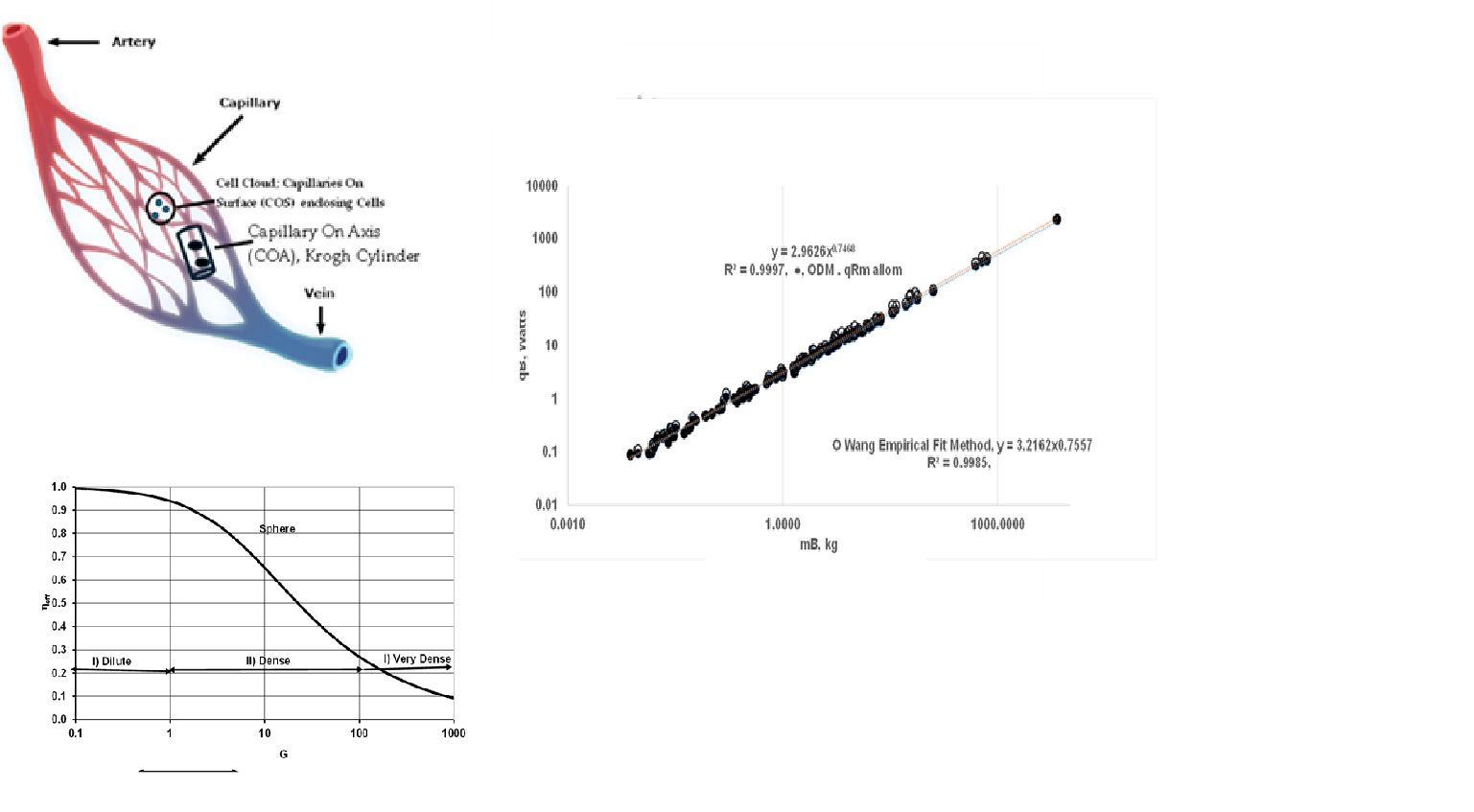
B) Group or Oxygen-Deficient Combustion (GC or ODC) in Engineering: The engineering literature models the combustion of dense fuel particle suspension (e.g., coal suspensions fired into a boiler) using a spherical fuel-particle cloud of radius R,FC , mass mFC and number density of fuel articles nFC, with its surface exposed to a known oxygen mass fraction at the surface YO2,FC,s (Figure 1) where FC stands for fuel cloud. Thus, the oxygen concentration, YO2(r), within the FC is a function of r, and consequently, the energy release rate (ERR) varies as a function of r, with the highest value near aerobic cloud surface and lowest value at the core of the suspension. This model is referred to as a group combustion or oxygen-deficient combustion (GC or ODC) in engineering literature, implying that particles at the core may not receive enough oxygen to burn. Detailed literature on ODC in engineering is provided in a three-part series of articles [25,26,27]. The local O2 consumption rate by each particle located at r { }, is given as (Figure 1d)
where the characteristic oxygen consumption rate, Cch,p, for each particle changes depending on kinetics control (CCh,p = CCh,p,kin) with a first-order reaction or diffusion control (CCh,p = CCh,p,dif ). The basic relations for Cch,p are given in Ref. [3]. The engineering literature presents the solutions for the i) YO2(r) profiles within the fuel cloud (FC) and ii) the consumption rate of O2 by all the particles within the cloud . The energy release rate (ERR) of FC is given in terms of oxygen consumption by FC {, See Table 1 for HHVO2 }. Then, the specific energy release rate of whole cloud , SERRm, is given as ERR/mFC. The SERRm decreases with an increase in R,FC or m,FC – that is, the increase in ERR is less than proportional to the increase in m,FC due to core particles contributing negligible energy release due to OD. The solutions for , or ERR of FC, are presented in terms of the effectiveness factor (ηeff,,FC) of the FC. The ηeff,,FC is defined as a ratio of the O2 consumption rate by all particles within the cloud to the rate of consumption of O2 in the case that each particle within the FC is subjected to YO2,FC,s.
The solution for ηeff,FC for a spherical FC is obtained with known YO2(r) profiles:
where the dimensionless group G for FC is defined as:
and the G number for FC is shown to be related to Thiele Modulus, ΨT (G= ΨT 2) in porous char combustion literature [26,27,28]: Using Equation 10, the effectiveness factor can be plotted against G as shown in Figure 2. It is noted that G ∝ RFC 2, and since the mass of the fuel cloud, mFC ∝ RFC 3 and hence G ∝ mFC (2/3), assuming a constant number density of fuel particles (nFC).
Figure 2 shows the results for ηeff vs. G for a spherical FC. There are three regimes of FC oxidation: Zone I – Dilute Cloud {G<1} where a low number density “nFC” for given FC size RFC or smaller cloud size for given number density “nFC” i.e. “mFC” low) a) indicates high SERR (W/kg). It is constant throughout the cloud since YO2 = YO2,FC, s and ηeff,FC ≈ 1. The particles in Zone I burn almost uniformly with an O2 concentration at YO2,FC, s for all particles as though each particle is isolated. Zone II – Dense Cloud {1 < G < 100} , where the cloud size RFC is large, “mFC” is higher, and SERR is a function of r since YO2 (r) < YO2,FC, s. This is the ODC mode or “crowd” effect as called in biology [12], where oxygen concentration decreases with decreasing r, forming an anaerobic core of radius Ran where the O2 concentration is almost zero. For this zone, ηeff,FC < 1 (Figure 1b). Zone III – Very Dense Cloud {G > 100}, where particles at the core experience severe ODC, with G > 100. (Figure 1c). Except for a thin aerobic film near the surface of FC, the anaerobic core radius is almost the same as RFC. For this zone, ηeff,FC << 1.
C) Oxygen-Deficient Metabolism (ODM) in Biology:
The oxygen diffuses from capillaries towards the metabolic cells contained within interstitial fluid (IF). Even though the biology literature suggests a radial diffusion distance of the order of 100 μm (where pO2 ≈ 0) from the capillaries, the actual path may be longer, leading to a decreased O2 transport rate (or decreased effective diffusivity) to the mitochondria. The diffusive O2 transport rate is affected due to the following:
If the mass of each kidney (k= Skid, single kidney) is used, mSkid = mKid/2, HHVO2= 14,335 kJ/kg of O2 or 18.7 kJ/SATP L of O2 or 20.5 J/CST mL of O2 or 18.1 J/mL of O2 at 36.2 °C
HHVO2, kJ/L O2 71 to 92 kg = 15.818 + 5.17* RQ [30,31,32]: i) closely packed cells (number density of cells, n, or crowding effect) [33], ii) tortuous oxygen path, iii) amount of aqueous fluid, iv) extracellular structures or cell barriers, and v) presence of cytoplasm (which alone reduces D by 30 times the normal level). As a result, cells cannot maintain the required O2 flow for ATP production [34], leading to oxygen deficiency (OD).
ODM in Organs: Hypoxic conditions (low pO2 in cells) decrease the oxygen consumption rate by cells, while anemic conditions or a reduction in blood flow [35] or reduced Hb contents cause a decrease in O2 supply to the cells from capillaries. Hypoxic conditions cause in reduction of ATP production rate leading to “bioenergetic collapse” [36]. Furthermore, YO2 within cells may fall below the “extinction” level, causing cells to cease oxidation and become sleeper cells. OD in cells under hypoxic conditions prevent oxidation of pyruvate and hence it converts to lactate, increasing acidity which then results in the production of protein called HIF (hypoxia-induced factor). HIF enables the activity of genes to switch from oxidative phosphorylation to glycolytic pathways [37] for energy and ATP release, altering the apparent “software” for energy release from oxidation to glycolysis. ODM promotes a switch to glycolysis, where only two ATP are obtained per CH compared to 32 ATP via oxidative phosphorylation, resulting in the decrease of overall energy release [38] via glycolysis path. Increased ATP requirements cause consumption of more nutrients to adopt an altered metabolic path for energy release, i.e., glycolysis under low-oxygen environments, which supports rapid cell division and serves as a source of energy for cancer cells [39,40]. Rats are known to sustain anoxia for extended periods by using fructose as a nutrient for glycolysis [13,41]. It is well known that oxygen deficiency (OD) or hypoxia contributes to several diseases, including cancer, stroke, anemia and heart disease. There appears to be a positive correlation between the mass of an organ and the number of cancer cases [42], which is attributed to the link between excess fat in organs and obesity.
ODM in Cell Clouds:
Singer’s Phenomenological type of ODM Model: Singer et al. studied the role of OD or the “crowding effect” on the metabolic rates of in-vitro organ samples and developed a phenomenological type of model. Just like particles in FC, the cells near the aerobic surface undergo high SOrMRk while those cells near the anerobic core may undergo only glycolysis.
Detailed ODM Model following ODC Literature in Engineering: More detailed ODM models were developed by Annamalai by adapting the ODC literature from engineering to biology [3]. Unlike the Krogh cylinder model, where the capillary is placed on the axis (COA) of a cylinder containing metabolic cells , the ODM model uses a spherical cloud of cells (CC) of radius RCC having nCC, cells per unit volume with capillaries on the surface (COS) of CC with mass of CC, mcc {Figure 3a}. The COS model is also known as the “solid cylinder” model in biology [43]. A detailed comparison between ODC and ODM models, and relations for several variables of interest, are presented in Ref. [3]. In ODM, the carbon cloud is replaced by a cell cloud (CC), particles are replaced by cells of the BS, and YO2,FC,s becomes YO2,CC,s. The radius RFC is replaced by RCC, the ERR is replaced by the organ metabolic rate (OrMR) and ERRm is replaced by SOrMR in cell clouds, defined as SOrMR = OrMR / mCC. The G number in engineering ( [27]) is also replaced by GOD,k for organ k. The oxidation rate for each particle is replaced by the cell metabolic rate (Figure 3d). These relations will be summarized in the methodology section.
Just like FC, there exists three zones of operation of CC: Dilute, Dense and very dense CC. More details for CC are provided in the caption of Figure 2. Those cells near the surface are aerobic with higher rate of oxidation of nutrients while those cells near the core of the cloud are anaerobic with very little oxygen. Cells near core may undergo only glycolysis {Figure 3b}.
While resting, limited capillaries are perfused with blood (Figure 3b, surface at YO22,cc,s), whereas under exercise, all the capillaries are perfused (Figure 3c} increasing YO22,CC,s at the surface of CC { e.g., Maximum Metabolic Rate (MMR) when there is increased blood flow through selected organs during exercise}.
The literature review suggests that despite several hypotheses outlined in Section 1.2 for the 3/4 law, “the hunt for an explanation of the 3/4 law continues” [44]. The current ODM hypothesis focusses on the metabolic rate he controlled by “downstream demand-side” oxygen consumption of all the cells within an organ and provides another “hunt” for an explanation of the 3/4 law. Attempts have also the been made to extend ODM hypothesis predict the allometric constants of maximal metabolic rate (MMR) vs. body mass using known data on the percentage of blood perfused under rest and during exercise, attributing the increase in MR to enhanced oxygen concentration under the redistribution of perfusion percentage of capillaries.
1.3. Objectives
The overall objectives of the current work are to i) link the field of group or oxygen-deficient combustion (ODC) in engineering with the field of oxygen-deficient metabolism (ODM) in biology, ii) adopt the relations developed for energy release rate per unit mass (ERRm, W/kg cloud) to predict SOrMRk (W/kg of k) of 116 BS ranging in mass from 0.0075 to 6,650 kg using known data from two BS, referred to as Reference Species (RS), where RS-1 has the lowest body mass, MB,RS-1 (Shrew, 0.0075 kg), and RS-2 has mRS-2 body mass much higher than mRS-1 (Rat Wistar of 0.390 kg, ηeff,k < 1), and iii) estimate the whole-body metabolic rate versus MB using a heterogeneous approach and known organ masses, demonstrating Kleiber’s law with an exponent close to 0.75. In addition, predict a) a hypothetical upper metabolic rate (UMR) for organs, and, consequently, the whole body in the case all the cells within the organ metabolize without the presence of oxygen concentration gradients, b) the maximal metabolic rate (MMR) under exercise, when all the capillaries at the cell cloud surface are perfused, with increased average oxygen concentration at the cell cloud surface (CC,s) and show that whole-body allometric law yields an exponent close to 0.87, as quoted in the literature, and c) provide a method for detecting the degree of oxygen deficiency within organs for medical personnel.
2. Materials and Methods
2.1. ODM Hypothesis
The ODM hypothesis assumes that each organ k consists of multiple cell clouds (CC), with each cell cloud having a mass mass mcc,k with radius RCC,k, which is related to the organ mass mk by RCC,k α mk 1/3. It is also possible that capillaries do not fully cover the entire spherical surface enclosing the cells (Figure 3). Typically, 25-35 % of an organ’s capillaries are perfused at rest, with perfusion increasing during exercise since there is increased metabolic demand and a higher perfusion percentage results in a higher YO2,cc,s. Using the Krogh-Erlang equation, Ostergaad demonstrated that only 10% of SM capillaries are perfused at rest, but more capillaries are recruited during exercise [46]. Further details can be found in Section 2.2 and Section 3.4.
Smaller species have smaller organs (e.g., shrew of mass 0.0075 kg), while larger species have larger organs, as indicated by dk > 0 in the allometric exponents for organ sizes. Thus, the smaller organs of smaller species may have shorter distances for O2 diffusion from capillaries to cells, allowing metabolism to occur as if each cell within the CC is exposed to the same O2 concentration as YO2,CC,s (ηeff ≈1), resulting in SOrMRk ≈ SOrMRk,iso,. However, isolated cell metabolic rates can still vary from organ to organ, even in smaller species, due to differences in functional requirements, cell reactivity, and O2 transport rate (e.g., heart tissues containing Mb can deliver O2 at faster rate resulting in increased effective transport coefficients for O2 from capillaries to mitochondria). As organ mass increases (e.g., in the liver), ηeff,k < 1, and SOrMRk ≈ ηeff,k x SOrMRk,iso, where it is assumed that for any given organ k, SOrMRk,iso remains constant for all BS regardless of body size, but becomes extremely low for larger organs in larger species, leading to lower values of ηeff,k.
2.2. Methodology
Detailed comparisons of the governing conservation equations and several relations in the fields of ODC in engineering and ODM in biology literatures are presented in Ref. [3]. These include: i) conservation equations for both fields, ii) the ERR of a single particle in a FC and a single cell in a CC in terms of YO2, iii) oxygen profiles in FC versus CC, iv) the dimensionless G number for FC {Equation 118 } and corresponding GOD,k for the CC of organ k in biology { Equation 14} and v) the specific ERR (SERR) of FC (W/kg of cloud) in terms of the effectiveness factor and G, and specific organ metabolic rate (SOrMRk) of CC (W/kg of cell cloud of organ k) in terms of the effectiveness factor and GOD, k. The relevant relations for the current work are briefly summarized below.
- i)
- Metabolic Rate of single cell located at r in CC {Figure 3}
where CCh,cell, characteristic cell O2 consumption rate when YO2 = 1; the relations for CCh,cell under kinetic control or diffusion controlled O2 consumption rates are given in Ref. [3].
- ii)
- Oxygen Profiles within CC
For the cell cloud within organ k, Ref. [3] presents
where for organ k
where k= Kid, H, Br, L and RCC,k α mk1/3, CCh,cell, characteristic O2 consumption rate by cell
- iii)
- Effectiveness Factor of Spherical CC and Specific Organ Metabolic Rate {SOrMRk}
Adopting the same procedure as in engineering,
With YO2 profile from Equation 13, the ηeff,k is derived as:
where k = Kids, H, Br, and L Using the definition of ηeff,k , the SOrMRk is given as
where . Equation 17 reveals that SOrMRk is a function of GOD,k in biology due to dependence of ηeff,k on GOD,k . I) When GOD,k << 1 (dilute cloud), then, ηeff,k→1 (Equation 1613, Figure 2 with ηeff = ηeff,k, G = GOD,k). II) As the organ size increases, GOD,k also increases, and the effectiveness factor decreases (dense cloud, 1 < GOD,k < 100). III) When GOD,k > 100, the cell cloud is very dense. All three regimes of ηeff,k of CC within an organ are shown in Figure 2.
- iv)
- Metabolic Rate of Vital Organs {}: Using Equation 17 for the vital organs, the metabolic rates of vital organs of any BS:
- v)
- Metabolic Rate of Remaining Mass (RM) of Tissues {} for any BS
The remaining mass of organs (RM) represents a sum of all “minor” organs (e.g., SM, skin, etc.) within the body, and the specific metabolic rate of RM (W/kg of RM) is needed. There are several possible approaches: a) Select data for each of minor organ if available, estimate the effectiveness factor for all minor organs, and adopt a similar procedure outlined for vital organs , b) Use the EAR for RM: , eRM,6 =1.45, fRM,6 = -0.17, in W/kg, c) Assume Elia’s constant values for as 0.581 W/kg for all BS. In the current work, methods (b) and (c) are adopted for estimating .
- vi)
- Whole Body Metabolic Rate () under Rest
The effective area for O2 exchange.is limited, as only 25% to 35% of available capillaries are perfused under BMR conditions [45], which affects O2 diffusion distance and hence the metabolic rate within the organ. Adopting the heterogeneous method, whole body metabolic rate under rest, {} is given as
- vii)
- Metabolic Rate of RM {} and Whole Body Metabolic Rate {} under Exercise
During exercise, blood flow to the skeletal muscle (SM) is increased to supply the required oxygen and nutrients. Thus, SM becomes metabolically more active compared to other tissues within the RM due to increased capillary perfusion, increasing from approximately 25% at rest to nearly 90 % during exercise.
Relations for depends upon the YO2, CC,s and hence the percentage of capillaries perfused. The remaining mass of tissues under exercise is given as
Where is different from under rest due to the percentage of capillaries perfused under exercise are different from those at rest. The during exercise is given as,
- viii)
- Upper Metabolic Rate (UPR,) and Maximum Metabolic Rate (MMR,) of Whole Body
A hypothetical upper MR of organ k (not the maximum MR) and, hence, the whole-body MR can be estimated by setting ηeff,k = 1 for all organs {i.e. no oxygen gradients within CC}, including RM from Equation 1613 to Equation 2016.
When the CC surface is covered with more perfused capillaries, the YO2,CC,s increases and most of the cells are aerobic resulting in the maximum metabolic rate, MMR and leading to a whole-body allometric law with an exponent higher than 0.75. The MMR, such as during exercise, is obtained by setting ηeff,k = 1 for all organs, including SM, and RM-Ex during exercise, while adjusting the percentage of capillaries perfused. Further blood flow to organs other than SM are also altered. This adjustment affects YO2,CC,s for all organs due to change in blood flow rates . The percentage of perfusion affects YO2,CC,s (Figure 3b and Figure 3c). The change in YO2,CC,s is given by the following relation:
The increased YO2,CC,s causes isolated rates to increase, thereby increasing the whole-body metabolic rate. The percentage of capillaries perfused under rest and exercise conditions is shown in . Note that blood flow rate to organ k is given by the product of blood flow fraction to organ k and the pumping rate of blood by the heart and pumping rate changes depending upon the rest or exercise conditions.
2.3. Estimation of OD Number (GOD,k) and Effectiveness Factor (ηeff,k) of Organ k any BS
The estimation of ηeff,k requires knowledge of the dimensionless number GOD,k (Equation 14), which depends on i) the reactivity of cells within organ k undergoing metabolism (CCh,cell) either under diffusion or kinetic control { Michaelis Menten (MM) constant for first order reaction under adsorption control} ii) the overall transport coefficient D of oxygen from capillaries to mitochondria, and iii) a knowledge of (YO2,CC,s)k dictated by capillary number density and percentage of capillaries perfused. There are two methods for estimating SOrMRk of organs:
A) Basic Method: This approach requires basic data for CCh,cell, D, (YO2,CC,s)k, MM constant and the percentage of capillaries perfused for each organ k. Consequently, greater uncertainty exists in the estimation of GOD,k and SOrMRk due to variations in these parameters across the organs of 116 species.
B) Ratio Method or Reference Species (RS) Method:
The current work uses the references species (RS) method, also known as the ratio method, and assumes that the SOrMRk of two references species, RS-1 and RS-2, are known. This approach reduces uncertainty in the results by relying on ratios. This method is based on the premise thats of any BS is same as of RS-1 having lowest body mass and hence lowest organ mass. In RS-1, all cells within the vital organ k operate under an isolated mode (i.e., all cells at YO2,CC,s, ηeff,k ≈ 1). The RS-1 is selected as the BS with the lowest body mass (e.g., RS-1: Shrew, 7.6 g). Justification is as follows. Makarieva et al. [47] demonstrated that SBMR varied from 0.3 W/kg to 9 W/kg (a 25-fold variation), despite a 1020-fold difference in body mass for “bacteria to elephants and algae to trees.” This suggests that SBMR is relatively consistent among mammalian species [48]. Since the number of cells per unit mass is similar across BS, then cell metabolic rate (CMR) does not vary significantly. This view is confirmed by Lindstedt and Schafeer [49], who stated that the “150-ton blue whale,” which is 75 million times the mass of the 2g Etruscan shrew, “shares the same architecture… organ systems, biochemical pathways.” Therefore, the isolated metabolic rate of cells in a vital organ k of any BS is assumed to be same as that of organ k of RS-1.
The RS-2 is selected as a BS with a significantly higher body mass (e.g., Rat Wistar, 390 g) than RS-1. In RS-2, the GOD,k falls within the dense zone (i.e., the steeper part of ηeff,k vs. GOD,k, Zone II in Figure 2), and hence (ηeff,k)RS-2 < 1. With the known SOrMk data for RS-1 and RS-2, (ηeff,k) RS-2 is estimated as
and the corresponding (GOD,k)RS-2 is evaluated using Equation 1613. With the assumption of a constant cell diameter (2a) for a given organ k across BS (Schmidt-Nielsen [58], Savage et al. [49]) and the number density of cells, and using the definition of GOD,k (Equation 14), GOD,k ∝ RCC,k 2 and since the mass of the cell cloud, mCC,k ∝ RCC,k 1/3, GOD,k ∝ mCC,k 2/3, the GOD,k for 116 other BS (other than RS-1 and RS-2) with body masses ranging from 0.010 kg to 6,650 kg are estimated using the following relation:
and the corresponding ηeff,k is estimated using Equation 1613. Thus, the SOrMRk for k = Kids, H, Br and L, is determined from Equation 1814, , using Equation 1915, where SOrMRRM ( ) of the RM, which consists of several organs with metabolically weak cells, is estimated by following EAR (Table 1, [21]) since organ masses are not known with remainder tissue mass or using Elia’s constant for SOrMRRM (Table 1), and finally, can be estimated from Equation 2016, based on the organ masses of 116 species. Results are presented in the next section. A step-by-step procedure is presented in Appendix B and is briefly described here.
3. Results and Discussion
3.1. Whole Body Metabolic Rate using EAR for All Organs and the Effect of Elia’s Constant for on Whole-Body Allometry
- Empirical Allometric Relations (EAR) for all Organs: Hereafter, Wang’s allometric relations will be referred to as EAR (Equation 4) or, , which are obtained with data on SOrMRk ( , W/kg of k, k=Kids, H, Br, L and RM) vers us the body mass for six species. The same allometric constants were then extended to estimate SOrMRk of 116 species, summing up OrMRk to obtain the whole-body metabolic rate and validating Wang’s approach by demonstrating Kleiber’s law with a = 3.22 and b = 0.76. Note that EAR is used only for and is estimated using organ masses listed in Table 3 {Appendix A} which tabulates the BS, body mass, organ masses for 116 species, and using EAR.
- EAR for Vital Organs and Elia Constant for RM: The author used the same allometric constants for vital organs but assumed Elia’s constant qRM of 0.581 W/kg and computed the whole-body metabolic rate. With Elia’s constant, , the Kleiber’s law exponents become a = 2.49, and b = 0.78. It is seen from Figure 4 that the slope b increased from 0.76 to 0.78, representing a 3.3 % increase in the exponent b when Elis’s constant is used for RM.
3.2. Whole Body Metabolic Rate Using ODM Hypothesis and Comparison with Results from EAR Method
A). ODM and EAR for SOrMRk of RM: The ODM model uses the relation for effectiveness factor of four vital organs to predict SOrMRk and then whole body metabolic rate using summation over all organs. Figure 5 shows the results for the metabolic rate vs. body mass obtained using ODM hypothesis and using allometric law for since RM consists we did not carry this fir RM since it has multiple organs of widely varying organ masses with wide variation in allometric exponent “fk” . Thus Used EAR for “ RM” of several metabolically weaker organs .
The same figure provides a comparison with Wang’s results using EAR. Note that the ODM method relies only on data from two reference species, RS-1 and RS-2, to predict SOrMRk and whole-body metabolic rates for the remaining 114 species. Table 3 compares ODM based metabolic rate for 116 species with those using EAR (last 2 columns).
If the error percentage is defined as {MR with ODM - MR with EAR ) * 100 } / {MR with EAR } , then the highest error occurs for a 60 kg human at 24.07%. The average error across 116 species is 8.14%.
B). ODM and Elia’s Constant SOrMRk for RM: Instead of using the allometric relation for SOrMRk of RM, if Elia’s consonant value for RM (W/kg) is applied, the allometric constant b increases from 0.75 to 0.77 (Figure 6). When Elia’s constant value for is used instead of EAR for RM, lower values re obtained for smaller species but, while higher values are observed for larger species, resulting in a 3.3% increase in the slope of b.
i) If MR of residual mass (RM), , then for the whole body, a = 3.2162, b = 0.756,
ii) If W/kg {Elia’s constant value} of then a = 2.486, b = 0.781.
This increase in b is nearly the same as in the EAR method. The residual mass (non-vital mass) seems to play a minor role in determining the exponent b, since the vital organs are more metabolically [40] active. The current ODM method for SOrMRk is validated, as it supports Kleiber’s law using data from only two BS (Figure 5).
When the EAR method for SOrMR is used [21], the whole-body specific metabolic rate for a 60 kg human is 1.51 W/kg and 1.41 W/kg for a 70 kg human. In contrast, the current ODM estimates 1.144 W/kg for a 60 kg human and 1.108 W/kg for a 70 kg human. Holliday et al. (1967) reported an observed value of 1.21 W/kg [50]. Thus, the results from the ODM method align more closely with the literature data on humans.
3.3. Vital Organ Contribution Percentage via ODM and Comparison of results with Empirical Allometric Laws
As a further validation of the ODM method, the predicted percentage contribution of vital organs is compared with literature data. Figure 7 shows the computed ERR from the four vital organs versus mvit, while Figure 8 compares the percentage energy contribution of vital organs estimated using ODM with those obtained using EAR. If the allometric fit for is expressed as with in watts, mvit in kg and vital energy contribution as , the fits yield α vital = 12.69, β vital = 0.74, γvit = 51.85, ν vil = -0.115, while previous literature with EAR method for all vital organs suggests α vit = 15.67, β vit = 0.77. γvit = 49.67 and νvil = -0.101 [21]. The energy contribution estimated from ODM appears to agree with data from the EAR method for MB up to 500 kg. The OD in organs results in a slope of vs. mvit that is less than 1.
3.4. The Upper Metabolic Rate of Organ {UMRB }, Maximum Metabolic Rate of Organ (MMRk) and MMRB of Whole-Body
Equation 2016 states that whole-body metabolic rate {} increases with the increase of ηeff,k, for metabolically dominant vital organs and the remaining tissue masses. The ηeff,k is a function of O2 gradients within cell clouds; steeper the gradients lower is ηeff,k. Furthermore, of aby BS is a strong function of SOrMRk {= ηeff,k }, and is affected by YO2,CC,s which depends on the percentage of capillaries perfused at the CC surface. .
A). Hypothetical Upper Metabolic Rates of Organs and whole body
The resting or basal metabolic rate (BMR) is based on oxygen consumption, typically with partial perfusion from capillaries. What if there is no oxygen concentration gradient? what is the effect of O2 gradients on “ b”? Would this result in an isometric scaling law (b = 1 or b’ = 0), despite differences in organ masses? Mathematically, it can be shown that b ≠ 1 or b’ ≠ 0 due to differing SOrMRk of organs, rather than differences in organ masses. By setting ηeff,k = 1 for all organs, a hypothetical upper metabolic rate (UMR) for the whole body can be obtained. By setting ηeff,k = 1 for all vital organs, two cases were studied; using EAR for RM, the whole-body allometric relation is given as where aUMR = 6.28, bUMR = 0.864 {Figure 9}; it is apparent that “b” increases from 0.747 to 0.864 in absence of O2 gradients. As such , the difference between and is due to the effects of O2 gradients within vital organs.
B). Maximum Metabolic Rates of Organs:
For maximal O2 consumption (VO2max), increased blood flow rates lead to higher capillary perfusion percentage, thereby increasing YO2,CC,s. Since increases during exercise, both { ATP work} and | | { heat loss from skin } must also increase, leading to a rise in internal temperature due to an increased | | nd ATP, or “work.” This rise | | is accompanied by increased blood flow through the outer skin to enhance heat dissipation. The primary organs contributing to MMR are the heart and SM.
The cardiac output is approximately 5–6 LPM, with capillaries partially perfused on CC surface { about 25-30% of capillaries in vital organs and 15-25% in SM} . At rest, about 80% of the blood pumped by the heart flows through the four vital organs [54]. The b for BMR ranges from 0.66-0.75. Ref. [45] reports the percentage of capillaries perfused for organs falls within the 25-25% range.
Under exercise, cardiac output increases to approximately 25-35 LPM. During exercise, kidney perfusion accounts for 20-25% of resting blood flow [53,54] i.e. the flow though kidneys decrease under exercise {see Table 2} . The increased ERR () is driven by a higher percentage of perfused capillaries (almost 100% exercise [55]) and decreased vascular resistance due to an increased diameter of small arteries (100–300 μm) [56], which increases blood supply rates, thus affecting the scaling law for . Further blood flow is diverted from various organs (e.g., stomach, kidneys). SM, which comprises about 40 % of the body mass, is almost 100% perfused during exercise. The increased O2 delivery during exercise is also due to a lower pH (due to increased CO2, or increased acidity), reduced oxy-Hb affinity, and hence, an increased release of O2 from Hb which promotes higher YO2,CC,s . The OEF increases from 0.25-0.33 [54,61] at rest to almost 0.75 [54] for MMR.
Since SM plays a major role in metabolism during exercise, allometric laws for mass of SM vs. MB and increased blood flow are used in the ODM model: i) Prange’s SM mass in kg: mSM = 0.061 MB 1.09 [62] (MB from 0.01 to 10,000 kg); ii) Kayser: mSM = 0.093 MB 1.142 [63]; iii) Painter: mSM = 0.0961 MB 1.06 [15]; iv) White: mSM = 0.0645 MB 1.02 [64]; hence, 5.1 kg for a 58 kg person according to the Prange law but 9.6 kg according to the Kayser law, but the literature suggest SM is 24.4 kg for a 58 kg person [65].
For the ODM model during exercise, mRM,ex = MB – mvit - mSM. According to the ODM hypothesis, the increase in MMR is due to an increased O2 supply to organs {particularly to SM and Heart} , with a higher perfusion percentage on the CC surface, thus increasing YO2,CC,s and possibly due to an increased ηeff,CC (See Section 4.8 in Ref. [66]} originating from an increased pO2. With the following relations,
For predicting MMR using the ODM model, perfusion ratios are used {Table 2} . The myoglobin( Mb) which aids in transport of O2 in H and SM increases during exercise indicating an increase of diffusivity “D”{i.e lower GOD,k, k=H, SM} and the core cells may also get O2 decreasing OD and increasing {ηeff,CC}k . Highest possible value {ηeff,CC}k is 1 for SM and H. Thus. the following parametric studies have been conducted:
- a)
- The {ηeff,CC}k is finite for vital organs but isolated metabolic rate is altered due to change in capillary perfusion ratio (Equation 2420, Table 2 }: reduced for kidneys (0.55) and liver (0.67) but increased for H (3) , SM (10.4) and RM-ex (1.16). For SM and RM-ex, the SOrMRk are given by the product of allometric laws of RM as at rest and perfusion ratio. Figure 9 compares the results for under ODM with the literature data for . If , a MMR= 4.015 and bMMR = 0.798. The slope under exercise is steeper than the slope under rest.
- b)
- The ηeff,CC is set to 1 for all vital organs and SM {i.e no O2 gradient during exercise} but RM-ex given by allometric law with correction for perfusion ratio of 1.16. Even if O2 gradients are present for organs other than H and SM, results may not change since metabolic rate from SM dominates. a MMR= 8.436 and bMMR = 0.942, ηeff,k=1.
Validation of ODM Based MMR Allometry:
- i)
- The predicted values for bMMR range from 0.798 to 0.942 with an average of 0.87. The upper value of bMMR indicates almost isometric law. It is believed that MMR must follow an isometric law since the “cost” of transportation (e.g., tread mill, jogging) must be proportional to body mass, meaning SMMR {specific maximum metabolic rate, W/kg} must not differ between smaller and larger species during exercise. Ref. [8] states that when a 20 g mouse and 500 kg racehorse run at their maximum capacity, their specific maximal metabolic rate (W/g) is nearly the same. This finding agrees with the ODM model, indicating all cells within an organ are subjected to oxygen concentrations close to their highest possible values.
- ii)
- The literature data mostly reports {mL of O2 per min} vs MB under exercise. It is converted into watts using HHVO2 of 20.5 J/mL of O2. where in Watts and in mL/min . Painter collected data on MMR for 32 mammalian BS ranging from 0.007 kg (pygmy mice) to 575 kg (cattle), found that bMMR = 0.872 (95% CI : bMMR = 0.812-0.931) found and attributes the increase from 0.75 at rest to 0.872 under exercise to the increased O2 transport to cells with the heart as the limiting step [15]. Based on VO2max [67] in mL/min, aMMR = 40.46 bMMR = 0.872 .Weibel et al. [16] conducted treadmill experiments in animals to measure VO2 max (highest rate for 5 min) and reported aMMR = 118 mL/min or 40.4 W, with bMMR = 0.872 for 34 mammalian species, including both athletic and non-athletic groups (0.007 to 500 kg). They further reported bMMR =0.942 for the athletic group {predicted upper value for bMMR when ηeff=1 for vital organs and SM} and 0.849 for non-athletic group [16]. Data from Talyor et al. [67] and Ref. [8] report bmMR = 0.87 - 0.88 for homeotherm.
- iii)
- Ref. [6], bMMR = 0.872 or 7/8 (see Fig. 6 in Ref. [6]), [15] ; Agutter bMMR = 0.86 [72]. Ref [68]: bMMR = 0. for MB =0.3 to 300 kg, but increases to 0.86 for MB = 0.3 to 500 kg. Single Flow Network model bMMR = 6/7 [58] . However the predicted aMMR is low compared to literature data. MMR is largely driven by the high MR of SM, and the predicted low values of aMMR orignate from the allometric relation of SM and body mass used in the current ODM model. This model assumes a similar SM mass percentage relative to body mass across species, yielding low SM values for humans. According to Weibel and Hoppeler [16], SM is about 42% of body mass in the athletic wood mouse (small animal), 45% in the pronghorn and 25% in the goat, with an average of 36% of body mass. Further, skeleton mass varies significantly, with the shrew at 5% and the elephant at 25% [71]. These findings indicate a wide variation in SM mass across body sizes.
- iv)
- The current results for MMR are validated further with the data reported by Midorikawa et al [65]. The VO2max (during maximal exercise) of sumo wrestlers is about 30 mL/min/kg or 10.25 W/kg, attributed to SM, liver and kidneys [65]. For a 58 kg individual, reported data show =1320 W, while the predicted value is 446 W . Why do measured values exceed predictions from the ODM model ? The allometry for SM predicts a mass of 5.1 kg for 58 kg human, whereas the measured value is 24 kg for a 58 kg person! When the author used the actual SM mass of 24 kg (without using allometric SM mass) and mRM-EX = MB - mSM - mvit = 58 - 24 - 5.4 = 28.6 kg, the predicted increased to 1045 W ( =296 W, EAR) with reported data at =1320 W.
3.4. A Method of Tracking GODk Number for Organs During Growth of Humans or any other BS by Medical Personnel
If O2 diffusion follows an increasingly tortuous path for certain populations as humans grow, the effective diffusion coefficient decreases, causing GOD,k variation to become much steeper than normal. This indicates higher ODM and a greater likelihood of energy release adaptation by the body via glycolysis at a specific (GOD,k)gly. Thus, estimating (GOD,k) as MB(t) during the growth is of interest. How can medical personnel determine GOD,k?
- I)
- Direct Method: Measure Organ Masses and known SOrMRk of RS-1: Measure blood flow rate and the change in O2 concentration between the arterial and venous ends of the organ to estimate OrMRk. Directly measure organ masses using CT scan or MRI, then estimate SOrMRk (=OrMRk / mk) and compare with SOrMRk of the shrew (i.e., isolated). Estimate ηeff,k and determine GOD, k of organ k using Equation 1613.
- II)
- Ratio method for Same BS: Assume that (GOD k at any age / GOD k at birth) = ( mk / mk,birth)lk if GOD,k at birth and mk,birth are known.Typically lk =2/3.
- III)
- GOD,k for normal growth in terms of Body Mass data MB(t): The ODM method presents SOrMRk in terms of a powerful dimensionless parameter GOD k, which is proportional to mkl. Using the allometric law for organ masses (Equation 5) , where lk =2/3 and dk values are tabulated in Table 1.
- IV)
- Ratio Method, GOD,k in terms of measured Organ Masses and Reference Species RS-2: Assuming Rat Wistar as RS-2 and knowing GOD ,k of RS-2, one can determine GOD ,k if organ mass data is available.
For example, selecting organ masses for a 10 kg (or 1 year old) infant from Ref. [73], the estimated GOD ,k values and corresponding ηeff,k (in parentheses) are : 65 (0.33) for the kidneys, 148 (0.23) for the heart, 1,007 (0.092) for the brain, and 522 (0.13) for the liver. For a dog of similar 10 kg body mass, the brain is much smaller, resulting in a significantly lower GOD,Br (179) and a higher ηeff,Br (0.21), leading to a higher metabolic rate per unit mass of the dog’s brain compared to a human’s. As a human grows to 70 kg, the GOD ,k increases while ηeff,k decreases. Using the same reference, the values become: 160 (0.22) for the kidneys, 520 (0.13) for the heart, 1,260 (0.082) for the brain, and 1,422 (0.077) for the liver. Note the rapid growth of the liver and slow growth of the brain for a healthy human. If organ mass mk(t) is measured as a function of age in years, then Equation 2824 can be used to estimate GOD ,k .
Organ GOD,k# and Cancer: Since ODM promotes hypoxic conditions, with increased HIF activity and, consequently, decreased mitochondrial mass and oxygen consumption, the author speculates that ODM promotes a shift toward the glycolysis pathway for energy release, which may contribute to the onset of cancer. While literature data indicates a positive correlation between organ mass and the number of cancer cases [42], which is attributed to the link between excess fat in organs and obesity, the author speculates that an increasing GOD,k# is an indication of increased oxygen deficiency, an increased HIF1α factor and a possible shift to the glycolysis pathway, similar to how elevated Prostate-Specific Antigen (PSA) levels are used as an indicator of prostate cancer (see Section on Future Work).
4. Summary and Conclusions
The earlier literature: i) adopted empirical allometric laws of organs and a heterogenous approach and EAR for allometry of all organs for estimating BMR of the whole body, yielding Kleiber’s aMBb with a = 3.216, b = 0.756, [21]; ii) raised several puzzles in biology, such as a) why Fk values are negative [3] in OMA for k = Kids, H, Br and L; and b) how organs “know” they are in a smaller or large body mass and adjust their metabolic rates accordingly. The author’s previous work answered these puzzles by linking the field of ODC literature in engineering to ODM in biology [3]. The current ODM method applies the effectiveness factor relation from engineering literature in terms of G (or ΨT 2,Thiele Modulus2), and modifies G as GOD (G-oxygen-deficiency) for biological applications. It demonstrates that GOD, k ∝ RCC,k2 (∝ mCC,k2/3 ∝ mk2/3). The ODM hypothesis is extended for: i) predicting the specific SOrMRk of organ k for 114 BS using only the SOrMRk of two reference species (Shrew of 0.0076 kg: RS-1, Rat of 0.380 kg: RS-2) and organ and body masses of 116 species, ii) demonstration of Kleiber’s power law () with a = 2.962, b = 0.747 for MB = 0.0075 kg to 6,650, iii) illustration of the link between morphological traits and physiological traits in metabolic rates, iv) extension of the method to deduce the allometric law for maximal metabolic rate (MMR under exercise) and validation with literature data. Even if all cells are irrigated with the same O2 concentration, the exponent b is not equal to 1 due to varying organ masses, but b = 1 if all organ masses are equal. Thus, ODM hypothesis aligns with Silva’s [17] review, which suggests that the power law exponent b should vary between 2/3 and 1 based on ‘metabolic level’ (i.e., the organism’s activity level or metabolic intensity). Allometric laws on maximum metabolic rate (MMR) vs. body mass MB are also validated using the ODM approach, yielding an exponent of 0.87-0.92, as reported in biology literature. That is, MMR per kg body mass ∝ MB (-0.13) to MB (-0.08) {i.e. weak function of body mass }, appearing consistent (e.g., VO2max/MB in Ref. [8]), even though the SBMR (W/g body mass) of a 20 g mice is five times that of a 500 kg horse. A method for estimating the dimensionless (GOD)k for organs is “suggested” for use by medical personnel whether the increasing (GOD)k of organs indicate a progression toward oxygen deficiency. Note that glycolysis generates only 2 ATP per CH molecule and as such generation of 32 ATP ( as in case of oxidation) requires 16 times more consumption of O2 and hence fall in CH level is an indication of likelihood of occurrence of cancer.
5. Future Work
- Whether the secrets of Kleiber’s law and maximal metabolic rate allometries in biology can be revealed from oxygen-deficient combustion engineering remains an open question. Additional supporting data are needed either to confirm or question the ODM hypothesis.
- While the present study focuses on interspecific relations across 116 species, the approach may also apply to intraspecific relations, such as human growth from 2 kg to 70 kg. As organs grow, GOD, k can be monitored throughout the development process. Notably, human brain growth appears to deviate from the allometric laws for organ masses based on Wang’s six-species data.
- Collect statistical data to determine whether cancer development correlates with abnormal increases in GOD,k and assess its relationship with cancer occurrence.
- Conduct future studies on the impact of RS-2 selection on Kleiber’s law.
- A more precise allometric relationship is needed for SM mass relative to body mass MB since it directly affects the predicted MMR in the ODM model.
- Develop a Krogh-type COA model incorporating the ODM method, define GOD,k for COA and evaluate whether Kleiber’s law holds.
- Gather data on cell reactivity, cell size, cell density and organ mass to estimate GOD,k using fundamental biological parameters.
- While the current work follows a “downstream” hypothesis based on cell kinetics, the WBE employs an “upstream” flow network (or supply-side) hypothesis and optimization. Future work should aim to integrate these two hypotheses to understand their combined effects on mass fraction of O2 at the cell cloud surface {YO2,cc,s }.
Funding
This project was pursued purely out of curiosity after observing similarities between the specific energy release rate (SERR, W/kg of FC) from fuel (carbon) clouds with those from organs (cell clouds, W/kg of k) in biological systems. The research was conducted independently after the author’s retirement from academia, with no funding sought from any federal agency. The author speculates that this work may be of interest to oncologists and could provide a meaningful contribution to society. However, the foundation for this research on group/oxygen-deficient combustion (ODC) of carbon clouds was laid by earlier funding from the U.S. Department of Energy, including DOE-Pittsburgh: DE-FG22-90 PC 90310, DE-FG 22-88 PC 88937, DE-FG 22-85 PC 80528 and Department of Energy –Morgantown: DOE- METC DE-AC21-86 MC 23256.
Contributions
As the sole contributor of this work, the author has approved it for publication.
Acknowledgements
Ms. Megan Simison of the J. Mike Walker ’66 Department of Mechanical Engineering, Texas A&M University, for English editing of manuscript.
Conflict of Interest and other Ethics Statements
The author declares no conflict of interest.
Abbreviations
| a | Normalization Constant in Kleiber’s law |
| b | allometric scaling exponent in Kleiber’s law |
| BMA | Body mass based Allometry |
| BMR | Basal Metabolic Rate |
| CC | Cell Cloud |
| CCh,p | Characteristic O2 consumption rate by particle in fuel cloud [3] |
| Cch, cell | Characteristic O2 consumption rate by a cell in cell cloud [3] |
| Cap | Capillary |
| Cap-IF | Interface between capillary and Interstitial Fluid (IF) |
| COA | Capillary on Axis |
| COS | Capillary On Surface |
| EAR | Empirical Allometric Relation |
| EQ | Encephalization Quotient |
| ERR | Energy release rate, W |
| FC | Fuel (particle) Cloud |
| IF | Interstitial Fluid (IF) |
| MB | Body mass |
| MR | Metabolic Rate |
| MMR | Maximal Metabolic Rate |
| m | mass |
| nCC | number density of cells, cells/m3 |
| nFC | number density of fuel particle, particles/m3 |
| OD | Oxygen deficient/deficiency |
| ODC | Oxygen-Deficient Metabolism |
| ODM | Oxygen-Deficient Metabolism |
| OEF | Oxygen Extraction Fraction |
| OEM | Oxygen extraction Fraction |
| OMA | Organ Mass Based Allometry |
| OrMk | Organ metabolic rate of organ k, = SOrMk x mk , W |
| qk,m | Metabolic rate of organ k per unit mass of organ, (W/kg of organ k) |
| qM | Metabolic rate of whole body per unit mass of body, (W/kg of body) |
| RM | Remaining Mass , MB- mvitt |
| RM,Ex | Remaining Mass during exercise , MB- mvitt-mSM |
| SATP | Standard Atm Temperature and Pressure, T = 25 C, P = 101 kPa |
| SBMR | Specific Basal Metabolic Rate (W/kg of body) |
| SERR | Specific Energy release rate (W/kg of cloud) |
| SM | Skeletal Muscle |
| SOrMRk | Specific organ metabolic rate, |
| UMR | Upper Metabolic rate when O2 gradient is zero |
| WBE | West, Brown and Enquist |
| Vit | vital organs |
| YO2 | Oxygen mass fraction g of O2 per g of mixture |
| YO2,CC,s | Oxygen mass fraction at surface of cell cloud |
| YO2,FC,s | Oxygen mass fraction at surface of fuel cloud |
Appendix A

Table 3.
Data on body and a mases (kg), Specific Organ Metabolic rates (W/k organ), and comparison of Whole-body metabolic rates from ODM and EAR. Empirical Allometric Rule (EAR), .
Table 3.
Data on body and a mases (kg), Specific Organ Metabolic rates (W/k organ), and comparison of Whole-body metabolic rates from ODM and EAR. Empirical Allometric Rule (EAR), .
| Species | MB,kg | W/kg | W/kg | W/kg | W/kg | W/kg | 100xmkidskg | 100xmH, kg | 100xmBr , kg | 100xmL kg | 100xmvit kg | Vit ERR % ODM | Vit ERR % EAR, | ODM W | EAR, W | |
|---|---|---|---|---|---|---|---|---|---|---|---|---|---|---|---|---|
| 1 | Shrew/Sorex araneus | 0.00755 | 50.2 | 76.8 | 43.3 | 122.5 | 3.3 | 0.011 | 0.011 | 0.015 | 0.038 | 0.68 | 71.8 | 71.8 | 0.09 | 0.09 |
| 2 | Crocidura russula | 0.00953 | 49.2 | 74.7 | 41.9 | 115.1 | 3.2 | 0.013 | 0.008 | 0.017 | 0.055 | 0.86 | 75.7 | 75.7 | 0.09 | 0.11 |
| 3 | Lasiurus borealis | 0.01377 | 47.7 | 71.5 | 39.8 | 104.3 | 3.0 | 0.011 | 0.014 | 0.017 | 0.035 | 1.3 | 55.4 | 55.4 | 0.09 | 0.10 |
| 4 | Lasionycteris noctivagans | 0.01478 | 47.5 | 70.9 | 39.4 | 102.3 | 2.9 | 0.013 | 0.016 | 0.016 | 0.033 | 1.4 | 53.2 | 53.2 | 0.10 | 0.10 |
| 5 | Mus musculus | 0.01539 | 47.3 | 70.6 | 39.2 | 101.2 | 2.9 | 0.028 | 0.007 | 0.036 | 0.068 | 1.4 | 77.1 | 77.1 | 0.13 | 0.14 |
| 6 | Myodes glareolus | 0.01536 | 47.3 | 70.6 | 39.2 | 101.3 | 2.9 | 0.024 | 0.01 | 0.035 | 0.067 | 1.4 | 74.1 | 74.1 | 0.13 | 0.14 |
| 7 | Microtus agrestis | 0.01531 | 47.3 | 70.6 | 39.2 | 101.4 | 2.9 | 0.017 | 0.012 | 0.039 | 0.063 | 1.4 | 69.8 | 69.8 | 0.12 | 0.14 |
| 8 | Neomys fodiens | 0.01616 | 47.1 | 70.2 | 38.9 | 99.9 | 2.9 | 0.022 | 0.014 | 0.025 | 0.055 | 1.5 | 66.6 | 66.6 | 0.12 | 0.13 |
| 9 | Blarina brevicauda | 0.01764 | 46.8 | 69.5 | 38.4 | 97.6 | 2.8 | 0.021 | 0.018 | 0.032 | 0.093 | 1.6 | 71.8 | 71.8 | 0.15 | 0.17 |
| 10 | Apodemus sylvaticus | 0.01807 | 46.7 | 69.3 | 38.3 | 97.0 | 2.8 | 0.026 | 0.014 | 0.057 | 0.11 | 1.6 | 78.1 | 78.1 | 0.17 | 0.20 |
| 11 | Microtus | 0.02119 | 46.1 | 68.0 | 37.4 | 92.9 | 2.8 | 0.036 | 0.015 | 0.058 | 0.11 | 1.9 | 77.3 | 77.3 | 0.18 | 0.20 |
| 12 | Peromyscus leucopus | 0.02239 | 45.9 | 67.5 | 37.1 | 91.6 | 2.7 | 0.03 | 0.015 | 0.074 | 0.12 | 2 | 76.4 | 76.4 | 0.19 | 0.22 |
| 13 | Apodemus flavicollis | 0.02513 | 45.4 | 66.6 | 36.5 | 88.8 | 2.7 | 0.034 | 0.018 | 0.061 | 0.1 | 2.3 | 70.9 | 70.9 | 0.19 | 0.20 |
| 14 | Nyctalus noctula | 0.02532 | 45.4 | 66.6 | 36.5 | 88.6 | 2.7 | 0.013 | 0.037 | 0.032 | 0.05 | 2.4 | 45.0 | 45.0 | 0.15 | 0.15 |
| 15 | Microtus arvalis | 0.02703 | 45.1 | 66.0 | 36.1 | 87.1 | 2.6 | 0.055 | 0.019 | 0.039 | 0.19 | 2.4 | 81.7 | 81.7 | 0.25 | 0.28 |
| 16 | Mouse | 0.02797 | 45.0 | 65.8 | 36.0 | 86.3 | 2.6 | 0.051 | 0.016 | 0.05 | 0.18 | 2.5 | 80.4 | 80.4 | 0.24 | 0.27 |
| 17 | Gerbillus perpallidus | 0.02998 | 44.8 | 65.2 | 35.6 | 84.7 | 2.6 | 0.027 | 0.013 | 0.058 | 0.1 | 2.8 | 65.1 | 65.1 | 0.19 | 0.20 |
| 18 | Mustela nivalis | 0.03219 | 44.5 | 64.7 | 35.3 | 83.1 | 2.6 | 0.043 | 0.036 | 0.18 | 0.16 | 2.8 | 75.5 | 75.5 | 0.27 | 0.31 |
| 19 | Acomys minous | 0.0423 | 43.5 | 62.6 | 33.9 | 77.2 | 2.5 | 0.032 | 0.018 | 0.09 | 0.09 | 4 | 57.2 | 57.2 | 0.22 | 0.22 |
| 20 | Jaculus jaculus | 0.04804 | 43.0 | 61.7 | 33.3 | 74.6 | 2.4 | 0.029 | 0.045 | 0.12 | 0.11 | 4.5 | 54.3 | 54.3 | 0.27 | 0.27 |
| 21 | Rhabdomys pumilio | 0.05002 | 42.9 | 61.4 | 33.1 | 73.8 | 2.4 | 0.041 | 0.021 | 0.06 | 0.18 | 4.7 | 63.6 | 63.6 | 0.29 | 0.30 |
| 22 | Talpa europaea | 0.05117 | 42.8 | 61.2 | 33.0 | 73.4 | 2.4 | 0.036 | 0.031 | 0.1 | 0.15 | 4.8 | 59.6 | 59.6 | 0.29 | 0.29 |
| 23 | Glaucomys volans | 0.05495 | 42.5 | 60.7 | 32.7 | 72.0 | 2.4 | 0.059 | 0.056 | 0.19 | 0.29 | 4.9 | 72.1 | 72.1 | 0.40 | 0.45 |
| 24 | Arvicola terrestris | 0.06168 | 42.1 | 59.9 | 32.1 | 69.8 | 2.3 | 0.07 | 0.028 | 0.11 | 0.26 | 5.7 | 69.9 | 69.9 | 0.38 | 0.39 |
| 25 | Glis glis | 0.08386 | 41.1 | 57.8 | 30.8 | 64.3 | 2.2 | 0.068 | 0.048 | 0.15 | 0.32 | 7.8 | 64.3 | 64.3 | 0.47 | 0.48 |
| 26 | Tamias striatus | 0.10377 | 40.4 | 56.3 | 29.8 | 60.7 | 2.1 | 0.081 | 0.066 | 0.24 | 0.29 | 9.7 | 59.9 | 59.9 | 0.52 | 0.52 |
| 27 | Octodon degus | 0.12921 | 39.6 | 54.9 | 28.9 | 57.3 | 2.0 | 0.11 | 0.041 | 0.19 | 0.48 | 12.1 | 64.9 | 64.9 | 0.64 | 0.64 |
| 28 | Tupaia glis | 0.14107 | 39.3 | 54.3 | 28.6 | 55.9 | 2.0 | 0.11 | 0.117 | 0.34 | 0.34 | 13.2 | 56.7 | 56.7 | 0.65 | 0.66 |
| 29 | Rat | 0.1496 | 39.1 | 54.0 | 28.3 | 55.1 | 2.0 | 0.14 | 0.07 | 0.23 | 0.92 | 13.6 | 72.9 | 72.9 | 0.86 | 0.94 |
| 30 | Cebuella Cebuella | 0.16266 | 38.9 | 53.4 | 28.0 | 53.8 | 2.0 | 0.19 | 0.086 | 0.44 | 1.35 | 14.2 | 79.9 | 79.9 | 1.06 | 1.25 |
| 31 | Rattus norvegicus | 0.20987 | 38.1 | 51.8 | 27.0 | 50.3 | 1.9 | 0.15 | 0.087 | 0.23 | 0.92 | 19.6 | 64.2 | 64.2 | 0.97 | 1.00 |
| 32 | Cheirogaleus medius | 0.23103 | 37.8 | 51.3 | 26.6 | 49.0 | 1.9 | 0.1 | 0.093 | 0.28 | 0.63 | 22 | 52.4 | 52.4 | 0.89 | 0.88 |
| 33 | Rat | 0.25004 | 37.5 | 50.8 | 26.3 | 48.0 | 1.8 | 0.21 | 0.094 | 0.2 | 1.2 | 23.3 | 66.6 | 66.6 | 1.13 | 1.18 |
| 34 | Mustela erminea | 0.2585 | 37.4 | 50.6 | 26.2 | 47.6 | 1.8 | 0.23 | 0.25 | 0.57 | 1 | 23.8 | 62.8 | 62.8 | 1.19 | 1.27 |
| 35 | Helogale parvula | 0.2603 | 37.4 | 50.5 | 26.2 | 47.5 | 1.8 | 0.25 | 0.15 | 0.52 | 1.11 | 24 | 67.0 | 67.0 | 1.20 | 1.27 |
| 36 | Sciurus vulgaris | 0.2742 | 37.2 | 50.2 | 26.0 | 46.8 | 1.8 | 0.17 | 0.17 | 0.63 | 0.55 | 25.9 | 52.9 | 52.9 | 1.02 | 1.04 |
| 37 | Callithrix jacchus | 0.3118 | 36.8 | 49.5 | 25.5 | 45.2 | 1.8 | 0.29 | 0.28 | 0.73 | 1.78 | 28.1 | 69.6 | 69.6 | 1.55 | 1.73 |
| 38 | Saguinus fuscicollis | 0.3304 | 36.6 | 49.1 | 25.3 | 44.5 | 1.7 | 0.19 | 0.33 | 0.78 | 1.44 | 30.3 | 61.2 | 61.2 | 1.47 | 1.60 |
| 39 | Rat | 0.3372 | 36.6 | 49.0 | 25.2 | 44.3 | 1.7 | 0.23 | 0.1 | 0.19 | 0.8 | 32.4 | 51.9 | 51.9 | 1.14 | 1.10 |
| 40 | Rat (Wistar) | 0.3901 | 36.1 | 48.2 | 24.7 | 42.6 | 1.7 | 0.28 | 0.11 | 0.19 | 1.43 | 37 | 59.7 | 59.7 | 1.43 | 1.44 |
| 41 | Sciurus niger | 0.4127 | 36.0 | 47.9 | 24.5 | 42.0 | 1.7 | 0.3 | 0.25 | 0.75 | 1.07 | 38.9 | 56.0 | 56.0 | 1.48 | 1.51 |
| 42 | Sciurus carolinensis | 0.5959 | 34.9 | 45.8 | 23.3 | 38.0 | 1.6 | 0.32 | 0.28 | 0.75 | 1.64 | 56.6 | 52.8 | 52.8 | 1.92 | 1.93 |
| 43 | Saguinus oedipus | 0.6237 | 34.8 | 45.6 | 23.1 | 37.6 | 1.6 | 0.31 | 0.37 | 1 | 2.09 | 58.6 | 55.7 | 55.7 | 2.12 | 2.21 |
| 44 | Mustela putorius | 0.64 | 34.7 | 45.4 | 23.0 | 37.3 | 1.6 | 0.4 | 0.48 | 1.04 | 2.88 | 59.2 | 61.3 | 61.3 | 2.39 | 2.60 |
| 45 | Leontopithecus chrysomelas | 0.642 | 34.7 | 45.4 | 23.0 | 37.3 | 1.6 | 0.41 | 0.38 | 1.32 | 1.89 | 60.2 | 57.1 | 57.1 | 2.15 | 2.26 |
| 46 | Guinea pig | 0.7996 | 34.0 | 44.3 | 22.3 | 35.2 | 1.5 | 0.56 | 0.23 | 0.47 | 2.7 | 76 | 57.6 | 57.6 | 2.46 | 2.49 |
| 47 | Potorous tridactylu | 0.8091 | 34.0 | 44.2 | 22.3 | 35.0 | 1.5 | 0.62 | 0.48 | 1.14 | 2.37 | 76.3 | 56.7 | 56.7 | 2.55 | 2.65 |
| 48 | Erinaceus europaeus | 0.9493 | 33.6 | 43.4 | 21.8 | 33.6 | 1.5 | 0.89 | 0.55 | 0.43 | 4.96 | 88.1 | 65.7 | 65.7 | 3.27 | 3.59 |
| 49 | Sylvilagus floridanus | 0.972 | 33.5 | 43.3 | 21.7 | 33.4 | 1.5 | 0.63 | 0.48 | 0.79 | 3.2 | 92.1 | 55.4 | 55.4 | 2.91 | 3.00 |
| 50 | Ondatra zibethicus | 0.9915 | 33.4 | 43.2 | 21.6 | 33.2 | 1.5 | 0.58 | 0.3 | 0.47 | 2.6 | 95.2 | 50.6 | 50.6 | 2.70 | 2.67 |
| 51 | Saimiri boliviensis | 1.0026 | 33.4 | 43.1 | 21.6 | 33.1 | 1.5 | 0.67 | 0.65 | 2.9 | 1.94 | 94.1 | 54.7 | 54.7 | 2.87 | 3.14 |
| 52 | Martes foina | 1.406 | 32.5 | 41.4 | 20.6 | 30.2 | 1.4 | 0.73 | 0.98 | 1.9 | 3.49 | 133.5 | 49.0 | 49.0 | 3.72 | 3.92 |
| 53 | Mephitis mephitis | 1.4488 | 32.4 | 41.3 | 20.5 | 30.0 | 1.4 | 0.66 | 0.6 | 0.98 | 1.74 | 140.9 | 37.0 | 37.0 | 3.17 | 3.11 |
| 54 | Trichosurus vulpecula | 1.5504 | 32.2 | 40.9 | 20.3 | 29.4 | 1.3 | 1.35 | 0.9 | 1.27 | 3.32 | 148.2 | 52.1 | 52.1 | 3.91 | 4.04 |
| 55 | Martes martes | 1.603 | 32.1 | 40.8 | 20.2 | 29.2 | 1.3 | 0.88 | 1.08 | 2.05 | 3.79 | 152.5 | 48.6 | 48.6 | 4.08 | 4.29 |
| 56 | Cebus apella | 1.7499 | 31.9 | 40.4 | 20.0 | 28.5 | 1.3 | 1.04 | 1.34 | 5.08 | 4.93 | 162.6 | 56.7 | 56.7 | 4.75 | 5.44 |
| 57 | Eulemur macaco macaco | 1.8753 | 31.7 | 40.0 | 19.8 | 28.0 | 1.3 | 1.42 | 0.91 | 2.42 | 7.78 | 175 | 61.8 | 61.8 | 5.22 | 5.76 |
| 58 | Chrotagale owstoni | 1.9598 | 31.6 | 39.8 | 19.6 | 27.7 | 1.3 | 1.28 | 1.16 | 2.33 | 4.41 | 186.8 | 50.1 | 50.1 | 4.72 | 4.97 |
| 59 | Vulpes corsac | 2.0752 | 31.4 | 39.6 | 19.5 | 27.2 | 1.3 | 0.88 | 2.17 | 3.41 | 3.56 | 197.5 | 41.2 | 41.2 | 4.82 | 5.31 |
| 60 | Lemur catta | 2.0746 | 31.4 | 39.6 | 19.5 | 27.2 | 1.3 | 1.12 | 1.17 | 2.28 | 7.29 | 195.6 | 54.4 | 54.4 | 5.33 | 5.76 |
| 61 | Eulemur fulvus fulvus | 2.5002 | 31.0 | 38.7 | 19.0 | 25.9 | 1.2 | 0.95 | 1.18 | 2.25 | 4.34 | 241.3 | 40.3 | 40.3 | 5.21 | 5.31 |
| 62 | Felis silvestris | 2.573 | 30.9 | 38.6 | 18.9 | 25.7 | 1.2 | 1.54 | 1.03 | 3.81 | 5.02 | 245.9 | 49.9 | 49.9 | 5.62 | 5.93 |
| 63 | Didelphis virginiana | 2.6336 | 30.8 | 38.5 | 18.8 | 25.6 | 1.2 | 2.29 | 1.21 | 0.83 | 15.73 | 243.3 | 66.9 | 66.9 | 7.24 | 8.35 |
| 64 | Aonyx cinerea | 2.675 | 30.8 | 38.4 | 18.8 | 25.4 | 1.2 | 3.06 | 1.51 | 3.59 | 10.64 | 248.7 | 66.1 | 66.1 | 6.97 | 7.97 |
| 65 | Leopardus geoffroyi | 3.1002 | 30.4 | 37.7 | 18.4 | 24.5 | 1.2 | 3.07 | 1.6 | 3.21 | 5.84 | 296.3 | 54.6 | 54.6 | 6.61 | 7.12 |
| 66 | Lepus europaeus | 3.3386 | 30.2 | 37.4 | 18.2 | 24.0 | 1.2 | 1.85 | 2.89 | 1.48 | 9.04 | 318.6 | 45.2 | 45.2 | 7.26 | 7.86 |
| 67 | Dasyprocta punctata | 3.4002 | 30.2 | 37.3 | 18.2 | 23.9 | 1.2 | 2.13 | 3.63 | 2.28 | 10.88 | 321.1 | 48.8 | 48.8 | 7.81 | 8.81 |
| 68 | Potos flavus | 3.9203 | 29.8 | 36.7 | 17.8 | 23.0 | 1.2 | 1.44 | 2.11 | 3.11 | 16.57 | 368.8 | 53.1 | 53.1 | 8.84 | 9.82 |
| 69 | Dasyprocta azarae | 4.1004 | 29.7 | 36.5 | 17.7 | 22.7 | 1.1 | 2.27 | 3.04 | 2.38 | 9.35 | 393 | 44.1 | 44.1 | 8.22 | 8.83 |
| 70 | Varecia rubra | 4.2004 | 29.6 | 36.4 | 17.6 | 22.5 | 1.1 | 2.24 | 1.81 | 3.57 | 7.22 | 405.2 | 43.7 | 43.7 | 7.87 | 8.21 |
| 71 | Alouatta sara | 4.3996 | 29.5 | 36.2 | 17.5 | 22.3 | 1.1 | 0.99 | 2.4 | 5.65 | 8.12 | 422.8 | 38.7 | 38.7 | 8.20 | 8.75 |
| 72 | Monkey | 4.5 | 29.5 | 36.1 | 17.5 | 22.1 | 1.1 | 2.1 | 2.3 | 4.2 | 11 | 430.4 | 46.5 | 46.5 | 8.85 | 9.48 |
| 73 | Martes pennanti | 4.7907 | 29.3 | 35.8 | 17.3 | 21.8 | 1.1 | 2.11 | 2.74 | 4.12 | 11.3 | 458.8 | 44.5 | 44.5 | 9.22 | 9.90 |
| 74 | Trachypithecus vetulus | 4.9996 | 29.2 | 35.7 | 17.2 | 21.5 | 1.1 | 1.54 | 1.92 | 7.2 | 9 | 480.3 | 42.3 | 42.3 | 9.03 | 9.64 |
| 75 | Lutrogale perspicillata | 5.1002 | 29.2 | 35.6 | 17.1 | 21.4 | 1.1 | 4.85 | 4.85 | 6.22 | 15.2 | 478.9 | 56.1 | 56.1 | 10.83 | 12.76 |
| 76 | Chlorocebus pygerythrus | 5.3005 | 29.1 | 35.4 | 17.1 | 21.2 | 1.1 | 1.21 | 4.26 | 8.08 | 8.9 | 507.6 | 37.1 | 37.1 | 9.58 | 10.70 |
| 77 | Lutra lutra | 5.3253 | 29.1 | 35.4 | 17.0 | 21.2 | 1.1 | 6.11 | 5.14 | 4.78 | 25.5 | 491 | 64.2 | 64.2 | 12.38 | 15.20 |
| 78 | Proteles cristata | 5.3998 | 29.0 | 35.3 | 17.0 | 21.1 | 1.1 | 2.43 | 9.06 | 3.99 | 18.2 | 506.3 | 42.4 | 42.4 | 11.44 | 13.97 |
| 79 | Agouti paca | 5.4599 | 29.0 | 35.3 | 17.0 | 21.0 | 1.1 | 2.22 | 1.76 | 3.21 | 14 | 524.8 | 45.5 | 45.5 | 10.04 | 10.49 |
| 80 | Macaca nigra | 5.5997 | 28.9 | 35.2 | 16.9 | 20.9 | 1.1 | 1.86 | 2.39 | 10.52 | 9.5 | 535.7 | 44.1 | 44.1 | 9.95 | 10.98 |
| 81 | Puma yagouaroundi | 5.9007 | 28.8 | 35.0 | 16.8 | 20.6 | 1.1 | 3.91 | 2.96 | 4.3 | 11.6 | 567.3 | 47.1 | 47.1 | 10.60 | 11.40 |
| 82 | Hylobates concolor | 6.5502 | 28.6 | 34.5 | 16.5 | 20.0 | 1.1 | 3.52 | 5.82 | 13.78 | 29.3 | 602.6 | 57.9 | 57.9 | 14.08 | 17.55 |
| 83 | Prionailurus viverrinus | 7.3003 | 28.3 | 34.1 | 16.3 | 19.4 | 1.0 | 5.59 | 3.35 | 5.29 | 16 | 699.8 | 51.0 | 51.0 | 12.78 | 13.99 |
| 84 | Macropus agilis | 7.7003 | 28.2 | 33.9 | 16.2 | 19.2 | 1.0 | 4.63 | 6.02 | 3.08 | 20.3 | 736 | 45.7 | 45.7 | 13.71 | 15.33 |
| 85 | Lontra canadensis | 7.9003 | 28.1 | 33.8 | 16.1 | 19.0 | 1.0 | 7.47 | 5.41 | 4.25 | 25.5 | 747.4 | 56.8 | 56.8 | 14.83 | 17.15 |
| 86 | Dolichotis patagonum | 8.4296 | 28.0 | 33.5 | 16.0 | 18.7 | 1.0 | 3.6 | 6.51 | 3.65 | 15.8 | 813.4 | 37.0 | 37.0 | 13.72 | 15.00 |
| 87 | Symphalangus syndactylus | 8.5002 | 28.0 | 33.5 | 15.9 | 18.7 | 1.0 | 4.37 | 5.15 | 14.3 | 29.4 | 796.8 | 54.3 | 54.3 | 15.87 | 18.81 |
| 88 | Colobus guereza | 9.7498 | 27.6 | 32.9 | 15.6 | 18.0 | 1.0 | 2.33 | 3.7 | 8.65 | 17.1 | 943.2 | 36.5 | 36.5 | 14.79 | 15.66 |
| 89 | Felis chaus | 9.7999 | 27.6 | 32.9 | 15.6 | 18.0 | 1.0 | 8.19 | 4.83 | 4.97 | 15.3 | 946.7 | 48.0 | 48.0 | 15.26 | 16.77 |
| 90 | Lynx canadensis | 10.0003 | 27.6 | 32.8 | 15.6 | 17.9 | 1.0 | 5.49 | 3.88 | 8.26 | 15.8 | 966.6 | 43.4 | 43.4 | 15.26 | 16.45 |
| 91 | Dog | 10 | 27.6 | 32.8 | 15.6 | 17.9 | 1.0 | 7 | 8.5 | 7.5 | 42 | 935 | 55.4 | 55.4 | 18.73 | 22.64 |
| 92 | Hystrix indica | 11.2543 | 27.3 | 32.4 | 15.3 | 17.3 | 1.0 | 5.24 | 5.62 | 4.07 | 25.5 | 1085 | 42.0 | 42.0 | 17.39 | 18.81 |
| 93 | Theropithecus gelada | 11.4021 | 27.3 | 32.3 | 15.3 | 17.3 | 1.0 | 3.8 | 7.72 | 14.09 | 23.6 | 1091 | 40.9 | 40.9 | 17.83 | 20.31 |
| 94 | Pudu puda | 12.898 | 27.0 | 31.9 | 15.0 | 16.7 | 0.9 | 1.99 | 5.05 | 6.16 | 20.6 | 1256 | 29.5 | 29.5 | 17.75 | 18.41 |
| 95 | Gazella gazella | 14.9969 | 26.7 | 31.3 | 14.7 | 16.0 | 0.9 | 4.06 | 12 | 7.93 | 32.7 | 1443 | 34.9 | 34.9 | 21.79 | 24.58 |
| 96 | Castor fiber | 15.5662 | 26.6 | 31.2 | 14.6 | 15.9 | 0.9 | 7.83 | 4.4 | 4.89 | 34.5 | 1505 | 44.1 | 44.1 | 21.97 | 23.47 |
| 97 | Macaca arctoides | 15.87 | 26.5 | 31.1 | 14.6 | 15.8 | 0.9 | 5 | 6.1 | 11.8 | 24.1 | 1540 | 35.8 | 35.8 | 21.30 | 22.85 |
| 98 | Lynx lynx | 17.5008 | 26.3 | 30.7 | 14.4 | 15.4 | 0.9 | 7.95 | 9.3 | 9.43 | 26.4 | 1697 | 37.4 | 37.4 | 23.35 | 25.65 |
| 99 | Capreolus capreolus | 20 | 26.0 | 30.3 | 14.1 | 14.8 | 0.9 | 8 | 16 | 10 | 48 | 1918 | 39.3 | 39.3 | 27.93 | 32.35 |
| 100 | Cuon alpinus | 19.9964 | 26.0 | 30.3 | 14.1 | 14.9 | 0.9 | 7.64 | 15.8 | 11.6 | 34.6 | 1930 | 35.2 | 35.2 | 26.68 | 30.54 |
| 101 | Dog | 20.388 | 26.0 | 30.2 | 14.1 | 14.8 | 0.9 | 9.2 | 15.3 | 9.6 | 44.7 | 1960 | 39.6 | 39.6 | 27.98 | 32.17 |
| 102 | Mandrillus sphinx | 23.0249 | 25.7 | 29.8 | 13.8 | 14.3 | 0.9 | 4.99 | 7.6 | 16.8 | 33.1 | 2240 | 32.2 | 32.2 | 27.95 | 29.87 |
| 103 | Papio hamadryas | 23.2493 | 25.7 | 29.7 | 13.8 | 14.3 | 0.9 | 8.03 | 10.3 | 17.4 | 39.2 | 2250 | 37.4 | 37.4 | 29.35 | 32.45 |
| 104 | Zalophus californianus | 33.9579 | 24.9 | 28.4 | 13.1 | 12.9 | 0.8 | 20.59 | 16.8 | 31 | 127.4 | 3200 | 54.7 | 54.7 | 45.67 | 56.18 |
| 105 | Hydrochaeris hydrochaeris | 33.9875 | 24.9 | 28.4 | 13.1 | 12.9 | 0.8 | 10.35 | 10.4 | 8.4 | 69.6 | 3300 | 36.1 | 36.1 | 39.32 | 42.20 |
| 106 | Canis lupus chanco | 38.0209 | 24.7 | 28.1 | 12.9 | 12.5 | 0.8 | 20.69 | 30.3 | 14 | 97.1 | 3640 | 42.9 | 42.9 | 46.66 | 56.35 |
| 107 | Sheep | 52.006 | 24.0 | 27.0 | 12.3 | 11.5 | 0.8 | 16 | 28 | 10.6 | 96 | 5050 | 32.5 | 32.5 | 54.93 | 61.68 |
| 108 | Reference women | 58.015 | 23.8 | 26.7 | 12.1 | 11.2 | 0.7 | 27.5 | 24 | 120 | 140 | 5490 | 51.8 | 51.8 | 65.07 | 83.63 |
| 109 | Human | 59.97 | 23.8 | 26.6 | 12.1 | 11.1 | 0.7 | 25 | 32 | 130 | 170 | 5640 | 51.4 | 51.4 | 68.58 | 90.32 |
| 110 | Reference man | 70.04 | 23.5 | 26.1 | 11.8 | 10.6 | 0.7 | 31 | 33 | 140 | 180 | 6620 | 50.8 | 50.8 | 75.95 | 98.83 |
| 111 | Panthera tigris altaica | 74.9716 | 23.3 | 25.9 | 11.7 | 10.4 | 0.7 | 42.46 | 30.5 | 34.2 | 110 | 7280 | 41.6 | 41.6 | 72.84 | 84.70 |
| 112 | Hog | 125.33 | 22.3 | 24.4 | 10.9 | 9.1 | 0.6 | 26 | 35 | 12 | 160 | 12300 | 25.0 | 25.0 | 102.80 | 109.95 |
| 113 | Dairy cow | 487.9 | 20.0 | 20.8 | 9.0 | 6.3 | 0.5 | 116 | 188 | 40 | 646 | 47800 | 25.6 | 25.6 | 308.50 | 353.68 |
| 114 | Horse | 600.28 | 19.6 | 20.3 | 8.7 | 6.0 | 0.5 | 166 | 425 | 67 | 670 | 58700 | 24.2 | 24.2 | 366.40 | 457.67 |
| 115 | Steer | 699.8 | 19.4 | 19.9 | 8.5 | 5.7 | 0.5 | 100 | 230 | 50 | 500 | 69100 | 16.5 | 16.5 | 392.43 | 434.45 |
| 116 | Elephant | 6650.4 | 16.1 | 15.2 | 6.2 | 3.1 | 0.3 | 120 | 220 | 570 | 630 | 7E+05 | 4.0 | 4.0 | 2292.18 | 2327.20 |
Appendix B
Step 1: First, select the Reference Species (RS-1) with the lowest body mass
RS-1: shrew, MB= 7.6 g. Since there are very few cells in each organ, each cell is assumed to operate in isolation mode, with YO2 for all cells within CC = YO2,s,CC; ηeff,k ≈1 for RS-1. Hence, SOrMRk of RS-1 under isolated condition is the same as {SOrMRk}iso . They are estimated using 6 species corelations : = 50.2 W/kg , 76.8, 43.3 and 122.5 W/kg of k, k= Kid, H, Br and L ;. The 6 species six species correlations are used to estimate SOrMRk,RS-1 [21]. See first row, Table 3.
Step 2: Select RS-2, whose body mass is much larger than that of Shrew. Thus RS-2 is selected as Rat Wistar, 390 g. Note that SOrMRk data for RS-2 is available. However EAR is used to estimate Body mass is much larger and hence contains organs of greater mass (note dk > 0 for organ size allometry, Equation 5). As a result, the cells in the vital organs of RS-2 operate under OD mode, exposed to varying YO2 concentrations, with GOD,k being much higher compared to RS-1 {steeper part of ηeff,k vs. GOD,k, Zone II,Figure 2}. =36.1, 48.2, 24.7 and 42.6 W/kg for k=Kid, H, Br and L. as given by EAR for RM.) and hence ηeff,k < 1. Zone 1 is avoided for RS-2, as small variation in ηeff near 1 cause large variations in GOD,k.
In absence of direct data on SOrMRk or of RS-2, the EAR-6 correlations are used to estimate SOrMRk,RS-2. Estimate ηeff,k for RS-2 as 0.72, 0.63, 0.57, 0.35 for k=Kid, H, Br and L.The corresponding masses of vital organs are 0.0028, 0.0011, 0.0019 and 0.0143 kg.
Step 3: Use Equation 1613 to estimate (GOD,k)RS-2 (or ) : 6.93, 11.59, 15.45, 56.6 for k= Kid, H, Br and L.
Step 4: Since GOD,k ∝ RCC,k2 and hence GOD,k ∝ mCC,k(2/3) than for any BS,
E.g. Select BS as dog of mass 10 kg., organ mass, mk= 0.07, 0.085, 0.075, 0.42; Using Equation 3026, estimate (GOD,k)dog =6.93*(0.07/0.0028) (2/3)= 59.2 for kid; similarly 210.4, 179.1, 538.8 for H, Br and L and corresponding ηeff,k are: 0.55, 0.43,0.36, 0.15.; = 0.55*50.2= 27.6 W/kg of kid. Similarly = 32,.8, 15.6, 17.9 W/lg for H, Br and L.
Step 5: Summing up MR of all vital organs, estimate of vital organs.
For BS = dog, = 12.54 W,
Step 6 : Estimate SOrMRR or for the rest of the organs R, which represents the sum of all “minor” organs (e.g., SM, AT, lungs, etc.). Adipose tissue is metabolically inert compared to vital organs [24], 100 times less than the kidney and ten times less than the liver. The fRM,6 = -.17 for RM suggests that decreasing SOrMRRM of RM with increasing body size indicates OD occurs in a few organs within RM.
Using EAR for = 0.99 W/kg, mRM= 9.35 Kg , = 9.24 W
The current work uses both EAR for R and Elia’s constant values for as 0. 581 W/kg was used to study the extent of the effects of change in on Kleiber’s law.
Step 7: Compute the whole-body MR ():
W
Step 8: Plot ln vs. ln(MB) for 116 species, with mass ranging from 0.0076 kg to 6,650 kg (order of variation, 107). Use: a) EAR for all organs yielding b = 0.76 and b) EAR for vital organs and Elia’s constant for yielding b = 0.758 (Figure 4).
Step 9: Using ODM for all vital organs, generate SOrMRk for vital organs, assuming a) EAR for RM , compute and plot ln () vs. ln(MB), yielding b = 0.75 and compare with EAR correlations for all organs (Figure 5) b) EAR for vital organs and Elia’s constant for yielding b = 0.77 (Figure 6).
Step 10: Obtain using ODM, plot vs. ln(Mvit) and compare them with literature data (Figure 7); compute as and compare with literature data {Figure 8}.
Step 11: For UMR, Set ηeff,k = 1 for all vital organs and get upper metabolic rate for organs and if follows a) organ allometric laws, b) isolated rates. Plot vs. ln(MB) for 116 species and show that bUMR = 0.86 if follows organ allometric laws and bUMR = 0.92 if ().
Step 12: For, MMR , use measured perfusion ratio for Kid, H, Br, L, SM and RM-ex to estimate i) lower bound on MMR with increased organ metabolic rates but still with OD gradients, and ii) upper bound on MMR with ηeff,k=1 for Kid, H, Br, Land SM ( zero OD gradient). For dog of 10 kg, lower blund MMR= 26.92 W, upper bound on MMR= 94.5 W Plot ln v n (MB), show that bMMR =0.798 (lower bound MMR) , 0.94 (upper bound MMR)
| 1 | 50-70 kg Human brains indicate jump in masses from 1.2 kg to 1.4 kg compared to sheep of comparable body mass of 52 kg with mBr= 0.11kg. Human. |
| 2 | Same as footnote (a). |
| 3 | Elia values for “ek” are [8]: Kids, H, Br, L, SM,AT, RM-ex 2: 21.3, 21.3, 11.62, 9.7, 0.63 , 0.22, 0.58 W/kg [12] and fk = 0; mRM-ex2 = MB-mvit-mSM-mAT. |
| 4 | Krebs report that the SOrMRk of organs decreases with an increase in body mass, and the order of decrease is the same as the decrease in SBMR of the body [54]. The constants ck,6, dk,6 etc., are based on data from six species [11] and ck,116, dk,116 etc., are based on 116 species [14]. |
| 5 | Elia constant SOrMRk (W/kg) for Kids, H, Br, L and RM: i.e., ek, 21.3, 21.3, 11.62, 9.7, and 0.58 W/kg and fk for Elia = 0. |
| 6 | Later et al. [141], for species MB: 70-80 kg, eR: 0.463 W/kg, fR = 0, qR,m = constant, AT mass isometric with body mass [31]. |
| 7 | Ref. [41] cites Hepatocytes: fk = -0.17 to 0.21; kidney cortex: –0.11 to –0.07, brain: –0.07, spleen: –0.14 and lung: –0.10. |
| 8 | For SM based on 49 species, ck,49= 0.061, dk,49 =1.09, MB from 0.006 to 6600 kg [31]. |
| 9 | Gutierrez: kidneys mK ∝ mB 0.85; for liver mL ∝ mB 0.87 to 0.89 [270]. |
| 10 | Allometric relation for mass of RM yields different values compared to mRM= MB – mbital where mbital is based on allometric constants. |
References
- Popovic, M. , " Thermodynamic properties of microorganisms: determination and analysis of enthalpy, entropy, and Gibbs free energy of biomass, cells and colonies of 32 microorganism species,," Heliyon 2019, 5, e0195.
- Popovic M, "Beyond COVID-19: Do biothermodynamic properties allow predicting the future evolution of SARS-CoV-2 variants? Microbial Risk Analysis, 1002; 22, 100232. [CrossRef]
- Annamalai, K. , "Oxygen Deficient (OD) Combustion and Metabolism: Allometric Laws of Organs and Kleiber’s Law from OD Metabolism? Journal: Systems 2021, 9, 34. [Google Scholar] [CrossRef]
- Kleiber, M. , "Body size and metabolism. ," Hilgardia. 1932, 6, 315–353. [Google Scholar] [CrossRef]
- Kleiber, M. , The fire of life: An introduction to animal energetics, NY: Krieger, 1961.
- White C R and Seymour R S,, "Revew-Allometric scaling of mammalian metabolism,". The Journal of Experimental Biology, The Company of Biologists 2005, 208, 1611–1619. [CrossRef]
- West GB, Brown JH, Enquist BJ., "A general model for the origin of allometric scaling laws in biology.,". Science 1997, 276, 122–126. [CrossRef] [PubMed]
- Hoppeler, H. and Weibel, E R,, "On Scaling functions to body size: theories and facts-Editorial,," Special Issue is dedicated toThe Journal of Experimental Biology, vol. 208, no. Special Issue is dedicated to Knut Schmidt-Nielsen,The Company of Biologists, pp. 1573-74, 2005. [CrossRef]
- Banavar, J. R. , Maritan, A. & Rinaldo A, "Size and form in efficient transportation networks,". Nature 1999, 399, 130–132. [Google Scholar]
- Bejan A, In Shape and Structure, from Engineering to Nature, p 260-266, Cambridge: Cambridge: Cambridge University Press., 2000.
- Bejan A, "The constructal law of organization in nature: tree-shaped flows and body size. ," J Exp Biol 2005, 208, 1677–1686. [CrossRef]
- Singer, D. , "Size relationship of metabolic rate: oxygen availability as the “missing link” between structure and function? ”, Review," Thermochimica Acta 2006, 446, 20–28. [Google Scholar] [CrossRef]
- Trayhun, P. , "Oxygen—A Critical, but Overlooked, Nutrient,". Front. Nutr.,HYPOTHESIS AND THEORY ARTICLE 2019, 6, 6. [Google Scholar] [CrossRef]
- West, G. B. , Brown, J. H. and Enquist, B. J., "The fourth dimension of life: fractal geometry and allometric scaling of organisms.,". Science 1999, 284, 1677–1679. [Google Scholar] [CrossRef]
- Painter PR, ".Allometric scaling of the maximum metabolic rate of mammals: oxygen transport from the lungs to the heart is a limiting step.,". Theor Biol Med Model. 2005, 11, 31. [CrossRef] [PubMed]
- Weibel ER, Hoppeler H, " Exercise-induced maximal metabolic rate scales with muscle aerobic capacity.,". J Exp Biol, 2005, 208, 1635–1644. [CrossRef] [PubMed]
- Silva J K L, Garcia G J M, Barbosa L A,, "Allometric scaling laws of metabolism,". Physics of Life Reviews, 2006, 3, 229–261. [CrossRef]
- Painter, P. , "Rivers, blood and transportation networks.,". Nature 2000, 408, 159. [Google Scholar] [CrossRef]
- Demetrius, L. , "Demetrius, L.Directionality theory and the evolution of body size.,". Proc. R. Soc. Lond., 2000, 267, 2385–2391. [Google Scholar] [CrossRef]
- Wang Z, Zhang J, Ying Z, Heymsfield S. B., "Organ-Tissue Level Model of Resting Energy Expenditure Across Mammals: New Insights into Kleiber’s Law," International Scholarly Research Network ISRN Zoology., no. Article ID 673050,, p. 9 pages, 2012. [CrossRef]
- Wang Z, O'Connor TP, Heshka S, Heymsfield SB., "The reconstruction of Kleiber's law at the organ-tissue level,". J.Nutr., 2001, 131, 2967–70. [CrossRef]
- Wang Z, Ying Z, Bosy-Westphal A, Zhang J, Schautz B, Later W., "Specific metabolic rates of major organs and tissues across adulthood: evaluation by mechanistic model of resting energy expenditure,". The American Journal of Clinical Nutrition 2010, 92.
- Gallagher, D.; Belmonte, D.; Deurenberg, P.; Wang, Z.M.; Krasnow, N.; Pisunyer, F.X.; Heymsfield, S.B. , "Organ-tissue mass measurement allows modeling of REE and metabolically active tissue mass,,". American Journal of Physiology. Endocrinology and Metabolism 1998, 38, E249–E258. [Google Scholar] [CrossRef]
- Antoł A, Kozłowski J,, "Scaling of organ masses in mammals and birds: phylogenetic signal and implications for metabolic rate scaling,,". ZooKeys 2020, 9821, 149–159. [CrossRef]
- Annamalai K, Ryan W., "Interactive processes in gasification and combustion- I: Cloud of droplets,". Progress in Energy and Combustion Science 1993, 19, 383–446.
- Annamalai K, Ryan W.,, "Interactive processes in gasification and combustion- II: Isolated carbon/coal and porous char particles,". Progress in Energy and Combustion Science 1993, 19, 383–446. [CrossRef]
- Annamalai,K., Ryan,W. and Dhanapalan,S., "Interactive processes in gasification and combustion-III: Coal particle arrays, streams and clouds,". Journal of the Progress in Energy and Combustion Science 1994, 20, 487–618. [CrossRef]
- Kapteijn F, Marin G B, Moulijn J.A., "Catalytic reaction engineering, in Catalysis: an integrated approach," NY, Elsevier, Hardcover ISBN: 9780444829634, 1999.
- Annamalai, K. and Nanda, A., "Biological aging and life span based on entropy stress via organ and mitochondrial metabolic loading,". Entropy 2017, 19, 566. [Google Scholar] [CrossRef]
- Elia, M. , "Organ and tissue contribution to metabolic rate," in Energy metabolism: tissue determinants and cellular corollaries, New York, Raven Press, Ltd, 1992, pp. 61-79.
- Groebe K, " An Easy-to-Use Model for 02 Supply to Red Muscle, Validity of Assumptions, Sensitivity to Errors in Data,,". Biophysical Journal 1995, 68, 1246–1269. [CrossRef] [PubMed]
- Pias S C, "How does oxygen diffuse from capillaries to tissue, Symposium Review,". J Physiol 2021, 1769–1782.
- Singer D, Schunck O, Bach F, Kuhn HJ., "Size effects on metabolic rate in cell, tissue, and body calorimetry.,". Thermochimica Acta 1995, 251, 227–240. [CrossRef]
- Place TL, Domann FE, Case AJ., " Limitations of oxygen delivery to cells in culture: An underappreciated problem in basic and translational research.,". Free Radic Biol Med 2017, 113, 311–322. [CrossRef]
- Schumacker PT, Samsel RW, "Analysis of oxygen delivery and uptake relationships in the Krogh tissue model. J Appl Physiol (1985). 1989 Sep;67(3):1234-44. J Appl Physiol (1985). 1989, 67, 1234–44. [CrossRef] [PubMed]
- Wheaton WW, Chandel NS., " Hypoxia. 2. Hypoxia regulates cellular metabolism.,". Am J Physiol Cell Physiol. 2011, 300, C385–93. [CrossRef] [PubMed]
- WANG, R., HUSSAIN, A., GUO, Q., JIN, X., WANG, M.., "Oxygen and Iron Availability Shapes Metabolic Adaptations of Cancer Cells.," World Journal of Oncology, North America, no. Available at: .
- Melkonian EA, Schury MP., " Biochemistry, Anaerobic Glycolysis. [Updated 2023 Jul 31].," Treasure Island (FL), In: StatPearls [Internet]. StatPearls Publishing;; Available from: https://www.ncbi.nlm.nih.gov/books/NBK546695/, 2024.
- Zheng, J. , "Energy metabolism of cancer: Glycolysis versus oxidative phosphorylation (Review). ," Oncol Lett. 2012, 4, 1151–1157. [Google Scholar] [CrossRef] [PubMed] [PubMed Central]
- Avaiabke online https://www.webmd.com/cancer/cancer-incidence-age (accessed on 11/19/2024.
- Accesed on 09/10/2024, Ratcliffe group | Hypoxia biology in cance; Accessed 06/17/2024 https://www.ck12.org/book/human-biology-circulation/section/5.1/ ].
- Grant H et.al. and 18 other authors, "Larger organ size caused by obesity is a mechanism for higher cancer risk," bioRxiv, no. 2020.07.27.223529; [CrossRef]
- Piiper P, Scheid J., "Cross-sectional PO2 distributions in Krogh cylinder and solid cylinder models,". Respir Physiol 1986, 64, 241–251. [CrossRef]
- Smil V, "Laying down the law, Millennium Essay," Nature, vol. 403, no. www.nature.com, p. 597, 2000.
- Morisaki H, Sibbald W J, "Tissue oxygen delivery and the microcirculation,,,,". Critical Care Clinics 2004, 20, 213–223. [CrossRef] [PubMed]
- Ostergaard L,, " Blood flow, capillary transit times, and tissue oxygenation: the centennial of capillary recruitment,,". Journal of Applied Physiology 2020, 129, 1413–1421. [CrossRef] [PubMed]
- A.M. Makarieva, V.G. A.M. Makarieva, V.G. Gorshkov, B. Li, S.L. Chown, P.B. Reich, V.M. Gavrilov,, "Mean mass-specific metabolic rates are strikingly similar across life's major domains: Evidence for life's metabolic optimum,". Proc. Natl. Acad. Sci. U.S.A. 105, 16994–16999. [CrossRef]
- A.M. Makarieva, V.G. A.M. Makarieva, V.G. Gorshkov, B. Li, S.L. Chown, P.B. Reich, V.M. Gavrilov,, "Mean mass-specific metabolic rates are strikingly similar across life's major domains: Evidence for life's metabolic optimum,,". Proc. Natl. Acad. Sci. U.S.A. 2008, 105, 16994–16999. [Google Scholar] [CrossRef]
- Lindstedt SL, Schaeffer PJ., " Use of allometry in predicting anatomical and physiological parameters of mammals.,". Lab Anim., 2002, 36, 1–19. [CrossRef] [PubMed]
- Holliday M A, Potter, D, Arrah A and Bearg S,, " The Relation of Metabolic Rate to Body Weight and Organ Size, A Review,,". Pediat. Res. 1967, 1, 185–195. [CrossRef]
- shcroft S P, Stocks B, Egan B, Zierath J R, " Exercise induces tissue-specific adaptations to enhance cardiometabolic health,,". Cell Metabolism 2024, 36, 278–300. [CrossRef]
- Wendt, D. , van Loon, L.J. & Marken Lichtenbelt, W.D., " Thermoregulation during Exercise in the Heat.,". Sports Med 2007, 37, 669–682. [Google Scholar] [CrossRef]
- DELMAR, R. FINCO,, " Chapter 9 Kidney Function, KANEKO,J R, editor,," in Clinical Biochemistry of Domestic Animals (Third Edition),, Academic Press, ISBN 9780123963505, 1980, pp. 337-400. [CrossRef]
- Joyner M J and Casey D P, "Regulation of Increased Blood Flow (Hyperemia) to Muscles During Exercise: A Hierarchy of Competing Physiological Needs,,". Physiological Reviews 2015, 95, 549–601. [CrossRef]
- Angleys, H, Østergaard, L, "Krogh’s capillary recruitment hypothesis, 100 years on: Is the opening of previously closed capillaries necessary to ensure muscle oxygenation during exercise?,". American Journal of Physiology-Heart and Circulatory Physiology 2019, H425–H447. [CrossRef]
- Heinonen, I, Kalliokoski K, K Hannukainen,J C, Duncker D J, Nuutila,P and Knuuti J,, "Organ-Specific Physiological Responses toAcuteP hysical Exercise and Long-Term Trainingi n Humans,,". Int.Union Physiol.Sci., Am.Physiol.Soc. Physiology 2014, 29, 421–436. [CrossRef]
- Wasserman DH, Cherrington AD., " Hepatic fuel metabolism during muscular work: role and regulation.,". Am J Physiol 1991, 260, E811–24. [CrossRef] [PubMed]
- Barbosa L A,Garcia G J M, da Silva J K L,, "The scaling of maximum and basal metabolic rates of mammals and birds, ,,". Physica A: Statistical Mechanics and its Applications 2006, 359, 547–554. [CrossRef]
- Accessed on 12/21/2024 https://health.howstuffworks.com/wellness/diet-fitness/exercise/sports-physiology8.htm, posted by By: Craig Freudenrich, Ph.D.
- Smith K J and Ainslie P N,, " Regulation of cerebral blood flow and metabolism during exercise,". Exp Physiol, 2017, 102, 1356–1371. [CrossRef]
- Ahulwalia A., "Allometric scaling in-vitro, Scientific Reports, 7:42113 | DOI: 10.1038/srep42113," www.nature.com/scientificreports, 2017. [CrossRef]
- Prange H D, Anderson J F and Rahn H, "Scaling of Skeletal Mass to Body Mass in Birds and Mammals. The American Naturalist, 1979, 113, 103–12. [CrossRef]
- Kayser, C. , and A. Heusner. 1964., "Etude comparative du metabolism &Energetique dans la s&rie animale.,". J. Physiol. (Paris), 1964, 56, 489–524. [Google Scholar]
- White, "Metabolic Scaling in Animals: Methods, Empirical," no. [CrossRef]
- Midorikawa T, Tanaka S, Ando T, Tanaka C, Masayuki K, Ohta M, Torii S, Sakamoto S, "Is There a Chronic Elevation in Organ-Tissue Sleeping Metabolic Rate in Very Fit Runners?,". Nutrients 2016, 8, 196. [CrossRef]
- Korthuis RJ., "Skeletal Muscle Circulation. Ed. San Rafael (CA)," in Chapter 4, Exercise Hyperemia and Regulation of Tissue Oxygenation During Muscular Activity., Morgan & Claypool Life Sciences;, Available from: https://www.ncbi.nlm.nih.gov/books/NBK57139/, 2011.
- Tayor et al, "Resp Physio," vol. 44, pp. 25-37, 1981.
- Weibel ER, Bacigalupe LD, Schmitt B, Hoppeler H., "Allometric scaling of maximal metabolic rate in mammals: muscle aerobic capacity as determinant factor.,". Resp Physiol Neurobiol 2004, 140, 115–32. [CrossRef]
- De Moraes R, Gioseffi G, Nóbrega AC, Tibiriçá E., "Effects of exercise training on the vascular reactivity of the whole kidney circulation in rabbits.,". J Appl Physiol 1985, 97, 683–8. [CrossRef]
- Poortmans, JR. , " Exercise and renal function.1,". Sports Med 1984, 1, 125–53. [Google Scholar] [CrossRef] [PubMed]
- Lindstedt SL, Hoppeler H., "Allometry: revealing evolution's engineering principles.,". J Exp Biol., 2023, 226, jeb245766. [CrossRef] [PubMed]
- Agutter PS, Wheatley DN., "Metabolic scaling: consensus or controversy? Theor Biol Med Model., 2004, 1. [CrossRef]
- Pryce, and 11 additional authors, "Reference ranges for organ weights of infants at autopsy: Results of >1,000 consecutive cases from a single centre.,". BMC clinical pathology 2014, 14, 18. [CrossRef] [PubMed]
- Packard, G.C. , "Rethinking the metabolic allometry of ants. Evol Ecol 2020, 34, 149–161. [Google Scholar] [CrossRef]
- Dawson, TH. , "Scaling laws for capillary vessels of mammals at rest and in exercise,". Proc. R. Soc. Lond. B 2003, 270, 755–763. [Google Scholar] [CrossRef]
- Hulbert A J, "A Sceptics View: “Kleiber’s Law” or the “3/4 Rule” is neither a Law nor a Rule but Rather an Empirical Approximation,". Systems 2014, 2, 186–202. [CrossRef]
- Krebs, AH. , "Body size and tissue respiration,". Biochem. et Biophys. Acta, 1950, 4, 249–269. [Google Scholar] [CrossRef]
- Porter, RK. , "Allometry of mammalian cellular oxygen consumption,". Cell. Mol. Life Sci. 2001, 58, 815–822. [Google Scholar] [CrossRef]
- Gutierrez, WR. , "xSite model of allometric scaling and fractal distribution networks of organs," [https://arxiv.org/pdf/q-bio/0404039], accceesed Feb 26 2019.
- Later W, Bosy-Westphal A, Hitze B, Kossel E, Glüer CC, Heller M, Müller MJ., "No evidence of mass dependency of specific organ metabolic rate in healthy humans.,". Am J Clin Nutr. 2008, 4, 1004–9. [CrossRef] [PubMed]
- Glazier D S, "Beyond the ’3/4-power law’: variation in the intra- and interspecific scaling of metabolic rate in animals,". Biological Reviews 2005, 80, 611–662. [CrossRef] [PubMed]
- Glazier, D.S. , "Body-Mass Scaling of Metabolic Rate: What are the Relative Roles of Cellular versus Systemic Effects?,". Biology 2015, 4, 187–199. [Google Scholar] [CrossRef]
- Carreau A, El Hafny-Rahbi B, Matejuk A, Grillon C, Kieda C., " Why is the partial oxygen pressure of human tissues a crucial parameter? Small molecules and hypoxia.,". J Cell Mol Med., 2011, 15, 1239–53. [CrossRef] [PubMed]
- Wagner BA, Venkataraman S, Buettner GR., " The rate of oxygen utilization by cells.,". Free Radic Biol Med. 2011, 51, 700–712. [CrossRef] [PubMed]
- Savage VM, Allen AP, Brown JH, Gillooly JF, Herman AB, Woodruff WH, West GB., "Scaling of number, size, and metabolic rate of cells with body size in mammals.,". Proc Natl Acad Sci U S A 2007, 104, 4718–23. [CrossRef]
- W. Ryan, K. Annamalai and J. Caton,, "Relation between Group Combustion and Drop Array Studies,,". Combustion and Flame 1990, 80, 313–321. [CrossRef]
- Hess; J R, " Diffusion-limited oxygen delivery. Blood 2024, 143, 659–660. [CrossRef]
- White C R, Seymour R S, "Mammalian basal metabolic rate is propor- tional to body mass 2/3,,". Proc. Natl. Acad. Sci. 2003, 100, 4046–4049. [CrossRef]
- Dodds, P S, Rothman D.H., Weitz J S, "Re-examination of the “3/4-law” of metabolism,,". J. Theor. Biol. 2001, 209, 9–27. [CrossRef]
- White C R and Seymour R S, "Revew-Allometric scaling of mammalian metabolism, vol. , no. T," he Journal of Experimental Biology, 2005, 208, 1611–1619. [CrossRef]
- Lee SY, Gallagher D., "Assessment methods in human body composition.,". Curr Opin Clin Nutr Metab Care. 2008, 5, 566–72. [CrossRef] [PubMed]
- "Scaling of Skeletal Mass to Body Mass in Birds and Mammals".
- Heymsfield S B, Gallagher D, Kotler D P, Wang Z, Allison D B, Heshka S, ",ody-size dependence of resting energy expenditure can".
- Heymsfield S B , Gallagher D, Kotler D P, Wang Z , Allison D B , Heshka S, "Body-size dependence of resting energy expenditure can be attributed to nonenergetic homogeneity of fat-free mass,,". Am J Physiol Endocrinol Metab 2002, 282, E132:E138.
- Available online: https://www.cancer.gov/about-cancer/causes-prevention/risk/age#:~:text=Age%20and%20Cancer%20Risk,-Advancing%20age%20is&text=The%20incidence%20rates%20for%20cancer,groups%2060%20years%20and%20older.(accessed on 17th Nov 2024).
- Sarelius I and, U. Pohl, "Control of muscle blood flow during exercise: Local factors and integrative mechanisms,,". Acta Physiologica 2010, 199, 349–65. [Google Scholar] [CrossRef] [PubMed]
- Groebe, K, "An Easy-to-Use Model for 02 Supply to Red Muscle, Validity of Assumptions, Sensitivity to Errors in Data,,". Biophysical Journal 1995, 68, 1246–1269. [CrossRef]
- Accessed 12/25/2024 https://www.physio-pedia.com/VO2_Max#:~:text=The%20simplest%20formula%20to%20calculate,mL/kg/min).
- Javed F, He Q, Davidson LE, Thornton JC, Albu J, Boxt L, Krasnow N, Elia M, Kang P, Heshka S, Gallagher D., "Brain and high metabolic rate organ mass: contributions to resting energy expenditure beyond fat-free mass.,". Am J Clin Nutr 2010, 4, 907–912. [CrossRef] [PubMed]
- Melzer, "Carbohydrate and fat utilization during rest and physical activity," The European e-Journal of Clinical Nutrition and Metabolism, vol. 6, 2011.
- Hryvniak D, Wilder R P, Jenkins J, Statuta S, ", Chapter 15 - Therapeutic Exercise, Editor(s): David X. Cifu,," in Braddom's Physical Medicine and Rehabilitation (Sixth Edition), NY, Elsevier 2011, pp. 291-315. [CrossRef]
Figure 1.
Spherical Fuel/Carbon (FC) Cloud of radius R with fuel particles of diameter dp and number density nFC, subjected to YO2,FC,s, and temperature Ts at cloud surface. Figure adapted from Ref [3] and modified. (a) Dilute Cloud (n is extremely low): Energy release in Isolated Combustion Mode with uniform O2 concentration at YO2, FC, s. (b) Dense Cloud: Interactive Combustion Mode with a decreasing O2 concentration, YO2(r) within the cloud, resulting in non-uniform O2 consumption per unit volume. (c) Very Dense Cloud: Combustion with an anaerobic core of radius Ran,FC, where the O2 concentration is almost zero. d) Each particle within the cloud releases energy following either first-order kinetic control or diffusive control, both of which are proportional to the local YO2(r),
, with CCh,p as the proportionality constant and relations for CCh,p in Ref. [3].
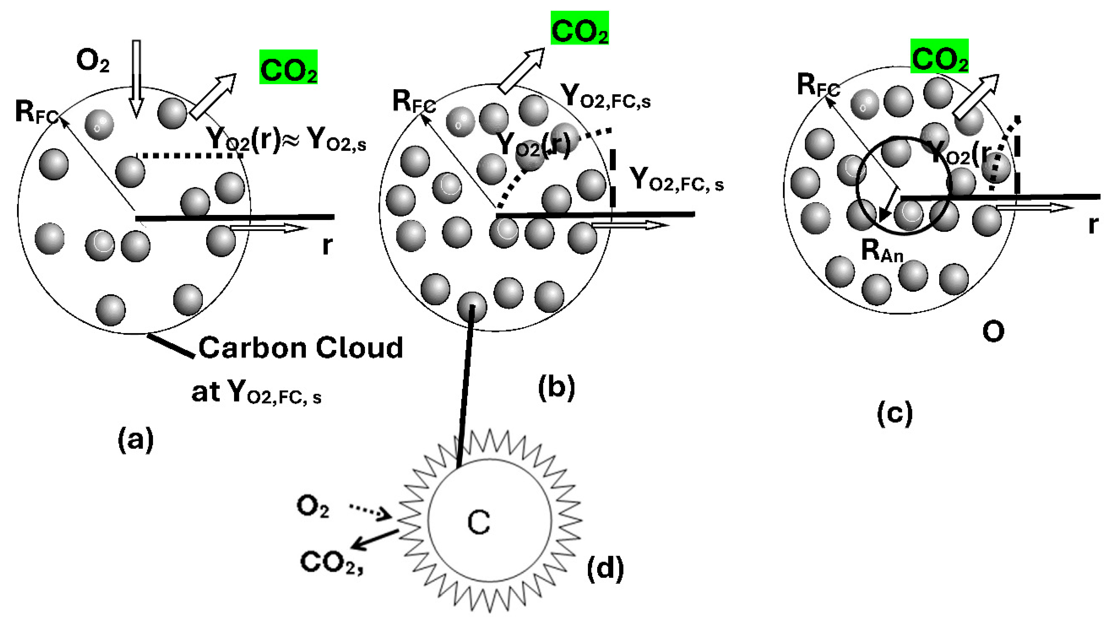
Figure 2.
Effectiveness Factor of organ k (ηeff or ηeff,k for organ k in biology) vs. G (or GOD, k for application to cell clouds in biology). For application to an organ k in a BS, particles are replaced by cells in the ODM model. I) Dilute Cloud: G < 1, within which ηeff ≈ 1, indicating all particles are exposed to the same surface oxygen concentration, or each particle releases energy as though it is isolated. II) Dense Cloud {1 < G < 100: Interactive Combustion Mode or ODC mode with a decreasing oxygen concentration within the cloud, III) Very Dense Cloud: G >100. Particles near the surface oxidize rapidly, while the center of the cloud contains very little oxygen, and particles at the core may not oxidize. The same plot is valid for cell clouds with ηeff, = ηeff,k, G = GOD,k. I) Dilute Cell Cloud: GOD,k < 1, within which ηeff ≈ 1, indicating all particles are exposed to same surface oxygen concentration or each cell releases energy as though it is isolated. II) Dense Cell Cloud: Crowding effects of cell or ODM mode with a decreasing oxygen concentration within the cloud, 1 < GOD,k < 100. III) Very Dense Cloud: GOD,k > 100.
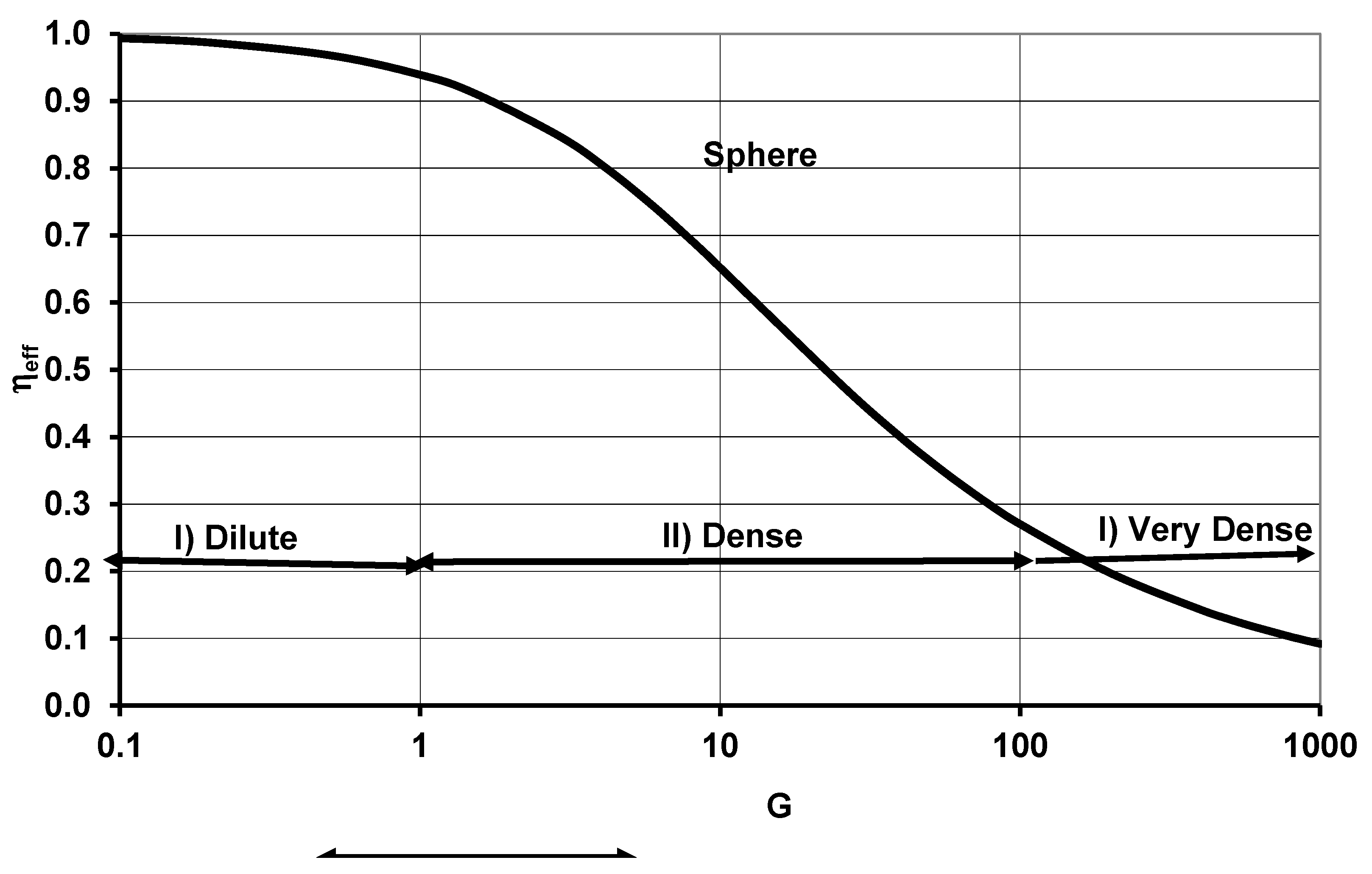
Figure 3.
a) Capillary system-Cells can be placed within a cylinder with capillary on axis ( COA) or cells can be enclosed by capillaries known as capillary on surface ( COS). The (COS) Model is known as the solid “cylinder” model in biology. Figure adopted from [02/27/2025, accessed on https://en.wikipedia.org/wiki/Capillary] and modified. b) COS model for spherical cloud of cells with cell located at “r” consuming O2 at the rate of ; capillaries are partly perfused { e.g Resting condition}. c) COS model with fully perfused capillaries {e.g exercise} for a spherical cloud of cells. COS model is close to ODC model in engineering literature. The O2 diffuses towards center of cell cloud (CC) of radius and mass mCC. Cells adjacent to the surface containing capillaries are aerobic, while those farther surface become hypoxic, and the farthest cells are necrotic cells. Detailed results for cell clouds are given in Column 4 of Table 2 in Ref. [3]. Certain regions within organs may undergo only glycolysis due to a lack of O2. (Adopted from Ref. [3]) with modifications.) Note that for the partly perused capillaries as shown in (b) as in the case of BS under rest, average oxygen mass fraction at the surface of CC , YO2,CC,s is low. When almost all capillaries are perfused {e.g exercise} as shown in (c ) , YO2,CC,s increases to a maximum.
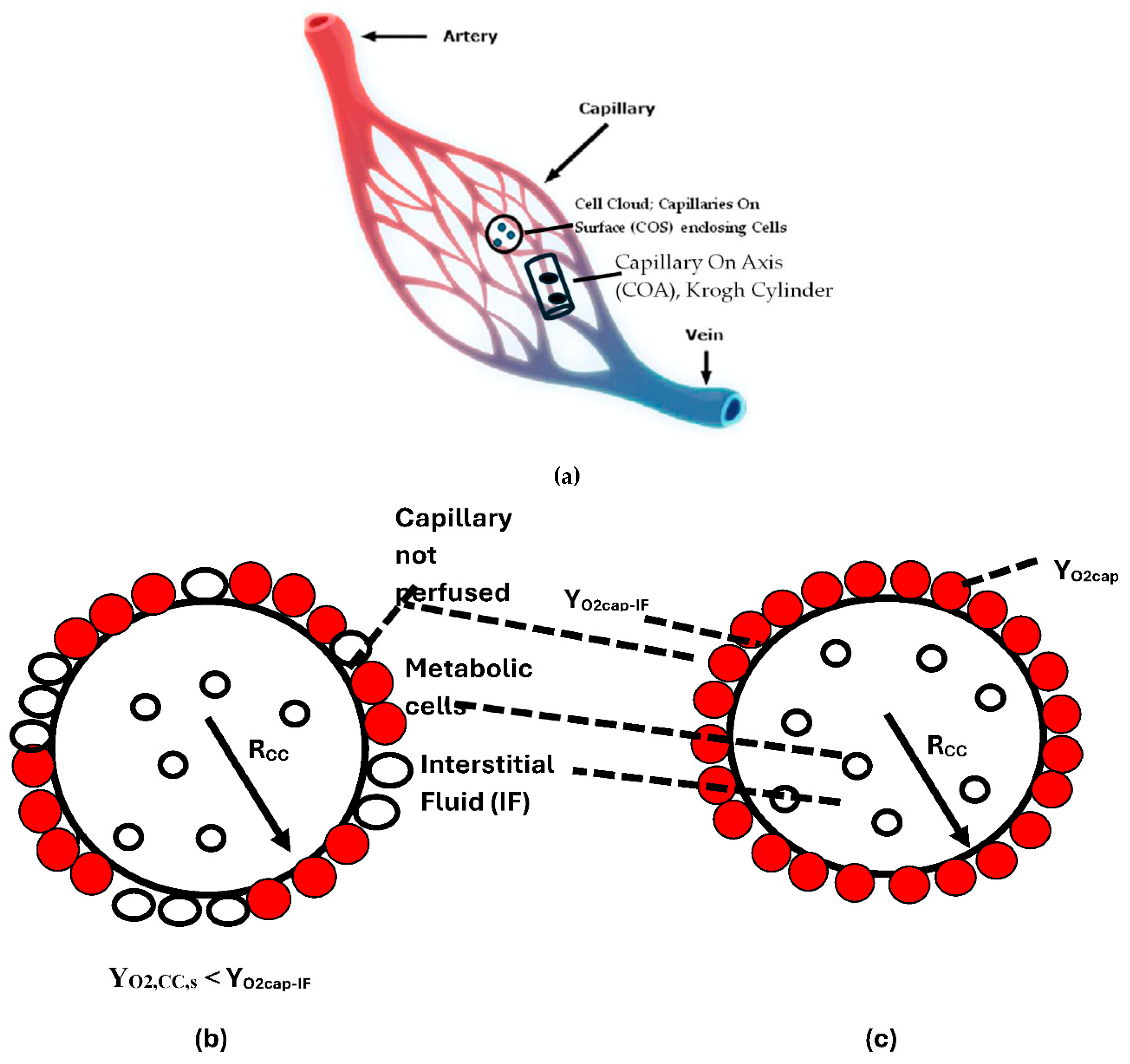
Figure 4.
The constants in SOrMRk relations were based on data from organ metabolic rates of six species ranging in mass from 0.48 kg to 70 kg. Whole-body metabolic rates of 116 species (ranging from 0.0076 to 6,650 kg), for which organ masses are known, were obtained by assuming the SOrMRk values derived from the six species are valid for the organs of all 116 species. Using these data and the known organ mases of the 116 species, whole-body metabolic rates were estimated for BS with body mass ranging from 0.0075 kg to 6,650 [21]. .
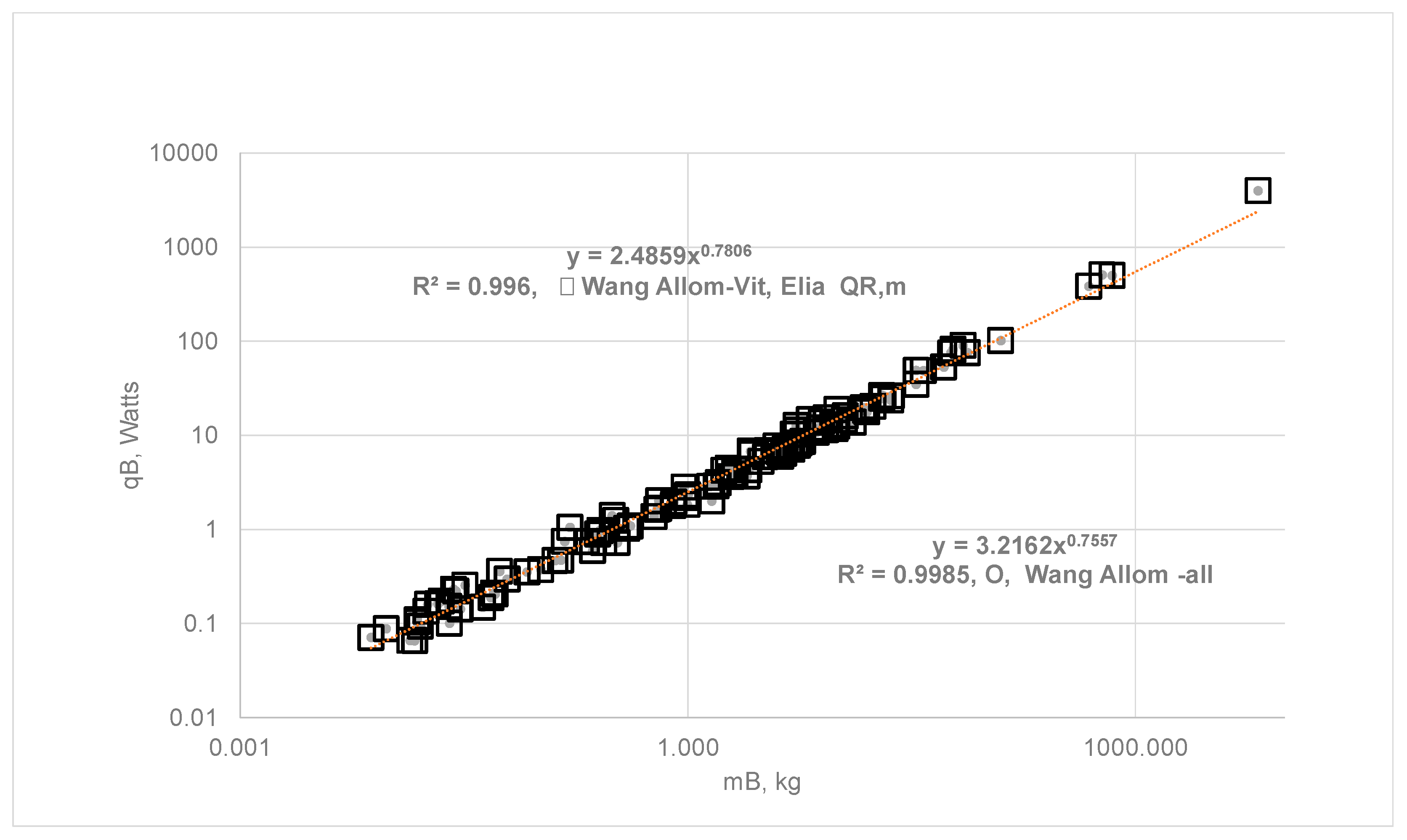
Figure 5.
Comparison of whole-body metabolic rate using the ODM Method (with RS-1 = 0.0076 kg RS-2 = 0. 390 kg and EAR for the organs; , MB = 0.0075 kg to 6,650) i) () ODM Method: a = 2.963, b = 0.747, ii) (O) EAR Method: a = 3.216, b = 0.756. Kleiber’s law constants are almost the same with both methods.
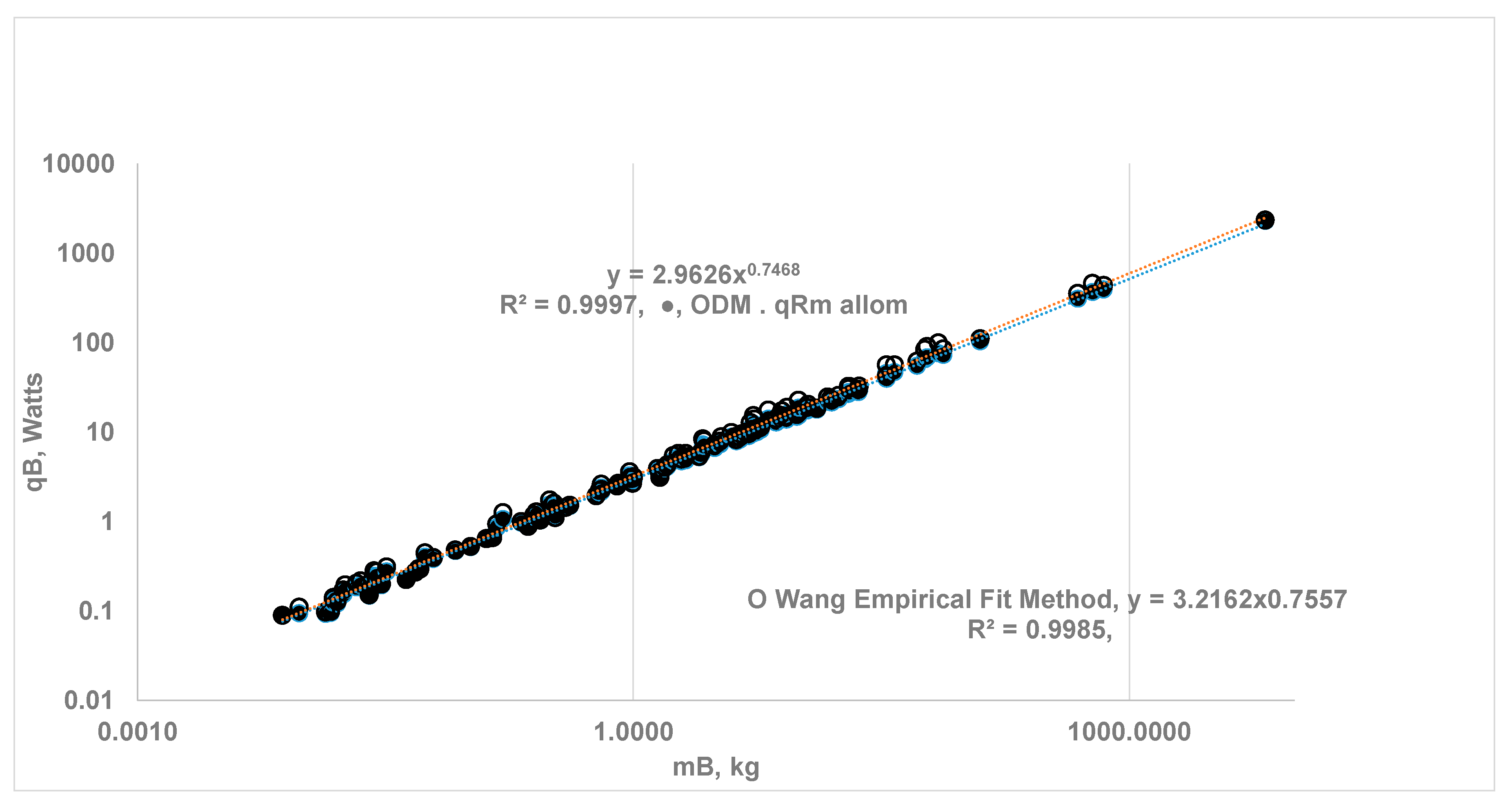
Figure 6.
Comparison of ODM based whole-body MR with EAR based MR for BS ranging in mass from 0.0075 to 6,650 kg. Kleiber’s law: i) from the allometric relation: a= 2.963 b= 0.747, ii) with Elia’s constant of 0.581 W/kg, a = 2.242, b = 0.772. The percentage increase in b for the ODM method is the same as the percentage increase in the EAR method when is changed from an allometric law to a constant value for 116 species.
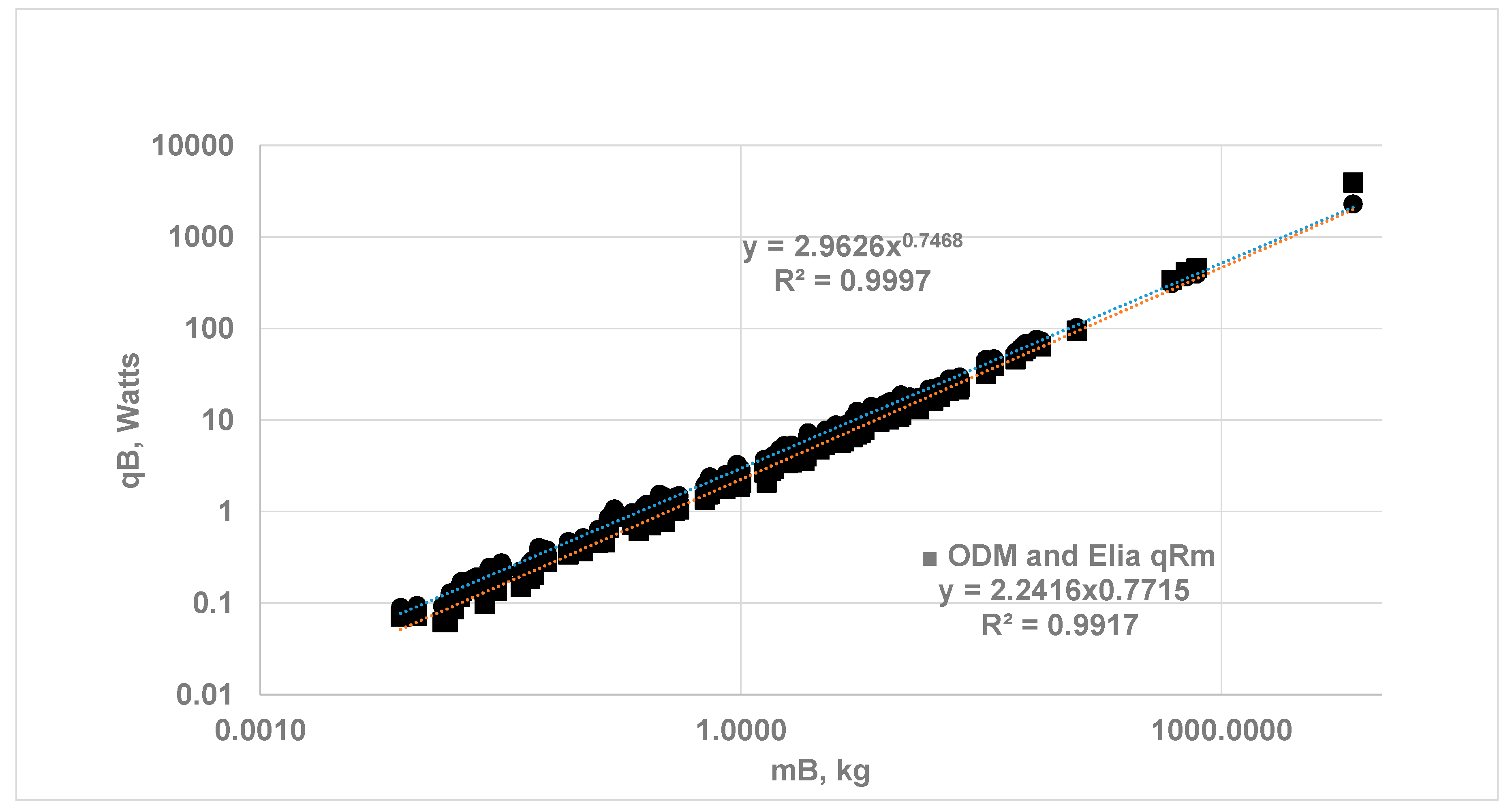
Figure 7.
ERR from vital organs and upper ERR (ηeff, k = 1 for vital organs) as a function of vital organ mass, mvit: Comparison between ODM and EAR data. Vital organ MR (ODM) for 116 with body mass ranging from 0.0076 kg to 6,650 kg; , in watts, mvit in kg. i) (■) ODM Method: αvit = 12.961, βvit = 0.737, ii) (O) EAR Method: αvit = 15.667, βvit = 0.767. under ODM are slightly lower compared to of EAR. iii) in watts when O2 gradients disappear for all vital organs (ηeff, k = 1 when ηeff, k = 1 for all vital organs) (▲): , αvit,UMR = 92.58, βvit,UMR = 1.009. For , the law is almost isometric with respect to vital organ mass since all cells in vital organs are exposed to uniform cloud surface oxygen concentration.
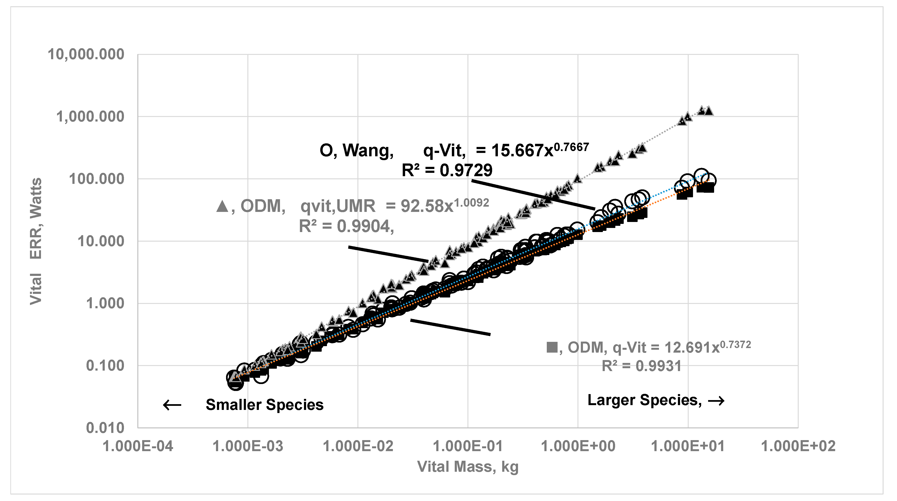
Figure 8.
Comparison of vital organ mass percentage and energy contribution percentage: ODM vs. EAR for all organs. Energy contribution percentage by vital organs: . From ODM method (■): γvit = 49.67, νvil = -0.115. From EAR for all vital organs (●) [21]: γvit = 51.85, νvil = -0.101. (▲) vital organ mass percentage = 45.376 MB -0.141.
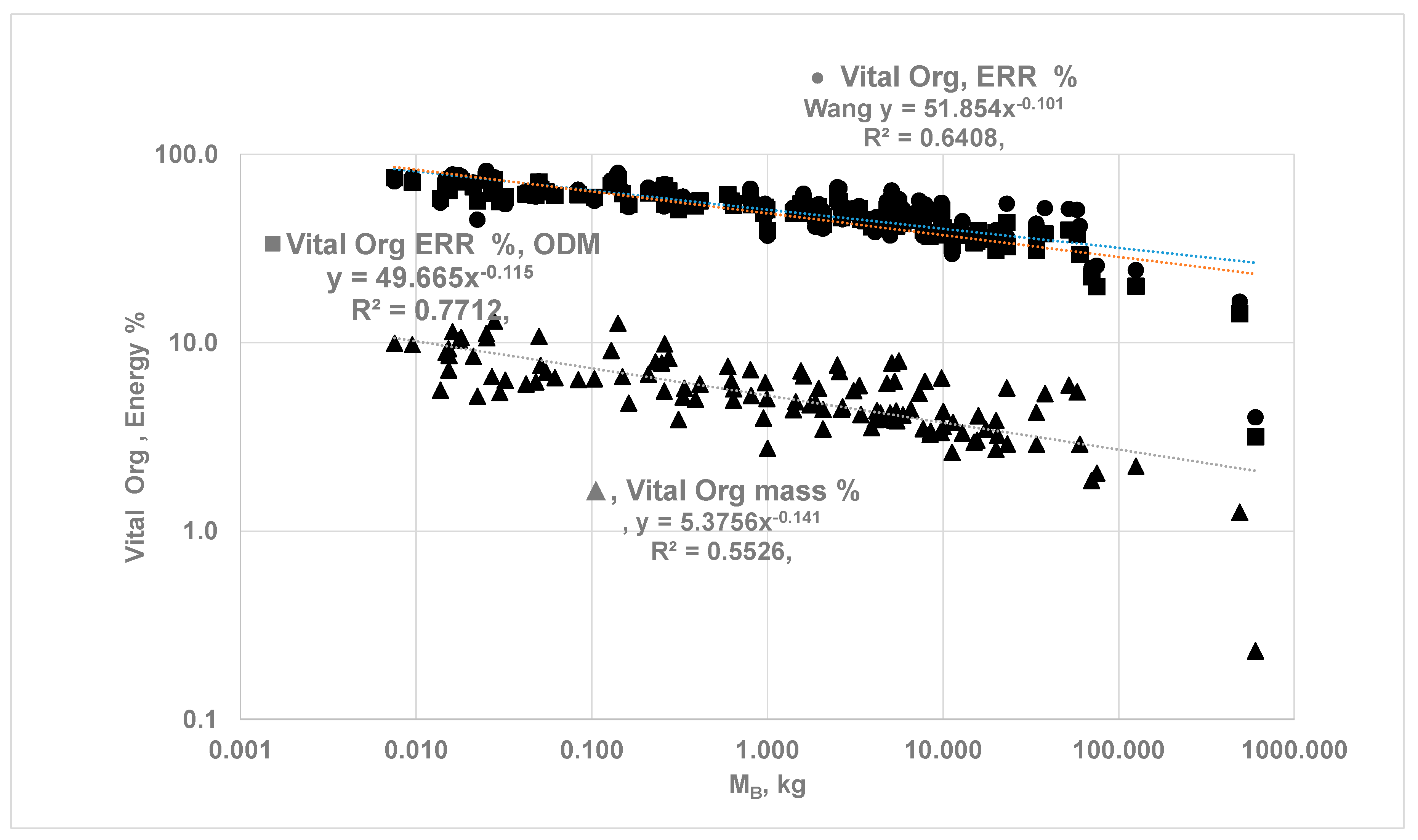
Figure 9.
Comparison of UMR of of BS (, ηeff = 1) with MMR of BS {, ηeff = 1, Perf. Ratio}. The ODM based BMR with finite ηeff,k yields Kleiber’s law: , all in Watts , , (■) aUMR = 6.282, bUMR = 0.864 with at isolated rates and following allometric law. The MMR vs MB is higher compared to UMR primarily due more perfusion of blood to SM and affected by YO2,CC,s at CC surface is affected by more capillary perfusion for SoMRk. With ,: aMMR = 8.436, bMMR =0.942.
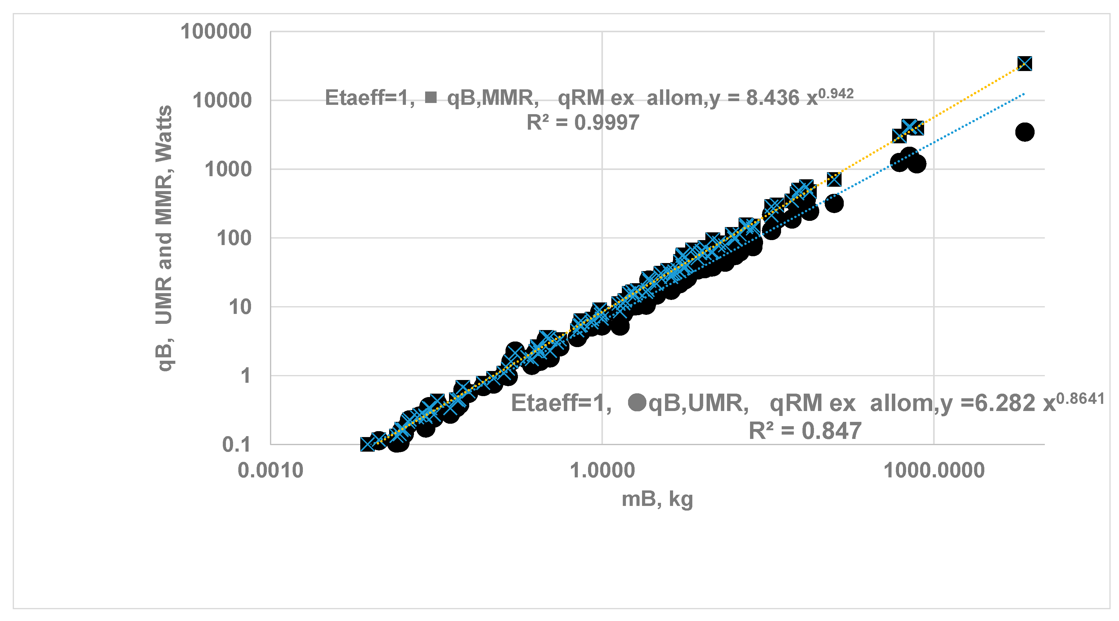
Figure 10.
Comparison of MMR (, ♦ and ●), with the literature data (▲) on MMR of BS vs. body mass, MB. MB from 0.01 to 10,000 kg . The ODM based BMR with finite ηeff,k yields Kleiber’s law: , all in Watts , MMR : a) allometry predicted ,SM mass in kg: mSM = 0.061 MB 1.09 [62] . m RM-Ex = MB - m vit - m SM . a) ♦ Vit organ with finite ηeff, and follow EAR, Perf. Ratio of Table 2 used, aSM= aRM bSM = bRM aMMR. = 4.015 bMMR = 0.798 , b) ● Assumed ηeff,k =1 for all vital organs and SM; RM-ex allom. Law of RM , aRM-ex= aRM, bRM-ex = bRM {Table 1}.., aMMR. =8.436 bMMR = 0.942, Painter data from Literature in VO2,max : assuming 1 mL of O2 releases 20.5 J, For Painter data , aMMR = 40.46 bMMR = 0.872.
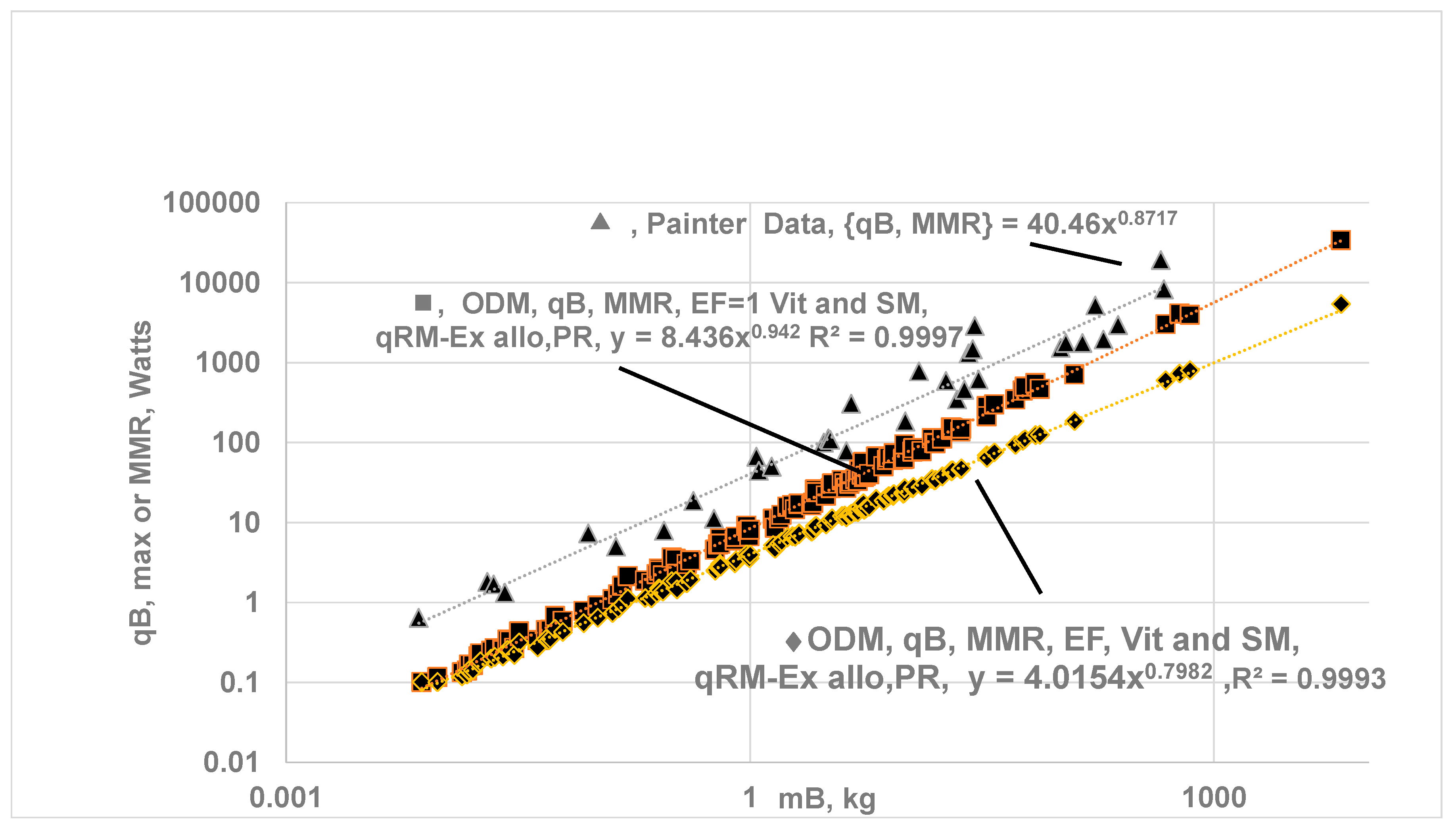
Table 1.
Allometric Constants for Organ Mass, Energy Release (Metabolic) Rate. Values are based on six species: Rat (0.45 kg), Rabbit (2.5 kg), Cat (3 kg), Dog (10 kg), Human-1 (65 kg), Human-2 (70 kg). (Adopted and modified from Wang–5 organ model, Table 4 of Ref. [29]). The body is composed of four vital organs, BrHKidL, with the fifth organ representing the rest of the mass of the body (RM). Constants ck,6, dk,6, ek,6 and fk,6 are from Ref. [21]; density from Ref. [22]).
| Organ | ρk, g/cc | ck,6, 1 kg | dk,62 | ek,6 3 | fk,6 4 | mk (85 kg human) | Ek,6 | Fk,6 | (85 kg human) | ck,116 [3] |
dk,116 [3] |
OEFk) 84 kg human) |
| Kidneys (Kids)5 | 1.05 | 0.007 | 0.85 | 33.41 | -0.08 | 0.31 | 20.94 | -0.094 | 0.11 | 0.00631 | 0.728 | 0.085 |
| Heart (H) | 1.06 | 0.006 | 0.98 | 43.11 | -0.12 | 0.47 | 23.04 | -0.122 | 0.15 | 0.00580 | 0.932 | 0.48 |
| Brain (Br) | 1.036 | 0.011 | 0.76 | 21.62 | -0.14 | 0.32 | 9.42 | -0.184 | 0.044 | 0.0108 | 0.886 | 0.37 |
| Liver (L) | 1.06 | 0.033 | 0.87 | 33.11 | -0.27 | 1.57 | 11.49 | -0.310 | 0.19 | 0.0286 | 0.872 | 0.52 |
| RM6 | 0.939 | 1.01 | 1.45 | -0.17 | 83.44 | 1.44 | -0.168 | 0.19 | 0.940 | 1.007 |
Table 2.
Capillary Perfusion Percentage Assumed for MMR. Note: Capillary perfusion percentage does not affect SOrMRk and BMR estimations; they affect only YO2,CC,s or MMR under exercise. Accessed 02182025 https://courses.lumenlearning.com/suny-ap2/chapter/homeostatic-regulation-of-the-vascular-system/.
| Organ | Rest (mL/min) | Mild Exer(mL/min) | Maximal (mL/min) | Rest % | Exercise % | EX-Rest ratios |
| Kidney | 1100 | 900 | 600 | 19 | 3 | 0.55 |
| Heart | 250 | 350 | 750 | 4 | 4 | 3 |
| Brain | 750 | 750 | 750 | 13 | 4 | 1 |
| Others (i.e., liver, spleen) | 600 | 400 | 400 | 10 | 2 | 0.67 |
| Skeletal muscle | 1200 | 4500 | 12500 | 21 | 71 | 10.42 |
| RM-Ex (GI+skin+others) | 2500 | 3000 | 2900 | 43 | 17 | 1.16 |
Disclaimer/Publisher’s Note: The statements, opinions and data contained in all publications are solely those of the individual author(s) and contributor(s) and not of MDPI and/or the editor(s). MDPI and/or the editor(s) disclaim responsibility for any injury to people or property resulting from any ideas, methods, instructions or products referred to in the content. |
© 2025 by the authors. Licensee MDPI, Basel, Switzerland. This article is an open access article distributed under the terms and conditions of the Creative Commons Attribution (CC BY) license (http://creativecommons.org/licenses/by/4.0/).
Copyright: This open access article is published under a Creative Commons CC BY 4.0 license, which permit the free download, distribution, and reuse, provided that the author and preprint are cited in any reuse.


