Submitted:
04 March 2025
Posted:
05 March 2025
You are already at the latest version
Abstract
To address the growing security risks posed by unauthorized UAV activities, this paper proposes a real-time two-dimensional direction-finding (DF) system for UAV based on radio frequency (RF) signals. The system employs a six-element uniform circular array (UCA), synchronized HackRF One receivers, and a hybrid algorithm integrating the multiple signal classification (MUSIC) method with a novel weighted average algorithm (WAA). By optimizing the MUSIC spectrum search process, the WAA reduces computational complexity by over 99.9% (from 3240000 to 1200 spectral function calculations), enabling real-time azimuth and elevation angle estimation. Experimental results demonstrate an average azimuth error of 7.0° and an elevation error of 7.7°, for UAV hovering distances of 30-200 m and heights of 20-90 m. Real-time flight tracking further validates the system’s dynamic monitoring capability. The hardware platform, featuring omnidirectional coverage (0-360° azimuth, 0-90° elevation) and dual-band operation (2.4 GHz/5.8 GHz), offers scalability and cost-effectiveness for low-altitude security applications. Despite limitations in elevation sensitivity due to UCA geometry, this work establishes a practical foundation for UAV monitoring, emphasizing computational efficiency, real-time performance, and adaptability to dynamic environments.
Keywords:
UAV monitoring
; direction-finding
; MUSIC algorithm
; weighted average algorithm
; uniform circular array
; real-time tracking
; radio frequency
1. Introduction
Unmanned aerial vehicles (UAVs), as a type of unmanned aircraft, have now developed into high-tech products with highly intelligent and diversified functions. Their applications span diverse fields: in agriculture, UAVs are used for farmland mapping, turfgrass monitoring, and pesticide spraying, improving the efficiency and quality of agricultural production [1,2,3]; in the logistics industry, UAV delivery models are being explored to enhance the speed and coverage of logistics distribution [4]; in film and television production, UAV aerial photography provides audiences with stunning aerial perspective images [5,6]. With their rapid response and flexible maneuverability, UAVs provide efficient and convenient solutions for various industries, profoundly impacting many aspects of modern society. UAVs continue to expand their application boundaries, showing broad prospects for development.
However, the rapid proliferation of UAV technology has introduced significant challenges to public safety and privacy. Malicious actors are increasingly exploiting UAVs for unauthorized surveillance, airspace intrusions near critical facilities, and raising concerns about privacy breaches and airspace security [7]. UAVs have been used to conduct unauthorized aerial photography of private properties, government buildings, and military installations, posing a serious threat to individual privacy and national security [8].
These threats underscore the urgent need for robust UAV monitoring systems. UAV monitoring encompasses detection, identification, and localization, where direction-of-arrival (DOA) estimation serves as a key component of localization and countermeasure deployment. Accurate DOA estimation is crucial for determining the position and trajectory of UAVs, enabling timely interventions to mitigate potential risks. Current direction-finding (DF) methods rely on acoustic, radar, radio frequency (RF), and visual technologies [9,10,11,12]. Among these, RF-based systems strike a balance between operational range, cost-effectiveness, and adaptability to dynamic environments [13]. RF signals emitted by UAV controllers or onboard communication modules provide a reliable source for passive detection, making them particularly suitable for covert monitoring scenarios [14].
To this extent, we propose a DF system for UAVs based on RF signals. The system utilizes a uniform circular array (UCA) to receive UAV signals and combines the multiple signal classification (MUSIC) algorithm with the weighted average algorithm (WAA) to estimate the direction, effectively measuring the UAV’s azimuth and elevation angles. The experiments validate the system’s robustness: for the hovering experiment, achieving average azimuth and elevation errors of and , respectively; for the real-time measurement experiment, the system shows effective tracking ability, providing reliable UAV monitoring information.
The rest of this paper is structured as follows: Section 2 reviews related work on UAV DF methods based on RF signals; Section 3 details the proposed method combining the MUSIC algorithm with the WAA algorithm; Section 4 describes the DF system’s hardware and software components; Section 5 presents the measurement results and analysis; finally, Section 6 concludes the paper with a summary and future work.
2. Related Work
In [15], the authors propose a UAV direction positioning method leveraging sparse denoising autoencoders (SDAE) and deep neural networks (DNN). This approach enables implementation without requiring phase synchronization, antenna calibration, or detailed analysis of antenna radiation patterns, and can be executed using a single-channel RF receiver. Experimental results show that the proposed method achieves resolution for UAV azimuth estimation.
Recent research on UAV direction-finding (DF) systems has made significant advancements, particularly in array signal processing techniques. In [16], the authors propose a subspace tracking algorithm with low computational complexity for tracking the DOA of an Internet of Things (IoT) based UAV using QR factorization and Givens rotation methods to compute the inverse of a matrix. Simulation experiments show that the proposed algorithm can track the signal source successfully, and its performance is comparable to that of the DOA estimation and beamforming algorithm.
In [17], the authors utilized a UAV remote controller as the FHSS signal source. The signal is received through a four-element uniform linear array (ULA) and preprocessed by time-frequency analysis and reconstruction. The MUSIC algorithm and root-MUSIC algorithm are used to estimate the DOA of the signal. Comparison tests proves that the proposed method has significantly improved the accuracy of DF, and the average error of DOA estimation is .
Research in [18] showed that the authors, based on the software-defined radio (SDR) platform, used the Universal Software Radio Peripheral (USRP) series of hardware devices along with a 4-element uniform linear array. They processed the signals received by four phase-coherent RF channels with the MUSIC algorithm and evaluated the DF estimation performance by comparing the directions in the UAV’s flight log with the directions estimated by the DF test platform. The experiment results showed that in a static scene, the average estimation error was , and in a dynamic scene, the average estimation error was .
The article in [19] presents a UAV tracking device based on a 4-element uniform linear array which operates within a DOA range from to . By comparing with the root mean square error (RMSE) of different DOA estimation algorithms (such as DS, Capon, MUSIC, ESPRIT, and Tensor), it is concluded that the preprocessed DS algorithm has the smallest RMSE. The maximum DOA error is , and the average DOA error is .
In paper [20], the authors propose a USRP-based UAV positioning system that uses a five-element UCA antenna and a MUSIC algorithm to determine the azimuth DOA of the UAV. A DJI Mavic 3T-Basic Enterprise UAV was used as a target, with the UAV hovering at 14 different locations. Compared to the actual DOA calculated from the UAV log file, the average error is , the minimum error is , and the maximum error is .
Existing research on DOA estimation focuses on array configurations, algorithmic enhancements, and hardware implementations, yet critical gaps remain in elevation angle estimation, range of DF, and computational efficiency. ULA is widely used for its simplicity, compatibility, and mature algorithms. However, ULA inherently limits DF to 0- and cannot resolve the forward and backward direction of the estimated angle, limiting its utility in complex 3D airspace monitoring. To overcome these limitations, UCA has been explored for azimuth detection in all directions. However, related studies still have shortcomings in elevation angle measurement.
Based on the aforementioned limitations, we propose a DF system based on a UCA combined with the MUSIC algorithm and the WAA. Unlike previous methods that use ULA, our UCA configuration enables omnidirectional signal reception. Moreover, we achieve the real-time estimation of the azimuth and elevation angles of the UAV, addressing the shortcomings of existing 2D DOA estimation. Additionally, integrating the WAA algorithm optimizes the MUSIC spectrum, significantly improving DF accuracy and computational efficiency. Our system also demonstrates robust performance in real-world environments, making it a practical and reliable solution for UAV monitoring. The main contributions of this research can be summarized as follows:
- A novel DF system is proposed by integrating a UCA with the MUSIC and WAA hybrid algorithm. This hybrid approach optimizes the MUSIC spectrum search process, reducing computational complexity by more than 99.9% compared with spectral traversal (from 3240000 to 1200 spectral function calculations), while achieving real-time azimuth and elevation estimation;
- A scalable and cost-effective hardware platform is developed using six HackRF One software-defined radio devices, synchronized via synchronization clock and trigger modules. The system supports omnidirectional coverage (0- azimuth, 0- elevation) and dual-band operation (2.4 GHz and 5.8 GHz) by replacing the antenna array;
- Through the UAV hovering experiment (30-200 m distance, 20-90 m altitude), it demonstrates the DF system’s accuracy, with average azimuth and elevation errors of and , respectively. By comparing real-time data, the effective tracking ability of the DF system for UAV is verified.
3. Proposed Method
In this section, we explore the application of the swarm intelligence optimization algorithm WAA [21] to optimize the MUSIC spectrum function for direction-of-arrival (DOA) estimation. The MUSIC algorithm [22] is known for its high-resolution DOA estimation capabilities, but its computational inefficiency in the spectrum search process can limit its real-time application. To address this issue, the WAA is integrated with the MUSIC algorithm to improve optimization efficiency and reduce computational time.
3.1. MUSIC Algorithm Based on UCA
As illustrated in Figure 1, this is a uniform circular array (UCA) with M elements, where the radius of the array is R and its center serves as the reference point. Assuming a far-field narrowband signal with a carrier frequency arriving at the UCA from the direction . The signal can be expressed in its complex form as follows:
where denotes the complex envelope of , which exhibits a slow temporal variation.
Define the propagation delay for each array element m with respect to the reference point as , for . If the signal received at the reference point is , the signal received by the m-th element of the array is:
Let and , where is the wavelength. The position of the m-th array element is:
And the unit vector pointing in the direction of signal arrival is:
Thus, the propagation delay for the m-th array element relative to the reference point is given by:
Where c is the speed of light, and the corresponding phase shift is:
The steering vector for the direction of arrival (DOA) is defined as:
For K narrowband signals arriving at the UCA with corresponding DOAs , the received baseband signal at the array can be expressed as:
where is the array response matrix, and denotes the additive white Gaussian noise.
The MUSIC algorithm relies on the eigenvalue decomposition of the covariance matrix . After decomposing the matrix, the MUSIC pseudospectrum is defined as:
Where is the noise subspace from . The peaks of this spectrum correspond to the directions of arrival (DOAs) of the received signals.
3.2. Weighted Average Algorithm
The weighted average algorithm is a novel metaheuristic optimization technique that aims to balance exploration and exploitation. The core idea behind this algorithm is to iteratively adjust the search parameters and calculate the weighted average position. This process helps guide the optimization and makes the WAA suitable for solving complex optimization problems in various domains, including DOA estimation. The optimization process involves the following key steps:
(1) Initialization phase
This phase randomly generates an initial set of candidate solutions and calculates the fitness value of each candidate solution. The set of candidate solutions is denoted as matrix , which is defined by equation 10 and randomly generated within the predefined search space according to equation 11.
Where denotes the position of the i-th solution within the j-th dimension, N denotes the total number of candidate solutions, and n denotes the dimensionality of the problem.
Where is a random number between 0 and 1, denotes the j-th lower bound value, and denotes the j-th upper bound value of the given problem.
(2) Weighted average position
To determine the weighted average position, the initial step involves evaluating the fitness of each participant. Next, the candidate solutions are re-organized based on one of two optimization goals: the larger the better (LTB) or the smaller the better (STB). If LTB, sort the candidate solutions from larger to smaller fitness values, while if SLB, sort the candidate solutions from smaller to larger fitness values. Following this, the first candidates from the set of candidate solutions are chosen to calculate the weighted average position, utilizing the equations provided below:
Where is the number of populations, is the i-th candidate solution, is the function used to calculate the fitness value, is the total of all fitness values from the chosen candidates, and is the weighted average position. Additionally, is the current iteration number, and is the maximum iteration limit. is the number of selected candidate solutions.Notably, Equations 14 and 15 correspond to the weighted average position equations when choosing the optimization goals of STB or LTB, respectively.
(3) Defining the search phase: exploration or exploitation
For each candidate solution in the population, it is decided whether to explore or exploit according to Equation 16.
Where is a random value ranging from 0 to 1, and is an adjustable constant to control the balance between the exploration and exploitation phases.
(4) Exploitation phase
The exploitation strategy simulates how the population of search agents moves towards the search spaces with a high probability of exploiting new global best values. There are three movement strategies employed during the exploitation phase, which are detailed in the following equations. Each of these formulas represents a distinct exploitation strategy.
Where are random values ranging from 0 to 1, and represent the personal best and global best position in the iteration numbers, respectively.
(5) Exploration phase
The exploration phase aims to identify novel potential solutions across the global domain, thereby enhancing population diversity and avoiding falling into local optima. There are two different exploration strategies during the exploration phase. The first strategy is based on the Lévy’s flight model, which is defined by the following equations:
Where represents the Gamma distribution function, while S is the step length of the Lévy flight, which is influenced by the parameter .Additionally, U and V satisfy normal distributions with standard deviations equal to and respectively, and both have a mean of 0. During the Lévy flight process, the step length is determined by the value of . The notation is the j-th position in the global best solution at iteration iter, whereas denotes the j-th position of the i-th solution at iteration .
The second exploration strategy is defined by the following equation:
Where and represent the lowest values of the lower and upper bounds across all dimensions, respectively.
To better illustrate the optimization process, a flowchart summarizing the steps is shown in Figure 2. It can be seen that the main process of the WAA algorithm includes three parts: initialization, recording the optimal solution, and updating the population. The core aspect lies in the calculation of the weighted average position and the balance between the exploration and exploitation phases. The exploration phase enhances global search ability through two exploration strategies, while the exploitation phase improves local optimization ability through three exploitation strategies. After several iterations, the WAA algorithm can find the precise optimal solution of the objective function.
3.3. Simulation of MUSIC Spectrum Function Optimization Based on WAA
We investigate DOA techniques for a single UAV. In this context, the MUSIC spectrum function exhibits its peak in the direction of arrival of the UAV RF signal source. Using this characteristic, we reformulate the DF problem for a single UAV as an optimization problem, specifically focusing on identifying the maximum value of the MUSIC spectrum function to determine the DOA of the corresponding UAV RF signal. To convert this optimization problem into a minimization problem (usually optimization algorithms are used to solving the minimum optimization), we multiply the MUSIC spectrum function by -1. Thus, the optimization problem becomes:
subject to:
Where and denote the elevation and azimuth angles, respectively, in the MUSIC spectral function.
To verify the optimization effect of the WAA algorithm on the MUSIC spectrum function, MATLAB simulation experiments were carried out. A 2.4 GHz incident signal with an arrival angle of in azimuth and in elevation and a signal-to-noise ratio (SNR) of 5 was set for the experiment. The receiving array is a 6-element UCA with a radius of 6.25 cm. The population size of the WAA algorithm is set to 30, the number of iterations is set to 40, and the WAA parameter = 10.
To assess the performance of WAA, we compare it with other popular optimization algorithms, such as the Whale Optimization Algorithm (WOA)[23], Sparrow Search Algorithm (SSA)[24], Particle Swarm Optimization Algorithm (PSO)[25], and Grey Wolf Optimization Algorithm (GWO)[26]. All algorithms are tested under the same simulation conditions, with identical population sizes and iteration numbers. The optimal fitness curves for different optimization algorithms across iterations are shown in Figure 3.
The WAA algorithm significantly outperforms other optimization algorithms, converging to the optimal solution in fewer iterations. Specifically, WAA completed the optimization within just 5 iterations (where the MUSIC spectrum function evaluated 1200 times during the 40 iterations), reducing computation time by approximately 99.9% compared to the traditional MUSIC spectrum traversal method that searches at every increment (where the MUSIC spectrum function was evaluated 3240000 times).
The optimized azimuth and elevation angles obtained using the WAA are and , respectively. The corresponding value of the objective function is -538.745, demonstrating high optimization accuracy. These results illustrate that the WAA algorithm not only enhances the computational efficiency of the MUSIC algorithm but also maintains excellent precision in estimating the DOA.
4. DF System Description
The proposed DF system, as illustrated in Figure 4, comprises five core components: a UCA antenna array, a HackRF One[27] receiver group, a synchronous clock module, a synchronous trigger module, and a host controller. These components work in concert to enable real-time reception and processing of UAV RF signals, allowing for the accurate estimation of DOA and the tracking of UAV movement.
The UAV RF signal is received through the UCA antenna units and transmitted to the corresponding HackRF One unit via RF lines of the same length. The group of HackRF One receivers achieve synchronous signal reception through the synchronous clock and trigger modules. The host controller performs phase calibration on the received multi-channel signals, followed by real-time calculations, with the results displayed via the GUI module.
(1)UCA antennas
The UCA antennas are the system’s primary signal reception component. They consist of six 2.4 GHz folded dipole antennas arranged in a circular configuration with a radius of 6.25 cm (corresponding to half-wavelength spacing for 2.4 GHz signals, which have a wavelength of 12.5 cm). The antenna array operates within the 2.4 GHz frequency band, providing a gain of 6 dBi per antenna. This configuration enables omnidirectional reception of RF signals while maintaining phase coherence across all antenna elements, which is crucial for accurate DOA estimation.
(2)HackRF One Receiver Group
The HackRF One receiver group comprises six individual HackRF One software-defined radio (SDR) devices, each connected to a corresponding antenna element in the UCA. The HackRF One is a versatile SDR that supports a frequency range of 1 MHz to 6 GHz, with a maximum analog-to-digital conversion (ADC) sampling rate of 20 MSPS. This wide frequency range makes it well-suited for receiving UAV communication signals which typically operate in the 2.4 GHz and 5.8 GHz bands. To ensure synchronized operation of the receiver devices, a common clock source is shared across all HackRF One units. This synchronization is essential for accurate phase calibration and signal processing, as phase discrepancies between channels could otherwise lead to inaccurate DOA estimations.
(3)Synchronous Clock Module
The synchronization clock module is an 8-channel, 10 MHz square wave generator (BG7TBL) that provides a unified reference clock for all HackRF One units. This ensures that all devices operate at the same sampling rate, allowing for consistent data acquisition across the receiver channels.
(4)Synchronous Trigger Module
The synchronization trigger module is implemented using an Altera EP4CE10E22 FPGA core board. This module generates a 5-pulse-per-second (PPS) rising-edge signal to synchronize the timing of data acquisition across all SDR devices. The synchronization trigger ensures that all signals are captured at precisely the same moments, thus eliminating timing mismatches between channels.
(5)Host Controller
The host controller integrates several functional modules developed using the GNU Radio framework, facilitating the real-time reception and processing of signals. There are four key modules are implemented on the host controller. The signal receive module collects the raw in-phase and quadrature (IQ) data streams from the HackRF One receivers. The phase calibration module compensates for phase discrepancies between different channels by referencing a calibration signal. The MUSIC&WAA DOA module implements the Multiple Signal Classification (MUSIC) algorithm for DOA estimation, further optimized by WAA to enhance the accuracy and computational efficiency of the system. The WAA optimization reduces the computational burden typically associated with MUSIC spectrum traversal, enabling real-time processing; The GUI display module provides a user interface for real-time monitoring of system performance. It displays the calculated DOA values and system status, providing a visual representation of the UAV’s estimated angles.
The physical components of the system is shown in Figure 5. The UCA antennas are mounted on a tripod at a height of 120 cm. The HackRF One receiver group receives the signal from the corresponding antenna. The FPGA-based synchronization modules ensure precise hardware synchronization across the receiver devices, while the GNU Radio software stack facilitates low-latency signal processing. The combined system provides real-time DOA estimation, enabling dynamic UAV tracking during flight.
5. DF System Description
5.1. System Initialization
Before conducting the experiments, the system was initialized to ensure optimal performance during data collection. Several parameters were configured, taking into account the limited processing throughput of the host computer. The sampling rate of the HackRF One devices were set to 2 MHz, and the center frequency was fixed at 2407 MHz. Additionally, the intermediate frequency gain and variable gain amplifier were both set to 30 dB to enhance signal reception sensitivity.
For the MUSIC algorithm, the following parameters were configured: the number of snapshots was set to 10,240; the number of antenna array elements was set to 6; and the radius of the array elements was 6.25 cm; and the number of sources was set to 1 to match the single UAV being tracked. These parameters ensured that the MUSIC algorithm could accurately process the signals received from the UAV.
In parallel, the WAA parameters were set as follows: the population size was set to 30, the number of iterations set to 30, and the WAA parameter was set to 10. These settings were selected to balance algorithm performance and computational efficiency.
Once the system parameters were configured, a phase calibration procedure was performed to address any hardware-induced phase discrepancies. This calibration step was essential to synchronize all receiver channels, ensuring accurate signal processing. A continuous radio wave signal at 2.407 GHz was used as the calibration source. The calibration signal was positioned 6 meters to the east of the UCA, aligned with the 0-channel antenna, ensuring that the antenna array was in the far-field region and met the necessary conditions for the calibration. As depicted in Figure 6, this process established a baseline for phase synchronization across all receiver channels.
The calibration process adjusted the phase difference between each channel to the correct value. Since the calibration signal is located in the same plane as the UCA, the wave path difference between the signals received from channels 1,2,3,4 and 5 relative to channel 0 should be , , , , and , respectively, and the corresponding phase difference is , , , , . The phase discrepancies between the channels were compensated for by the phase calibration module in the host computer, thereby ensuring that the system was ready for accurate direction-finding measurements.
5.2. Experimental Setup
The experimental site is located in the suburbs with less radio signal interference. The DJI AIR 2S commercial UAV (DJI, Shenzhen, China) [28], selected for its representative RF characteristics and operational versatility, was employed as the target UAV in this study.The DJI AIR 2S features configurable downlink signals operating within the 2.4 GHz and 5.8 GHz transmission bands. It offers a maximum transmission range of 12 km and a flight duration of approximately 30 minutes.
In addition, DJI AIR 2S provides detailed flight logs, including latitude, longitude, and altitude. These logs were essential for calculating the true azimuth and elevation angles, serving as a benchmark for evaluating the performance of the DF system. The experimental scene and the DJI AIR 2S are shown in Figure 7.
For the experiments, the signal characteristics of the UAV were set as follows: the bandwidth was 10 MHz, with a center frequency of 2.407 GHz. The waveform, spectrum, and waterfall diagram of the UAV’s RF signal are shown in Figure 8. As shown in Figure 8, the UAV’s RF signal exhibited discontinuous and irregular signal patterns within the 2.407 GHz band.The signal’s bandwidth and center frequency allowed for effective reception and processing by the HackRF One receiver, ensuring compatibility with the HackRF One receiver’s configuration.
During the experiment, the UAV operated at varying distances, ranging from 30 meters to 200 meters from the UCA receiving system, and at altitudes between 20 meters and 90 meters. These parameters provided a comprehensive simulation of typical monitoring scenarios, including both near-field and far-field conditions, as well as low- and medium-altitude scenarios. The flight paths for the two test flights are depicted in Figure 9.
All 26 hover flight positions of the two flights are shown in Figure 10. The positions of the two hover flights are indicated by different markers, and are distinct from the flight origin markers. The blue raindrop marker represents the hover point of the first flight, the purple circular marker represents the hover point of the second flight, and the orange circle represents the take-off point of the UAV. The azimuth is in the east direction and increases in a counterclockwise direction, the elevation angle is in the normal direction of the horizontal plane.
Each flight test involved the UAV hovering at distinct locations, with a minimum hovering duration of 10 seconds per position. This ensured that sufficient data were collected for accurate angle measurement. Notably, the UAV’s takeoff position was fixedat 0.5 meters away from the antenna array, and for the purposes of this experiment, the array was considered co-located with the UAV takeoff point. This arrangement enabled consistent and reliable measurements across the flight experiments.
5.3. Analysis of Angle Measurement of UAV Hovering Point
The angle measurements of the UAV hovering points were obtained by comparing the real-time direction finding (DF) system results with the angles calculated from the UAV’s flight log. The longitude, latitude, and altitude of each hovering point were extracted from the flight logs, and the distance and height differences from the starting point were calculated, as shown in Table 1. The UAV’s hovering positions, indexed from 1 to 26, were grouped into two distinct flight sequences. The first flight sequence consisted of 15 hovering points, while the second flight sequence had 11. Index 0 in Table 1 represents the UAV’s takeoff and landing point.
The distance between the 26 hovering points ranged from 30 meters to 200 meters, and the altitude varied between 30 meters and 90 meters. These variations in distance and height influenced the signal arrival direction, resulting in changes in the azimuth and elevation angles. The azimuth angle was computed from the UAV’s flight log using the Vincenty formula [29], and the elevation angle was calculated using the inverse tangent function.
The measurement results for each floating point are obtained by averaging the calculation results stored locally by the DF system during the UAV’s hovering period, after excluding outliers. The identification of outliers is based on a median absolute deviation (MAD) criterion, defined as data points differing by more than three times the median deviation. The measurement results are presented in Table , which contains the count of measurement results, the average value of the results, the percentage of outliers, and the absolute error compared to the angle values calculated from the UAV flight log.
As indicated in Table , the maximum error for the azimuth angles measured across the 26 UAV hovering points was , while the minimum error was , the average azimuth measurement error was . For the elevation angles, the maximum error was , the minimum error was , and the average error was . A notable outlier was observed at the 11th measurement point, where both azimuth and elevation errors substantially exceeded the average values more than 10 times. This can be attributed to the extended propagation distance causing signal attenuation, low SNR resulting in measurement errors, and severe multipath interference induced by shrubbery and experimental equipment along the transmission path. But this outlier is primarily caused by a period of coherent signal interference present in the environment, while other test points did not show such significant errors.

Table 2.
Comparison of measured azimuth and elevation angles from the DF system and calculated values from the UAV flight log.
Table 2.
Comparison of measured azimuth and elevation angles from the DF system and calculated values from the UAV flight log.
| Index | UAV flight log | DF system | Absolute error | |||||
| Azimuth (°) |
Elevation (°) |
Azimuth (°) |
Elevation (°) |
Count | Outliers (%) |
Azimuth (°) |
Elevation (°) |
|
| 0(start) | - | - | - | - | - | - | - | - |
| 1 | 169.7 | 45.1 | 162.6 | 36.5 | 6973 | 11.09 | 7.1 | 8.6 |
| 2 | 132.6 | 50.7 | 142.3 | 44.2 | 6034 | 4.21 | 9.7 | 6.5 |
| 3 | 142.8 | 53.3 | 142.8 | 57.4 | 3759 | 4.52 | 0.1 | 4.1 |
| 4 | 163.8 | 45.2 | 166.5 | 42.9 | 6837 | 25.82 | 2.7 | 2.3 |
| 5 | 166.5 | 48.4 | 168.1 | 35.9 | 3085 | 3.95 | 1.6 | 12.5 |
| 6 | 149.4 | 48.1 | 134.9 | 24.6 | 5096 | 9.52 | 14.5 | 23.5 |
| 7 | 153.6 | 56.4 | 154.6 | 60.5 | 5508 | 5.52 | 1.0 | 4.1 |
| 8 | 175.3 | 58.1 | 167.4 | 60.0 | 2818 | 4.05 | 7.9 | 1.9 |
| 9 | 177.3 | 66.7 | 176.9 | 72.6 | 3753 | 18.55 | 0.4 | 5.9 |
| 10 | 164.6 | 70.7 | 157.3 | 81.1 | 4296 | 2.89 | 7.3 | 10.4 |
| 11 | 155.3 | 66.0 | 46.5 | 28.9 | 3748 | 1.70 | 108.8 | 37.1 |
| 12 | 155.2 | 60.7 | 153.9 | 77.2 | 3631 | 5.48 | 1.3 | 16.5 |
| 13 | 180.9 | 60.5 | 181.4 | 57.7 | 4030 | 11.34 | 0.5 | 2.8 |
| 14 | 167.5 | 60.0 | 170.6 | 79.6 | 3618 | 12.24 | 3.1 | 19.6 |
| 15 | 125.5 | 45.0 | 124.8 | 61.9 | 4022 | 14.00 | 0.7 | 16.9 |
| 16 | 90.1 | 37.0 | 100.5 | 30.7 | 1745 | 3.04 | 10.4 | 6.3 |
| 17 | 133.1 | 50.5 | 143.3 | 50.3 | 4820 | 13.86 | 10.2 | 0.2 |
| 18 | 116.5 | 56.5 | 124.4 | 55.8 | 2810 | 11.10 | 7.9 | 0.7 |
| 19 | 88.0 | 48.5 | 107.7 | 38.1 | 2814 | 9.70 | 19.7 | 10.4 |
| 20 | 87.5 | 53.6 | 98.1 | 51.1 | 2143 | 6.07 | 10.6 | 2.5 |
| 21 | 110.3 | 55.5 | 118.9 | 65.5 | 2954 | 9.31 | 8.6 | 10.0 |
| 22 | 105.0 | 64.9 | 115.4 | 69.0 | 3754 | 4.05 | 10.4 | 4.1 |
| 23 | 118.7 | 68.7 | 128.3 | 66.8 | 3350 | 5.04 | 9.6 | 1.9 |
| 24 | 114.7 | 63.2 | 123.0 | 64.0 | 2682 | 4.88 | 8.3 | 0.8 |
| 25 | 98.1 | 57.6 | 108.2 | 50.5 | 3887 | 9.67 | 10.1 | 7.1 |
| 26 | 71.2 | 53.8 | 82.3 | 39.5 | 2548 | 10.68 | 11.1 | 14.3 |
| Average | - | 10.9 | 8.9 | |||||
| Average remove11 |
- | 7.0 | 7.7 | |||||
Considering this measurement point represents a special case of signal interference rather than a systematic error, we excluded this outlier from subsequent performance analysis to prevent distortion of system evaluation metrics. After exclusion, the maximum error for the azimuth angles was , the maximum error for the elevation angles was , the average errors for the azimuth and elevation angles were reduced to and , respectively.
The comparison between the measured and actual angles for the azimuth and elevation angles across all hovering points is depicted in Figure 11. The X-axis corresponds to the sequence number of the hovering points, while the Y-axis represents the angle value. The blue line represents the angles calculated from the UAV flight log, and the red line shows the measured angles from the DF system. It is evident that the DF system’s measurements of both azimuth and elevation angles exhibit a good match compared to the UAV flight log, especially for the azimuth angles. Although there are a few instances of significant deviations, the majority of measurements closely align with the angles calculated from the UAV flight log, validating the effectiveness of the DF system for UAV direction estimation.
5.4. Analysis of Real-Time Angle Measurement During UAV Flight Phase
The DF system enables real-time measurement of azimuth and elevation angles during UAV flight. To assess the system’s performance, real-time measurements were compared with the angles calculated from the UAV flight logs in two flight experiments. The real-time measurement values are obtained by averaging all direction-finding results in one second after removing outliers. The identification of outliers is based on a median absolute deviation (MAD) criterion, defined as data points differing by more than three times the median deviation. For comparison, the angles per second are calculated from the UAV flight logs. The results are presented in Figure 12 and Figure 13.
As shown in Figure 12, although deviations were observed between the real-time measured azimuth angles and the calculated angles from the UAV flight logs, the overall trend remained consistent after outlier removal. The system exhibited small measurement errors, indicating excellent accuracy. Notably, during the second flight, the measured azimuth angles were slightly higher, which was caused by calibration deviations during system initialization. However, the error remained within an acceptable range (about ).
It is also worth noting that significant measurement errors occurred at the beginning and end of both flights. These periods correspond to the UAV’s takeoff and landing phases, where the UAV was within the near-field region of the DF system. Consequently, these conditions resulted in larger measurement errors. As the UAV moved farther from the takeoff point into the far-field region, the system’s measurement accuracy improved.
Figure 13 illustrates the real-time elevation angle measurements. Compared to the azimuth angles, the elevation angle measurements exhibited larger errors and fluctuations. This behavior is consistent with the inherent limitations of the UCA, which reduces sensitivity in elevation angle measurement as it approaches the plane of the UCA antenna. Despite these challenges, the DF system successfully captured the overall trend of elevation angle changes, as indicated by the comparison with calculated values from the flight logs. The measurement errors in the second flight were notably smaller and less fluctuating, reflecting the positive impact of the system’s calibration process. Similar to the azimuth measurements, larger errors were observed during the takeoff and landing stages due to the UAV’s proximity to the antenna array, highlighting the influence of near-field conditions on DF accuracy.
In summary, the analysis of real-time angle measurements during the UAV flight phase demonstrates the DF system’s capability to effectively track UAV direction in dynamic flight scenarios. The azimuth measurements showed excellent accuracy, with minimal deviations compared to the UAV flight log results. The second flight, though slightly affected by hardware calibration deviations, still yielded acceptable results. The elevation angle measurements showed larger fluctuations, primarily due to UAV limitations and environmental factors, but the system successfully tracked changes in elevation angles. The observed measurement errors during the takeoff and landing phases underscore the challenges posed by near-field conditions.
Overall, the DF system provides reliable real-time UAV direction estimation, particularly for azimuth angles, and offers valuable insights for further improvements in system calibration and design to enhance elevation angle measurement accuracy.
5.5. Error Sources and Discussion
The observed error in direction estimation arises from three primary factors:
(1)The inherent limitations of the UCA geometry introduce ambiguities in elevation angle estimation, as phase differences between array elements diminish significantly when approaching the plane of the UCA, reducing sensitivity in elevation angle measurement.
(2)Environmental interference, such as multipath reflections from nearby obstacles and random RF noise in outdoor settings, randomly distorts the coherence of the received signal waveforms, particularly during dynamic flight segments where rapid positional changes exacerbate these effects.
(3)While the WAA enhanced computational efficiency by optimizing the MUSIC spectrum search process, its heuristic nature occasionally prioritized local optima over global peaks, leading to suboptimal angle estimations in complex signal environments.
These factors collectively highlight the need for future improvements, such as optimizing the antenna array structure to mitigate elevation angle ambiguities, incorporating advanced calibration techniques to counteract environmental distortions, and refining the WAA’s exploration-exploitation balance to enhance global convergence in spectral optimization.
6. Conclusions
This paper presents a UAV DF system utilizing radio frequency signals, specifically employing a UCA combined with the MUSIC algorithm and WAA. The system addresses the critical challenges of UAV monitoring by using RF signals for reliable, real-time direction estimation. By optimizing the MUSIC algorithm with the WAA, the system significantly reduces computational complexity and enhances the accuracy of both azimuth and elevation angle estimations.
The experimental results show that the proposed system can effectively estimate the azimuth and elevation angle of the UAV. Excluding outliers,the maximum error for the azimuth was , while the minimum error was , the average azimuth measurement error was . For the elevation angles,the maximum error was , the minimum error was , and the average error was . These results were validated through real-time measurement data, confirming that the system can accurately track UAVs in dynamic environments. These results show that the system is capable of providing reliable DF information, especially in the area of azimuth measurement, which is crucial for dynamic UAV monitoring and security applications.
Despite the system’s overall effectiveness, the limitations of the UCA, particularly in elevation angle measurement, were observed. These limitations arise due to the geometry of the UCA, which reduces sensitivity as it approaches the plane of the UCA. Furthermore, environmental factors, including multipath effects and RF interference, impacted the measurement accuracy. The results suggest that future work should focus on optimizing the array design, incorporating advanced calibration techniques, and refining the WAA’s exploration-exploitation strategy to improve performance in complex signal environments.
In conclusion, the proposed DF system offers a practical and cost-effective solution for UAV monitoring in low-altitude security applications. The combination of the MUSIC algorithm and the WAA presents a powerful approach for UAV direction estimation, with potential for further enhancement through the use of more advanced antenna configurations, automatic calibration algorithms, and improved signal processing techniques. Future research should aim to enhance the elevation measurement accuracy and overall system robustness to ensure reliable performance under diverse operational conditions.
Author Contributions
Conceptualization, Jizan Zhu and Kuangang Fan; methodology, Jizan Zhu and Qing He.; software, Jizan Zhu and Jingzhen Ye; validation, Kuangang Fan, Jizan Zhu and Aigen Fan; writing—original draft preparation, Jizan Zhu and Jingzhen Ye; writing—review and editing, Jizan Zhu, Qing He and Aigen Fan; funding acquisition, Kuangang Fan.
Funding
This work was funded by the National Natural Science Foundation of China rant number No.62363014, No.61763018; the Program of Qingjiang Excellent Young Talents in Jiangxi University of Science and Technology rant number JXUSTQJBJ2019004; the Key Program of Ganzhou Science and Technology rant number GZ2024ZDZ008.
Data Availability Statement
Data are available upon request.
Conflicts of Interest
The authors declare no conflicts of interest.
References
- Yang, X.; Bao, N.; Li, W.; Liu, S.; Fu, Y.; Mao, Y. Soil Nutrient Estimation and Mapping in Farmland Based on UAV Imaging Spectrometry. Sensors 2021, 21, 3919. [Google Scholar] [CrossRef] [PubMed]
- Parra, L.; Ahmad, A.; Zaragoza-Esquerdo, M.; Ivars-Palomares, A.; Sendra, S.; Lloret, J. A Comprehensive Survey of Drones for Turfgrass Monitoring. Drones 2024, 8, 563. [Google Scholar] [CrossRef]
- Wongsuk, S.; Qi, P.; Wang, C.; Zeng, A.; Sun, F.; Yu, F.; Zhao, X.; Xiongkui, H. Spray performance and control efficacy against pests in paddy rice by UAV-based pesticide application: effects of atomization, UAV configuration and flight velocity. Pest Management Science 2024, 80, 2072–2084. [Google Scholar] [CrossRef] [PubMed]
- Zicong, D.; Fahui, W.; Yu, X.; Dingcheng, Y.; Lin, X. Energy Minimization for Radio Map-based UAV Pickup and Delivery Logistics System. IEEE Transactions on Vehicular Technology 2024, 73, 17893–17898. [Google Scholar]
- Borowik, G.; Kożdoń-Dębecka, M.; Strzelecki, S. Mutable Observation Used by Television Drone Pilots: Efficiency of Aerial Filming Regarding the Quality of Completed Shots. Electronics 2022, 11, 3881. [Google Scholar] [CrossRef]
- Shang, J.; Yufeng, Z.; Feiyu, W.; Yichao, X. Three-dimensional reconstruction and damage localization of bridge undersides based on close-range photography using UAV. Measurement Science and Technology 2025, 36, 015423. [Google Scholar] [CrossRef]
- Murtaza, A.S.; Celestine, I.; Kniezova, J.; Noble, A. Analysis on security-related concerns of unmanned aerial vehicle: attacks, limitations, and recommendations. Mathematical Biosciences and Engineering 2022, 19, 2641–2670. [Google Scholar] [CrossRef]
- Perz, R. The Multidimensional Threats of Unmanned Aerial Systems: Exploring Biomechanical, Technical, Operational, and Legal Solutions for Ensuring Safety and Security. Archives of Transport 2024, 69, 91–111. [Google Scholar] [CrossRef]
- Fernandes, R.P.; Apolinário, J.A., Jr.; de Seixas, J.M. A Reduced Complexity Acoustic-Based 3D DoA Estimation with Zero Cyclic Sum. Sensors 2024, 24, 2344. [Google Scholar] [CrossRef]
- Hantao, X.; Dongfang, G.; Zhi, L.; Kai-Da, X.; Zhen, L.; Yongxiang, L. Low-Altitude UAV Detection Based on Vehicle-Mounted Wideband Programmable Metasurface. IEEE Transactions on Microwave Theory and Techniques 2024, 72, 7018–7027. [Google Scholar] [CrossRef]
- Thien, H.; Quoc-Viet, P.; Toan-Van, N.; Daniel, B.D.C.; Dong-Seong, K. RF-UAVNet: High-Performance Convolutional Network for RF-Based Drone Surveillance Systems. IEEE Access 2022, 10, 49696–49707. [Google Scholar] [CrossRef]
- Al Dawasari, H.J.; Bilal, M.; Moinuddin, M.; Arshad, K.; Assaleh, K. DeepVision: Enhanced Drone Detection and Recognition in Visible Imagery through Deep Learning Networks. Sensors 2023, 23, 8711. [Google Scholar] [CrossRef]
- Yan, X.; Fu, T.; Lin, H.; Xuan, F.; Huang, Y.; Cao, Y.; Hu, H.; Liu, P. UAV Detection and Tracking in Urban Environments Using Passive Sensors: A Survey. Applied Sciences-Basel 2023, 13, 11320. [Google Scholar] [CrossRef]
- Vijay, K.K.; Rishi, R.S.; Ram, B.P. Complex Flexible Analytic Wavelet Transform for UAV State Identification Using RF Signal. IEEE Transactions on Aerospace and Electronic Systems 2024, 60, 1471–1481. [Google Scholar] [CrossRef]
- Samith, A.; Lahiru, J.; Hua, F.; Subashini, N.; Chau, Y. RF-based Direction Finding of UAVs Using DNN. In 2018 IEEE International Conference on Communication Systems (ICCS) 2018, 157–161. [Google Scholar] [CrossRef]
- Balamurugan, N.M.; Senthilkumar, M.; Adimoolam, M.; John, A.; Thippa, R.G.; Weizheng, W. DOA tracking for seamless connectivity in beamformed IoT-based drones. Computer Standards & Interfaces 2022, 79, 103564. [Google Scholar] [CrossRef]
- Batuhan, K.; İbrahim, K.; Alı, R.E.; Serhan, Y.; ALı, G.; M, K.Ö.; Çirpan, H.A. Detection, Identification, and Direction of Arrival Estimation of Drone FHSS Signals with Uniform Linear Antenna Array. IEEE Access 2021, 9, 152057–152069. [Google Scholar] [CrossRef]
- Alexandru, M.; Cosmin, P.; Ioana-Manuela, M.; Calin, V. Direction-finding for unmanned aerial vehicles using radio frequency methods. Measurement: Journal of the International Measurement Confederation 2024, 235, 114883. [Google Scholar] [CrossRef]
- Marcos, T.D.O.; Ricardo, K.M.; João, P.C.L.d.C.; André, L.F.D.A.; Rafael, T.D.S.J. de. Low Cost Antenna Array Based Drone Tracking Device for Outdoor Environments. Wireless Communications and Mobile Computing 2019, 1–14. [Google Scholar] [CrossRef]
- Codău, C.; Buta, R.-C.; Păstrăv, A.; Dolea, P.; Palade, T.; Puschita, E. Experimental Evaluation of an SDR-Based UAV Localization System. Sensors 2024, 24, 2789. [Google Scholar] [CrossRef]
- Jun, C.; De, W, D.W. Weighted average algorithm: A novel meta-heuristic optimization algorithm based on the weighted average position concept. Knowledge-Based Systems 2024, 305, 112564. [Google Scholar] [CrossRef]
- Schmidt, R. Multiple emitter location and signal parameter estimation. IEEE Transactions on Antennas and Propagation 1986, 34, 276–280. [Google Scholar] [CrossRef]
- Seyedali, M.; Andrew, L. The Whale Optimization Algorithm. Advances in Engineering Software 2016, 95, 51–67. [Google Scholar] [CrossRef]
- Jiankai, X.; Bo, S. A novel swarm intelligence optimization approach: sparrow search algorithm. Systems Science & Control Engineering 2020, 8, 22–34. [Google Scholar] [CrossRef]
- Kennedy, J.; Eberhart, R. Particle swarm optimization. In Proceedings of ICNN’95 - International Conference on Neural Networks; 1995, 4, 1942–1948. [Google Scholar] [CrossRef]
- Seyedali, M.; Seyed, M.M.; Andrew, L. Grey Wolf Optimizer. Advances in Engineering Software 2014, 69, 46–61. [Google Scholar] [CrossRef]
- HackRF One Specifications. Available online: https://greatscottgadgets.com/hackrf/one/ (accessed on 19 February 2025).
- DJI Air 2S. Available online: https://www.dji.com/cn/support/product/air-2s (accessed on 19 February 2025).
- Vincenty, T. Direct and Inverse Solutions of Geodesics on the Ellipsoid with application of nested equations. Survey Review 1975, 23, 88–93. [Google Scholar] [CrossRef]
Figure 1.
The structure of the UCA.
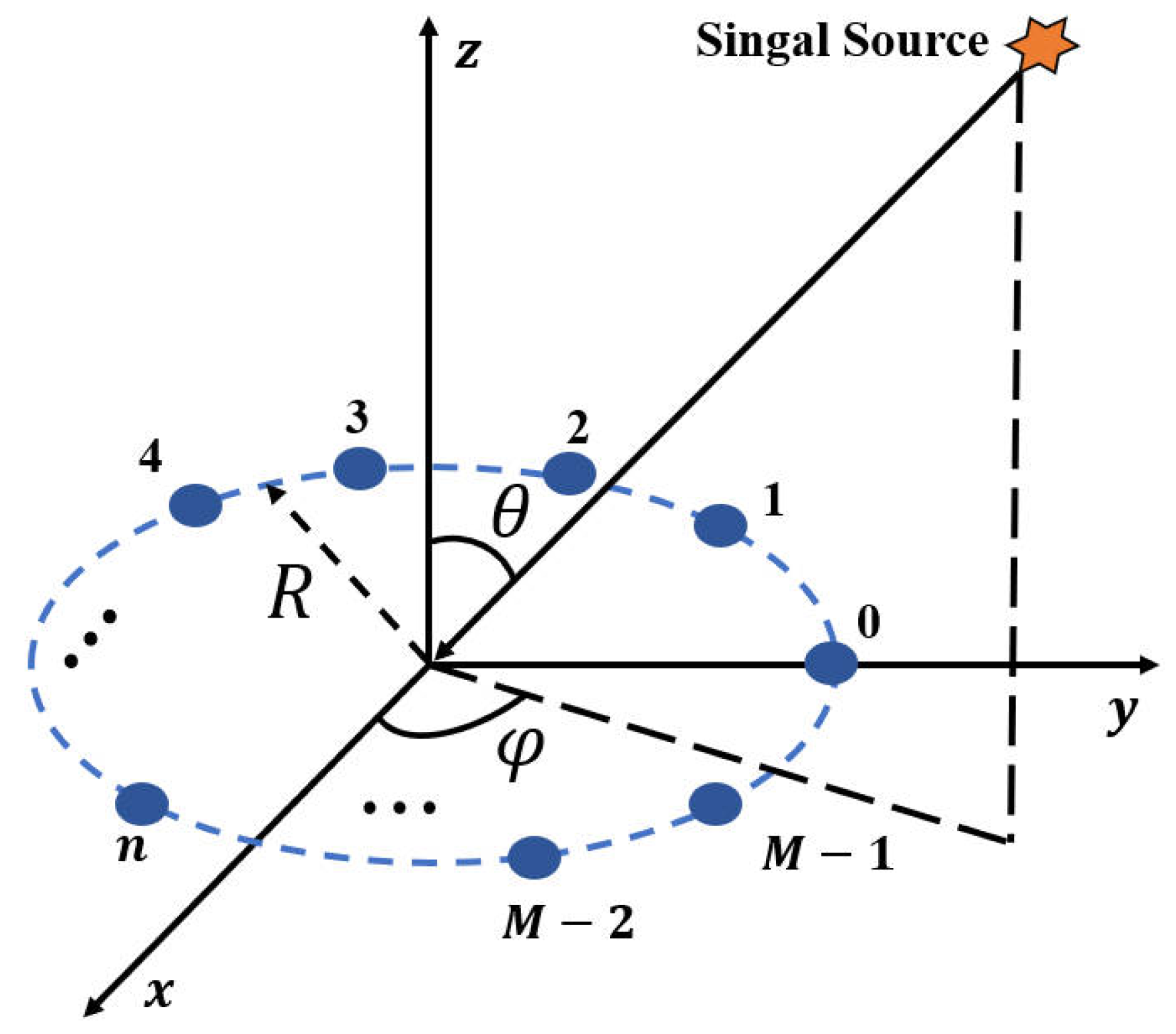
Figure 2.
Flowchart of the WAA algorithm.
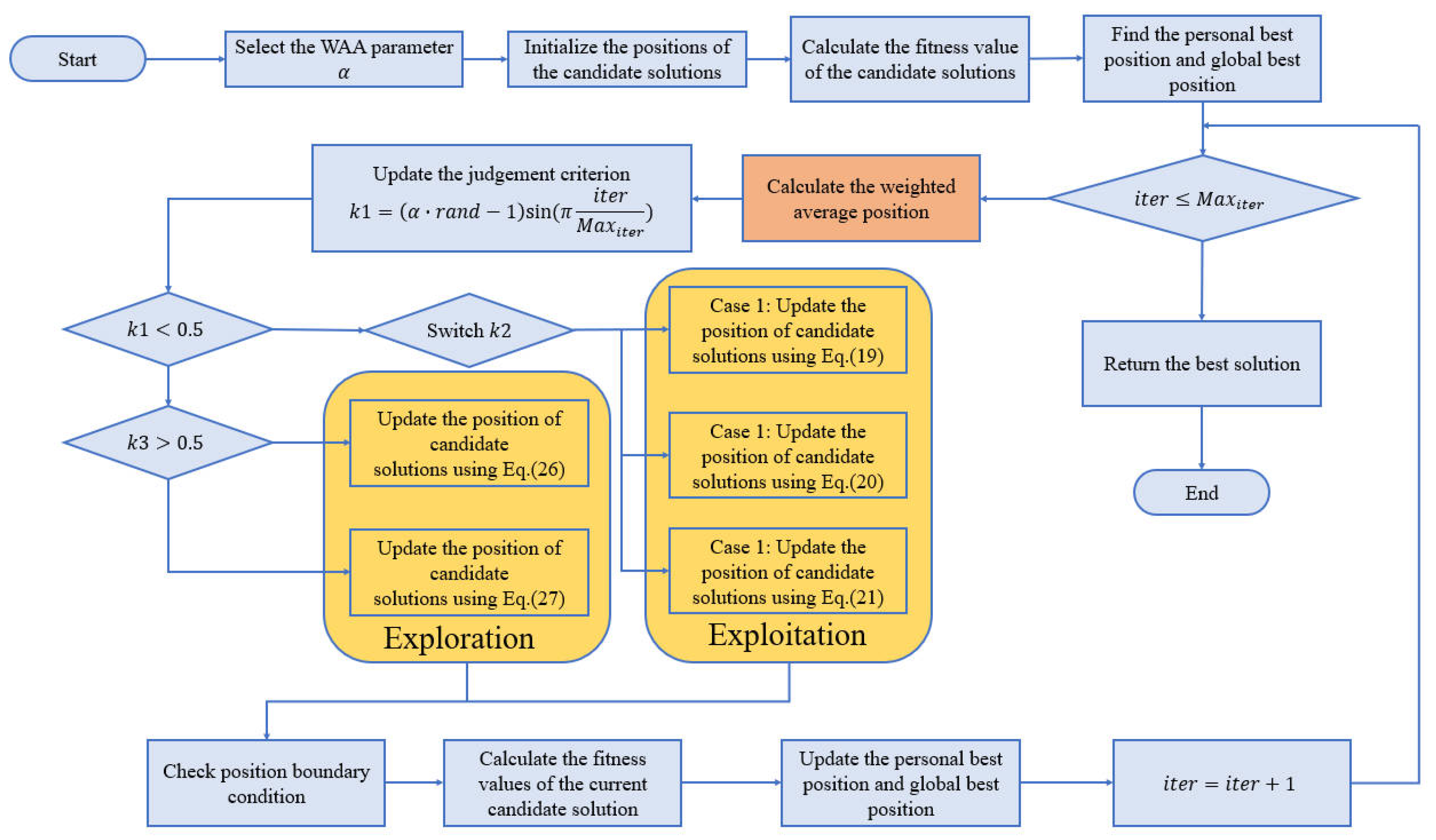
Figure 3.
Comparison of optimal fitness curves across different optimization algorithms.
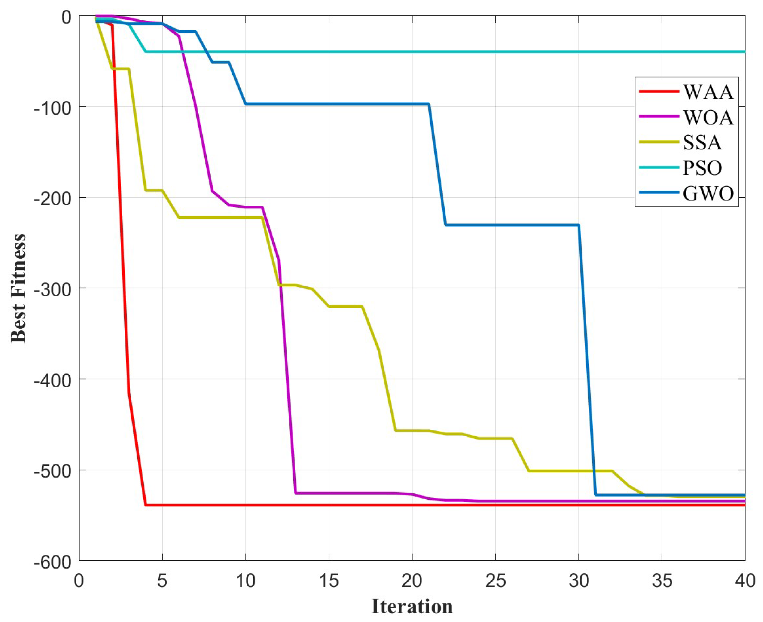
Figure 4.
Block diagram of the DF system.
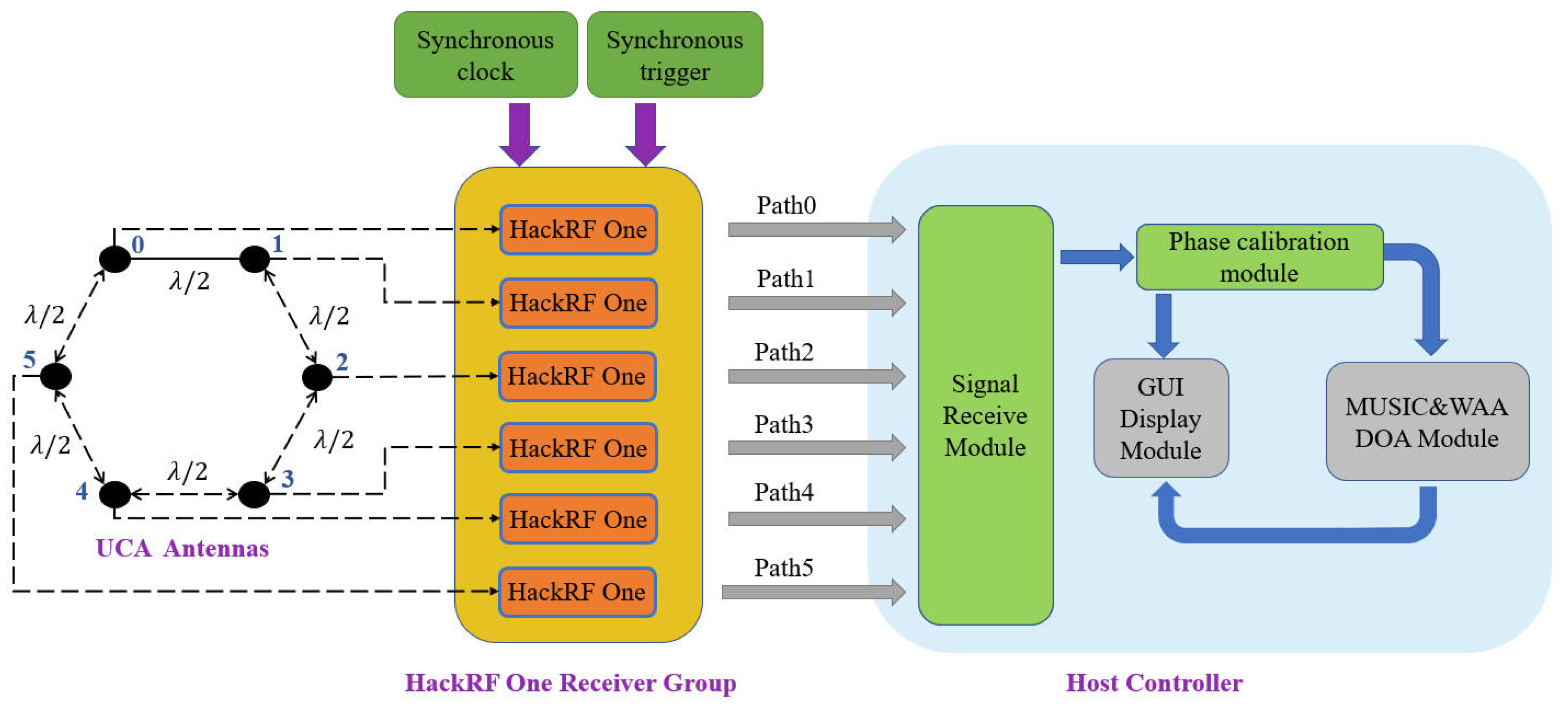
Figure 5.
Physical components of the DF system.
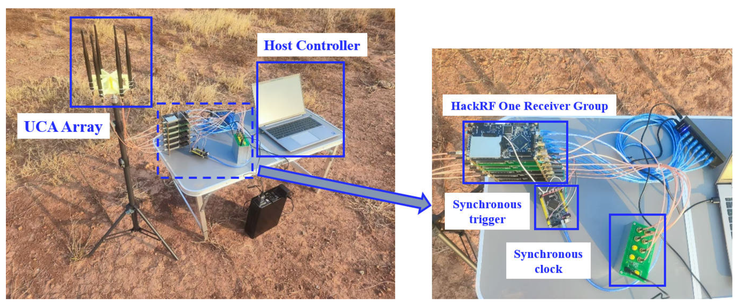
Figure 6.
Calibration process of the DF system.
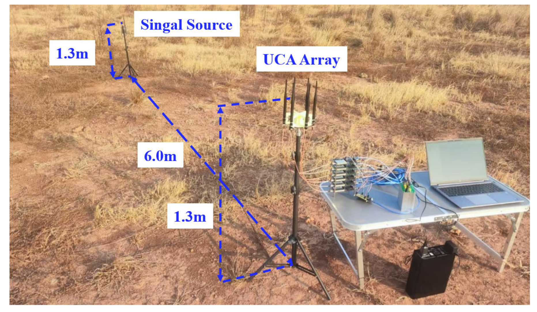
Figure 7.
Experimental scene with the DJI AIR 2S UAV.
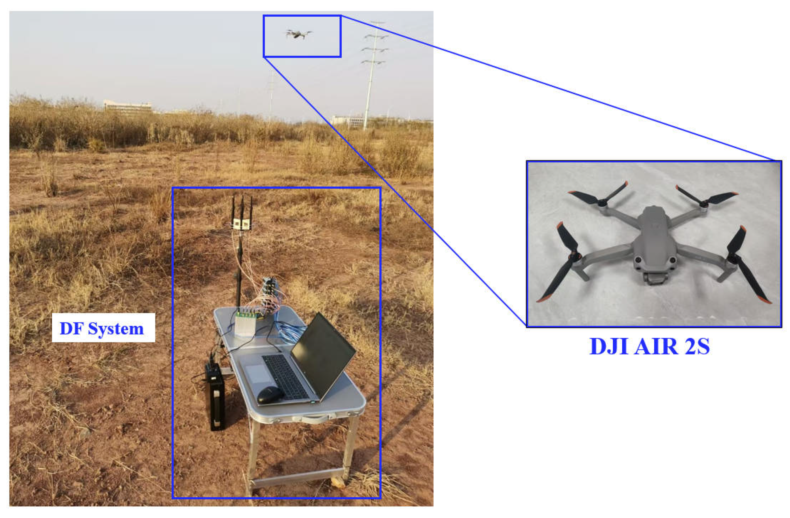
Figure 8.
Rf signal characteristics of the UAV.
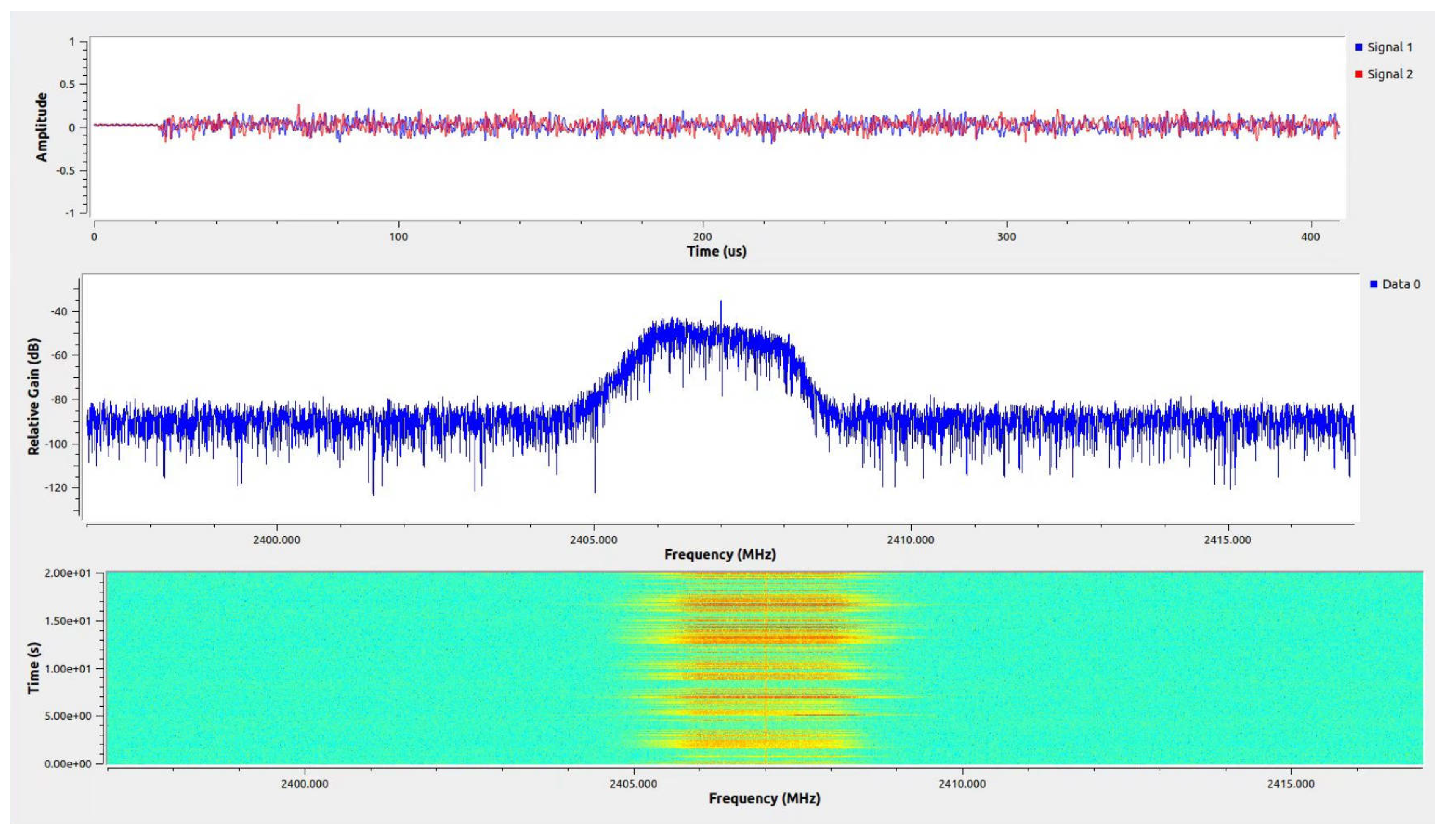
Figure 9.
Two UAV flight trace paths.
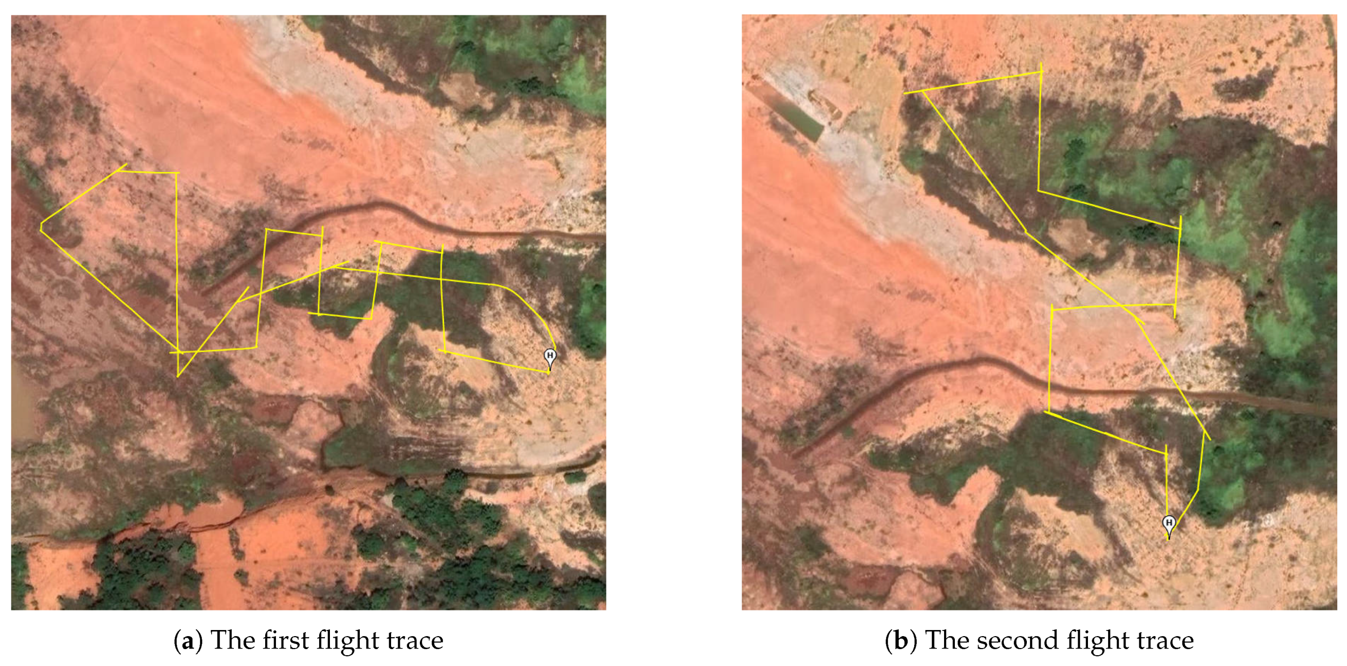
Figure 10.
Rf signal characteristics of the UAV.
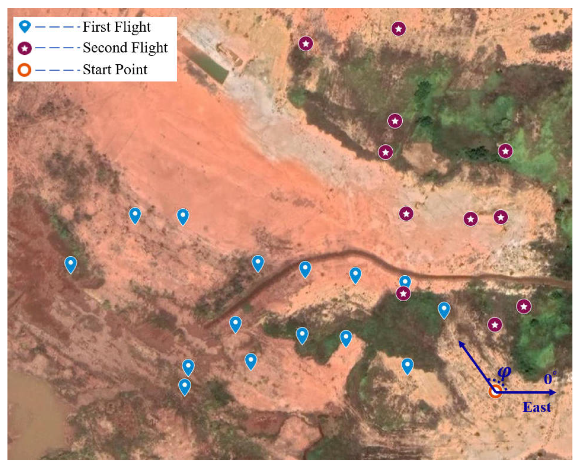
Figure 11.
The comparison between measured and calculated value of azimuth and elevation
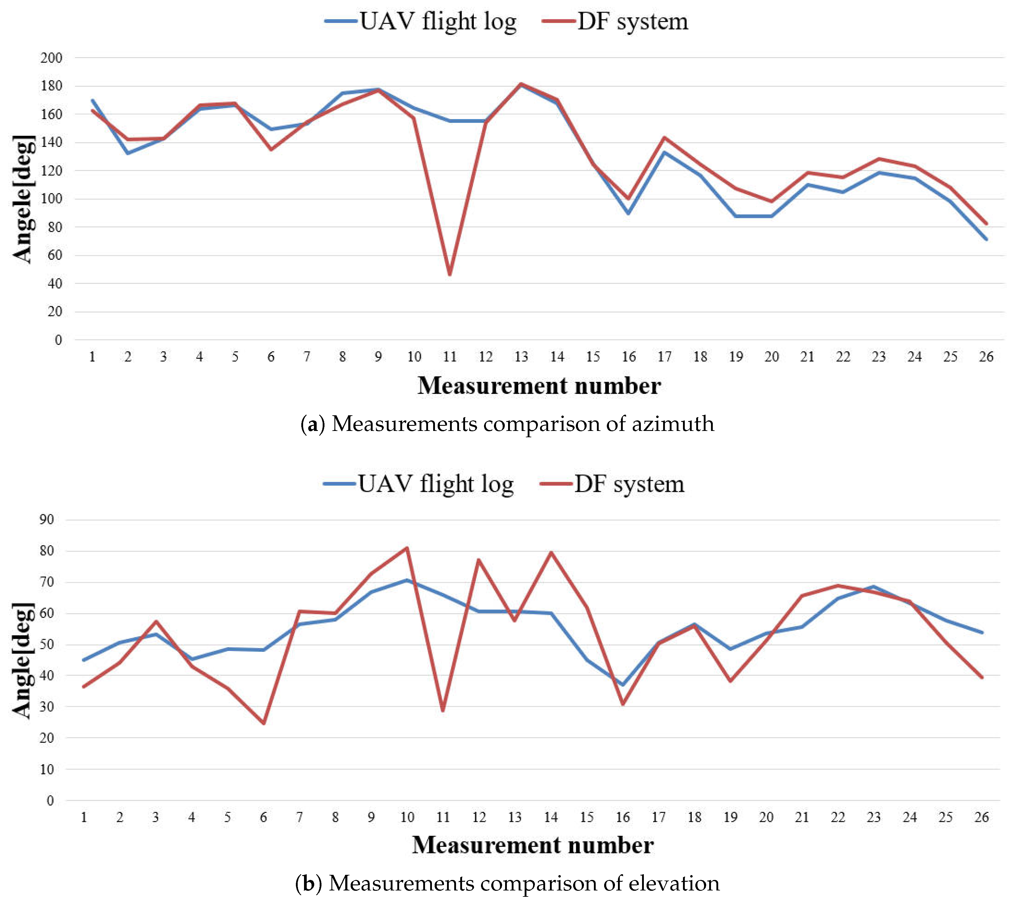
Figure 12.
Comparison of real-time azimuth angle measurements from two flight experiments with the corresponding values from the UAV flight log.
Figure 12.
Comparison of real-time azimuth angle measurements from two flight experiments with the corresponding values from the UAV flight log.
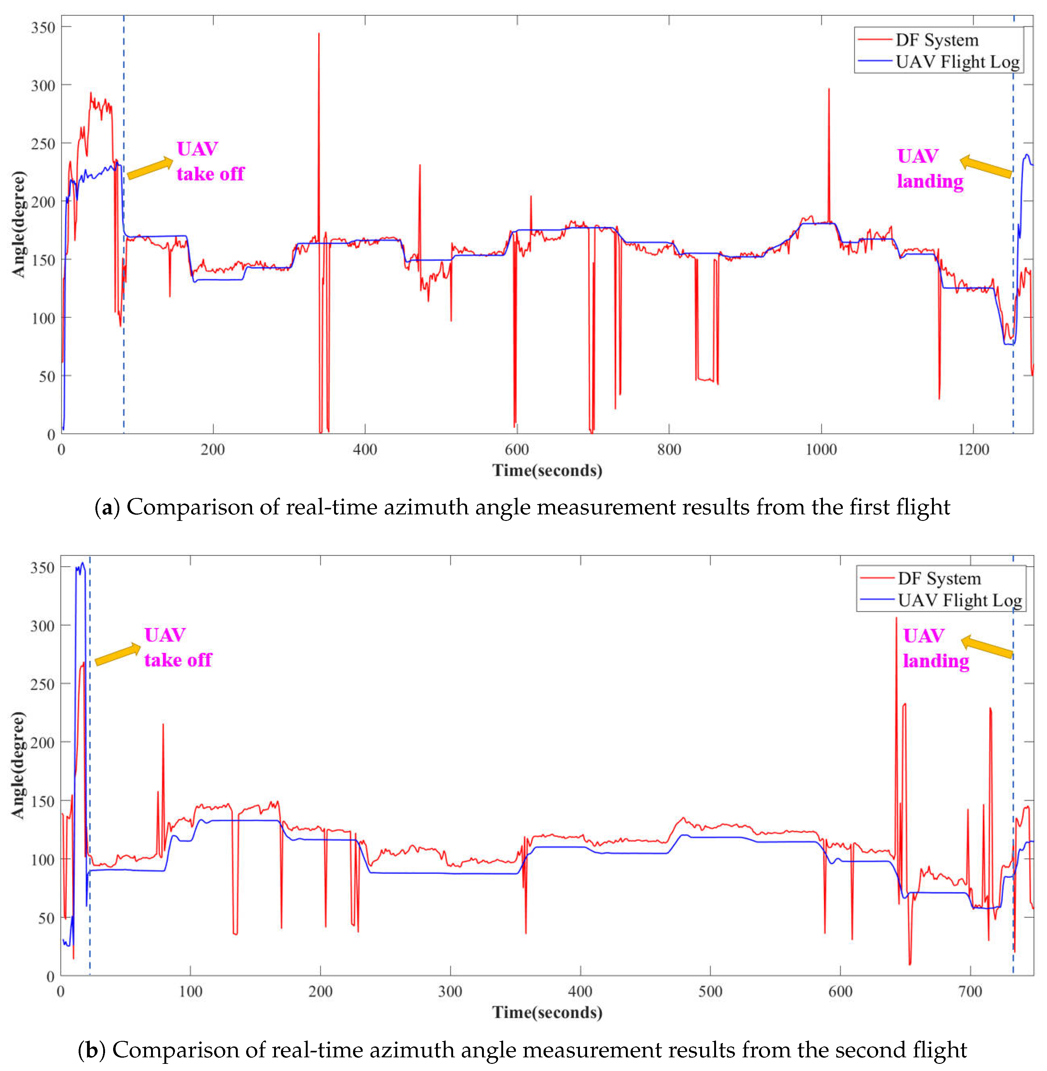
Figure 13.
Comparison of real-time elevation angle measurements from two flight experiments with the corresponding values from the UAV flight log.
Figure 13.
Comparison of real-time elevation angle measurements from two flight experiments with the corresponding values from the UAV flight log.
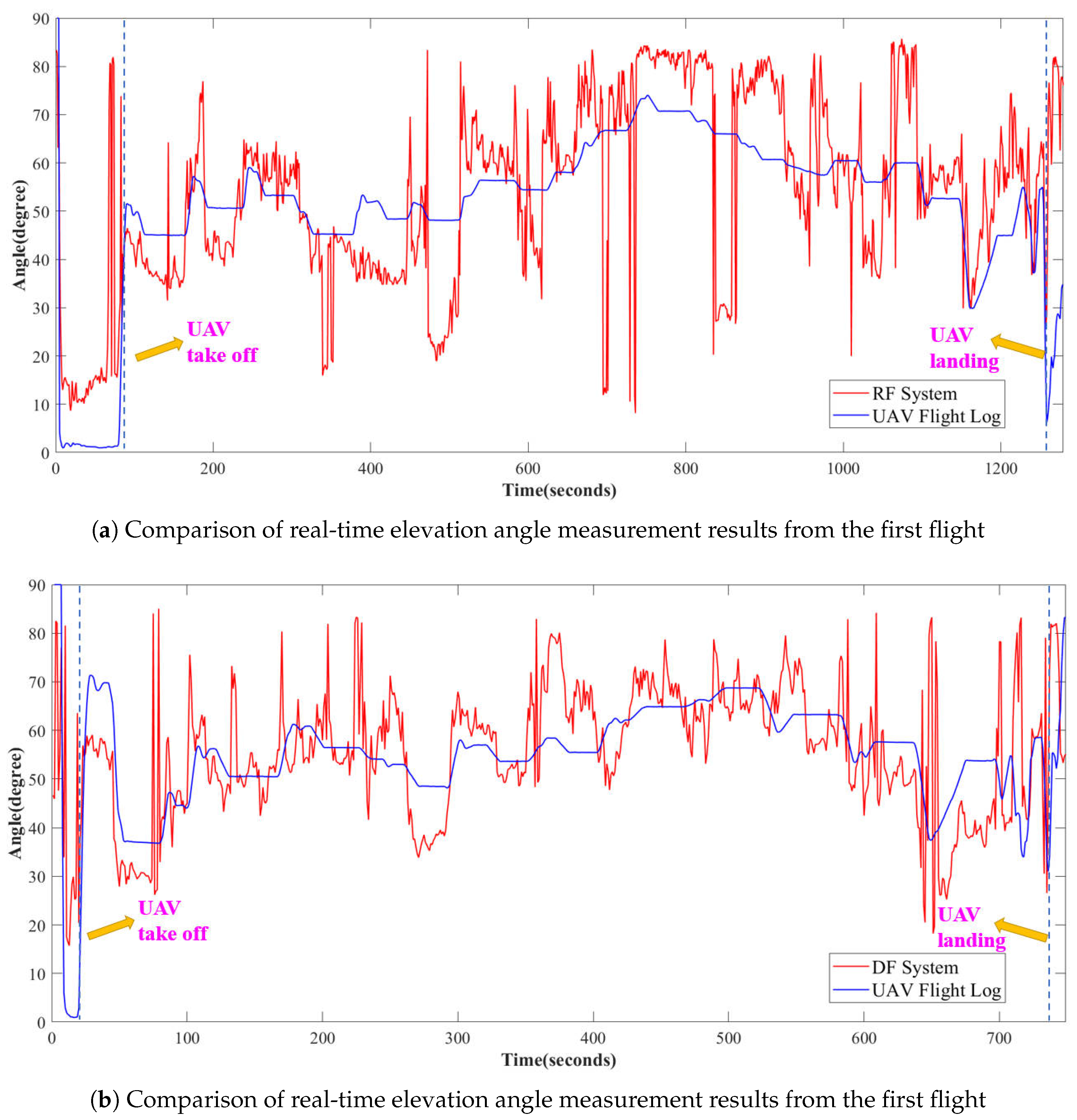
Table 1.
Distance and height of UAV hovering points.
| Index | Latitude | Longitude | Altitude(m) | Distance(m) | Height(m) |
|---|---|---|---|---|---|
| 0 (start) | 25.76984011 | 114.7491364 | 140.4 | 0.0 | 0.0 |
| 1 | 25.76990561 | 114.7487381 | 180.8 | 40.6 | 40.4 |
| 2 | 25.77024192 | 114.7487277 | 189.8 | 60.5 | 49.4 |
| 3 | 25.77027657 | 114.7485007 | 200.1 | 80.0 | 59.7 |
| 4 | 25.77001880 | 114.7484583 | 210.6 | 70.8 | 70.2 |
| 5 | 25.77002978 | 114.7482601 | 220.7 | 90.3 | 80.3 |
| 6 | 25.77030159 | 114.7482745 | 230.4 | 100.4 | 90.0 |
| 7 | 25.77032455 | 114.7480587 | 220.5 | 120.6 | 80.1 |
| 8 | 25.76992283 | 114.7480253 | 210.0 | 111.7 | 69.6 |
| 9 | 25.76990013 | 114.7477439 | 200.5 | 139.7 | 60.1 |
| 10 | 25.77032015 | 114.7472073 | 210.5 | 200.5 | 70.1 |
| 11 | 25.77051998 | 114.7474993 | 220.7 | 180.5 | 80.3 |
| 12 | 25.77051499 | 114.7477191 | 230.4 | 160.5 | 90.0 |
| 13 | 25.76982094 | 114.7477251 | 220.5 | 141.5 | 80.1 |
| 14 | 25.77007673 | 114.7479557 | 210.4 | 121.2 | 70.0 |
| 15 | 25.77013401 | 114.7489039 | 180.5 | 40.0 | 40.1 |
| 16 | 25.77011233 | 114.7491332 | 180.4 | 30.2 | 40.0 |
| 17 | 25.77024124 | 114.7487190 | 190.6 | 60.9 | 50.2 |
| 18 | 25.77056632 | 114.7487316 | 200.1 | 90.1 | 59.7 |
| 19 | 25.77055245 | 114.7491622 | 210.3 | 79.1 | 69.9 |
| 20 | 25.77082168 | 114.7491817 | 220.7 | 109.0 | 80.3 |
| 21 | 25.77094563 | 114.7486809 | 230.3 | 130.7 | 89.9 |
| 22 | 25.77132218 | 114.7486960 | 220.2 | 170.0 | 79.8 |
| 23 | 25.77126209 | 114.7482753 | 220.1 | 179.6 | 79.7 |
| 24 | 25.77081717 | 114.7486373 | 200.4 | 119.2 | 60.0 |
| 25 | 25.77054422 | 114.7490243 | 190.4 | 78.9 | 50.0 |
| 26 | 25.77018674 | 114.7492656 | 170.1 | 40.7 | 29.7 |
Disclaimer/Publisher’s Note: The statements, opinions and data contained in all publications are solely those of the individual author(s) and contributor(s) and not of MDPI and/or the editor(s). MDPI and/or the editor(s) disclaim responsibility for any injury to people or property resulting from any ideas, methods, instructions or products referred to in the content. |
© 2025 by the authors. Licensee MDPI, Basel, Switzerland. This article is an open access article distributed under the terms and conditions of the Creative Commons Attribution (CC BY) license (http://creativecommons.org/licenses/by/4.0/).
Copyright: This open access article is published under a Creative Commons CC BY 4.0 license, which permit the free download, distribution, and reuse, provided that the author and preprint are cited in any reuse.


