
Submitted:
11 April 2025
Posted:
14 April 2025
You are already at the latest version
Abstract
New positioning solutions are a key factor in the pursuit of autonomous driving. GNSS is the most common method, however traditional systems may have high position errors due to multipath signals. In this work, we present a GNSS adaptive antenna with beamforming capabilities that can apply spatial filtering to mitigate interferences and improve satellite connectivity, reducing the positioning error. The array, developed with off-the-shelf GNSS antennas, was used to demonstrate the improvement of the gain, leading to better signal to noise ratio, comparatively to the traditional GNSS antenna, while maintaining circular polarization in all directions. A digital beamforming solution was employed with the software defined platform based on a Xilinx ZCU216. The full system performance was tested in an anechoic chamber, where good results were obtained in both single and multibeam scenarios, with great agreement between the simulated and measured data. The results presented in this paper validate the proposed FPGA-based array and beamforming development platform, paving the way for the seamless and rapid design and test of numerous antenna array geometries with up to 16 channels and beamforming algorithms, including adaptive ones. This powerful and versatile tool will accelerate research on performance improvement of GNSS reception.
Keywords:
GNSS
; FPGA
; digital beamforming
; antenna array
1. Introduction
New solutions for navigation and positioning are deemed essential for autonomous driving applications [1]. GNSS is the most common tool for this endeavor, however the position error of modern systems ranges the 30 centimeters in best case scenarios [2], not reaching the under 10 cm errors requirements for fully-autonomous driving [3]. Depending on the environment, it may be difficult to evaluate the position due to signal degradation, blockage or interference [4]. The antenna is a key component of positioning systems, but traditional antennas are static, which means they cannot adapt to the surrounding environment, which can be very dynamic (e.g., a car travelling through a city where multipath signals are abundant) [4]. While multipath signals are an interference that happens due to the interaction between GNSS signals and the environment, there are also man-made interferences that can intentionally disable or trick the GNSS positioner. These interferences are called jamming and spoofing. Jamming consists in broadcasting signals with the same characteristics as GNSS satellite signals, but at much higher power levels, degrading the carrier to noise ratio of the GNSS signals and making it impossible for the GNSS receiver to acquire them. On the other hand, spoofing consists in generating fake GNSS signals with navigation data that is interpreted by the GNSS receiver and tricking it into generating an erroneous positioning and timing solution without awareness [5]. As it becomes apparent, for fully autonomous driving solutions to be safe and reliable, it is of paramount importance to grant positioning systems with resilience against these interferences.
Considering that, usually, satellite signals come predominantly from above the antenna (zenith) and that multipath signals and man-made interferences usually have low elevation angles (horizon), choke ring antennas have been proposed as solutions to this issue [6,7]. However, these antennas are static and cannot adapt to a highly dynamic environment such as the ones where autonomous vehicles will need to operate. Additionally, if the interferences are placed at higher elevation angles (such as the top of a tall building), then the efficacy of the choke ring antenna on ignoring these signals is compromised.
With the use of an antenna array, it is possible to dynamically adjust the radiation characteristics of the antenna, allowing for spatial filtering of the received GNSS signals by attenuating the multipath signals and increasing the gain of direct satellite signals [8]. Furthermore, it is also possible to identify the Direction of Arrival (DoA) of jamming or spoofing signals and dynamically mitigate them through spatial filtering [5].
The implementation of an antenna array is not, however, as straightforward task. The increased number of antennas that compose the array occupies a large area and requires a complex feeding network. A beamforming mechanism is also necessary, which can be performed in the analog or digital domain. In the analog domain, the phase and amplitude are implemented by individual circuitry channels for each antenna element. Then, these signals can be individually sampled by multiple Analog-to-Digital Converter (ADC), or merged to be simultaneously sampled by a single ADC. As for the digital domain, the beamforming is performed at the digital level, allowing to reduce component count and providing greater control over the phase delay between feedlines, at the expense of higher computation cost [9]. However, every antenna must be directly connected to an ADC, which must be able to sample synchronized signals, at high sampling frequency, requiring ADCs that are usually expensive, making the overall system costly and complex [10].
The use of antenna arrays for GNSS multipath and interference mitigation has been attempted and reported in literature, with the solution based on 4 antenna planar arrays being the most prominent design reported. In [11] the authors use a 2x2 planar array composed of E1/E5 dual-band patch antennas placed just under λ0/2 from each other to demonstrate mitigation of jamming and spoofing signals in realistic scenarios with good results. Similarly, in [12] a 190x190 mm 2x2 planar array composed of commercial off-the-shelf (COTS) patch antennas at λ0/2 spacing was used as part of a system for multipath detection. Resorting to a software defined radio (SDR), the MUSIC algorithm was implemented and, with beamforming, an increase of C/N0 of up to 8 dB was achieved. In [13], a 4 element half-wavelength circular array was used in combination with COTS GNSS receiver and FPGA to evaluate nulling capabilities for intentional interference mitigation. A field test demonstrated that up to two sources of interference could be countered while maintaining sufficient carrier to noise ratio for the GNSS receiver. In [14] a 140x140 mm2 planar 2x2 array of patch antennas with d=λ0/3 was presented. Different designs can also be found, with a 1x4 linear array of custom-made patch antennas being presented in [15]. Each patch is 40.9x40.9 mm2 (0.21λ0 x0.21λ0) and the center-to-center distance in the array is 66 mm, around 0.35λ0 at 1.57542 GHz. The array was controlled by a hardware beamformer and its beamforming was demonstrated. Being a linear array, the beamforming capabilities were limited from design and mutual coupling compensation was not considered, which was a considerable design flaw given the close distance between antenna elements in the array. In [16] a circular array of 7 dual-band (L1/L2) antennas was reported. The array had a diameter of 500 mm and the antennas are spaced by 125 mm. The array was tested for its nulling capabilities with both hardware and software beamforming systems.
The reported arrays are mostly composed of 4 antennas, since the complexity of the hardware and software required for more antennas will increase rapidly with the number of antennas. In this work, we will present a 16 antenna (4x4 planar array) solution developed resorting to a powerful FPGA-based array and beamforming development platform (ABDP), designed to expedite the development of arrays and beamforming algorithms [17]. This approach allows to re-use a reconfigurable platform, making it easier to adapt the control electronics to the antenna size.
At this stage of development, an off-the-shelf antenna element was used to operate on/in? the L1/E1 band (1.57542 GHz). The array must be designed to be integrated into a car’s rooftop, without significantly changing its appearance, therefore the system must have a small footprint and be as thin as possible. Additionally, the system must be compatible with standard GNSS receivers, therefore its output signal must be compatible to what is expected from a single antenna that is fed to the receiver, for correlation and tracking. The performance will be evaluated under interference constraints, while directing the main beam to different directions, and the evaluation of the system’s capabilities to perform multibeam beamforming to track multiple satellites simultaneously. The design and simulation the antenna array for GNSS applications will be presented (section 2), and the beamforming mechanism employed in the ABDP, implemented in the ZCU216 FPGA, is described (section 3). Finally, the array and the ABDP are integrated, and the system’s full performance is evaluated in an anechoic chamber (section 4).
2. Antenna Array Design
To build the antenna array, we start by analyzing the performance of an off-the-shelf (COTS) antenna. The ceramic antenna is a low-cost, low form factor passive patch antenna commercialized for GNSS applications. Owing to these attributes, along with its performance, the adequate datasheet and 3D models that the manufacturer provides for this antenna, it was selected as the commercial antenna to consider for the design of the array. Simulations are performed with a full-wave solver is utilized, in this case CST (Computer Simulation Technology) studio suite by Simulia.
2.1. Modelling of COTS GNSS Antenna
The first step after picking the antenna was to draw the antenna in CST using both the 3D CAD model and the technical drawing available online. The antenna is composed of five main structures (Figure 1). The position of the antenna in the ground plane was chosen to be the best location specified in the datasheet by the manufacturer and corresponds to the center of the 70x70x1.5 mm3 ground plane. To simulate real testing, a coaxial connector was also added, and the feed port is placed at the end of the connector. The Z axis of the coordinate system (θ = 0˚) is perpendicular to the patch’s surface. The dimensions and materials available in the datasheet/CAD were used. In Table 1, are summarized the antenna parameters, their value, and assigned CST materials.
In case of the dielectric, the manufacturer only specifies that it is a ceramic. Therefore, a sweep of the dielectric constant, εr, was performed to match both the S11 and axial ratio presented in the datasheet. Figure 2 shows that a good agreement was obtained with εr = 20.65, and therefore this was the value adopted for the antenna array simulations.
The axial ratio (AR) at 1.57542 GHz in the elevation plane for φ = 0˚ and φ = 90˚ are presented in Figure 3. In both planes, the axial ratio is slightly above 3 dB, the desired axial ratio upper limit for circular polarized antennas on the radiating side of the patch. Although, from Figure 2, the AR is shown to be below 3 dB, that’s only marginally around the frequency of 1.57 GHz, and not at 1.57542 GHz. Note that these results were obtained from the approximated value of εr, meaning that they can be slightly off from the actual values.
In Figure 4, the simulated realized gain patterns for LHCP and RHCP are presented in both φ = 0˚ and φ = 90˚ directions. In both directions, the maximum realized gain is -2.95 dBi for LHCP signals (-8.9 dBi if we consider only the top side of the patch). As for the RHCP, the maximum realized gain is 5.15 dBi, which agrees with the datasheet’s stated 5.5 dBi gain. Once again, this behavior shows the RHCP affinity of the antenna.
Finally, the antenna apparent phase center was estimated to be at (0.22, 1.70 , 1.32) mm, very close to the geometric center of the antenna, which is the reference point (0, 0, 0). To understand the phase center variation, the plots for both φ = 0˚ and φ = 90˚ elevation plane phase for LHCP and RHCP are presented in Figure 5. In the case of RHCP, in the plane φ = 0˚ the phase varies 5.23º˚ and in the plane φ = 90˚ varies 0.68º˚, for θ between -90˚ and 90˚. These results show that the antenna has a small phase center variation (PCV).
This antenna showed good performance in most of its characterized parameters. The antenna can mitigate LHCP with low gains when compared to RHCP signals and even has low variation in the phase center, which is important for GNSS applications.
2.2. Array Geometry
In this section, the geometry of the antenna array will be discussed, where three key deign parameters were considered. First, the gain and half power beam width (HPBW) of the array, which changes proportionally with the number of antennas. Second, the complexity of a future analog or digital beamforming system, as the number of required components, computational power and cost also increases with the number of antennas in the array. Third, the size of the array increases as more antennas are used. With this mind, a 16-antenna square array was proposed, as it is a good compromise of the three previous figures, along with the square being the most common array geometry.
The distance between elements was chosen to keep the array as small as possible, keeping in mind the limited space availability in the car, without significantly hindering performance and considering the effect of mutual coupling. For all the accounted combinations of element spacing and array geometry that use 16 antennas, the array factor (AF) was analyzed for broadside, endfire, and in-between configurations using Matlab’s Sensor Array Analyzer toolbox.
Since the objective of the work was the development of an antenna array for GNSS signal spatial filtering, high directivity of the AF and low HPBW must be achieved. Analyzing the data concerning square arrays with different element spacing of 0.33λ0, 0.4λ0, 0.5λ0 and 0.75λ0, it was possible to verify that, as expected, the main lobe directivity increases as the distance d between the array elements increases. On the other hand, the half power beamwidth decreases. Given this, it would seem intuitive that, since the goal is to obtain high directivity and low HPBW, d should be as high as possible. However, higher values lead to more and higher grating lobes: as detailed in [18], side lobes are small compared to the main beam when the following criteria is met:
Because the intention is to direct the main beam to values of θ ranging from 0˚ to 90˚, from horizon to zenith, ideally should be less than in order to reduce the grating lobe levels, coinciding with the following statement from Balanis [19]: “to have only one end-fire maximum and to avoid any grating lobes, the maximum spacing between elements should be less than ”.
A compromise between the directivity and HPBW of the array with d = 0.5λ0 and the low grating lobe level achieved with d = 0.33λ0 is achieved with d = 0.4λ0.
2.3. Array Simulation
The antenna array was designed in CST resorting to the Array Task tool and it was studied with its main beam pointing towards the following set of φ and θ angles: (0,0), (0, 45), (0,90), (45, 45), (45, 90), (90, 45), (90, 90). This selection of directions allows the study of the array’s characteristics and performance when pointing to the zenith (broadside) and to the horizon (endfire) in two orthogonal planes, and with a step in-between. As the antennas in the array are symmetrically positioned, the performance in this 90˚ segment of the array is representative of the array’s performance in the remaining directions.
The 3D model of the square array of d=0.4λ0 and size of 305x305 mm2 is presented in Figure 6. The ground plane of each antenna element was extended so it is a single structure common to all antennas.
The simulated 3D radiation patterns of the square array pointing to the previously enumerated directions are presented in Figure 7, and the 2D plots in the elevation plane cut are presented in Figure 8. As it can be seen, the gain is highest in the broadside direction (14.9 dBi), as expected, since both the antenna element gain and the array factor’s directivity are highest in this direction. When θ = 45˚, the gain is slightly lower (13.3 dBi for φ = 0˚), as both the antenna element gain and the array factor directivity are lower at this angle. This fact is also the reason why the array is not capable of adequately pointing the beam towards θ = 90˚: the antenna element has much lower gain towards the horizon, thus hindering the array’s performance in this plane. However, the array is still capable of achieving a gain of 6.2 dBi for φ = 0˚ and θ = 90˚ and 5.2 dB for φ = 90˚ and θ = 90˚ while the single antenna element can only provide a gain of -3.4 dBi and -3.0 dBi, respectively, thus accomplishing the goal of improving signal reception at low elevations.
Figure 9 presents the axial ratio of the array when the main beam is directed towards the aforementioned directions. It is possible to observe that the array maintains reasonable circular polarization (AR close to 3 dB) in the directions at which the main beam points to. This statement holds true even for beam directions of θ = 90˚, except for the case where φ = 0˚, where the AR at the 90˚ mark is over 10 dB. This could be due to the inherent asymmetry of the antenna element on the square array and it is a possible path to be explored in future work.
3. Beamforming System
Beamformers can be divided into their analog and digital counterparts [20,21]. Analog beamformers modify phase and gain through phase shifters and variable gain amplifiers, while digital beamformers change them by multiplying the sampled signals by complex weights. However, the control platform used is very similar to both. Both require a control platform used to calculate the phases or complex weights usually using very similar algorithms. In this work, we employed the ABDP platform [17] to test digital beamforming approaches resorting to a Zynq UltraScale+ RFSoC ZCU216 evaluation board from Xilinx, which utilizes the XCZU49DR RFSoC.
The block diagram of the proposed system is presented in Figure 10, and it is composed of 4 major components: the ADCs, the Processing System (which includes the beamforming algorithm), the Programmable Logic and the DAC.
The digital samples from each antenna’s signal acquired by the ADCs are supplied to the programmable logic (PL) via the PL interface, where weights calculated by the beamforming algorithm are applied to the samples. The output of the PL contains the improved signal containing information of every satellite. Before converting the signal back to its analog form, the signal must be mo
dulated back to the 1.57542 GHz frequency. The result is a similar signal to the one sampled, but now with improved satellite signal quality. It can then be converted to its analog form using the DAC. This analog output is then able be supplied to a traditional GNSS receiver.
3.1. Beamforming Algorithm
To access the antenna array capabilities, a simple beamforming algorithm was implemented. This beamforming algorithm points the main lobe to the user specified elevation, θ0, and azimuth, ϕ0, angles. The following phases between elements are evaluated using the reference frame in Figure 11. Here βx and βy are the phase between elements, dx and dy the distance between elements in the x and y direction, respectively, and λ is the wavelength of the signals.
The effective phase for each element βmn is the accumulative sum of both βx and βy for the element position [22]:
where m and n are the positions of the nth element in the x and y directions, respectively. The phase on each element is then converted to the complex phase delay notation to be multiplied with the incoming signal from each antenna [22]:
where and are the incoming and phase shifted complex signals from the antenna element in the nth position, respectively. Finally, the delayed signals are summed, resulting in the beamformed signal.
4. Measurement Results and Performance Analysis
The antenna array was integrated into the ABDP for testing of the full system in an anechoic chamber. Each of the antennas was connected to an ADC channel, and the system was placed in the anechoic chamber as demonstrated in Figure 12, with the antenna array mounted on a foam platform facing the transmission antenna (Q-Par Angus WBH2-18S) and the ABDP being covered in panels that absorb RF waves.
The azimuth plane radiation patterns of the array were first obtained for four directions at 2 different planes. The planes tested were φ = 0˚and φ = 45 ˚ , where the main beam was pointed towards θ = 0˚ (broadside), θ = 340˚, θ = 60˚ and θ = 300˚. The same radiation pattern was simulated in CST, and the results are presented in Figure 13 and Figure 14.
There is a great agreement between measured and simulated patterns. In terms of the main lobes, it was possible to point the beam to the desired positions, with the noticeable deviation at higher θ values such as in the θ =60˚ and θ = 300˚, which was expected as discussed previously. Nevertheless, the measurements and the simulations present the same limitations of the system. There is a slight difference in the sidelobes and the nulls between the two planes, that is, in the φ = 45˚ plane there are slight larger null and sidelobe relative to the simulations. This can be due to mutual coupling between antenna elements that is not reproduced by the simulations due to material imperfections, or small misalignments in the measurement setup and the array itself. It is not possible to compare the absolute gain values of the measurement with the simulation because the analog signal measured by the VNA is generated by the DAC of the ZCU216, as previously discussed. Moreover, these results are normalized to the value at φ = 0˚ and θ = 0˚, separately for the two planes.
In addition to the single beam tests, a multibeam radiation pattern was also simulated and measured. The three beams were pointed towards θ = 0˚, θ = 45˚ and θ = 330˚. The azimuth plane radiation patterns are presented in Figure 15. It is possible to observe that the proposed system successfully produced a radiation pattern with the three proposed beams. The measured multibeam radiation pattern greatly matches the predicted one. As it can be seen, maxima could be pointed towards the desired θ = 0˚ and θ = 45˚ directions, while the beam towards θ = 330˚ was slightly shifted towards θ = 315˚. Since this was predicted by the simulation, it is possible to conclude that it is due to the array’s resolution limitation. This could potentially be improved with the use of arrays with more elements. In the direction of the θ = 330˚, it is visible that the measure gain deviates slightly from the theoretical value. This can be explained by the measurement setup demonstrated in Figure 12. When pointing towards θ = 330˚, the array starts to turn towards the box containing the ABDP and the cables, which interferes with the ideally-anechoic environment of the anechoic chamber, leading to a reduction in the received power.
5. Conclusion and Future Work
In this work, a GNSS adaptive antenna array with digital beamforming was reported. The array was developed with COTS GNSS antennas. The performance of these antennas was validated via simulation in CST. The array geometry was studied resorting to Matlab, and the final array simulations were performed in CST. It was demonstrated that the proposed array is capable of improving the gain comparatively to the traditional GNSS antenna in all directions, even close to the horizon. It was also possible to observe that the array maintains reasonable circular polarization in the directions at which the main beam points to.
A digital beamforming solution was developed in Xilinx’s ZCU216, with each of the array’s 16 antennas being connected to an ADC channel. The GNSS signals, after being sampled by the ADCs, were weighed according to a beamforming algorithm which received as inputs the direction towards which the main beam was to be pointed. The full system was tested in an anechoic chamber, where good results were obtained in both single and multibeam scenarios, with a great agreement between the simulated and measured data.
Nevertheless, desirable improvements in the system have been identified, namely the use of custom GNSS antennas with better AR over the range of interest. Furthermore, it was verified that in the multibeam approach, the results could be improved by developing an array with an improved HPBW, either by using more directive antenna elements or by geometry redesign.
The results presented in this paper validate the FPGA-based array and beamforming development platform, paving the way for the seamless and rapid design and test of numerous antenna array geometries with up to 16 channels and beamforming algorithms, including adaptive ones. This powerful and versatile tool will accelerate research on performance improvement of GNSS reception.
Author Contributions
Conceptualization, G.D., H.D., D.B. and P.M.M.; methodology, G.D., H.D., D.B., and P.M.M.; software, G.D. and D.B.; validation, H.D. and P.M.M.; formal analysis, G.D., H.D., D.B.; investigation, G.D., H.D. and D.B.; resources, D.B. and P.M.M.; data curation, H.D. and D.B.; writing—original draft preparation, G.D., H.D., and D.B.; writing—review and editing, G.D., H.D., D.B. and P.M.M.; supervision, H.D. and P.M.M.; project administration, H.D., D.B. and P.M.M.; funding acquisition, P.M.M. All authors have read and agreed to the published version of the manuscript.
Funding
This work is supported by national funds, through the Operational Competitiveness and Internationalization Programme (COMPETE 2020) [Project nº 179491; Funding Reference: SIFN-01 9999-FN-179491].
Data Availability Statement
The raw data supporting the conclusions of this article will be made available by the authors on request.
Conflicts of Interest
Author Diogo Baptista was employed by the company Bosch Car Multimedia Portugal, S.A. The remaining authors declare that the research was conducted in the absence of any commercial or financial relationships that could be construed as a potential conflict of interest.
References
- L. Chen, F. Zheng, X. Gong, and X. Jiang, “GNSS High-Precision Augmentation for Autonomous Vehicles: Requirements, Solution, and Technical Challenges,” Remote Sens (Basel), vol. 15, no. 6, p. 1623, Mar. 2023. [CrossRef]
- Y. Gu, L.-T. Hsu, and S. Kamijo, “GNSS/Onboard Inertial Sensor Integration With the Aid of 3-D Building Map for Lane-Level Vehicle Self-Localization in Urban Canyon,” IEEE Trans Veh Technol, vol. 65, no. 6, pp. 4274–4287, Jun. 2016. [CrossRef]
- T. G. R. Reid et al., “Localization Requirements for Autonomous Vehicles,” SAE International Journal of Connected and Automated Vehicles, vol. 2, no. 3, pp. 12-02-03–0012, Sep. 2019. [CrossRef]
- R. Sun, L. Fu, Q. Cheng, K.-W. Chiang, and W. Chen, “Resilient Pseudorange Error Prediction and Correction for GNSS Positioning in Urban Areas,” IEEE Internet Things J, vol. 10, no. 11, pp. 9979–9988, Jun. 2023. [CrossRef]
- Zhang, Cui, Xu, and Lu, “A Two-Stage Interference Suppression Scheme Based on Antenna Array for GNSS Jamming and Spoofing,” Sensors, vol. 19, no. 18, p. 3870, Sep. 2019. [CrossRef]
- Ł. Rykała et al., “Research on the Positioning Performance of GNSS with a Low-Cost Choke Ring Antenna,” Applied Sciences, vol. 13, no. 2, p. 1007, Jan. 2023. [CrossRef]
- S. Liu, D. Li, B. Li, and F. Wang, “A Compact High-Precision GNSS Antenna With a Miniaturized Choke Ring,” IEEE Antennas Wirel Propag Lett, vol. 16, pp. 2465–2468, 2017. [CrossRef]
- L. Huang, Z. Lu, Z. Xiao, C. Ren, J. Song, and B. Li, “Suppression of Jammer Multipath in GNSS Antenna Array Receiver,” Remote Sens (Basel), vol. 14, no. 2, p. 350, Jan. 2022. [CrossRef]
- Z. Peterson, “Types of Beamforming and Their Uses in RF PCBs.” Accessed: Jan. 12, 2023. [Online]. Available: https://www.nwengineeringllc.com/article/types-of-beamforming-and-their-uses-in-rf-pcbs.
- Microwave Journal, “Advantages/Disadvantages of Digital Beamforming in Satellite Applications.” Accessed: Feb. 15, 2023. [Online]. Available online: https://www.microwavejournal.com/blogs/28-apitech-insights/post/35492-advantagesdisadvantages-of-digital-beamforming-in-satellite-applications.
- M. Cuntz, A. Konovaltsev, and M. Meurer, “Concepts, Development, and Validation of Multiantenna GNSS Receivers for Resilient Navigation,” Proceedings of the IEEE, vol. 104, no. 6, pp. 1288–1301, Jun. 2016. [CrossRef]
- M. Razgūnas, S. Rudys, and R. Aleksiejūnas, “GNSS 2×2 antenna array with beamforming for multipath detection,” Advances in Space Research, vol. 71, no. 10, pp. 4142–4154, May 2023. [CrossRef]
- J. Arribas, C. Fernandez-Prades, M. A. Gomez Lopez, and T. R. Ruiz, “Receiver-independent GNSS Smart Antenna for Interference Mitigation,” in 2022 10th Workshop on Satellite Navigation Technology (NAVITEC), IEEE, Apr. 2022, pp. 1–8. [CrossRef]
- E. A. Marranghelli, R. L. La Valle, and P. A. Roncagliolo, “Simple and Effective GNSS Spatial Processing Using a Low-Cost Compact Antenna Array,” IEEE Trans Aerosp Electron Syst, vol. 57, no. 5, pp. 3479–3491, Oct. 2021. [CrossRef]
- X. Tang, Nasimuddin, X. Qing, and Z. N. Chen, “A circularly polarized beam-steering antenna system for GNSS applications,” in 2016 IEEE Region 10 Conference (TENCON), IEEE, Nov. 2016, pp. 1078–1081. [CrossRef]
- J. Curran, M. Bavaro, and J. Fortuny, “Analog and Digital Nulling Techniques for Multi-Element Antennas in GNSS Receivers,” Proceedings of the 28th International Technical Meeting of the Satellite Division of The Institute of Navigation, 2015.
- D. Gomes, D. Baptista, H. Dinis, P. M. Mendes, and S. Lopes, “Software-Defined Platform for Global Navigation Satellite System Antenna Array Development and Testing,” Applied Sciences, vol. 14, no. 21, p. 9621, 2024. [CrossRef]
- W. Stutzman and G. Thiele, Antenna Theory and Design, 3rd ed. Wiley, 2013.
- C. A. Balanis, Antenna Theory: Analysis and Design, 3rd ed. New Jersey: John Wiley and Sons, Inc., 2005. [CrossRef]
- N. Sengupta, J. R. van der Merwe, A. Koelpin, A. Rugamer, M. Kuhl, and W. Felber, “Multibeam antenna array and software switching for low-complexity low-cost GNSS beamforming,” in 2021 International Conference on Localization and GNSS (ICL-GNSS), IEEE, Jun. 2021, pp. 1–7. [CrossRef]
- C. Fernández-Prades, P. Closas, and J. Arribas, “Implementation of digital beamforming in GNSS receivers,” Proceedings of the European Workshop on GNSS Signals and Signal Processing, 2009.
- C. A. Balanis, Antenna Theory: Analysis and Design, 3rd ed. New Jersey: John Wiley and Sons, Inc., 2005. [CrossRef]
Figure 1.
COTS antenna geometry.
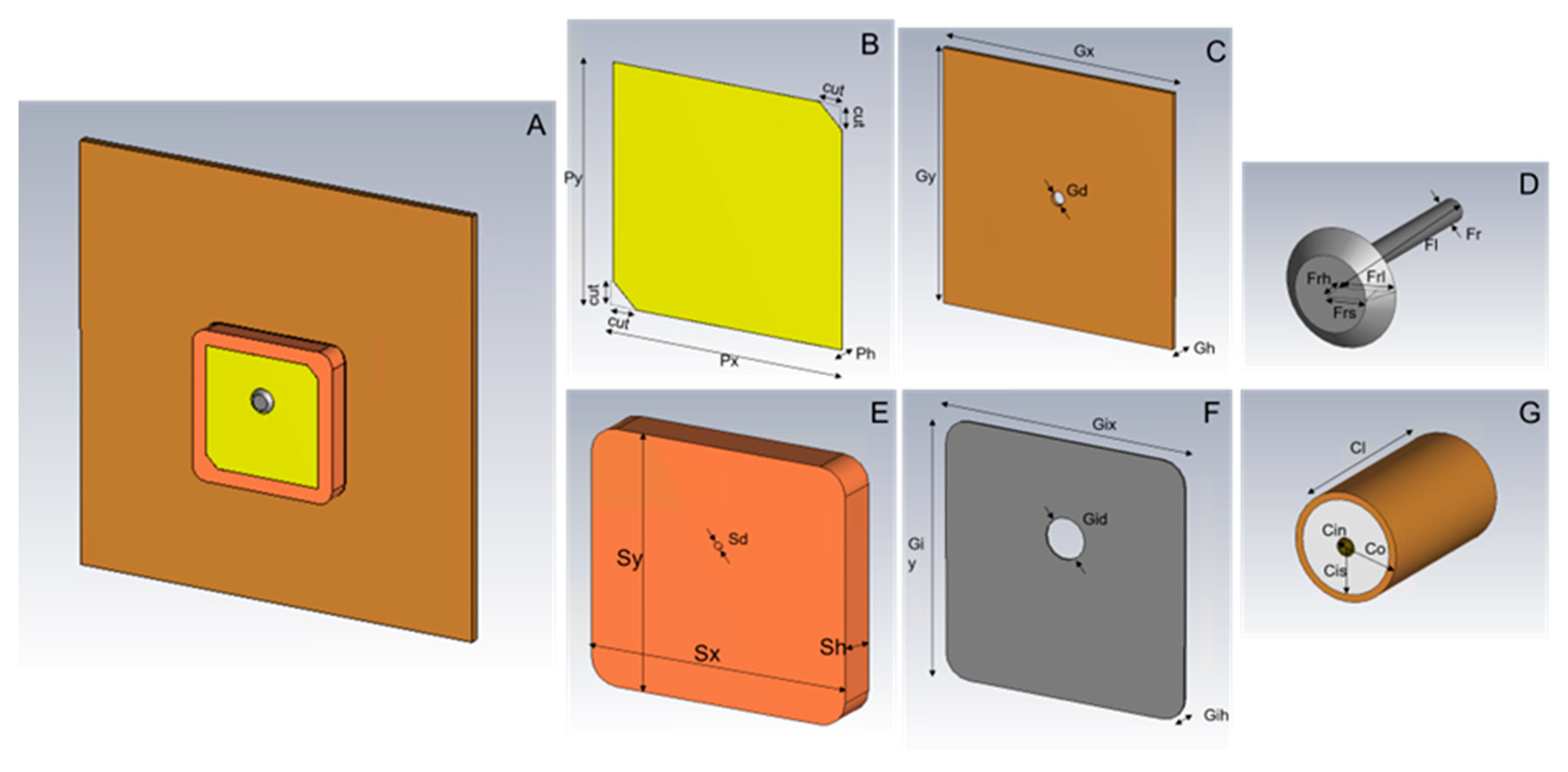
Figure 2.
A) Simulated vs B) datasheet-provided S11 and Axial Ratio in the φ=0˚, θ=90˚ direction.
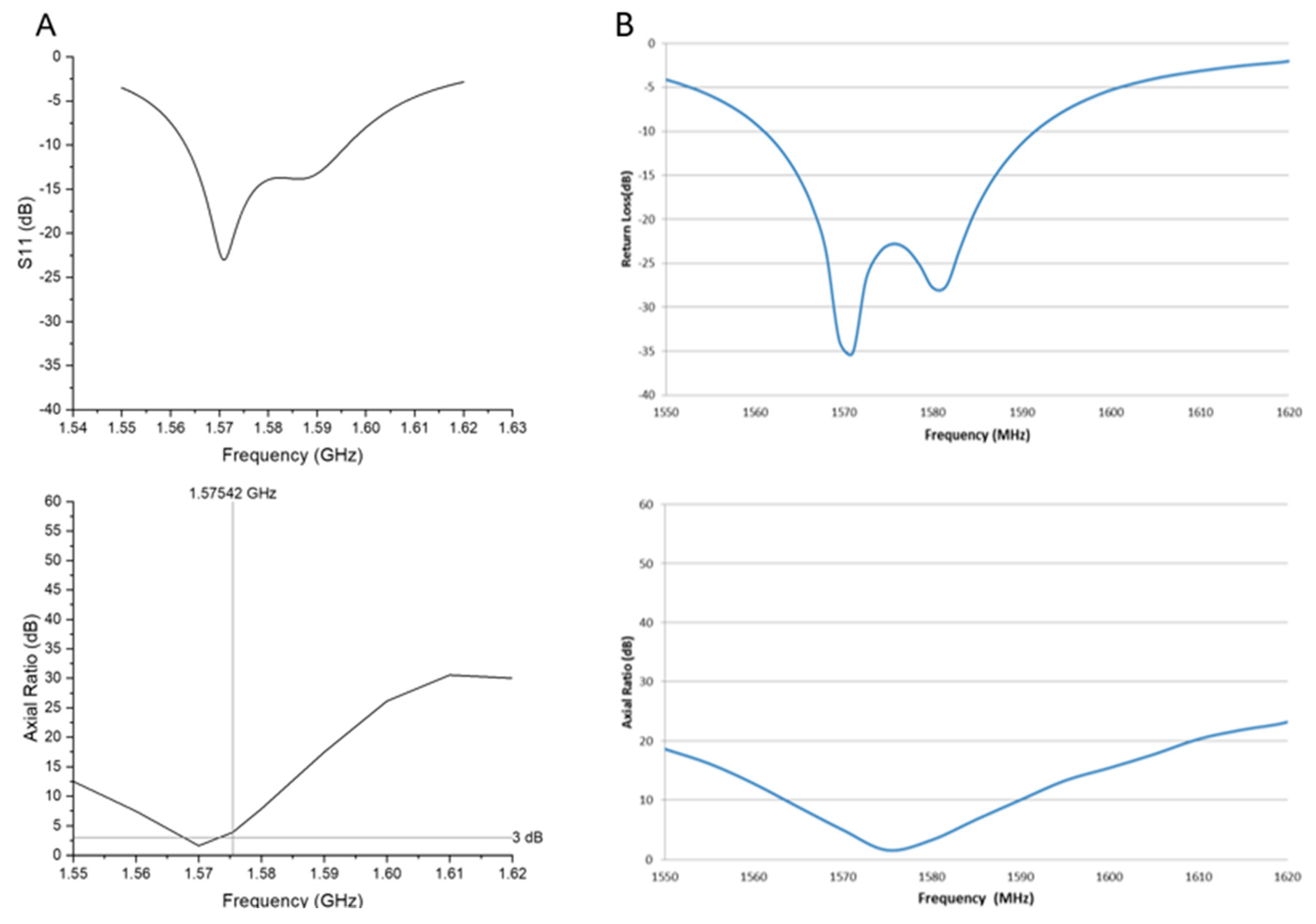
Figure 3.
Axial ratio at 1.57542 GHz in the elevation plane for φ=0˚˚ (A) and φ=90˚ (B).
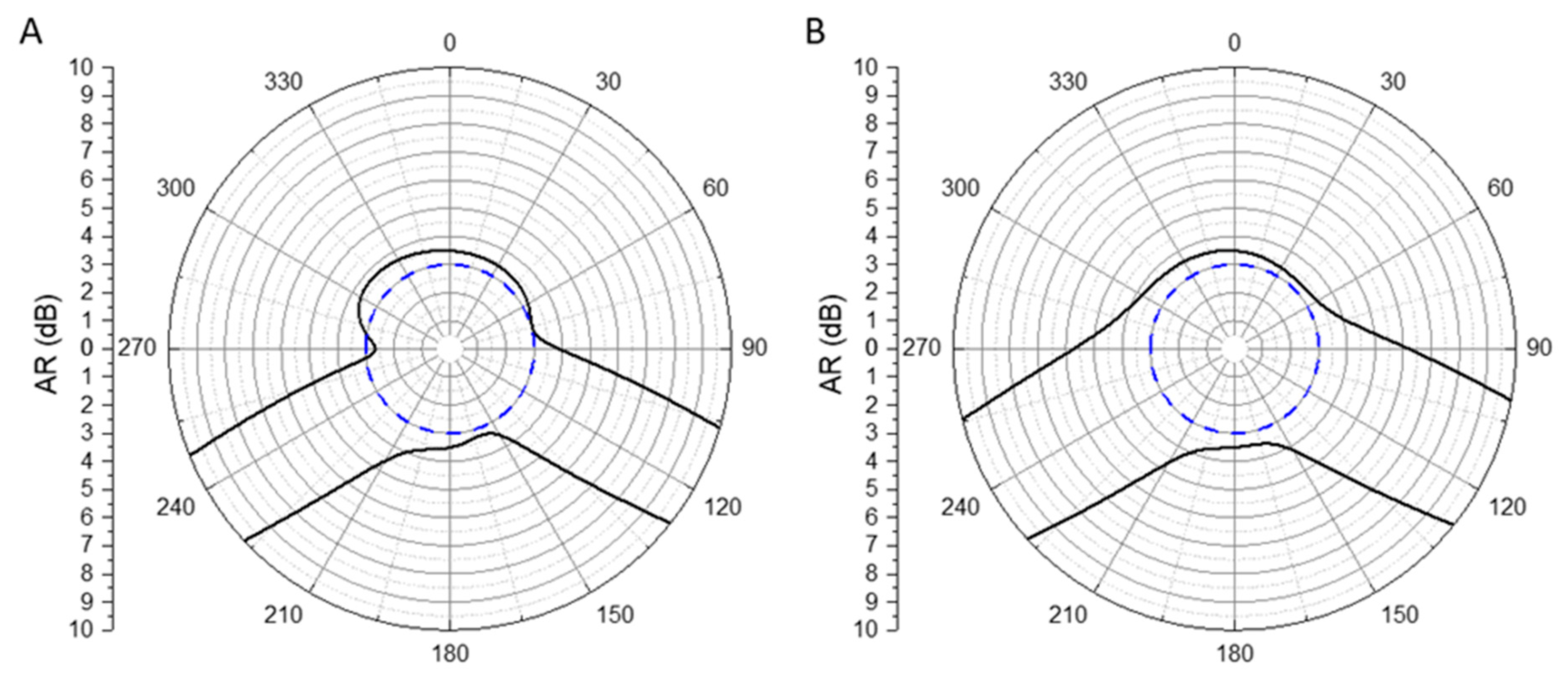
Figure 4.
Realized gain plot at 1.57542 GHz in the elevation plane for φ=0˚ (A) and φ=90˚ (B) for LHCP and RHCP signals.
Figure 4.
Realized gain plot at 1.57542 GHz in the elevation plane for φ=0˚ (A) and φ=90˚ (B) for LHCP and RHCP signals.
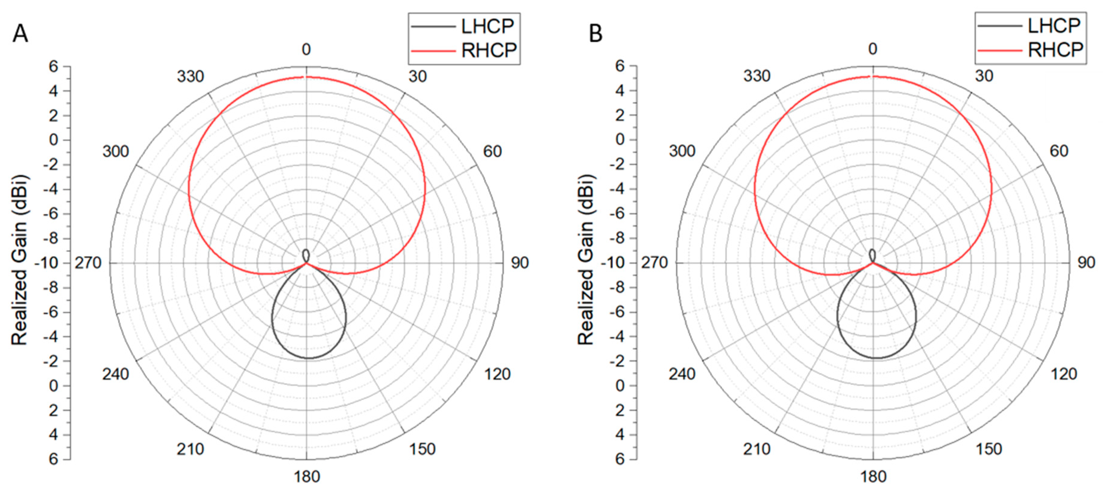
Figure 5.
Phase versus theta angle for φ = 0˚ (A) and φ = 90˚ (right) at 1.57542 for LHCP and RHCP signals.
Figure 5.
Phase versus theta angle for φ = 0˚ (A) and φ = 90˚ (right) at 1.57542 for LHCP and RHCP signals.

Figure 6.
CST model (A) and photograph (B) of the 4x4 array.
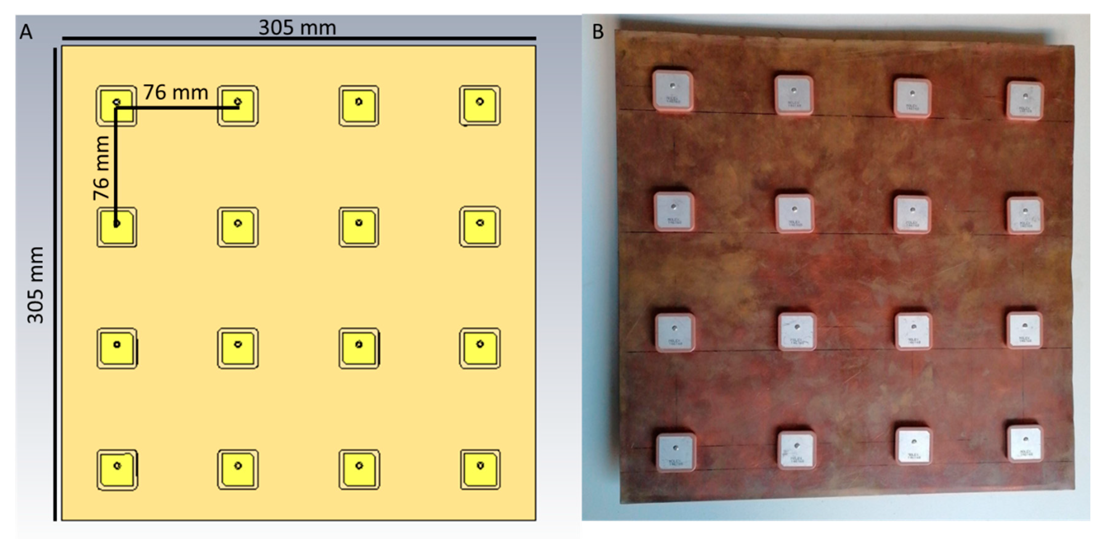
Figure 7.
D radiation pattern of the 4x4 array with the beam pointing to different (φ, θ) angles. A) (0, 0). B) (0, 45). C) (0, 90). D) (45, 45). E) (45, 90). F) (90, 45). G) (90, 90).
Figure 7.
D radiation pattern of the 4x4 array with the beam pointing to different (φ, θ) angles. A) (0, 0). B) (0, 45). C) (0, 90). D) (45, 45). E) (45, 90). F) (90, 45). G) (90, 90).
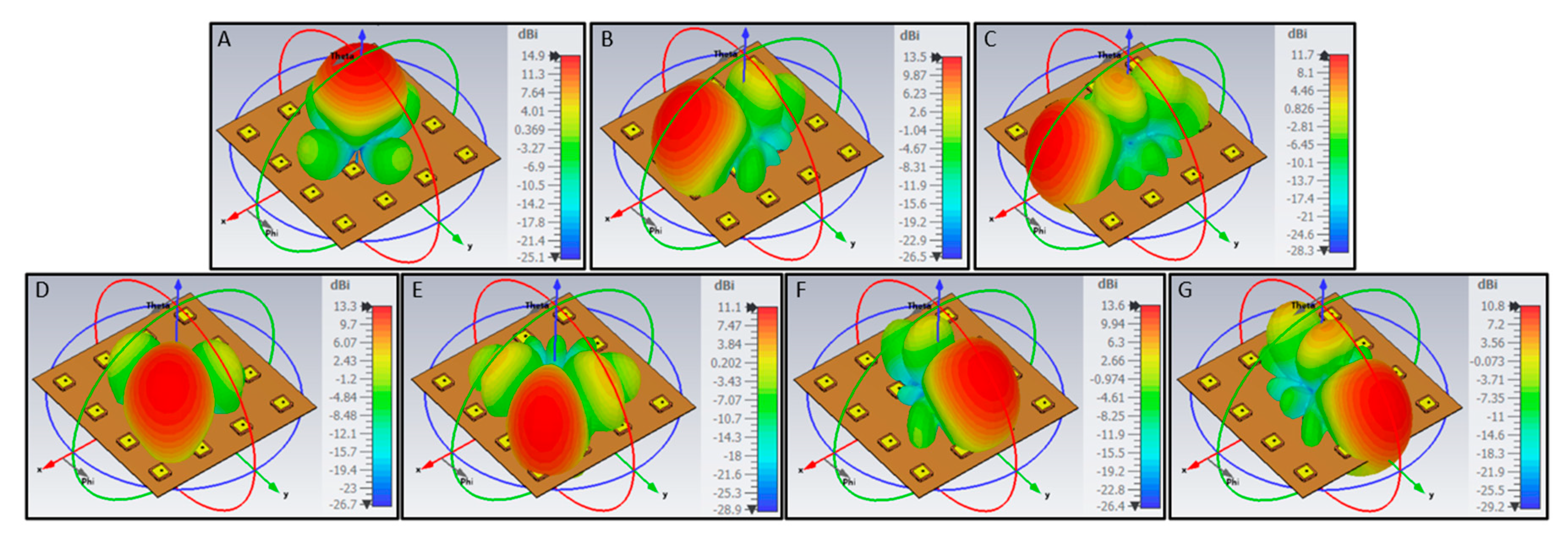
Figure 8.
Elevation plane radiation pattern of the 4x4 array with the beam pointing to different (φ, θ) angles. A) (0, 0). B) (0, 45). C) (0, 90). D) (45, 45). E) (45, 90). F) (90, 45). G) (90, 90). The red dashed lines represent the defined beamforming direction.
Figure 8.
Elevation plane radiation pattern of the 4x4 array with the beam pointing to different (φ, θ) angles. A) (0, 0). B) (0, 45). C) (0, 90). D) (45, 45). E) (45, 90). F) (90, 45). G) (90, 90). The red dashed lines represent the defined beamforming direction.
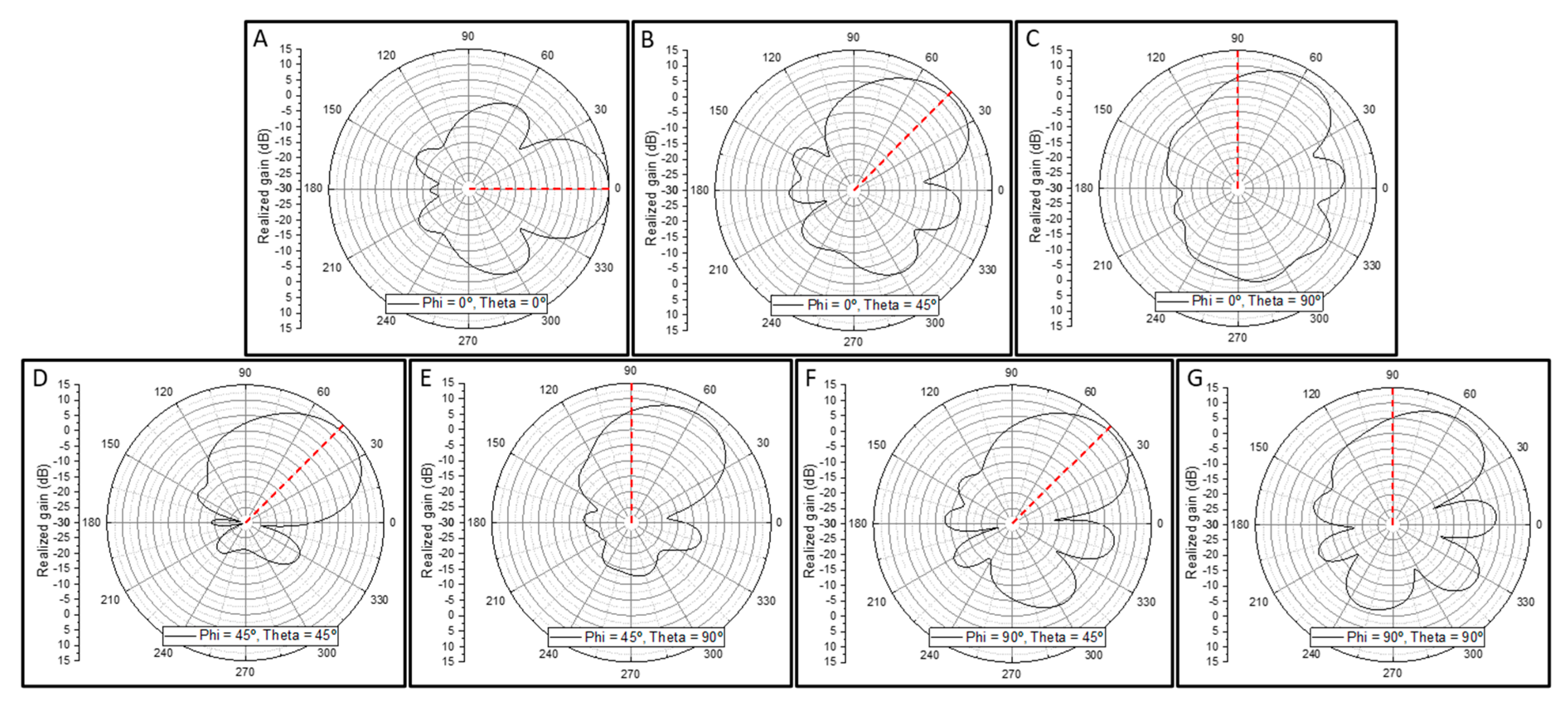
Figure 9.
- Axial ratio in the elevation plane of the 4x4 array with the beam pointing to different (φ, θ) angles. A) (0, 0). B) (0, 45). C) (0, 90). D) (45, 45). E) (45, 90). F) (90, 45). G) (90, 90). The red dashed lines represent the defined beamforming direction. The blue dashed circles correspond to a 3 dB AR.
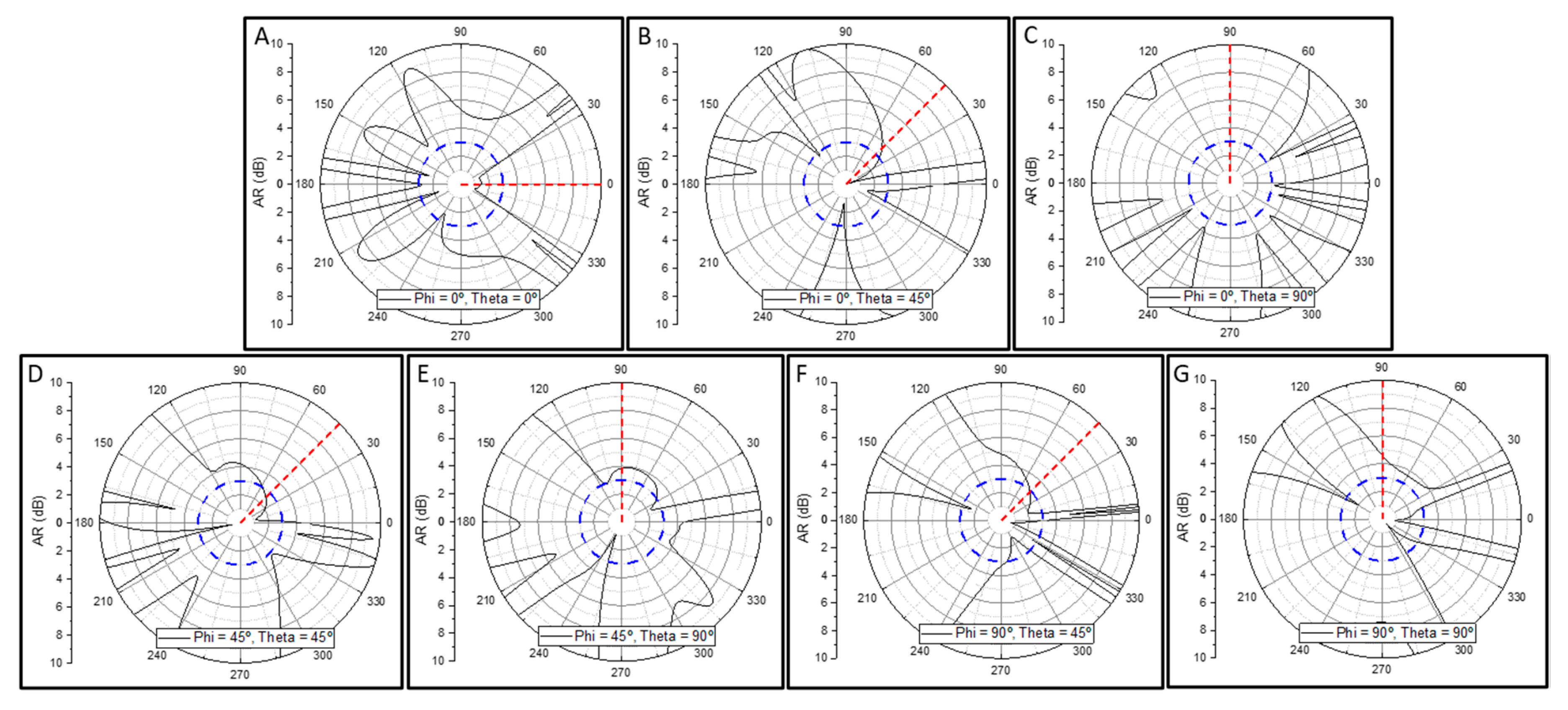
Figure 10.
- Block diagram of the employed ZCU216 digital beamforming system.
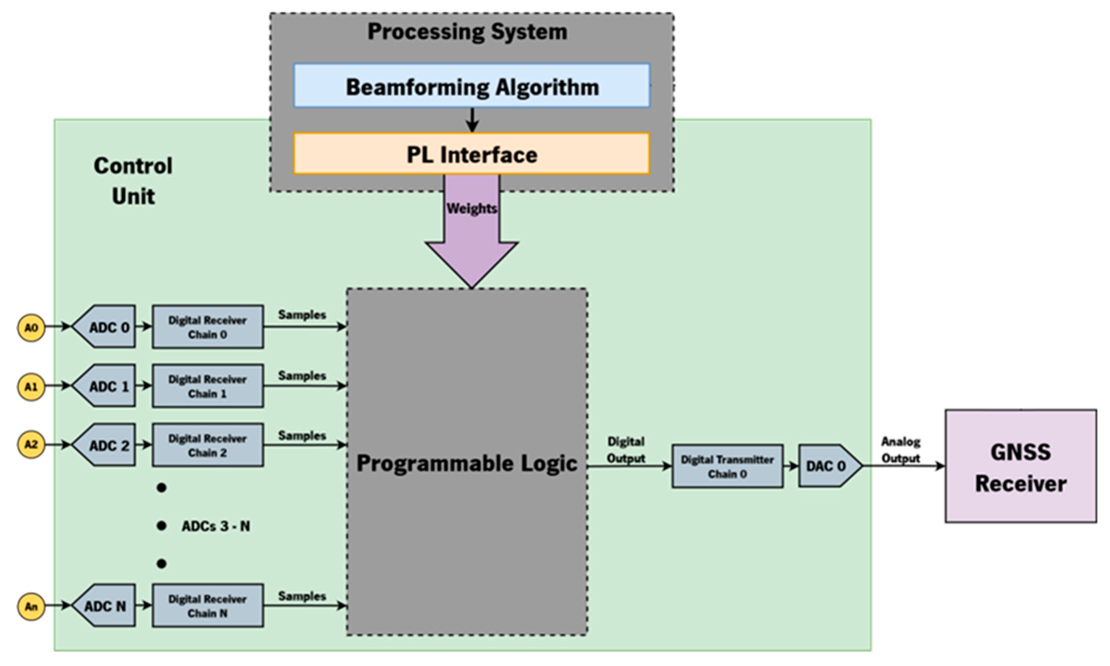
Figure 11.
– Planar array reference frame.
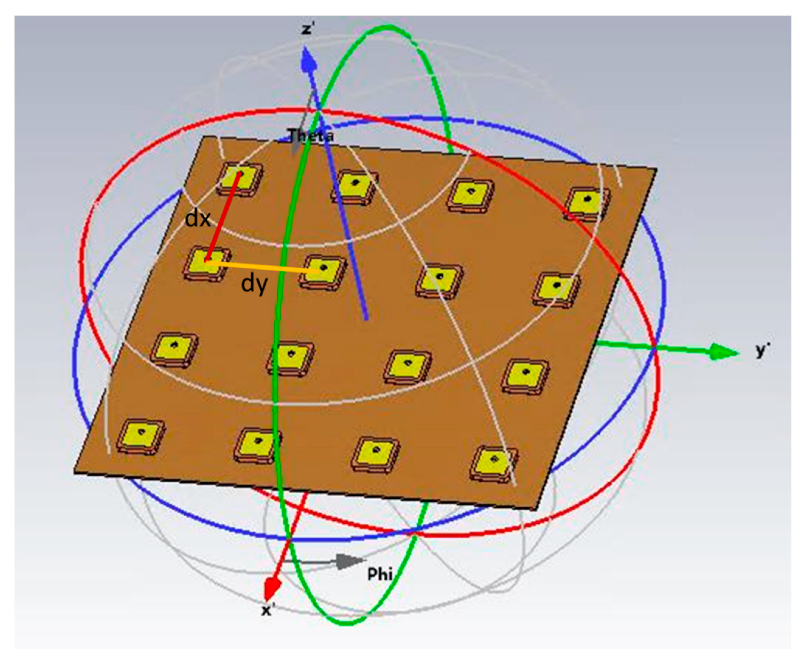
Figure 12.
- Antenna array and ZCU216-based ABDP inside the anechoic chamber for radiation pattern measurement.
Figure 12.
- Antenna array and ZCU216-based ABDP inside the anechoic chamber for radiation pattern measurement.
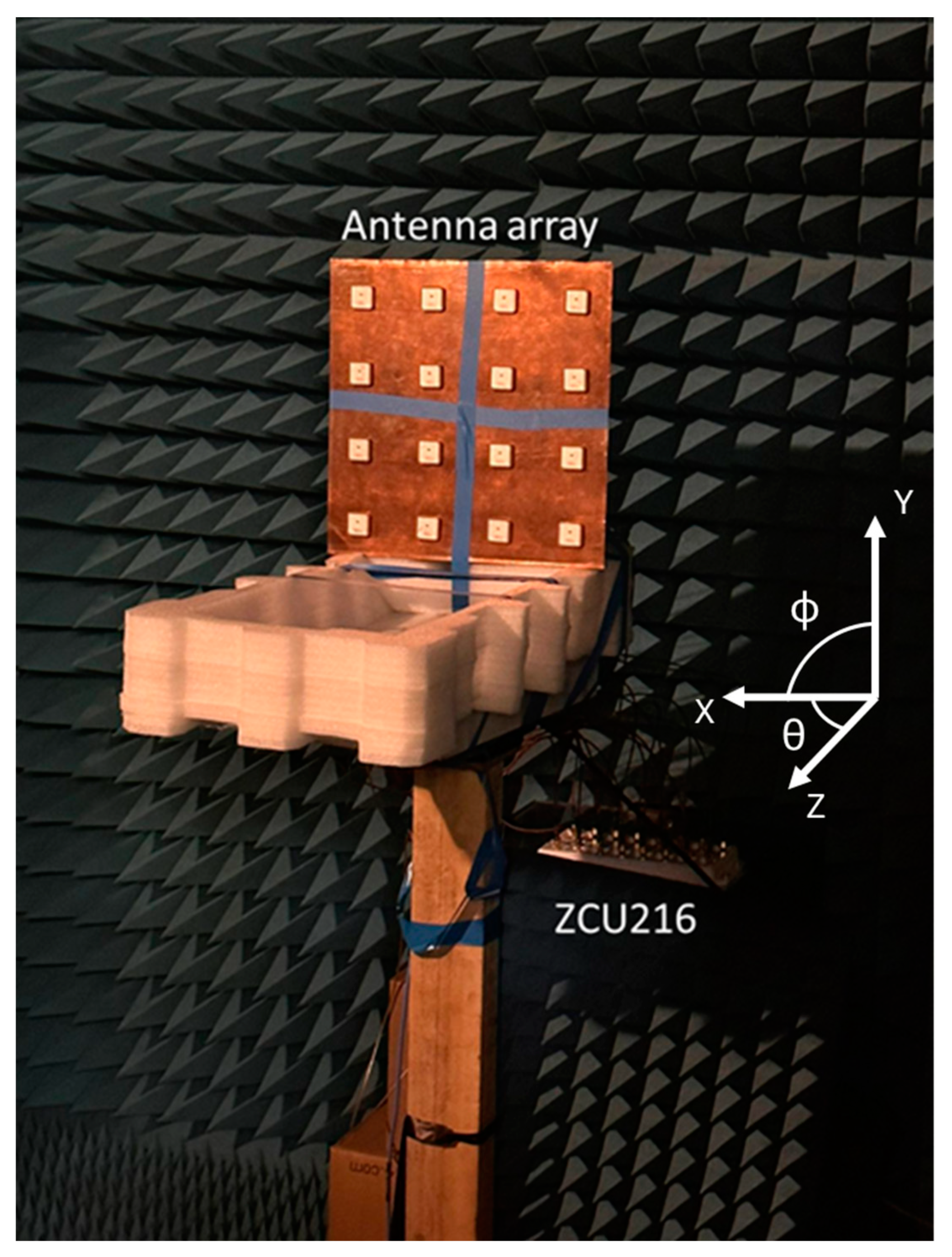
Figure 13.
– Measured and simulated single beam azimuth radiation patterns at φ = 0˚ with the main beam pointing towards: A) θ = 0˚, B) θ = 340˚, C) θ = 60˚ and D) θ = 300˚.
Figure 13.
– Measured and simulated single beam azimuth radiation patterns at φ = 0˚ with the main beam pointing towards: A) θ = 0˚, B) θ = 340˚, C) θ = 60˚ and D) θ = 300˚.
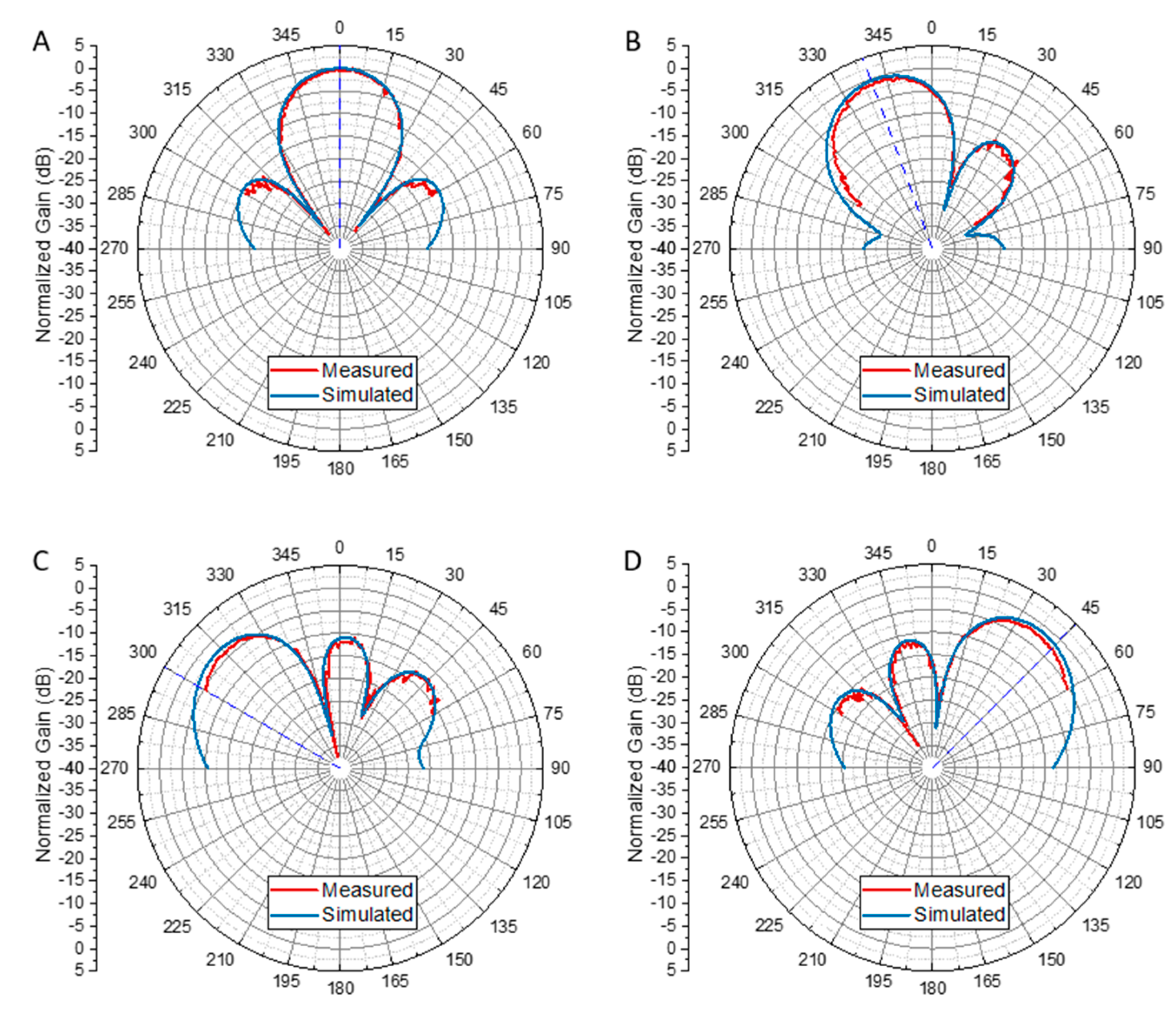
Figure 14.
- Measured and simulated single beam azimuth radiation patterns at φ = 45˚ with the main beam pointing towards: A) θ = 0˚, B) θ = 340˚, C) θ = 60˚ and D) θ = 300˚.
Figure 14.
- Measured and simulated single beam azimuth radiation patterns at φ = 45˚ with the main beam pointing towards: A) θ = 0˚, B) θ = 340˚, C) θ = 60˚ and D) θ = 300˚.
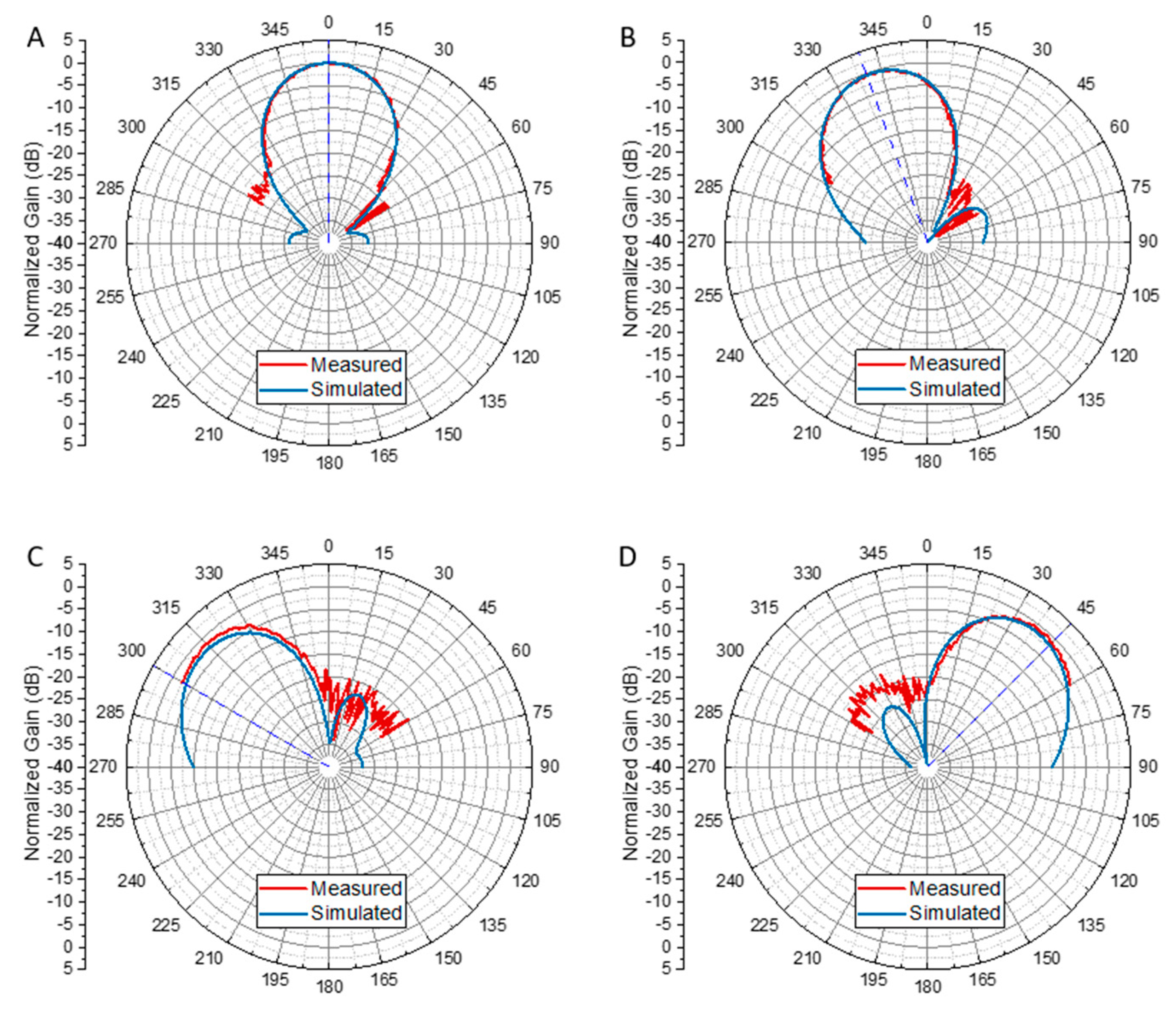
Figure 15.
- Measured and simulated multibeam azimuth radiation pattern with beams pointing towards θ = 0˚, θ = 45˚ and θ = 330˚. The dashed blue lines indicate the target main beam directions.
Figure 15.
- Measured and simulated multibeam azimuth radiation pattern with beams pointing towards θ = 0˚, θ = 45˚ and θ = 330˚. The dashed blue lines indicate the target main beam directions.
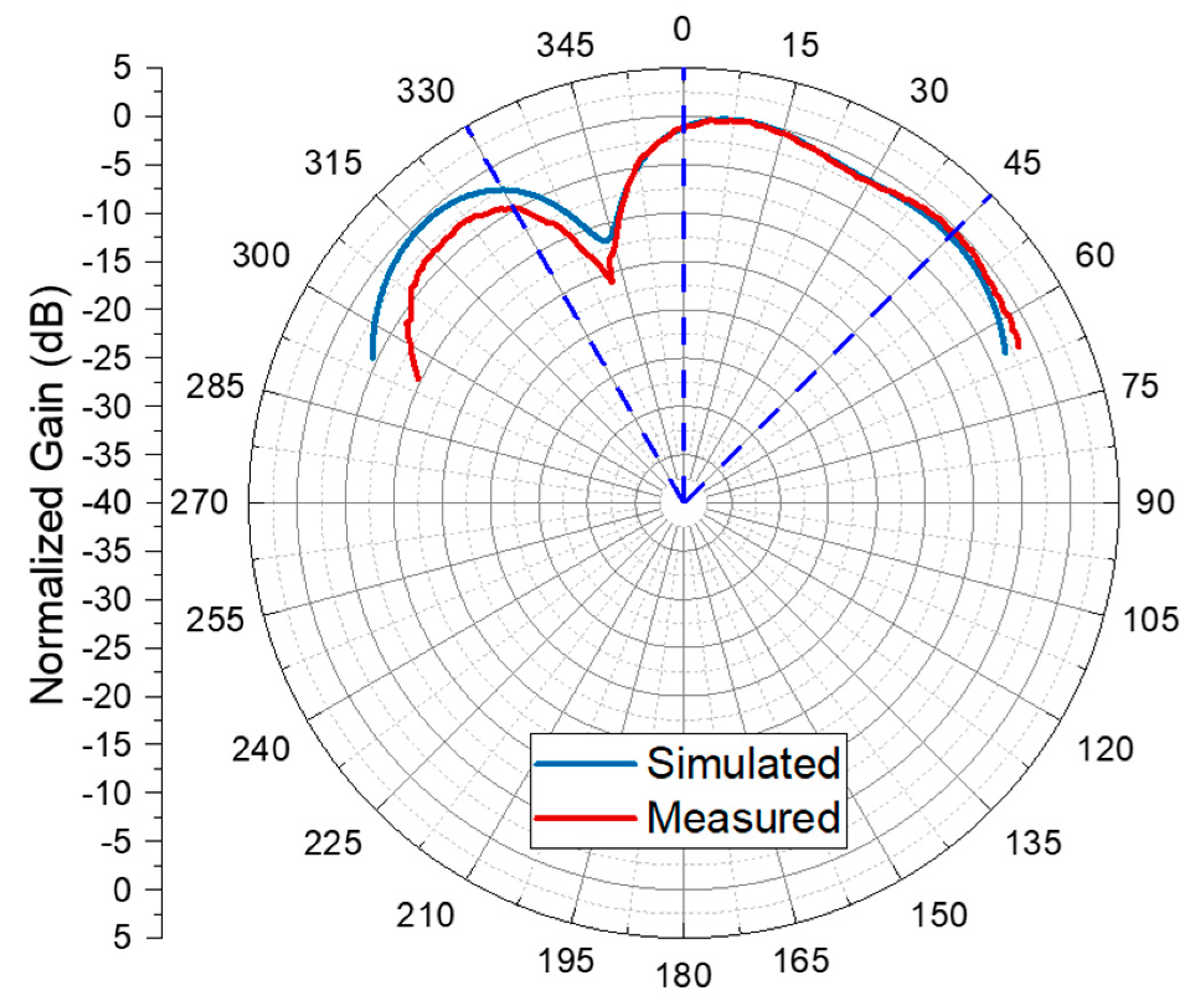

Table 1.
COTS antenna geometry parameters.
| Figure 1 | Parameter | Value (mm) | Material |
|---|---|---|---|
| B | Px | 20 | Silver |
| Py | 20 | ||
| Ph | 0.01 | ||
| cut | 2 | ||
| C | Gx | 70 | Copper (annealed) |
| Gy | 70 | ||
| Gh | 1.5 | ||
| D | Fr | 0.4 | Copper (annealed) |
| Fl | 7 | ||
| Frs | 2.6 | ||
| Frl | 3.98 | ||
| Frh | 0.69 | ||
| E | Sx | 25 | Ceramic εr=20.65 |
| Sy | 25 | ||
| Sh | 4 | ||
| Sd | 0.4 | ||
| F | Gix | 24.6 | Copper (annealed) |
| Giy | 24.6 | ||
| Gih | 0.2 | ||
| Gid | 4 | ||
| G | Cin | 0.64 | Gold |
| Cis | 2.13 | Vaccum | |
| Co | 2.64 | Copper (annealed) | |
| Cl | 15 | - |
Disclaimer/Publisher’s Note: The statements, opinions and data contained in all publications are solely those of the individual author(s) and contributor(s) and not of MDPI and/or the editor(s). MDPI and/or the editor(s) disclaim responsibility for any injury to people or property resulting from any ideas, methods, instructions or products referred to in the content. |
© 2025 by the authors. Licensee MDPI, Basel, Switzerland. This article is an open access article distributed under the terms and conditions of the Creative Commons Attribution (CC BY) license (http://creativecommons.org/licenses/by/4.0/).
Copyright: This open access article is published under a Creative Commons CC BY 4.0 license, which permit the free download, distribution, and reuse, provided that the author and preprint are cited in any reuse.


