
Submitted:
20 February 2025
Posted:
20 February 2025
You are already at the latest version
Abstract
Due to the rise of gigascale antenna arrays considered to implement long-range wireless power transfer (WPT), there is a need for a scalable high-efficiency adaptive dynamic beam focusing method. Several methods have been proposed ranging from methods requiring position information of the receiver, use of pilot signals or channel sounding, and feedback-based approaches. The latter has the potential to achieve maximum WPT efficiency due to use of feedback between the rectenna target and the transmitter array. In this paper, we present an overview of the different feedback-based long-ranged WPT methods that have been proposed. We also evaluate them in terms of convergence time, complexity of implementation, and steady-state efficiency through a simulation. The results show that methods that measure channel state information (CSI) and the both-sides retrodirective system can achieve high efficiency with less convergence time, but with added implementation complexity.
Keywords:
wireless power transfer
; dynamic beam focusing
; gigascale antenna arrays
; microwave power transfer
; channel state information estimation
; far-field
; retrodirective arrays
; time reversal
1. Introduction
Long-range wireless power transfer is expected to have an antenna array considered to be "Gigascale Antenna Arrays" [1]. Each antenna element on this transmitter array is expected to cooperate with each other to be able to accurately focus a power beam towards a rectenna array to achieve a high efficiency wireless power transfer (WPT). It must also achieve a task in a time-changing environment, thus, requiring the system to be controllable and adaptive. The act of changing the beam properties to a target area is called dynamic beam focusing [2].
The different methods that have been developed for this purpose can be broadly categorized into three types: 1) the conventional antenna array beam steering used in conjunction with position sensors [3,4,5], 2) use of pilot signals to guide the generator antennas [6,7], or 3) feedback control using data sent back by the receiver to the generator [2,5,8]. On all the approaches, there is generally a trade-off observed between the WPTE performance and the convergence time needed to achieve their steady state.
The first type requires position tracking of the receiver through image recognition, radar, or satellite positioning. Once the position is determined, the system uses traditional beam steering techniques [3,5]. The second type improves on the first by letting the receiver system send a pilot signal to the generator and then it performs wavefront reconstruction [5]. An optimal method to implement this is through the use of retrodirective antennas [7,9,10]. The time-reversal technique, which can be viewed as a wideband implementation of retrodirectivity, is also proposed [11,12]. In this, the channel’s impulse response as seen by the different transmitter elements is measured from the receiver’s beacon. Each transmitter element produces a mirror of the measured response producing a matched filter condition which focuses the power in the area of the corresponding receiver.
The third type of WPT beam focusing technique relies on a feedback mechanism which makes the system adaptive. Due to the use of feedback, this type of dynamic beam focusing technique has the potential of achieving maximum WPT efficiency predicted from the eigenvalue formulation regardless of channel configuration. Since this class of dynamic beam focusing techniques have the potential to perform well in a time-varying channel, it is of interest to review different works that have been developed classified under it. In this paper, we review and compare these methods in terms of their convergence time, steady-state efficiency, and complexity of implementation.
2. Mathematical Framework to Analyze the Steady-State Efficiency of WPT
2.1. Notation
Scalar quantities are written in italics, column vectors in lower case bold, and matrices in uppercase bold. For example, a and A are scalars, is a column vector, and is a matrix. The notation indicates a column vector for a positive integer set defined by i and is a matrix with a column index i and a row index j, both positive integers. Since these are complex quantities, we then define and as the magnitude and phase of a, respectively.
The transpose and Hermitian transpose operations of are defined by and , respectively, and these operations transform a column vector into a row vector and vice versa. The per-element conjugation operation is denoted as . The three operations outlined above can also be applied to matrices. The conjugation operation can also be done on scalars.
We denote the superscript as the discrete-time index. The value of some quantity a, , or at some time is denoted by , , and , respectively. We differentiate this with the exponentiation notation where a is a base and k is an exponent. We denote and as the set of all real numbers and complex numbers, respectively. Finally, we define as the unit Heaviside step function.
2.2. Preliminary System Setup
For a system of N power generating antennas and M receiver antennas shown in Figure 1, let be the voltage at the ports on the receiver array and as those on the generator array [13]. Conveniently, the total power at the receiver and the transmitter can be expressed by and , respectively, where is the matched impedance assumed to be the same for all ports. The relationship between the voltages can be defined by the S-parameters shown in Figure 1 where and . Subscript indicates a forward wave, or a wave going in, and means backward wave, or a wave going out of the system and into the respective ports.
In Figure 1, the diagonal submatrices, and , describe the wave reflected back to their respective set of ports. Ideally, all their elements are zero. On the other hand, the non-diagonal submatrices indicate the waves that is transmitted from one set of ports to another. For example, represents the power sent from to and this is where we want power to flow. The wireless channel is assumed to be reciprocal implying that .
2.3. Maximum Theoretical WPT Efficiency
If there is an input at the power generators, the formula for the WPTE can be expressed as the ratio of the power at the receiver from to the input power at the generator from and this is expressed in Figure 2. This is called the Rayleigh coefficient which is widely used in different works when maximizing the WPTE of antenna arrays [2,14]. The maxima of this is the maximum eigenvalue of . Let be the eigenvalues of the matrix expression. Since is Hermitian, then for all eigenvalues. Then the maximum theoretical efficiency is governed by the largest possible as expressed in Figure 3.
2.4. WPT Efficiency of Any Transmitter Input Configuration
An arbitrary input to the generator array can be expressed as a weighted sum of the set of the normalized eigenvectors of . This is shown in Figure 4 where and is an eigenvector for all . This assumes that is a full rank matrix.
Now, the efficiency of any arbitrary input can be expressed in terms of the weights, , and eigenvalues, , as shown in Figure 5. This also shows that each is the WPTE of the corresponding beam mode, , and the efficiency is a weighted average of the individual efficiencies of each beam mode.
A scalar multiple of the eigenvector associated with , denoted by , is the optimum setting for the input. In the case that multiple eigenvectors are associated with , then the optimum input can be a linear combination of the eigenvectors. The power can be controlled by the magnitude of the weights. To achieve high efficiency WPT, a system must be designed such that the maximum WPTE condition, , is maintained as the channel changes over time.
3. Overview of Feedback-Based Dynamic Beam Focusing Techniques
3.1. Iterative Optimization Techniques
Feedback can be in the form of telemetry data sent from the receiver to the transmitter in conjunction with optimization techniques maximizing the received power computed using 6 [2,5].
Common optimization techniques can be used like gradient descent, Nelder-Mead method, random walk, or genetic algorithm. One work proposed to use orthogonal phase masks with phase sweeping [2]. In this method, each phase mask divides the transmitter antennas into two groups labelled "+1" and "-1" and phase sweeping is performed with the former increasing in phase and the latter decreasing in phase. The phase setting with the maximum power will be stored and a weighted sum of all of the maximum phases of each phase mask is computed at the end. Since the set of phase masks are orthogonal to each other, the optimal phase setting of each mask is independent to another. The result is an optimal phase setting for each antenna element in the transmit array. A secondary volumetric refocusing can be done afterward for changing channel conditions provided that the position is known.
Another proposed method is to optimize the antenna setting of each element one by one called the directional radiation by iterative optimization (DRIS) [5]. In this algorithm, an initial transmit antenna is set as to a reference phase. The next antenna’s transmit power and phase is optimized through an optimization algorithm maximizing the power received at the receiver. Once optimization is complete, the antenna settings are kept and the algorithm moves on towards the next transmit antenna element. Any optimization algorithm can be used for this purpose.
Beam scanning is also considered as a possible method to first detect the position of the target receiver and optimization is a secondary step like the directional radiation through area scanning (DRAS) [5] and look-up table based method [15], but these methods require additional hardware and processing.
To reduce the need for complex processing, a simple random walk optimization can be performed [16]. In this, a random initial transmission vector is set and a set of K random perturbations are computed. New weight vectors are computed from perturbations and the power of each of these are measured. The maximum setting is chosen and the algorithm will repeat itself until convergence is achieved. Although simple, achieving high WPT efficiency in this method is a hit or miss in terms of the perturbation setting, number of needed perturbations, and convergence criterion. Moreover, this method takes a longer time to converge which will be an issue for dynamic conditions.
Over-all, iterative methods provide a simple feedback mechanism through just establishing a communication channel between the transmitter and receiver, but the receiver will need to report the received power for every trial setting done by the transmitter. One big disadvantage of these methods is the possibility of converging to a local maxima.
3.2. Techniques That Use Channel Estimation
In the mathematical model of the WPT system, studying equations 3 and 5, the optimal transmitter setting to achieve maximum power transfer is an eigenvector of the matrix expression , where can be interpreted as the channel state information (CSI) that has been thoroughly studied in wireless communication systems [17]. If it is known, then the optimal eigenvector can be determined through numerical means [18,19].
An outstanding problem in this approach is the measurement capabilities of the receiver. CSI can be estimated better if the receiver is able to measure both amplitude and phase of the incoming signal from the transmitters, but this requires more complex hardware on the receiver side. A proposed workaround uses the power measured by the receiver and transmitted as telemetry data in the same way as iterative methods [8,20]. In these works, for a WPT system with N transmitters, if is the pilot signal for , , a process of "complex vectorization" is performed on the covariance matrix, , of defined in Equation 7.
Let the complex vectorization [8] of the pilot signal covariance matrix be expressed as . While is complex, the complex vectorization operation makes purely real. For each pilot signal sent, the power is measured as . Let the collection of K power measurements is expressed as and the set of pilot signals be expressed as . Once all of these are gathered, a complex vectorized estimate of the CSI matrix, , can be estimated through different estimation methods.
Two proposed estimation methods are the least squares estimate (LSE) and the Kalman filter (KF) estimate. Using the LSE method, Equation 8 is used. Of the two methods, the latter takes into account historical measurement data, while the former considers only the new set of measurements.
Another proposed channel estimation method that directly uses the model proposed in Figure 1 in conjunction with Equation 1 [21]. Noting that the S parameters can be expressed as , then can be estimated as the square root of the power received from one transmitter to one receiver while can be estimated from the relative distances between the transmitter elements. This method, while simpler, has a worse performance compared to using the complex vectorization method because the estimation method being rooted in the far-field assumptions, which is not applicable to most WPT applications.
In general, more pilot signals can yield greater accuracy in estimation. However, this will increase the time required for the transmitter to compute the estimate. This is a huge disadvantage of channel estimation methods for WPT applications, but its merit can be found in simultaneous wireless information and power transfer (SWIPT) applications.
3.3. Both-Sides Retrodirective Beamforming System
In the second class of dynamic beam focusing techniques, a pilot signal is used in conjunction with retrodirective arrays or time-reversal arrays to detect the direction of the incoming beam at the transmitter. By enabling this on both the transmitter and receiver, a form of feedback loop is created in which the pilot signal and the power beam reply are both constantly refined producing an optimum beam. This is called the both-sides retrodirective system [22]. This setup adaptively regenerates the pilot signal to changing channel conditions.
In a previous study done by the author [23], it was revealed that for an initial transmitter configuration expressed in Equation 9, the zero-input response of this system can be determined as shown in Equation 10. Here, are the initial weights of the eigenvectors defined previously from Equation 4, G is the loop gain of the system, are the eigenvalues, and is the transmit signal after k iterations.
Imposing a marginal stability condition on this system leaves an optimum beam, but achieving this is still an active area of inquiry. Due to the simplicity of the retrodirective system, this method can be scalable compared to the channel estimation approach and the iterative optimization approach. However, maintaining marginal stability is required, else risking the saturation power amplifiers when the system becomes unstable, or the signal dying down when the system becomes stable.
3.4. Summary
Over-all, there is a trade-off between complexity, convergence time, and efficiency of the feedback-based beam-focusing methods. Each method has their own advantages and disadvantages with iterative methods being the least efficient and slowest to converge, but simplest in implementation. Techniques that require channel estimation are the most complex in terms of implementation, but offers faster convergence time and more efficiency as long as estimation error is low. Additionally, they are compatible with future SWIPT systems. Finally, the both-sides retrodirective system balances all these requirements and is also scalable.
4. Simulation and Comparison Methodology
The three different types of feedback-based methods are compared in terms of convergence time and steady-state efficiency. Three (3) different simulation environments detailed in a subsection below will be used as the testbeds for comparison. The S-parameters computed from each is used in MATLAB for further simulation of the different types of dynamic beam focusing method.
4.1. Comparison Metrics
4.1.1. Convergence Time
Since the different methods require feedback between transmitter and receiver, each iteration requires a one (1) roundtrip. Thus, the number of iterations for a technique before reaching their respective convergence condition is synonymous to the convergence time of the system. A key assumption for this metric is that all computations done by the transmitter (e.g. channel estimation, conjugation, optimization, etc.) happens in an instant.
4.1.2. Steady-State Efficiency
4.2. Simulation Environments
The simulation environments are all modelled in Ansys HFSS as shown in Figure 2. A 23.7 mm × 23.7 mm square patch antenna was used as an element for all transmitter arrays. The dielectric used is the Arlon TC600 with a relative permittivity of and thickness of 2.54 mm. For a array, the total dimensions are 125 mm × 125 mm while for the arrays, it is 250 mm × 250 mm. All simulations were computed at 2.4 GHz center frequency.
4.3. Simulation Setup
4.3.1. Iterative Optimization Techniques
The orthogonal phase mask approach [2], DRIS [5] using Nelder-Mead, and random walk approach [16] are used in the comparison. For the first, the recommended orthogonal phase mask generated from the Hadamard matrix is used. For DRIS, the Nelder-Mead method [24] with a convergence condition of , reflection coefficient , reflection coefficient , contraction coefficienct , and shrinkage coefficient is used. Lastly, the convergence condition for the random walk is set to .
4.3.2. Techniques That Use Channel Estimation
The LSE-based approach [8] is used for comparison. The recommended pilot signal is used for the simulation in that for N transmitter antennas, N pilot signals composed of one (1) transmitting elements and pilot signals composed of a combination of two (2) transmitting elements were used for their linear independence property. This amounts to a total of pilot signals which is the minimum amount needed to make an estimate for the CSI.
4.3.3. Both-Sides Retrodirective Beamforming System
For this setup, the transmitter and receiver signal both conjugates the vectors that respectively arrive to them. If is the power beam vectors at the time index k, then Equation 11 is used to determine their values for the next iteration.
The initial condition is set to for all i, i.e., all eigenvectors of the transmission channel are initially energized.
5. Results and Discussion
Figure 3 show the progression of efficiency measured at each iteration of the different methods compared. The both-sides retrodirective system and the CSI using LSE consistently achieve the maximum theoretical efficiency while the iterative-based methods do not. This is due to the presence of local maxima when performing optimization. Thus, using iterative methods for WPT applications will have a tendency to converge into these sub-optimal conditions, especially for a dynamic environment or a setup with the presence of many scatterers.
Table 1 lists the total number of iterations needed by each method to finish their processing or achieve their respective convergence conditions. The results show that each of these feedback-based methods can get close to the maximum efficiency allowed by the channel conditions. The iterative feedback methods require a long convergence time to achieve a high performance with the random walk method needing the most amount of iterations. This can be attributed to the nature and simplicity of its implementation. In contract, the CSI estimation using LSE and both-sides retrodirective system boasts the least convergence time needed to achieve the maximum possible WPT efficiency, but their implementation is more complex compared to the iterative methods.
6. Conclusions
In this paper, we discussed the different types of dynamic beam focusing techniques broadly classifying them into three. The feedback-based approaches are also presented in more detail with their potential to adapt to dynamic environments and maintain maximum WPT efficiency the system offers. Comparison between the different proposed implementations through simulation for selected works were also presented. The convergence time and steady-state efficiency of each method were measured. Among them, CSI estimation methods and the both-sides retrodirective method consistently achieves maximum WPTE with a faster convergence time, but these added benefits come at the cost of a complex implementation, especially on the former. The simpler to implement iterative methods were shown to have a tendency to converge to sub-optimal conditions located in a local maxima for the different cases. These results confirms the hypothesis of a trade-off between complexity, convergence time, and steady-state efficiency among the different proposed implementations.
To expand on this work, a simulation of a dynamic channel condition is recommended to understand the performance of the different methods. Evaluating their robustness against noise or interference is also a good direction for future works.
Author Contributions
C.D. Ambatali is the sole author of this article.
Funding
This research received no external funding.
Institutional Review Board Statement
Not applicable.
Informed Consent Statement
Not applicable.
Conflicts of Interest
The authors declare no conflicts of interest.
References
- Pelham, T.; Chen, X.; Collins, B.; Parini, C.; Brown, A. An Overview of Gigascale Antenna Arrays and Electromagnetics for Space Based Solar Power. In Proceedings of the 2024 18th European Conference on Antennas and Propagation (EuCAP), 2024, pp. 1–4. [CrossRef]
- Hajimiri, A.; Abiri, B.; Bohn, F.; Gal-Katziri, M.; Manohara, M.H. Dynamic Focusing of Large Arrays for Wireless Power Transfer and Beyond. IEEE Journal of Solid-State Circuits 2021, 56, 2077–2101. [Google Scholar] [CrossRef]
- Yang, B.; Mitani, T.; Shinohara, N. Auto-Tracking Wireless Power Transfer System With Focused-Beam Phased Array. IEEE Transactions on Microwave Theory and Techniques 2023, 71, 2299–2306. [Google Scholar] [CrossRef]
- Anselmi, N.; Tosi, L.; Rocca, P.; Toso, G.; Massa, A. A Self-Replicating Single-Shape Tiling Technique for the Design of Highly Modular Planar Phased Arrays—The Case of L-Shaped Rep-Tiles. IEEE Transactions on Antennas and Propagation 2023, 71, 3335–3348. [Google Scholar] [CrossRef]
- Hui, Q.; Jin, K.; Zhu, X. Directional Radiation Technique for Maximum Receiving Power in Microwave Power Transmission System. IEEE Transactions on Industrial Electronics 2020, 67, 6376–6386. [Google Scholar] [CrossRef]
- Matsumuro, T.; Ishikawa, Y.; Mitani, T.; Shinohara, N.; Yanagase, M.; Matsunaga, M. Study of a single-frequency retrodirective system with a beam pilot signal using dual-mode dielectric resonator antenna elements. Wireless Power Transfer 2017, 4, 132–145. [Google Scholar] [CrossRef]
- Koo, H.; Bae, J.; Choi, W.; Oh, H.; Lim, H.; Lee, J.; Song, C.; Lee, K.; Hwang, K.; Yang, Y. Retroreflective Transceiver Array Using a Novel Calibration Method Based on Optimum Phase Searching. IEEE Transactions on Industrial Electronics 2021, 68, 2510–2520. [Google Scholar] [CrossRef]
- Choi, K.W.; Kim, D.I.; Chung, M.Y. Received Power-Based Channel Estimation for Energy Beamforming in Multiple-Antenna RF Energy Transfer System. IEEE Transactions on Signal Processing 2017, 65, 1461–1476. [Google Scholar] [CrossRef]
- Miyamoto, R.; Itoh, T. Retrodirective arrays for wireless communications. IEEE Microwave Magazine 2002, 3, 71–79. [Google Scholar] [CrossRef]
- DiDomenico, L.; Rebeiz, G. Digital communications using self-phased arrays. IEEE Transactions on Microwave Theory and Techniques 2001, 49, 677–684. [Google Scholar] [CrossRef]
- Li, B.; Liu, S.; Zhang, H.L.; Hu, B.J.; Zhao, D.; Huang, Y. Wireless Power Transfer Based on Microwaves and Time Reversal for Indoor Environments. IEEE Access 2019, 7, 114897–114908. [Google Scholar] [CrossRef]
- Cangialosi, F.; Grover, T.; Healey, P.; Furman, T.; Simon, A.; Anlage, S.M. Time reversed electromagnetic wave propagation as a novel method of wireless power transfer. In Proceedings of the 2016 IEEE Wireless Power Transfer Conference (WPTC), 2016, pp. 1–4. [CrossRef]
- Yuan, Q. S-Parameters for Calculating the Maximum Efficiency of a MIMO-WPT System: Applicable to Near/Far Field Coupling, Capacitive/Magnetic Coupling. IEEE Microwave Magazine 2023, 24, 40–48. [Google Scholar] [CrossRef]
- Oliveri, G.; Poli, L.; Massa, A. Maximum Efficiency Beam Synthesis of Radiating Planar Arrays for Wireless Power Transmission. IEEE Transactions on Antennas and Propagation 2013, 61, 2490–2499. [Google Scholar] [CrossRef]
- Bae, J.; Yi, S.H.; Koo, H.; Oh, S.; Oh, H.; Choi, W.; Shin, J.; Song, C.M.; Hwang, K.C.; Lee, K.Y.; et al. LUT-Based Focal Beamforming System Using 2-D Adaptive Sequential Searching Algorithm for Microwave Power Transfer. IEEE Access 2020, 8, 196024–196033. [Google Scholar] [CrossRef]
- Yedavalli, P.S.; Riihonen, T.; Wang, X.; Rabaey, J.M. Far-Field RF Wireless Power Transfer with Blind Adaptive Beamforming for Internet of Things Devices. IEEE Access 2017, 5, 1743–1752. [Google Scholar] [CrossRef]
- Han, Y.; Jin, S.; Wen, C.K.; Ma, X. Channel Estimation for Extremely Large-Scale Massive MIMO Systems. IEEE Wireless Communications Letters 2020, 9, 633–637. [Google Scholar] [CrossRef]
- Kato, H.; Yuan, Q. Array Factor, Retrodirective, and E-MIMO Beamforming Technologies. In Proceedings of the 2023 IEEE International Symposium On Antennas And Propagation (ISAP), 2023, pp. 1–2. [CrossRef]
- Ku, M.L.; Han, Y.; Lai, H.Q.; Chen, Y.; Liu, K.J.R. Power Waveforming: Wireless Power Transfer Beyond Time Reversal. IEEE Transactions on Signal Processing 2016, 64, 5819–5834. [Google Scholar] [CrossRef]
- Abeywickrama, S.; Samarasinghe, T.; Ho, C.K.; Yuen, C. Wireless Energy Beamforming Using Received Signal Strength Indicator Feedback. IEEE Transactions on Signal Processing 2018, 66, 224–235. [Google Scholar] [CrossRef]
- Wu, J.; Yuan, Q.; Okada, T.; Yang, B. An estimation method of the 4-port S-parameters used for the E-MIMO approach. Space Solar Power and Wireless Transmission 2024, 1, 148–151. [Google Scholar] [CrossRef]
- Matsumuro, T.; Ishikawa, Y.; Shinohara, N. Basic study of both-sides retrodirective system for minimizing the leak energy in microwave power transmission. IEICE Transactions on Electronics 2019, 102, 659–665. [Google Scholar] [CrossRef]
- Ambatali, C.D.; Nakasuka, S.; Yang, B.; Shinohara, N. Analysis and experimental validation of the WPT efficiency of the both-sides retrodirective system. Space Solar Power and Wireless Transmission 2024, 1, 48–60. [Google Scholar] [CrossRef]
- Nelder, J.A.; Mead, R. A Simplex Method for Function Minimization. The Computer Journal 1965, 7, 308–313. [Google Scholar] [CrossRef]
Figure 1.
The WPT system represented as a network of antennas which can be characterized by network parameters such as Z-, Y-, or S-parameters.
Figure 1.
The WPT system represented as a network of antennas which can be characterized by network parameters such as Z-, Y-, or S-parameters.
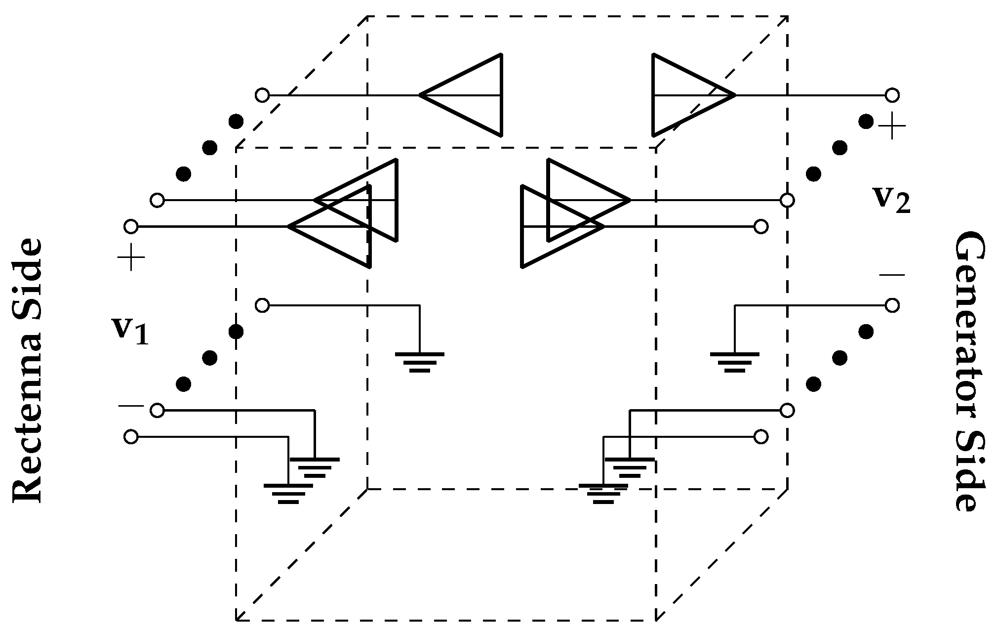
Figure 2.
The different simulation environments used for comparison: (a) A transmitter array sending power to two (2) receiver arrays obstructed by a perfectly conducting plate, (b) A transmitter array sending power to a receiver array, and (c) Three (3) distributed transmitter arrays cooperatively sending power to four (4) different dipole antennas.
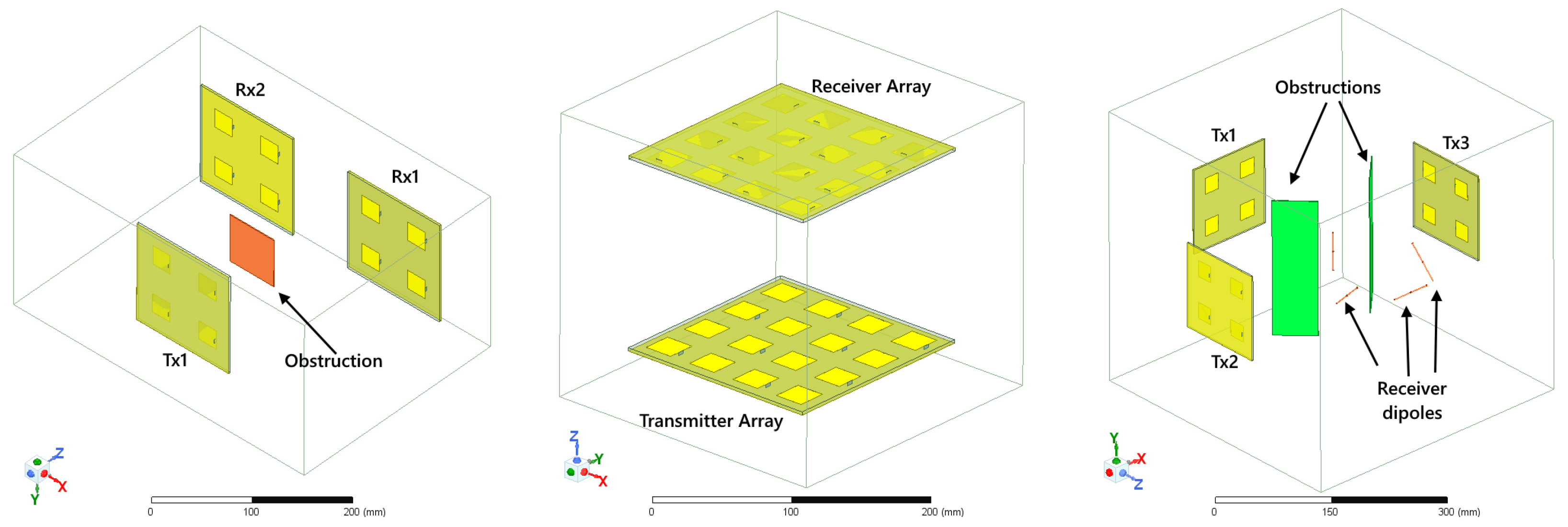
Figure 3.
Simulation results for: (a) A transmitter array sending power to two (2) receiver arrays obstructed by a perfectly conducting plate, (b) A transmitter array sending power to a receiver array, and (c) Three (3) distributed transmitter arrays cooperatively sending power to four (4) different dipole antennas.
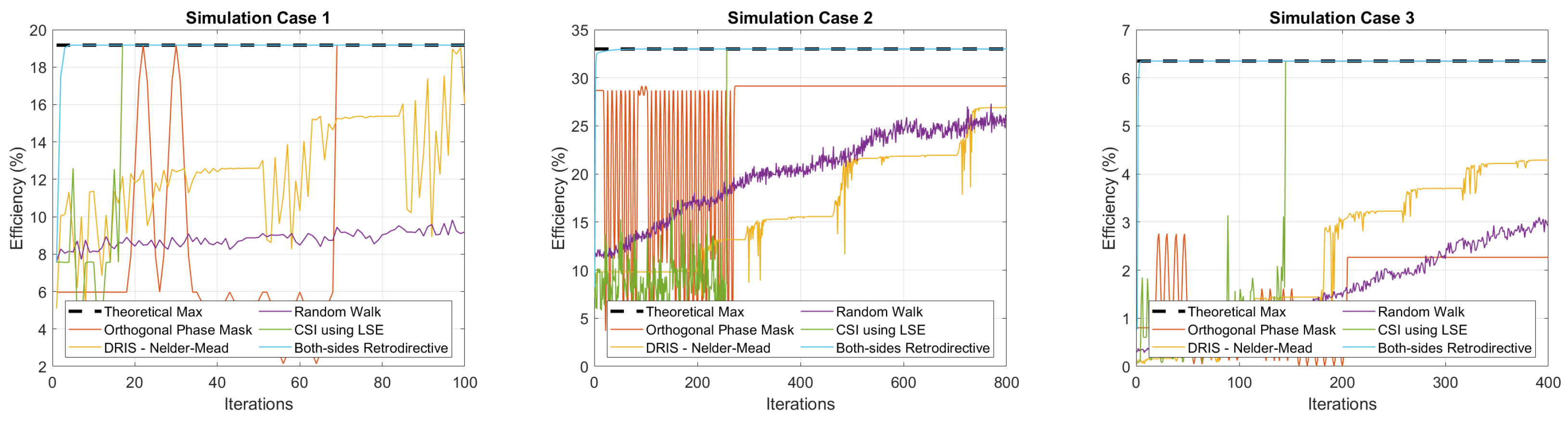

Table 1.
Number of iterations to converge and steady-state efficiency of each method.
| Method | Case 1 | Case 2 | Case 3 |
| Orthogonal Phase Mask [2] | 68 iterations | 272 iterations | 204 iterations |
| DRIS - Nelder-Mead [5] | 116 iterations | 1214 iterations | 606 iterations |
| Random Walk [16] | 3330 iterations | 6710 iterations | 1260 iterations |
| CSI estimation using LSE [8] | 17 iterations | 257 iterations | 145 iterations |
| Both-Sides Retrodirective | 5 iterations | 87 iterations | 5 iterations |
| System [22] |
Disclaimer/Publisher’s Note: The statements, opinions and data contained in all publications are solely those of the individual author(s) and contributor(s) and not of MDPI and/or the editor(s). MDPI and/or the editor(s) disclaim responsibility for any injury to people or property resulting from any ideas, methods, instructions or products referred to in the content. |
© 2025 by the authors. Licensee MDPI, Basel, Switzerland. This article is an open access article distributed under the terms and conditions of the Creative Commons Attribution (CC BY) license (http://creativecommons.org/licenses/by/4.0/).
Copyright: This open access article is published under a Creative Commons CC BY 4.0 license, which permit the free download, distribution, and reuse, provided that the author and preprint are cited in any reuse.


