
Submitted:
11 April 2025
Posted:
15 April 2025
You are already at the latest version
Abstract
Artificial lift (AL) methods are crucial for optimizing well performance and sustaining hydrocarbon production in oil and gas operations. Traditional AL selection relies on conventional methodologies and human expertise, which may be inadequate for handling complex reservoir dynamics and varying operating conditions. As the industry seeks more efficient, data-driven solutions, machine learning (ML) presents an opportunity to enhance AL selection. This study develops an ML-based stack framework of Random Forest (RF), Extreme Gradient Boosting (XGB) and Decision Tree (DT) to predict optimal AL methods. The models are trained and validated on a comprehensive dataset incorporating well particulars, production parameters, reservoir properties, and operational conditions. Performance evaluation demonstrates that the ML models achieve up to 95% accuracy in AL selection, significantly improving on traditional methods. The findings highlight the potential of ML-driven AL selection to enhance production efficiency, reduce operational costs, and optimize field performance. This study provides a foundation for integrating AI-based decision-making into artificial lift optimization, offering a more adaptive and precise approach to production engineering.
Keywords:
Artificial Lift
; Machine Learning
; Stack Model
; Production
; SHAP
1. Introduction
A key factor in maximizing well performance is the use of artificial lift (AL) techniques. These techniques are necessary to ensure a continuous extraction of hydrocarbons by overcoming the natural reduction in reservoir energy. Since AL is responsible for 95% of global oil production, it represents a significant milestone in the oil and gas sector. Sucker rod pumping (SRP), also known as beam pumping units (BPU), progressive cavity pumps (PCP), gas lift (GL), electrical submersible pumps (ESP), plunger lift (PL), hydraulic jet pumps (HJP), and hydraulic piston pumps (HPP) are among the various types of AL. About 70% of oil produced globally is produced using SRP, which is said to be the oldest lifting technique [1]. These artificial lifting techniques differ in their lifting capacities and conditions of use. For instance, sucker rod pumps used in low production wells have poor efficiency, electric submersible pumps are unsuitable for small displacement lifting, and surface-driven progressive cavity pumps in deviation wells have significant eccentric wear that shortens the pump inspection cycle [5]. Due to its successful operational history, gas lift (GL) is regarded as one of the most significant AL techniques globally [12].
In a situation where commodity prices are low, finding a means to reduce costs while increasing production is essential to the sustainability of ageing oil and gas fields. Frequently, a single well requires multiple artificial lift technologies to better recover gas and continually produce the hydrocarbon liquids [2]. Artificial lift selection techniques currently in use frequently depend on traditional approaches directed by human experience using qualitative methods. The fact that the field characteristics vary and rely on production years is a crucial concern. Furthermore, there is no theoretical or numerical correlation between the parameters, which results in inconsistent parameter selection and a laborious analytical process. As a result, additional costs arise from replacing AL in a short amount of time for manufacturing [1]. Machine learning (ML) serves as a valuable tool for enhancing human understanding of com-plex challenges and, in this context, offers a data-driven approach to artificial lift selection [4]. Within the oil and gas industry, ML has been widely applied in various do-mains, including data analysis [13], predictive modelling [14], and performance evaluation [15]. Choubey and Karmakar (2021) [16] examined the role that AI and ML approaches play in the oil and gas industry. Through an efficient selection of ML and AI methodologies, they offered a technical strategy that makes it possible to collect in-formation from large data in the sector. In addition to clustering, regression, and optimization, De Carvalho and Freitas (2009) [22] included classification issues as ML tasks. In ML and data mining domains, flat classification issues are split into two-class (binary) or multi-class problems. Both issues solely predict the classes at the structured leaf nodes and are single-label classification problems [21].
This study aims to innovate artificial lift selection techniques in oil and gas production by employing a robust machine learning framework. This framework, com-prising diverse machine learning models, aims to redefine selection practices with a dynamic and adaptive solution, enhancing accuracy significantly
2. Materials and Methods
2.1. Data Collection
The dataset utilized in this study comprises production data obtained from over 800 oil wells located within the Niger Delta Field. The wells selected for analysis are characterized by the implementation of artificial lift mechanisms to optimize hydrocarbon production. The dataset spans a time period from 2007 to 2021, providing a comprehensive representation of production dynamics over 14 years. The artificial lift methods employed include Gas Lift (GL), Sucker Rod Pump (SRP), Electrical Submersible Pump (ESP), Progressive Cavity Pump (PCP), Metal-to-Metal Progressive Cavity Pump (MTM PCP), and Hydraulic Lift (H_Lift). While Gas Lift and SRP are widely used in the region, MTM PCP and H_Lift have been applied in select cases, particularly in wells with high-viscosity crude or sand production challenges, which were a major concern in these particular wells. Some operators have explored these technologies through pilot programs and targeted deployments in complex reservoir conditions. The dataset was sourced from operational reports and field studies where these lift types were tested or implemented. The data contains features comprising oil production, gas production, water cut, GOR, sand production, amongst others. The distribution of these features is shown in Figure 1 below.
2.2. Well Selection Criteria
The selection of wells for inclusion in the dataset was based on specific criteria to ensure the representation of various reservoir and operational conditions. Wells were chosen based on their artificial lift status, with preference given to those employing techniques such as Gas Lift, Electric Submersible Pump (ESP), Progressive Cavity Pump (PCP), and others commonly utilized in the Niger Delta. Additionally, considerations were made regarding well productivity, reservoir characteristics, and historical performance data to ensure the diversity and relevance of the dataset.
2.3. Data Pre-Processing
Data pre-processing is a crucial and effort-intensive phase required to extract meaningful insights from raw data [20]. It involves applying various transformations to refine the dataset before feeding it into the machine learning algorithm. These transformations address issues such as missing values, outliers, and biased data [19]. To ensure consistency, accuracy, and relevance, the raw production data underwent extensive pre-processing. This included data cleaning techniques to detect and correct inconsistencies, remove outliers, and handle missing values. Since missing values accounted for less than 5% of the dataset and were randomly distributed, they were removed rather than imputed
Normalization was deemed unnecessary, as tree-based models are inherently robust to differences in feature scales. However, the dataset exhibited class imbalance, as shown in Figure 2, which could introduce an accuracy paradox if not addressed [7]. In this study, the data was deliberately left imbalanced to accurately represent field conditions and assess the model’s ability to generalize artificial lift selection [1]. Feature selection was also performed to minimize computational costs and prevent overfitting, as excessive features can negatively impact model performance [18]. Based on the available dataset, eight key features were identified for modelling: wellhead pressure, total fluid production, daily oil, gas, and water production, water cut, gas-oil ratio, and daily sand production. The Pearson correlation heatmap (Figure 2) illustrates the relationships between these variables, where positive values indicate that an increase in one variable leads to an increase in another, while negative values signify an inverse relationship.
2.4. Artificial Lift Classification
Figure 3 showcases the distribution of artificial lift (AL) methods across the dataset. It is evident that Sucker Rod Pump (SRP) emerges as the predominant lifting method within the field. However, despite GL’s prevalence, Figure 4 reveals that MTM_PCP and H_lift surpasses PCP and GL in cumulative oil production.
2.5. Machine Learning Modelling
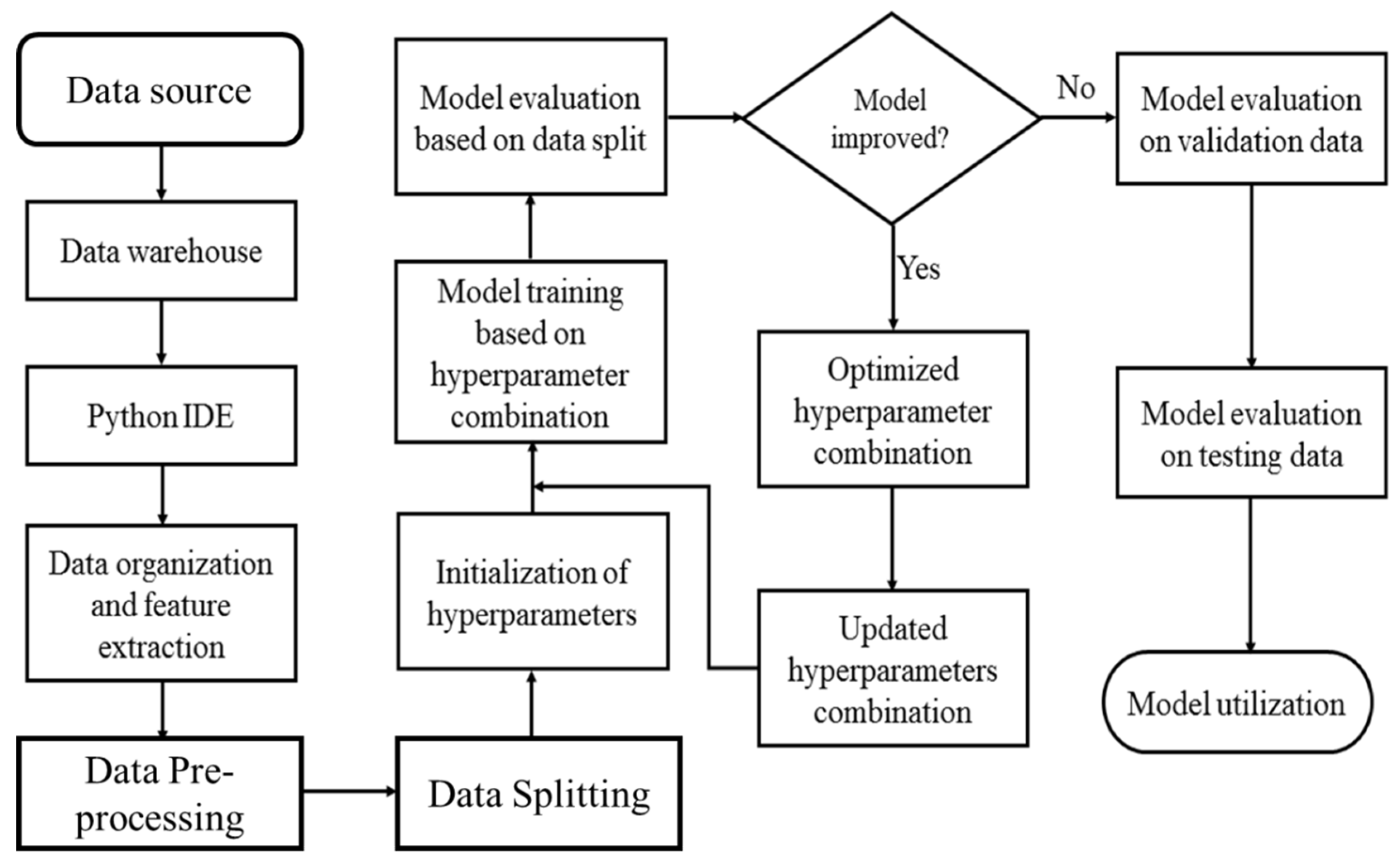
A flowchart illustrating the workflow used in the creation of the ML models used in this work is presented in Figure 4. A Microsoft Office Excel Workbook was used as a data warehouse to hold the data. Python was used for all data engineering and machine learning implementations, with Jupyter serving as the integrated development environment (IDE). Pandas and NumPy were used for all numerical computations. The specific machine learning models that were taken into consideration were the Meta Model, Logistic Regression (LR), and the base models, Random Forest (RF), Extreme Gradient Boosting (GB) and Decision Tree (DT). The dataset was divided into three subsets: training, validation, and testing, with a distribution ratio of 50:25:25, respectively. This partitioning strategy was adopted to prevent overfitting of the machine learning models to the training data. By allocating separate portions for validation and testing, totalling 50% of the dataset, we ensured robust evaluation metrics that were independent of the training process. Both the validation and test sets were reserved exclusively for evaluation purposes, thus providing a reliable assessment of model generalization and performance.
Figure 5.
Adopted Machine Learning Workflow.
The A.L. selection model is built using data and algorithms from over ten years of mature fields, which can be expressed as
or
Y = f (X)
Lift selection model = Algorithm (Field data)
Equation 1 [4] explains that the data quality determines the optimum AL selection. In supervised learning, the data are delivered to the algorithms, which are a collection of mathematical equations where the inputs X and outputs Y are given. By relating the input variables to the outputs and investigating the significance of each variable in the dataset, the algorithms are trained and learn. Based on training data, the algorithms then make the most accurate predictions for the fresh output (AL).
2.5.1. Machine Learning Models Utilised
- a.
- Random Forest
Random forest is a machine learning technique for developing prediction models in many research endeavours. It is based on a bootstrapping and aggregation approach called bagging [17]. Often in prediction modelling, a goal is to reduce the number of variables needed to obtain a prediction in order to reduce the burden of data collection and improve efficiency [6]. Every decision tree in the RF modelling process is given a random set of replacement input data (a bootstrap sample), and it develops on its own from there. The primary reason for the RF model's accuracy is the synergy that results from combining the predictions made by each decision tree. There are three steps in the RF process. Using the input variables, n bootstrapping samples are generated as the initial step. Utilising the maximal predictor split, an unpruned regression tree is constructed in the second phase, and the predictions from the n number of trees are aggregated in the final step [3]
For a random data subset , the decision tree iteratively partitions the variable space as samples with close targets are aggregated. The data at node m is represented by with samples. dm may be partitioned into subsets denoted as and using each candidate split where p and refer to a feature and threshold, respectively (Equation (2)).
The candidate split is defined as a loss function , as shown in Equation (3).
Where
The minimization of Equation (3) yields the parameters .
The recursion of Equation (4) continues for and until the maximum depth is achieved. The prediction of the RF model is thus obtained from Equation (5).
where K is the number of decision trees (DT) in the random forest.
- b.
- Extreme Gradient Boosting
Extreme Gradient Boosting (XGBoost) is a scalable and efficient tree-based machine learning algorithm that has gained widespread use across various data analysis disciplines. Designed as an advanced implementation of gradient boosting, XGBoost is particularly effective for regression and classification tasks. The core principle behind XGBoost lies in the concept of boosting, which combines the predictions of multiple weak learners through an additive training approach to form a robust model. This process not only enhances predictive accuracy but also mitigates overfitting and improves computational efficiency [9].
The general function of the forecasting is set up at step p, as shown in Equation (6)
where denotes the learner at step p, denotes the prediction at p,denotes the prediction at p−1, and denotes the input features.
To balance overfitting while maintaining computational efficiency, XGBoost incorporates a refined analytical formula, as presented in Equation (7), to evaluate the model’s "goodness of fit" to the original function. This approach ensures optimal performance by regulating complexity and enhancing predictive accuracy.
where l presents the loss function, n presents the number of observations utilized, and σ presents the regularization term as represented in Equation (8).
where ω expresses vector scores in leaves, ϒ expresses the minimal loss necessary to divide the leaf node further, and λ expresses the regularization parameters.
𝜎(𝑓) = 𝜣𝑇+0.5𝜆𝜔2
- c.
- Decision Tree
A Decision Tree (DT) is composed of a root node, internal nodes, and leaf nodes, which are responsible for assigning class labels. The fundamental principle of DT is to identify the most informative features for each class label. In this study, the Classification and Regression Tree (CART) algorithm is employed, as it effectively handles both categorical features and outputs. The DT utilizes the Gini index at each node to determine the optimal split of the data. The Gini index quantifies the probability of incorrect classification when features are randomly selected [8]. Given a decision tree training dataset, the Gini index is computed using Equation (9):
where Pi is the probability of partitioned data of class i in Dt and n is the total number of classes of Dt. The feature with a lower Gini value is used to split the data
- d.
- Logistic Regression
Logistic Regression (LR) is a statistical model used for binary classification problems. It estimates the probability that a given input point belongs to a certain class.
Mathematically, if we denote the input features as x and the output probability as p, the LR model is given by:
where β0 and β1 are the parameters of the model. The model is trained by maximizing the likelihood of the observed data.
- e.
- The Stacked Model
Stacking is an ensemble technique that enhances prediction performance by combining several models, frequently exceeding any one model in the ensemble [23]. The base level models are trained based on a complete training set, then the meta-model is fitted on the outputs of the base level model as features. In this case, the base models are Random Forest and Gradient Boosting Classification, and the meta-model is Logistic Regression. Figure 6 shows the stack model workflow that was implemented in this study.
Base Models (Level-0 Models): The base models are trained based on the complete training set. Here, Random Forest and Gradient Boosting Classification are used as base models. Each base model predicts the target variable and these predictions are used as features for the next level.
Meta Model (Level-1 Model): The meta-model, in this case, Logistic Regression, is trained on the outputs of the base models from the previous step. The meta-model is used to make the final prediction
Stacking was chosen because it effectively combines multiple models to improve predictive performance, leveraging the strengths of individual algorithms while reducing their weaknesses. By using Random Forest, Decision Tree and Gradient Boosting as base models, the approach captures diverse patterns in the data, while the Logistic Regression meta-model optimally integrates their outputs for better generalization. This ensemble method enhances robustness, mitigates overfitting, and has been proven to outperform single models in complex classification tasks, making it well-suited for this study.
2.5.2. SHAP Analysis for Feature Importance
To enhance the interpretability of the predictive models and gain insights into their decision-making processes, the SHapley Additive exPlanations (SHAP) framework was utilized. SHAP, a game-theoretic approach introduced by Shapley (1953) [10], assigns importance values to features by evaluating their individual contributions to the model’s predictions [11]. This method offers a transparent and consistent approach for explaining both individual predictions and overall feature importance within machine learning models.
Interpretable machine learning aims to provide a deeper understanding of how models generate predictions, addressing key questions such as the relationships between input variables and outputs, as well as the features that significantly influence the prediction outcomes. Broadly, interpretability techniques fall into two categories: model-specific approaches, which are tailored to specific algorithms, and model-agnostic methods, which can be applied universally across different models [24]. Given a model and an input feature set , the SHAP value for a feature is determined by averaging its contribution across all possible feature subsets:
where:
- represents a subset of all input features except .
- denotes the model’s prediction using only the features in subset .
- f measures the marginal contribution of
2.5.3. Model Performance Evaluation
After testing the primary model assumptions, it was essential to evaluate the proposed models' predictive performance and classification capability. To achieve this, various performance evaluation metrics were employed. These metrics include accuracy, precision, recall, F1-score, and area under the curve (AUC), which assess the classification models' ability to distinguish between classes effectively. Additionally, precision-recall (PR) curves and confusion matrices were analysed to gain deeper insights into model performance, especially in handling imbalanced datasets.
The classification performance metrics are defined as follows:
- Accuracy measures the overall correctness of the model and is given by:
- Precision quantifies the proportion of correctly classified positive instances out of all predicted positive instances:
A high precision score indicates fewer false positives.
- Recall (Sensitivity) evaluates the model’s ability to identify all relevant positive instances:
A high recall score suggests fewer false negatives.
- F1-score is the harmonic mean of precision and recall, providing a balanced evaluation when dealing with imbalanced classes:
- Area Under the Receiver Operating Characteristic Curve (AUC-ROC) measures the model’s ability to distinguish between classes at various threshold levels. A higher AUC value signifies better discrimination capability.
- Precision-Recall (PR) Curve is particularly useful when dealing with imbalanced datasets, illustrating the trade-off between precision and recall.
- Confusion Matrix provides a detailed breakdown of actual versus predicted classifications, helping identify patterns in misclassification.
3. Results and Discussion
The field production data was used to train multiple machine learning (ML) models, optimizing their respective hyperparameters to enhance predictive performance. Table 1 presents the optimal hyperparameters obtained for each model through a combination of 5-fold cross-validation and a full-factor experimental grid search. The performance of these models was evaluated using key statistical metrics, which are discussed in Section 3.2.
3.1. Hyperparameter Tuning
To ensure optimal model performance, GridSearchCV with 5-fold cross-validation was employed for hyperparameter tuning. The best-performing hyperparameters for each model are summarized in Table 1.
3.2. Model Performance Evaluation
The model's performance was assessed using multiple evaluation metrics, including the classification report, confusion matrix, Receiver Operating Characteristic - Area Under the Curve (ROC AUC), and Precision-Recall Area Under the Curve (PR AUC).
3.2.1. Classification Report
Table 2 presents the classification report for the stacked model, summarizing its performance across multiple evaluation metrics, including precision, recall, and F1-score for each artificial lift (AL) method.
The stacked model demonstrated strong predictive performance, achieving an overall accuracy of 94.7%. The high precision and recall values indicate that the model effectively distinguishes between different artificial lift methods, minimizing both false positives and false negatives. Notably, SRP (Sucker Rod Pump) and Gas Lift (GL) exhibited the highest classification performance, with F1-scores of 0.9858 and 0.9733, respectively. Meanwhile, Progressive Cavity Pump (PCP) had the lowest F1-score (0.8182), suggesting relatively weaker predictive performance for this category. This could be attributed to a smaller dataset size (support = 33), leading to reduced model confidence in classifying PCP cases
3.2.2. Confusion Matrix
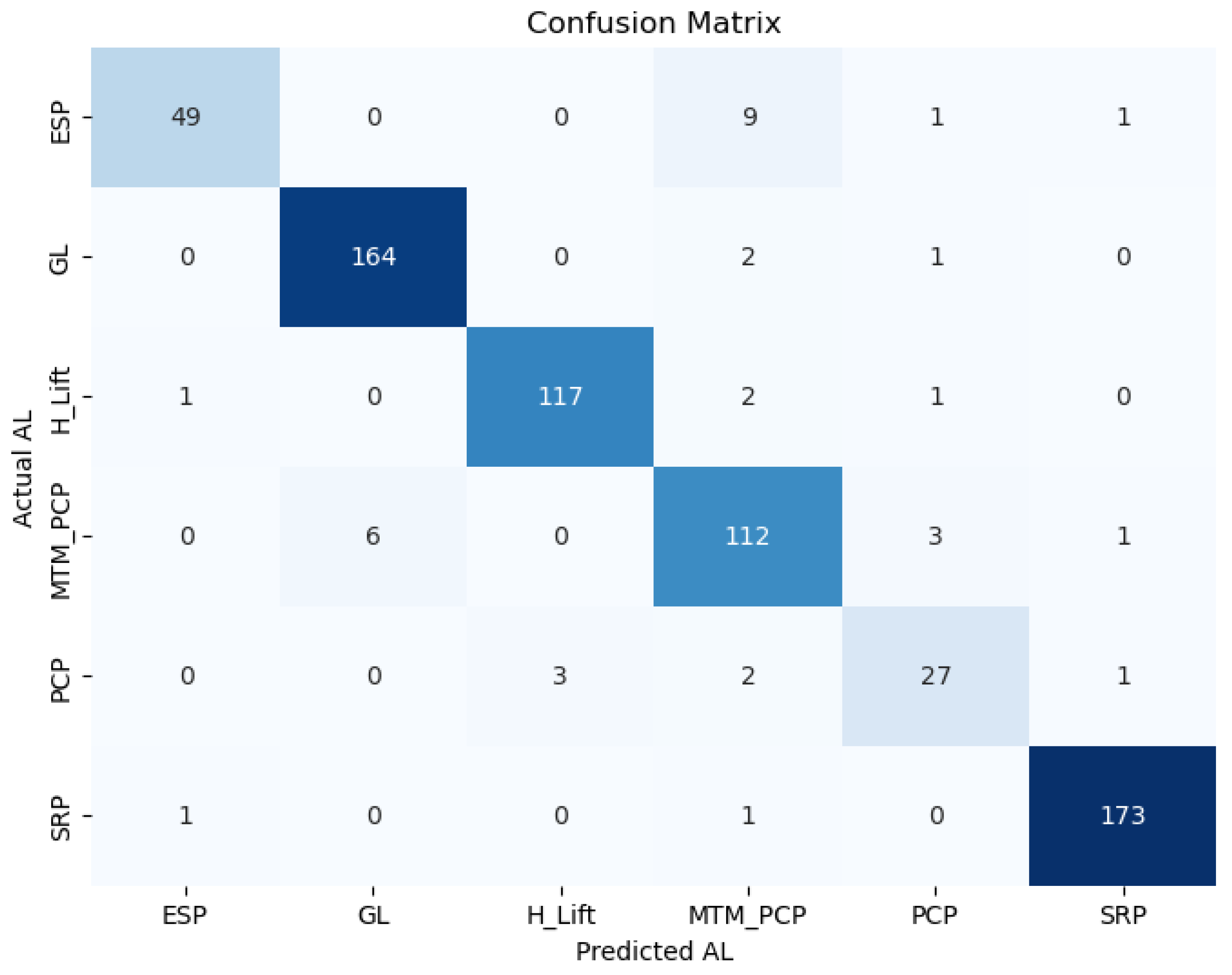
Figure 6 presents the confusion matrix, which provides a detailed breakdown of the model’s classification performance for each artificial lift (AL) method. The matrix compares actual versus predicted classifications, illustrating how well the model identifies each AL type. The diagonal elements represent correctly classified instances, showing that the model accurately predicted 49 out of 60 ESP cases, 164 out of 167 Gas Lift (GL) cases, and 173 out of 175 Sucker Rod Pump (SRP) cases. Similarly, the classification of Hydraulic Lift (H_Lift) and MTM_PCP was highly reliable, with 117 and 112 correct predictions, respectively. The results show that the model performs well in distinguishing between different AL methods. The high number of correct predictions reinforces the effectiveness of the stacking model in selecting the appropriate artificial lift method based on field production data.
Figure 7.
Plot of Model’s Confusion Matrix.
3.2.3. ROC AUC and PR AUC Analysis
The model's performance was also evaluated using both Receiver Operating Characteristic - Area Under the Curve (ROC AUC) and Precision-Recall Area Under the Curve (PR AUC) as shown in Figure 8. While ROC AUC provides an overall measure of separability, PR AUC is more informative for handling imbalanced datasets as it focuses on precision and recall.
The high ROC AUC scores (0.96–0.99) as shown in Table 3 indicate that the model is effective in distinguishing between different classes. However, the PR AUC values (0.87–0.97) reveal differences in the model's ability to maintain precision, particularly for the MTM_PCP class (PR AUC = 0.87). This suggests that while the model can correctly identify this class, it struggles with false positives when recall is high. The macro-average PR AUC of 0.9388 and micro-average PR AUC of 0.9449 further confirm that the model maintains strong overall performance, though precision varies across classes. Given the dataset's potential imbalance, PR AUC provides a more nuanced understanding of classification performance
3.3. Sensitivity Analysis
To interpret the contribution of each input feature to the model’s predictions, SHapley Additive exPlanations (SHAP) was employed. SHAP values quantify the impact of each feature on the model output, providing insights into their relative importance.
Figure 9 presents the SHAP summary plot, where the mean absolute SHAP values represent the average magnitude of each feature’s contribution. The results indicate that Daily Production Fluid (BLPD) has the highest impact on the model’s classification decisions, followed by Daily Gas Production (MSCF/D), Daily Oil Production (STB/D), and Daily Sand Production (RB/D). This suggests that production-related parameters play a crucial role in determining the classification outcome. Additionally, features such as Daily Water Production (BWPD) and Water Cut (%) exhibit moderate importance, while Wellhead Pressure (psi) and Gas-Oil Ratio (GOR, SCF/STB) have the least influence on the model's predictions. These findings align with the physical understanding of well performance, where production rates significantly affect operational conditions.
To further investigate how each feature affects individual Artificial Lift predictions, the SHAP beeswarm plot was generated. This plot (Figure 10) provides a detailed, instance-level visualization of feature importance and their impact on model predictions. Each point represents a single observation, with its position along the x-axis indicating the SHAP value, which quantifies the effect of a feature on the model’s output. Features are sorted by importance, with the most influential ones appearing at the top. The color gradient represents feature values, where red signifies higher values and blue represents lower values. A positive SHAP value suggests an increase in the predicted output, whereas a negative SHAP value indicates a decrease. By capturing the interactions between different features and their directional effects, the beeswarm plot enhances the interpretability of the model’s decision-making process. For the H_Lift model, the strong influence of daily produced fluid is reasonable, as hydraulic lift systems rely on fluid movement to generate the necessary pressure differential for lifting. A higher fluid rate generally enhances system efficiency, provided the pump is operating within its designed capacity. However, in practical applications, factors like fluid viscosity and sand content can introduce additional challenges, such as increased pressure losses or equipment wear. Similarly, for the Gas Lift model, the dominance of daily oil production aligns with expectations since gas lift is primarily optimized for oil output. However, water cut can significantly impact efficiency by increasing the hydrostatic column weight, thereby requiring more gas injection to sustain lift performance. Additionally, sand production being a key factor is reasonable, as sand can erode gas lift valves and create flow restrictions, although its impact depends on the effectiveness of sand control measures.
3.4. Comparison with Recent Literature
To contextualize the accuracy of our study, we compare our model's performance with two similar recent studies in machine learning – informed artificial lift selection. Figure 11 summarizes the accuracies reported in these studies alongside our findings. The results indicate that our stack model outperforms the accuracy reported in both Mohaned et al [1] and Ounsakul et al [4], demonstrating the robustness and effectiveness of our approach.
4. Conclusion
This study successfully developed and evaluated a machine learning-based approach for artificial lift selection using field production data. The stacked model achieved a high classification accuracy of 94.7%, outperforming models from previous studies. The confusion matrix and evaluation metrics confirmed that Sucker Rod Pump (SRP) and Gas Lift (GL) exhibited the highest predictive performance, while Progressive Cavity Pump (PCP) had the lowest due to data imbalance. SHAP sensitivity analysis revealed that daily fluid production, gas production, and oil production were the most influential parameters in lift selection. The findings align with operational expectations, reinforcing the critical role of production rates in artificial lift performance. The integration of machine learning in artificial lift selection enhances decision-making by providing data-driven insights, reducing reliance on heuristics, and improving efficiency. Future work could explore the integration of additional well parameters and optimization techniques to further refine predictive accuracy.
Funding
This research did not receive any specific grant from funding agencies in the public, commercial, or not-for-profit sectors.
References
- Mohaned Alhaj A. Mahdi, M. A. and G. O. An Artificial Lift Selection Approach Using Machine Learning . Energies 2023, 16, 2853. [Google Scholar] [CrossRef]
- Nguyen, H. T., & Del Mundo, F. C. (2016). Improving artificial lift design through dynamic simulation. Society of Petroleum Engineers - SPE North America Artificial Lift Conference and Exhibition 2016, (October), 25–27. [CrossRef]
- Nosakhare, A., Igemhokhai, S., Aimhanesi, S., Ugbodu, F., & Iyore, N. (2024). Heliyon Data-driven intelligent modeling , optimization , and global sensitivity analysis of a xanthan gum biosynthesis process. Heliyon, 10(3), e25432. [CrossRef]
- Ounsakul, T., Sirirattanachatchawan, T., Pattarachupong, W., Yokrat, Y., & Ekkawong, P. (2019). Artificial lift selection using machine learning. International Petroleum Technology Conference 2019, IPTC 2019, (June). [CrossRef]
- Shi, J., Chen, S., Zhang, X., Zhao, R., Liu, Z., Liu, M., et al. (2019). Artificial lift methods optimising and selecting based on big data analysis technology. International Petroleum Technology Conference 2019, IPTC 2019. [CrossRef]
- Speiser, J. L., Miller, M. E., Tooze, J., & Ip, E. (2019). A comparison of random forest variable selection methods for classification prediction modeling. Expert Systems with Applications, 134, 93–101. [CrossRef]
- Akosa, J. Predictive accuracy: A misleading performance measure for highly imbalanced data. Proc. SAS Glob. Forum 2017, 12, 942. [Google Scholar]
- Tan, P.N.; Steinbach, M.; Kumar, V. Classification: Basic concepts, decision trees, and model evaluation. Introd. Data Min. 2006, 1, 145–205. [Google Scholar]
- Alshboul, O., Shehadeh, A., Almasabha, G., & Almuflih, A. S. (2022). Extreme Gradient Boosting-Based Machine Learning Approach for Green Building Cost Prediction. Sustainability, 14(11), 6651. [CrossRef]
- Shapley, L. (1997). 7. A Value for n-Person Games. Contributions to the Theory of Games II (1953) 307-317.. In H. Kuhn (Ed.), Classics in Game Theory (pp. 69-79). Princeton: Princeton University Press. [CrossRef]
- Štrumbelj, E., & Kononenko, I. (2014). Explaining prediction models and individual predictions with feature contributions. Knowledge and Information Systems, 41(3), 647–665. [CrossRef]
- Rahmawati, S. D., Chandra, S., Aziz, P. A., et al. Integratedapplication of flow pattern map for long-term gas liftoptimization: A case study of Well T in Indonesia. Jour-nal of Petroleum Exploration and Production Technology,2020, 10(4): 1635-1641.
- Wood, D. A. Gamma-ray log derivative and volatility attributesassist facies characterization in clastic sedimentary se-quences for formulaic and machine learning analysis.Advances in Geo-Energy Research, 2022, 6(1): 69-85.
- Yavari, H., Khosravanian, R., Wood, D. A., et al. Applicationof mathematical and machine learning models to predictdifferential pressure of autonomous downhole inflow con-trol devices. Advances in Geo-Energy Research, 2021,5(4): 386-406.
- Mahdiani, M. R., Khamehchi, E., Hajirezaie, S., et al. Mod-eling viscosity of crude oil using k-nearest neighbor al-gorithm. Advances in Geo-Energy Research, 2020, 4(4):435-447.
- Choubey, S., Karmakar, G. P. Artificial intelligence techniquesand their application in oil and gas industry. Artificial In-telligence Review, 2021, 54(5): 3665-3683.
- M. Ali, R. Prasad, Y. Xiang, Z.M. Yaseen, Complete ensemble empirical mode decomposition hybridized with random forest and kernel ridge regression model for monthly rainfall forecasts, J. Hydrol. 584 (2020) 124647. [CrossRef]
- Brownlee, J. Data Preparation for Machine Learning: Data Cleaning, Feature Selection, and Data Transforms in Python; Machine Learning Mastery: Vermont, Australia, 2020. [Google Scholar]
- Bravo, C., Saputelli, L., Rivas, F., et al. State of the artof artificial intelligence and predictive analytics in theE&P industry: A technology survey. SPE Journal, 2014b,19(4): 547-563.
- Fern ́andez, A., Garc ́ıa, S., Galar, M., et al. Introduction toKDD and Data science, in Learning From Imbalanced Data Sets, edited by A. Fern ́andez, S. Garc ́ıa, M. Galar,et al., Springer, Berlin, pp. 1-16, 2018.
- Silla, C. N., Freitas, A. A. A survey of hierarchical classifi-cation across different application domains. Data Miningand Knowledge Discovery, 2011, 22, 31-72.
- De Carvalho, A. C. P., Freitas, A. A. A tutorial on multi-label classification techniques, in Foundations of Com-putational Intelligence, edited by A. Abraham., A. E.Hassanien, and V. Sn ́aˇsel, Berlin Heidelberg, Germany,pp. 177-195, 2009. 2009.
- Wolpert, D. H. (1992). Stacked generalization. Neural Networks, 5(2), 241-259. [CrossRef]
- Molnar, C. (2020). Interpretable machine learning. Lulu. com.
Figure 1.
Distribution plot of the features in the dataset.
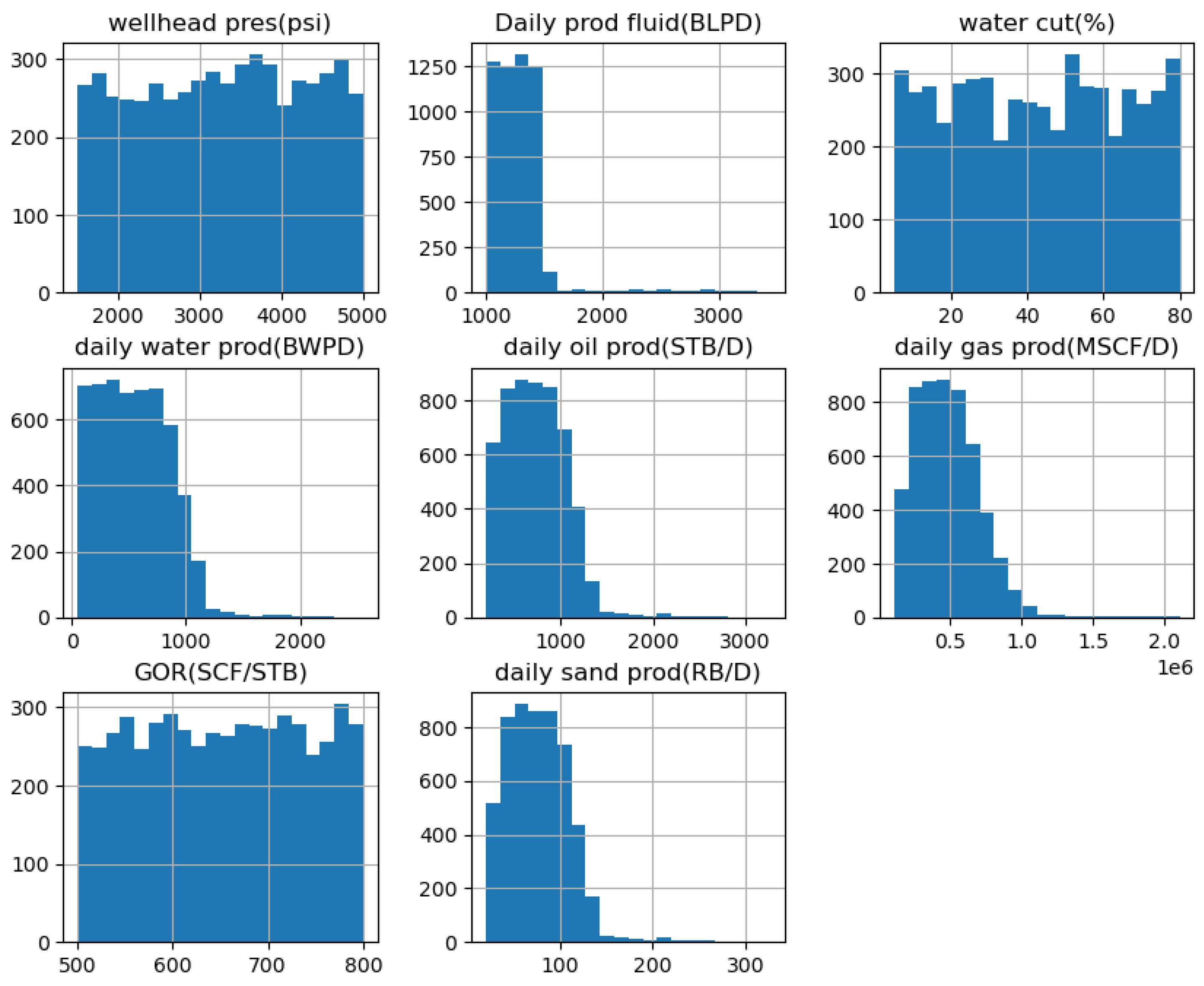
Figure 2.
Pearson Correlation between numerical features in the data.
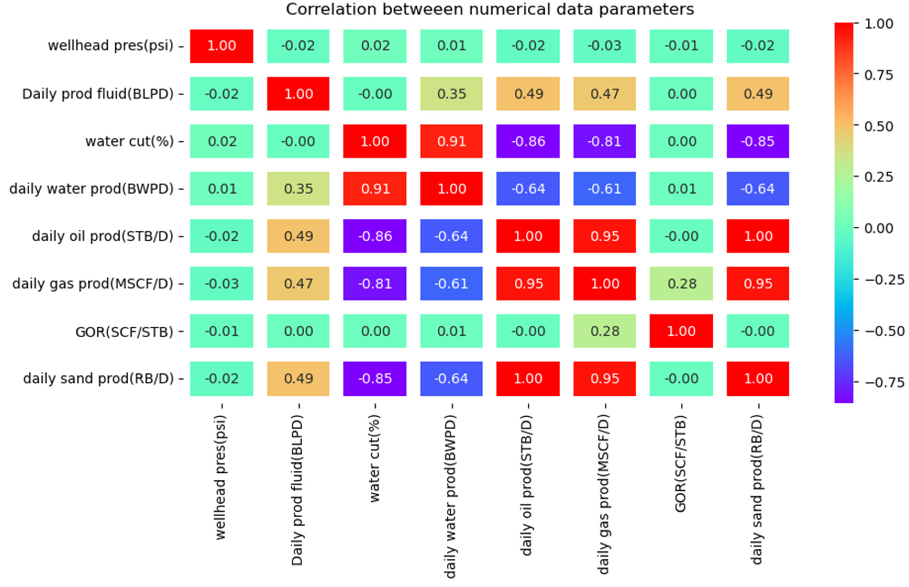
Figure 3.
Artificial Lift distribution in the dataset.
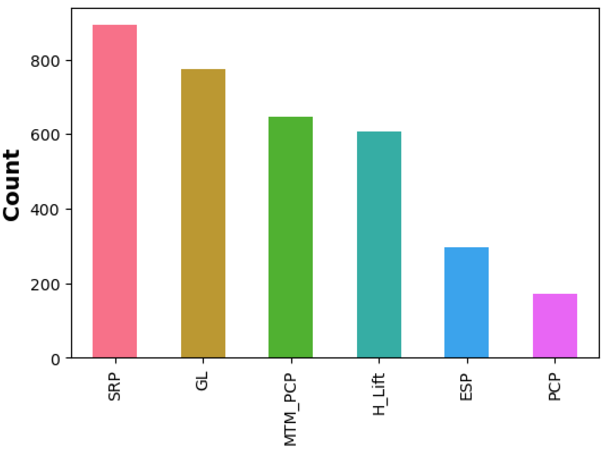
Figure 4.
Cumulative oil production by Artificial Lift.
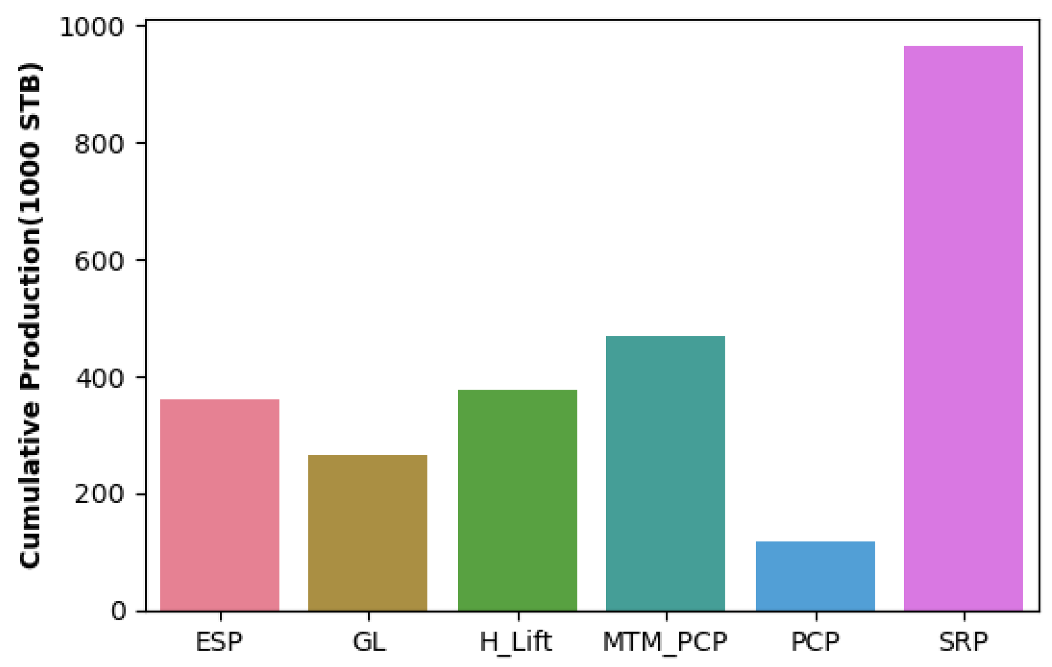
Figure 6.
The implemented stack model.
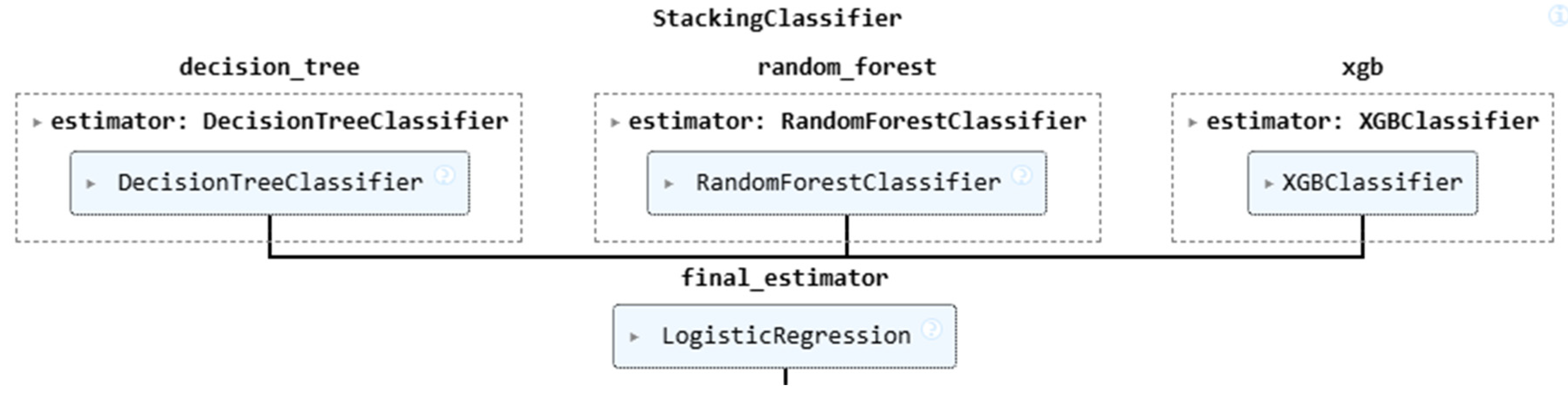
Figure 8.
Multiclass (a) ROC curve of the stack model (b) PR curve of the stack model.
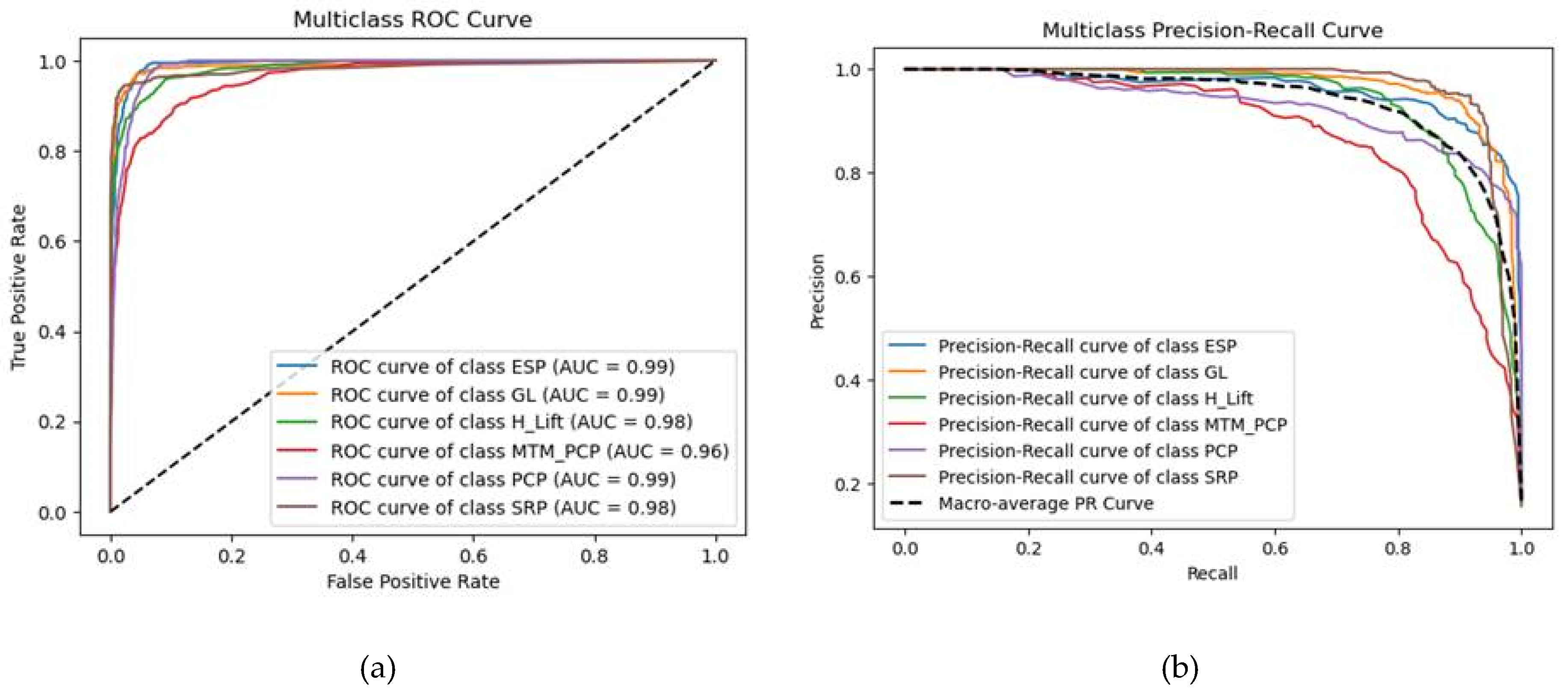
Figure 9.
SHAP Sensitivity plot of the Features in Predicting Artificial Lift Method.
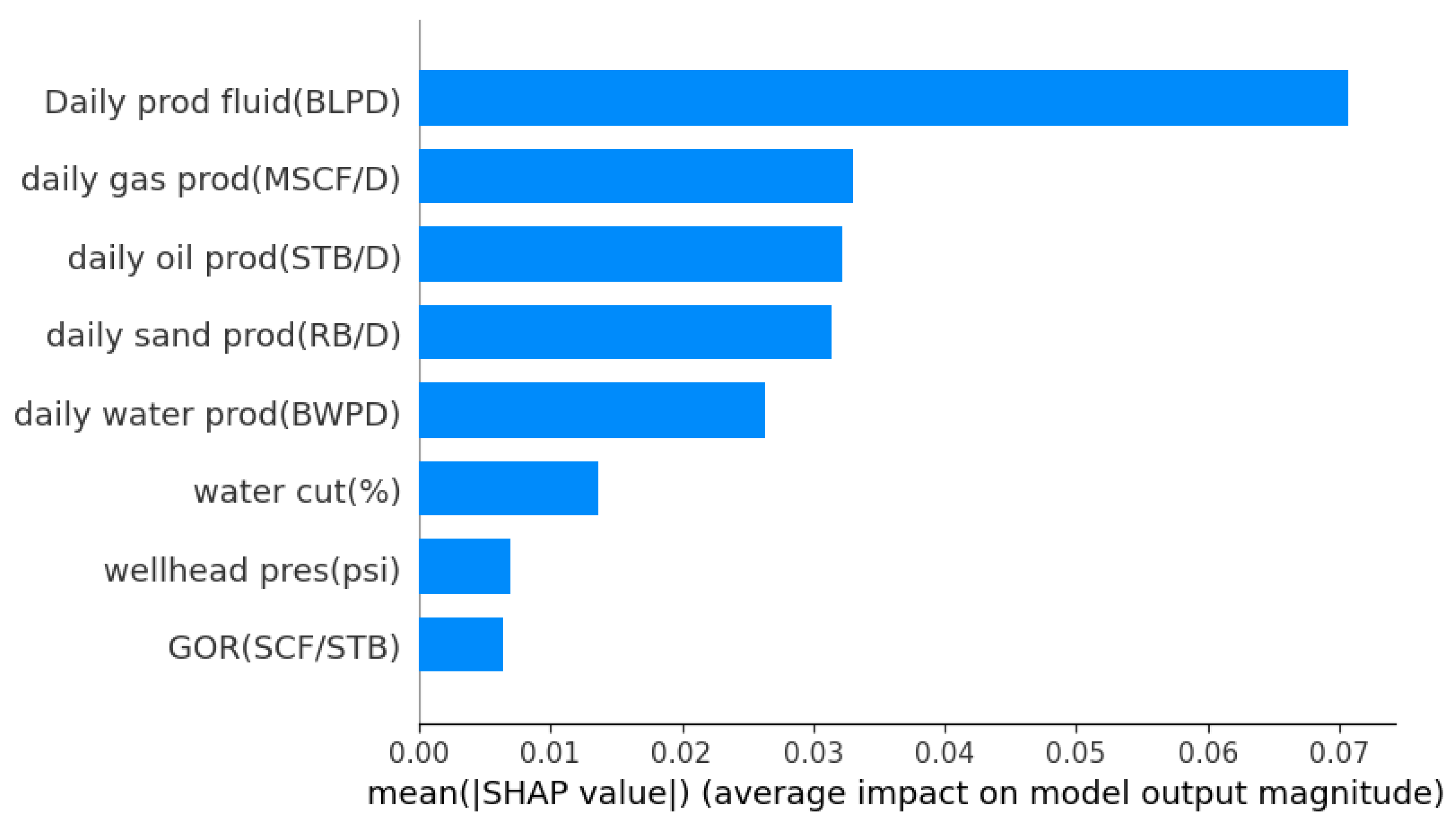
Figure 10.
SHAP Sensitivity plot for (a) ESP (b) GL (c) HL (d) MTM_PCP (e) PCP (f) SRP.
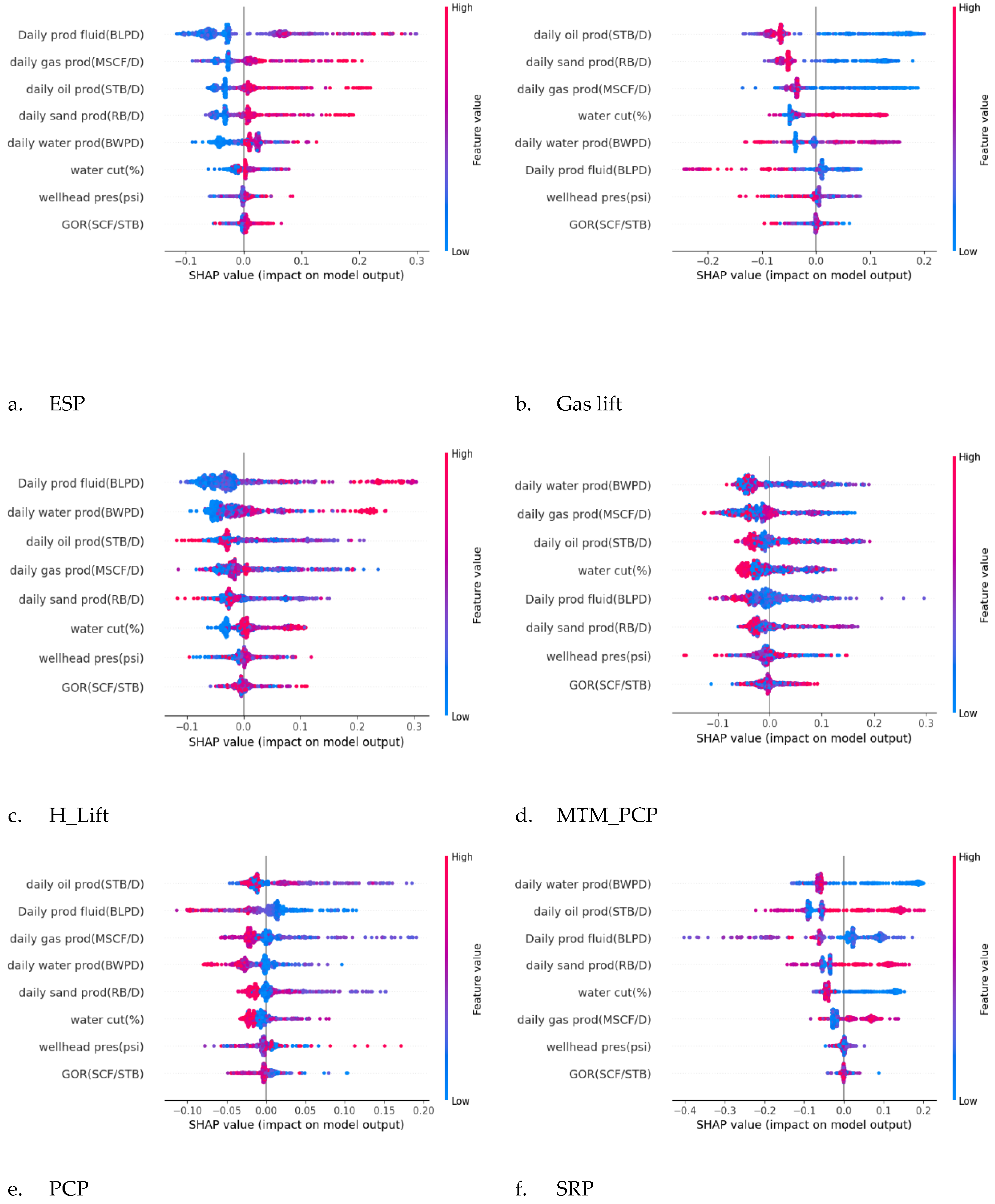
Figure 11.
Model’s Comparison of accuracy with relevant studies.
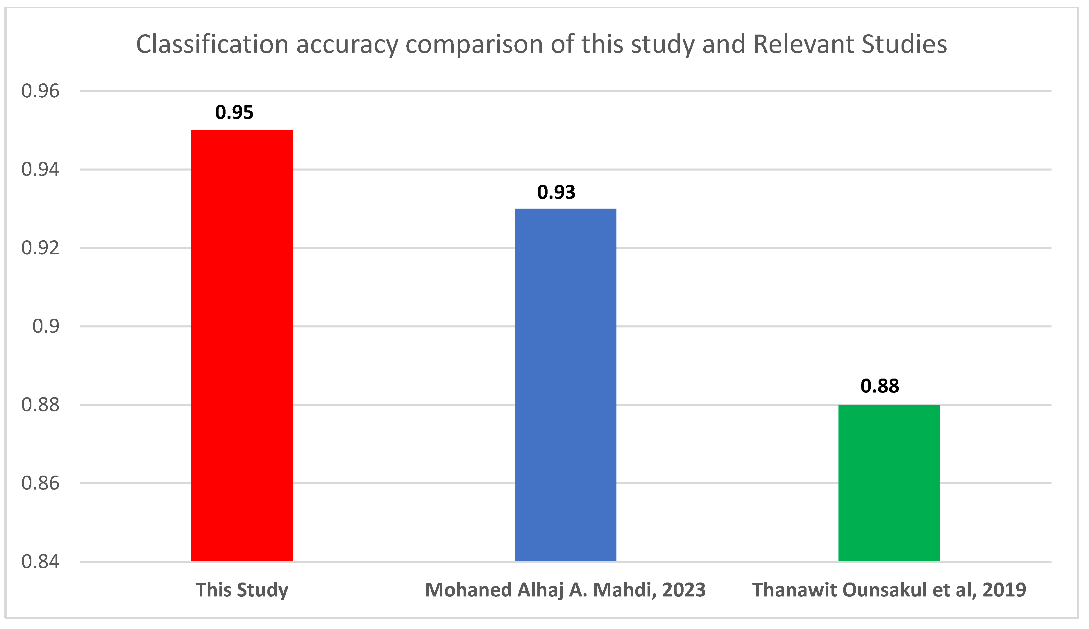

Table 1.
Optimal Hyperparameters for the utilised ML models.
| Model | Hyperparameters | Final Optimized value |
|---|---|---|
| DT | max_depth | 5 |
| min_samples_split | 2 | |
| random_state | 9 | |
| RF | n estimators | 500 |
| max depth | 5 | |
| max features | 3 | |
| random_state | 9 | |
| XGB | max depth | 5 |
| gamma | 0.01 | |
| n estimators | 500 | |
| subsample | 1 | |
| random state | 9 |
Table 2.
Stacked Model’s Classification Report.
| precision | recall | f1-score | support | |
|---|---|---|---|---|
| ESP | 0.960784 | 0.816667 | 0.882883 | 60 |
| GL | 0.964706 | 0.982036 | 0.973294 | 167 |
| H_Lift | 0.975 | 0.966942 | 0.970954 | 121 |
| MTM_PCP | 0.875 | 0.918033 | 0.896 | 122 |
| PCP | 0.818182 | 0.818182 | 0.818182 | 33 |
| SRP | 0.982955 | 0.988571 | 0.985755 | 175 |
| accuracy | 0.946903 | 0.946903 | 0.946903 | 0.946903 |
| macro avg | 0.929438 | 0.915072 | 0.921178 | 678 |
| weighted avg | 0.947633 | 0.946903 | 0.946634 | 678 |
Table 3.
ROC UAC and PR AUC values.
| Class | ROC AUC | PR AUC |
|---|---|---|
| ESP | 0.99 | 0.9593 |
| GL | 0.99 | 0.9674 |
| H_Lift | 0.98 | 0.9397 |
| MTM_PCP | 0.96 | 0.8741 |
| PCP | 0.99 | 0.9272 |
| SRP | 0.98 | 0.9651 |
| Macro-Average | - | 0.9388 |
| Micro-Average | - | 0.9449 |
Disclaimer/Publisher’s Note: The statements, opinions and data contained in all publications are solely those of the individual author(s) and contributor(s) and not of MDPI and/or the editor(s). MDPI and/or the editor(s) disclaim responsibility for any injury to people or property resulting from any ideas, methods, instructions or products referred to in the content. |
© 2025 by the authors. Licensee MDPI, Basel, Switzerland. This article is an open access article distributed under the terms and conditions of the Creative Commons Attribution (CC BY) license (http://creativecommons.org/licenses/by/4.0/).
Copyright: This open access article is published under a Creative Commons CC BY 4.0 license, which permit the free download, distribution, and reuse, provided that the author and preprint are cited in any reuse.


