Submitted:
25 April 2024
Posted:
30 April 2024
You are already at the latest version
Abstract
Over the past decade, the volume and quality of data in the oil and gas industry have exploded, breeding exciting opportunities to implement machine learning for better data- driven decisions. One critical example is hydraulic fracturing (HF), given our ever-growing reliance on HF to meet global hydrocarbon demand. This paper systematically explores the work of several researchers to apply ML techniques (including linear regression, neural networks, support vector machine, decision trees, and more) to HF-related operations, from production forecast to HF design. Furthermore, this study examines how optimization algorithms (including gradient-free, differential evolution, and surrogate-based optimizations) are incorporated with different ML techniques for selecting optimal HF parameters (like fracture number, proppant concentration, and more) during the planning process. The paper aims to provide a comprehensive overview without delving too deeply into technical intricacies to ensure accessibility for a broader audience. Additionally, it introduces innovative techniques currently being integrated into the industry and offers a clear understanding of the processes involved. Ultimately, the analysis concludes that machine learning is an accurate and cost-effective alternative for hydraulic fracturing optimization.
Keywords:
Machine learning
; artificial intelligence
; hydraulic fracturing
; hyperparameter optimization
; shale
; operational factors.
Introduction
Despite significant efforts to transition to renewable energy sources, the reality is that fossil fuels still account for 80% of the world’s energy supply (bp, 2022). Given the ever-growing need for energy independence, many researchers agree that fossil fuels will be crucial in the energy transition journey over the coming decades (Chishti et al., 2023; Razzaq et al., 2023). Hence, hydrocarbon production optimization is of significant interest.
Hydraulic fracturing is one such optimization technique. Moreover, over the past decade, hydraulic fracturing technology has notably increased within unconventional reservoir development (Zhiwei Wang et al., 2023). This advancement has primarily manifested in its application in horizontal wells to extract shale gas, tight gas, and oil reservoirs. This surge in hydraulic fracturing activity has been particularly notable in China, Russia, and North America. For example, the US Energy Department stipulates that about 95% of new wells drilled today in the US are hydraulically fractured. According to Cook, Perrin and Wagener (2018), this contributes about two-thirds of natural gas and 50% of US crude oil production. Given the importance of hydraulic fracturing, several techniques are used to optimize the process, including reservoir simulations, decline curve analysis, hydraulic fracturing modeling, and rate transient analysis (Syed et al., 2022). However, these techniques have limited accuracy.
Interestingly, significant development in data analysis has led to the emergence of more sophisticated and efficient algorithms designed for the interpretation and identification of data patterns, as well as the refinement of algorithmic models - commonly called Machine Learning (ML) and Artificial Intelligence (AI). ML and AI have transformed every industry, enabling the more effective utilization and comprehension of vast datasets. The upstream sector of the oil and gas sector is no exception. The application of Machine Learning provides a powerful tool for decision-making processes spanning from exploration endeavors to the management of field development (Agbaji, 2021).
With vast datasets arising from the wide-scale adoption of hydraulic fracturing, these advanced computational techniques offer significant potential for optimizing the hydraulic fracturing process. ML algorithms, when trained on large datasets comprising geological and operational parameters and combined with several optimization techniques (like gradient- free, evolutionary, and surrogate-based algorithms), can enhance the predictive modeling of fracture propagation, aiding in the optimization of well placement and hydraulic fracturing designs (Sprunger et al., 2022). Moreover, AI-driven systems enable real-time monitoring and control of hydraulic fracturing operations, allowing for immediate adjustments to wellbore conditions, thereby improving overall efficiency and reducing operational and environmental risks associated with the process (LEI et al., 2022).
This paper provides a thorough analysis of several novel integrations of ML and optimization algorithms into hydraulic fracturing practices as part of the ongoing evolution of the oil and gas industry towards data-driven decision-making and enhanced operational efficiency.
Methodology
Research on ML/AI applications in hydraulic fracturing has skyrocketed over the past decade. This paper thematically explores the recent and crucial advances in this research area. First, a good insight into hydraulic fracturing and its significant challenges are highlighted before examining some influential machine learning and optimization techniques. We then explore several case studies to show how ML/AI can be applied for hydraulic fracturing optimization. Finally, we examine and track some possible future trends in this exciting field.
Hydraulic Fracturing Overview
The fundamental concept behind HF involves the injection of high-pressure fluids, along with proppant particles, into wells to create fractures within the reservoir formation, facilitating the flow of hydrocarbons to the surface. One of the remarkable advancements in HF technology over the last two decades has been the transition to directional drilling and multistage fractured completions. This evolution has enabled the development of unconventional reservoirs more efficiently and effectively. However, as HF technology has become more complex, challenges have arisen from technical complexities, environmental concerns, optimization, and economic considerations.
Technical Challenges
One of the foremost challenges in hydraulic fracturing is the inherent heterogeneity of reservoirs. Subsurface formations often exhibit variations in porosity, permeability, and stress regimes. These reservoir heterogeneities can significantly impact fracture propagation and the ultimate production from HF operations (Vishkai and Gates, 2019). Geomechanical parameters, such as brittleness index and stress magnitude, influence fracture growth and must be carefully considered in fracture design to optimize production (Lu, Jiang, Qu, et al., 2022).
HF design remains a complex process involving determining optimal parameters like the fracturing stages number, fracturing fluid volume, perforating clusters, and proppant concentration. Suboptimal designs can lead to underperforming wells, with up to 30% of fractures in multistage completions failing to contribute to production (Al-Shamma et al., 2014; He et al., 2017). The reasons for such design flaws range from reservoir heterogeneity to insufficiently optimized pumping schedules.
Reservoir numerical simulation, a common approach for HF design, relies on coupled solid- fluid mechanics models to evaluate fracture parameters. Zhao et al. (2019) adopted a 3D discrete fracture model (DFM) for HF characterization and oil production geometry. Fu et al. (2020) simulated hydraulic fracture propagation with an unconventional fracture model (UFM), maximizing oil production by optimizing segments and cluster spacing. Using Petrel, Lu et al. (2022) optimized cluster spacing, stage length, and fracturing fluid volume under varying reservoir conditions. While these simulations are valuable, they often entail time- consuming and computationally intensive processes, especially when considering reservoir heterogeneity (Zheng et al., 2020). Furthermore, they may need to fully account for the impacts of fracturing fluid and proppant on induced fractures, limiting their accuracy in design optimization.
Environmental Concerns
One of the primary concerns is the potential contamination of groundwater sources. Numerous studies have documented methane migration into drinking water supplies near fracking operations (Osborn et al., 2011; Jackson et al., 2013), which can pose serious health risks and contribute to greenhouse gas emissions. HF is also associated with induced seismicity. The high-pressure injection of fluids can trigger earthquakes, particularly in regions with pre-existing fault systems (Spellman, 2012). Mitigating the risk of induced seismic events while maximizing production is a complex challenge that requires careful monitoring and regulation. That is why adequate HF design is paramount, and ML can aid with that.
Optimization Dilemmas
Optimizing hydraulic fracturing parameters – from cluster spacing to stage length, fracturing fluid volume, and proppant concentration – is essential for maximizing production. Various HF simulators like P3D, PKN, and KGD are used for this. Detournay (2016) details several models used to construct the objective function for this optimization problem. However, determining the optimal values for these parameters remains a complex and time-consuming task. Traditional parametric-sensitivity analysis often fails to achieve global optimal designs (Detournay, 2016; Wang and Chen, 2019).
When it comes to HF, the balancing act between incremental future revenue and execution costs poses a significant optimization challenge. There is limited research on incorporating cost implications (like net present value - NPV) into fracture parameter optimization (Duplyakov et al., 2022).
ML/AI for HF Overview
ML is gaining prominence in the petroleum industry because it allows for fast and efficient analysis of vast datasets being generated. ML is better than traditional techniques because it can automatically learn and adapt from data and extract convoluted patterns and links that may be difficult to determine using predetermined rules. Coupled with its extensive scalability capabilities, ML offers great promise in the field of hydraulic fracturing.
Several researchers have adopted different ML algorithms to solve several critical challenges in hydraulic fracturing. Most work employ ML to predict the production profile and cumulative production after a fracturing job (Temizel et al., 2015; Schuetter et al., 2018; Alarifi and Miskimins, 2021; Ibrahim, Alarifi and Elkatatny, 2022; Sprunger et al., 2022; Syed et al., 2022). Others adopt ML to determine the inverse problem of determining the optimal hydraulic fracturing parameters given a desired production output (Duplyakov et al., 2022; Sprunger et al., 2022). Such parameters include proppant and fluid volumes, fracture length, number of HF stages, and pump rates. Some researchers have even incorporated economic objective functions in the HF optimization process (Dong et al., 2022; Lu, Jiang, Yang, et al., 2022). The integration of these goals is described in Figure 1. This section briefly describes some of the most used ML algorithms in hydraulic fracture optimization.
Production-Prediction Models
From the literature, the most common ML models for predicting production rate/cumulative production after a fracking job include artificial neural network (ANN), Random Forest (RF) regression, support vector machine (SVM), and decision trees.
Multilayer Perceptron (MLP)
MLPs, which are also known as artificial neural networks (ANNs), are modeled after the information-processing mechanisms found in human neurons. They offer an abstract mathematical framework characterized by distributed parallel information processing and adaptive dynamics involving numerous interconnected basic neurons. This approach closely resembles the way the human brain processes information, where neurons interact with one another, knowledge is encoded in neuron weights, and the processes of learning and recognition depend on the changing coefficients of these weights.
In hydraulic fracturing optimization, MLPs are instrumental in modeling the intricate relationships between various operational parameters and production outcomes, allowing for highly accurate and adaptable predictions. A typical MLP neural network configuration consists of input, hidden, and output layers, where each neuron represents a processing unit (Figure 2). During training, the network learns and adjusts the connection weights (representing the synaptic strength between neurons) to optimize predictive accuracy (Haykin, 2009).
The following equations define the mathematical model of a single neuron in an MLP:
where x and y represent the inputs and outputs, respectively. W, b, and σ are the weights, biases, and the activation function, respectively.
{ 𝑦̂ = 𝑓𝑛 (𝑓𝑛−1 (… 𝑓1(𝑥))) ,
𝑓𝑛(𝑥) = 𝜎𝑛(𝑊𝑛𝑥 + 𝑏𝑛)
Gradient Boosted Decision Tree
GBDT is characterized by its ability to progressively reduce learning errors throughout training, making it particularly advantageous when faced with imbalances in actual production data. Its robustness to outliers and capacity to handle continuous and discrete data forms further underscore its suitability for hydraulic fracturing applications.
At the core of the GBDT algorithm lies an ensemble of decision trees, each designed to correct the errors or residuals of its predecessors. This iterative process ensures that the model focuses on areas where prior predictions fell short, progressively enhancing the accuracy of production forecasts. The primary concept driving GBDT is to train each new learner in the gradient direction to minimize the learning error of the previous learner, effectively building upon the previous model (Sun et al., 2020).
Mathematically, the ensemble of decision trees in GBDT can be expressed as:
where 𝐹(𝑚−1)(𝑥) is the combination of the first m-1 decision trees and 𝑓𝑖(𝑥) represents an individual decision tree. The gradient of the loss function 𝑔𝑚(𝑥) guides the learning process, and each new decision tree (𝑓𝑚(𝑥)) is estimated by minimizing the gradient error:
𝑚−1
𝐹(𝑚−1)(𝑥) = ∑ 𝑓𝑖(𝑥)
𝑖=0
𝑓𝑚(𝑥) = −𝜌𝑚𝑔𝑚(𝑥)
𝜌𝑚 is the learning step, which defines the rate at which the model adapts and improves.
Random Forest
As seen in Figure 3, RF employs an ensemble of decision trees constructed with random data and feature subsets during training. The process of leveraging several decision trees is called "bagging." This stochastic process mitigates overfitting, a standard modeling challenge. The ensemble combines individual tree predictions to generate a robust final output.
Mathematically, suppose the set of regression trees is given as {ℎ(𝑋, 𝜃𝑘), 𝑘=1,2,3,⋯}. In that case, the final prediction is obtained by averaging the predictions of these trees for a given sample, resulting in improved accuracy and reduced variance. The mean squared random error is typically minimized in RF. As the number of trees (k) increases infinitely, the RF regression function converges to the expected value of the predictions (Gamal et al., 2021).
Gradient Boosted Machine (BGM)
GBM is a powerful machine learning technique widely applied in hydraulic fracturing optimization for production prediction. Unlike Random Forest (RF), GBM sequentially builds a decision tree ensemble (Bahaloo, Mehrizadeh and Najafi-Marghmaleki, 2023). Each tree corrects errors made by its predecessors, emphasizing areas where earlier trees underperformed. This iterative process results in a final model resembling a linear regression model with numerous terms, each representing a tree. GBM captures complex relationships among input parameters, making it invaluable for accurately predicting hydraulic fracturing production levels (Syed et al., 2022).
GBM's adaptability and capacity to handle noisy and high-dimensional data are advantageous in optimizing hydraulic fracturing operations, where intricate interactions significantly influence production outcomes.
Support Vector Machine
SVM is renowned for handling high-dimensional datasets, capturing complex or non-linear relationships, and providing robust predictions. SVM operates by identifying a hyperplane that optimally separates data points into distinct classes or, in regression tasks, predicts a continuous target variable while maximizing the margin between the data points and the hyperplane. This margin optimization ensures that SVM generalizes well to unseen data, contributing to its predictive accuracy.
Fracturing Parameters Optimization
In recent years, different algorithms have also been applied to determine the optimum fracturing parameters and NPV - ranging from gradient-free optimization methods to surrogate-based optimization and evolutionary optimization techniques.
Gradient-Free Optimization Methods
Gradient-free optimization methods have gained prominence in hydraulic fracturing optimization due to their ability to handle complex, non-convex objective functions without requiring gradient information. These methods explore the parameter space through a sequence of function evaluations, seeking to find the global optimum. Popular algorithms in this category include Genetic Algorithms, Particle Swarm Optimisation (PSO), and Nelder- Mead. In hydraulic fracturing, where the objective function often lacks analytical gradients due to the complex physics involved, gradient-free methods offer an advantageous approach for optimizing parameters such as fluid injection rates, proppant concentrations, and well placement (Jones, Schonlau and Welch, 1998).
Evolutionary Optimization Techniques
Evolutionary algorithms (EAs) are a subset of gradient-free optimization. EAs draw inspiration from the principles of biological evolution and natural selection. Algorithms such as Genetic Algorithms and Differential Evolution work by adapting a population of potential solutions over generations (Deb et al., 2000). Mimicking the traits of a flock of birds or a swarm of particles, the Particle Swarm Optimisation (PSO) algorithm balances personal and global exploration to explore the search space efficiently and converge towards the optimal solution (Clerc, 2010). Hydraulic fracturing optimization problems can be cast as evolutionary processes where solutions that exhibit desirable traits (e.g., higher fracture propagation or increased reservoir contact) are selected and reproduced. These techniques effectively explore large solution spaces and can handle multi-objective optimization problems.
Surrogate-Based Optimization
Surrogate-based optimization techniques leverage the construction of surrogate models (e.g., Gaussian Process Regression or Radial Basis Functions) to approximate the expensive objective function. These surrogate models are iteratively updated and optimized, which reduces the number of costly simulations or experiments required to find optimal fracturing parameters (Forrester, Sobester and Keane, 2008). In hydraulic fracturing applications, where simulation runs can be computationally intensive, surrogate-based optimization techniques have demonstrated efficiency and accuracy (Xiao et al., 2022). They are instrumental when dealing with noisy or uncertain objective functions.
ML Challenges
When using ML algorithms, there are several important considerations to ensure the resulting models are accurate and scalable. Some of these include:
Overfitting
Overfitting describes a phenomenon when a machine learning model fits the training data by capturing noise and peripheral patterns. In hydraulic fracturing optimization, overfit models may not generalize well to unseen data, potentially leading to poor performance in real-world scenarios. For example, Alimkhanov and Samoylova (2014) employed 178 features with just 289 well data. Given that the features outnumber the available training data set, any resulting model is likely to overfit the data - consequently resulting in poor generalization evidenced by a wide range of coefficient of determination from 0.2 to 0.6 Techniques such as regularisation (e.g., L1 or L2 regularisation), cross-validation, and the use of less susceptible ML algorithms are essential to mitigate overfitting (Hastie et al., 2009).
Dimensionality Reduction
High-dimensional feature spaces can introduce computational challenges and hinder model interpretability. Dimensionality reduction is accomplished with methods like t-distributed Stochastic Neighbor Embedding (t-SNE) or Principal Component Analysis (PCA). They can help extract meaningful information from data while reducing dimensionality. Applying these techniques can enhance the efficiency of hydraulic fracturing optimization models (Jolliffe, 2005).
Feature Importance Analysis
Identifying the most influential features in hydraulic fracturing optimization is critical for understanding the underlying processes. Techniques like feature importance scores, recursive feature elimination, or SHAP (SHapley Additive exPlanations) values can highlight which features contribute most significantly to model predictions (Lundberg, Erion and Lee, 2018). This analysis aids in decision-making and feature selection.
Hyperparameter Search
Proper selection of hyperparameters, such as learning rates, regularisation strengths, and model architectures, significantly impacts model efficacy. Methods like random search, grid search, or Bayesian optimization can methodically examine hyperparameter spaces and optimize hydraulic fracturing models (Bergstra and Bengio, 2012).
Uncertainty Quantification
Hydraulic fracturing optimization often involves uncertainty, including subsurface properties and measurement errors. Uncertainty quantification techniques, such as probabilistic modeling and Bayesian inference, can help gauge the reliability of model predictions and assist in risk assessment.
Production Prediction via ML
The primary goal of HF is production optimization. Hence, for every HF job, the vital question of projected production must be answered as the first part of the equation. Only then can the inverse problem of optimizing fracking parameters for optimal production be solved. This section examines the work of different researchers to answer the first question using ML techniques.
Morozov et al. (2020) address this problem using a data-driven approach. This study built a vast digital database of over ~20 oilfields (~6000 wells) in Western Siberia, Russia. This data consisted of a vector of 92 input variables, including reservoir geometry, fracturing parameters, and production data, where available. Extensive data cleaning was required with over 5000 data points (significantly more than other studies). Collaborative filtering was used to resolve missing data, while the t-SNE algorithm was used to spot irrelevant outliers. The CatBoost algorithm was used for production forecasts because, from the literature, it performs better than other boosting algorithms.
To avoid the problem of overfitting, feature analysis was performed to select the most crucial input variables, and OVAT analysis was used for feature selection, with the number of HF stages, total volume of injected fluid, and proppant per perforation interval being the most important factors affecting production forecast (Figure 5a). L2 regularisation was used to find the optimal hyperparameters summarised in Table 7. The CatBoost algorithm attained a coefficient of determination (R2) of 0.815 on the test set (Figure 5b).
Artificial Neural Network is also a widely used algorithm for production forecasts after HF. A study by Lu, Jiang, Yang, et al. (2022) developed a deep neural network for production forecast in a shale oilfield in Jimusar Sag and Xinjiang, China, after 1 year and 5 years. The dataset was created using 841 numerical simulation data as the training set in the Petrel environment. The numerical simulation used geological, geomechanical, completion, and fracturing parameters. Figure 6 shows the process for this modeling. 97 field data was used for the test set.
Moreover, this study built extensive data consisting of three kinds of data: well data (wellbore direction, location, and lateral length); formation data (porosity, oil saturation, thickness, horizontal stress, Poisson ratio, etc.); and completion data (cluster number, stage number, proppant, amount, fracturing fluid volume, proppant size, and volume). Reservoir sweet spot mapping was identified in a previous study by the author and categorized into type I (good), type II (moderate), and type III (poor). Table 1 summarizes the range of values for the parameters used in database building. Fine-tuning of the DNN model resulted in an optimized hyperparameters of 0.003 for learning rate, a ReLU activation function, 3 hidden layers, and 150 neurons in each layer.
The dataset was split into 673 samples for training, 168 for cross validation, and 87 for testing. The model performance showed that after 1 year, R2 on the test set was 0.81, while it was 0.83 after 5 years. Table 2 summarizes the evaluation criteria (mean average error (MAE), mean square error (MSE), and R2) of all data sets.
This study also compared the 1-year post-production using other ML algorithms (Random Forest and Support vector Machine) for completeness, and the results are summarized in Table 3. With lower MAE and MSE and a higher R2 across the training, validation, and test sets, DNN outperforms RF and SVM.
Ibrahim et al. (2022) collected production and completion data across 200 wells across the Niobrara shale formation in North America to estimate the EUR by applying two ML techniques (ANN and Random Forest). EUR is defined as total production until well abandonment. Key input parameters used include stage count, horizontal length (ft), TVD (ft), max treatment pressure (psi), total proppant volume, and total fluid volume (bbl). Initial attempts to predict EUR using RF resulted in a wide R2 discrepancy between the training and test set (0.93 vs. 0.79) (Figure 7a). This points to underfitting, necessitating the inclusion of other features for better model performance. The initial Qi was selected because of its importance in decline curve analysis (DCA). Random Forest gave good predictions for Qi with R2 of 0.98 and 0.95 for the train and test sets, respectively. Thereafter, predicting the EUR (with Qi included as an input feature) resulted in train and test R2 of 0.99 and 0.93, respectively (Figure 7b).
A similar experiment was conducted using ANN instead of RF and with Qi included as an input parameter. ANN also showed even better production predictive capabilities with R2 of 0.96 and 0.95 for the training and test sets, respectively. The optimized hyperparameters used for the ANN and RF models can be found in Table 7.
As noted above, DCA is a common method for EUR estimation. DCA involves fitting mathematical models to historical production data to characterize the decline in production rates of hydrocarbons from a reservoir or well over time. DCA, however, relies on long production data for accurate forecasts. To counter this attribute of over-reliance on long production data associated with DCA, Alarifi and Miskimins (2021) also used very early production data (3 months to years) as part of the input to ANN algorithms to estimate EUR across four different formations (Niobrara, Barnett, Eagle Ford, Bakken). They attained R2 of over 0.9 on the test sets - a feat impossible with DCA.
Using early data, Niu, Lu and Sun (2022) developed four ML models (KNN, SVM, RF, and GBDT) to predict shale gas production. The study was based on the Chang-Nig and Wei- Tuan blocks in China's shale gas development zones, with over 1,100 well drilled (with over 900 fractured) from 2012 to 2019.
In addition to geological and engineering parameters used as input features - production data in terms of flowback rate of 30 to 180 days (FBR30 to FBR180) and cumulative gas production for 30 to 365 days (CGP3 to CGP365), as well as test production (TP) - was used. The Gini index was used to determine essential features, and the results are shown in Table 5.
Four different schemes with different features were designed for the model development. However, scheme 3, which used features with importance greater than 0.1, gave the best result. The result for scheme 3 is summarized in Table 6 for the different ML models studied.
Table 3 shows that SVM gave the best performance across the train and test set, with the highest R2 of 0.8124 on the training set and the lowest mean absolute percentage error (MAPE) of 13.41% on the test set. This is because SVM is a purely linear model for classification and regression problems, so it best captures the high linear relationship between flowback rate and EUR, resulting in the best predictive capability.
Other recent and exciting applications of ML algorithms for production prediction in HF wells can be found in (Wang and Chen, 2019; Han, Jung and Kwon, 2020; Hui et al., 2021; Wang et al., 2021; Xue et al., 2021).
The table below summarises the key findings for other studies predicting HC production via ML models:
Optimization
The inverse problem of HF optimization involves selecting optimal multistage fracturing parameters to maximize ultimate cumulative production. Given the high number of parameters (like wellbore design, fracture design parameters like injection rate, fluid volume, proppant concentration, frac pressure, etc.) involved in HF design, this optimization task is plagued by the curse of dimensionality, which results in increased computational complexity, data sparsity, increased noise, loss of intuition and more. This section explores some practical case studies of how researchers address these challenges.
In the prior section, the work of Morozov et al. (2020) in predicting production from an HF design using the CatBoost algorithm on data from over 5000 wells across 23 oil fields in western Siberia was explored. These researchers extended their work to address the inverse problem (Duplyakov et al., 2022). Only six HF design parameters for optimization (number of stages, fracturing fluid volume, pad share, proppant mass, fluid rate, and final proppant concentration) were selected since these are controllable for new wells. Geological and technological constraints bound this optimization problem, defining the optimization intervals. A pilot cluster of known well parameters was run, and the limits were set to the 5th and 95th percentiles of these values. After that, a high dimensionality black box (BB) was formulated with these constrained boundaries as inputs. Optimization of this BB then becomes a question of iteratively evaluating the objection function, which aims to maximize 3-month cumulative production. For this, four optimization algorithms - surrogate-based optimization (SBO), particle swarm optimization (PSO), sequential least squares programming (SLSP), and differential evolution (DE) - that minimize assumptions while searching a vast space for potential solutions were selected.
The result of the framework developed by Duplyakov et al. (2022) was then tested using field tests on 21 wells (7 vertical multilateral, 5 regular vertical, and 9 horizontal). The pipeline ranged from obtaining design parameter boundaries to parameter optimization. Testing the forward production resulted in a weighted MAPE (wMAPE) of 27.46%, close to the holdout set with a wMAPE of 29.06%. Figure 8 shows the optimized cumulative production of all the algorithms studied.
Since all the algorithms were constrained similarly, SBO is the most efficient as it maximizes cumulative production. The graphs below show the percentage of the recommended parameters within the optimal intervals for each algorithm for the different well configurations in the test set.
Further analysis of this result showed that SBO can theoretically increase production by 38% from the base case. Moreover, the trends for the fluid rate and final and average proppant concentration were different for the different types of wells.
Few studies have incorporated ML with evolutionary algorithms to optimize HF parameters based on dynamic production forecast and economic outcomes. Dong et al. (2022) take this approach by utilizing 4 ML algorithms (SVM, RF, GBDT, and MLP) for production prediction and four evolutionary algorithms (GA, DE, simulated annealing - SA, and PSO) to determine the highest net present value (NPV). This study was based on the Ordos Basin in east-west China, where geological, petrophysical, and reservoir properties were sourced and summarised in Table 8:
After fine-tuning the hyperparameters, the coefficient of determinant on the training sets were 0.6, 0.84, 0.86, and 0.94 for SVM, GBDT, RF, and MLP, respectively.
To address the optimization problem, they first denied the economic objective function, which aims to maximize the NPV given by the formula:
where NCFt is the periodic net cash flow, i is the interest rate, t is time, and CAPEX is the capital expenditure. It is crucial to define the base economic parameters, which include 50 USD/bbl for the oil price, 8% annual interest rate, 800 USD/ft for the drilling cost, 2.8 USD/bbl for the annual operation cost, and a fixed cost of 1.35 million USD.
𝑛
𝑁𝐶𝐹𝑡
𝑁𝑃𝑉 = ∑ (1 + 𝑖)𝑡 − 𝐶𝐴𝑃𝐸𝑋
𝑡=0
For robustness, a sensitivity analysis was used to determine the effects of fracking parameters on NPV for different oil prices, as shown in Figure 10. The black dots show the base case NPV. As seen, increasing the fracture length/width and fracture permeabilities also increase NPV (Figure 10a,c). Figure 10b shows an optimal fracturing spacing between 200 and 300 feet, while NPV is not sensitive to reservoir height (Figure 10d).
As noted earlier, MLP was the best production predictor. Hence, MLP was incorporated with the four optimization algorithms to maximize NPV. The hyperparameters for these algorithms are shown in Table 9. The goal was to select the 4 optimal HF parameters (fracture length, spacing, permeability, and height) to maximize NPV.
After each iteration, NPV increases until it plateaus Figure 11. The image shows that MLP- PSO is the best because it attains the quickest convergence within 8 iterations and results in the highest NPV ($37.26 million).
The parameters that maximize the NPV for the different algorithms explored are summarized in Table 10. The table below shows the final optimized parameters for each algorithm.
It should be noted that this study provides a simplistic approach - albeit instructive approach to optimization. The NPV objective function ignores the impact of taxation. Moreover, attempts at multiobjective optimization incorporating factors like fracturing fluid efficiency can provide better estimates.
Lu, Jiang, Yang, et al. (2022), examined in the previous section, found DNN to predict shale oil production best. In addition to that, they also tried to optimize fracturing parameters based on the PSO technique and reservoir sweet spot distribution. A total of five PSO trials were conducted to improve the accuracy of the optimization process for a single base well, and the result with NPV (after 5 years of cumulative production) taken as the objective function is shown in Figure 12a. All trials eventually converge at an NPV of ~ 213 x 104 USD after different iterations.
Table 11 compares the original parameter values with the optimized values that maximizes NPV. Concretely, the optimization process shows that increasing the stage number by 2, cluster number by 34, volume of fluid by 8012 m3, and volume of proppant by 556 m3 increases the cumulative oil production from 29,694 m3 to 32,663 m3 and NPV from 1.45 million USD to 2.13 million USD. However, these parameters are kept constant for the entire well across different fracturing stages. In practice, it is unwise to distribute these values to the entire stage because of the presence of reservoir sweet spots, which require fine-tuned parameters for optimization. To deal with this, they also considered four extreme cases to identify the optimal parameters given different reservoir sweet spots while keeping other fracturing parameters constant. Figure 13 shows the different configurations for the four cases based on geological sweet spots (GSS) and engineering sweet spots (ESS). Case I comprises Type I (or good) GSS and ESS. Case II comprises good GSS and Type II (moderate) ESS. Case III is composed of moderate GSS and good ESS. Case IV randomly distributes moderate and poor (Type III) GSS and ESS.
Figure 12b shows the NPV development for these extreme cases. The optimized result shows maximum NPV for Case I and minimum NPV for Case IV as expected, indicating the upper and lower limits in this study area. Despite the same initial fracturing parameters, the PSO process shows that the optimal value depends on the reservoir configuration and position of sweet spots. For example, the optimal fluid volume per stage was 1765 m3 for Case I and 2215 m3 for Case IV. Hence, fracturing parameters should be optimized based on the reservoir properties, and incorporating PSO allows for quick and effective fracture design.
Xiao et al. (2022) employed surrogate-assisted HF optimization using different ML models. Three ML models, including multilayer perceptron (MLP), radial basis function (RBF), and k-nearest neighbor (KNN), provide a global framework to predict production and optimize fracturing parameters via the incorporation of differential evolution algorithms. Data for this study was obtained from the Barnett shale formation in China.
The NPV objective function in this study is taken as:
where gprod is the gad production rate, $gas is the gas price, wprod is the water production rate, $w-prod is the treatment cost of produced water, FC is fixed investment cost, Cwell is drilling cost, Nf represents the fracture number and Cf is the fracture cost. Nw is the number of wells, r is the interest rate, and t is time.
𝑁 (𝑔
$ − 𝑤 $
) ∆𝑡
𝑁𝑤𝑒𝑙𝑙
𝑁𝑃𝑉 = ∑
𝑝𝑟𝑜𝑑
𝑔𝑎𝑠
𝑝𝑟𝑜𝑑
𝑤−𝑝𝑟𝑜𝑑 𝑖
𝑖
− ∑ (𝐹𝐶 + 𝐶
+ 𝑁 𝐶 ) 5
𝑖=1
(1 + 𝑟)𝑡𝑖
𝑛=1
𝑤𝑒𝑙𝑙
𝑓 𝑓
The optimized HF parameters in this study are fracture halflength, conductivity, fracture number, and fracture spacing. After the convergence of the differential evolution (DE) algorithms for 500 training samples, the mean NPVs for RBF, KNN, and MLP were 17.61 million, 17.1 million, and 18.29 million yuan, respectively (Figure 14a). The highest NPV was attained by MLP because it gave the best production forecast.
Moreover, the superiority of ML is further highlighted by the fact that good results can be attained even with fewer training samples and iterations compared to an Eclipse simulator. For example, the MLP-DE model can attain convergence within 500 simulations, compared to 1500 for Eclipse (Figure 14b). This lowers computational cost. The final optimized fracturing parameters for the different methods are summarized in Table 12:
Several other studies that have examined different ML-based optimization techniques for hydraulic fracturing include (Makhotin, Koroteev and Burnaev, 2019; Zhang and Sheng, 2020; Chen et al., 2021; Muther et al., 2021; Yao et al., 2021; Zhou et al., 2023).
Conclusion
This paper examined some novel and relevant applications of ML techniques for hydraulic fracturing optimization in the literature. Several ML techniques, including CatBoost, DNN, RF, SVM, KNN, GBDT, and DBN, effectively predict production from hydraulically fractured wells. However, the performance of each algorithm is dependent on the underlying configuration of the geological and engineering parameters. Hence, different models should be applied to aid in selecting one with the best predictive power. This study also explored four optimization techniques (SBO, PSO, SLSP, DE) for selecting optimal HF design parameters. PSO is a promising technique because of its quick convergence to the optimal or near-optimal solutions. Compared with time-consuming analytical techniques, the techniques examined are less computationally expensive and waive neatly with ML algorithms.
ML algorithms, driven by the increasing availability of sensors and subsurface measurement data, will enable more accurate and real-time decision-making in well completions. These algorithms will enhance reservoir characterization, predict fracture propagation, and optimize well designs, ultimately increasing production efficiency. Furthermore, integrating ML with advanced modeling techniques like reservoir simulations will allow for comprehensive and adaptive fracturing strategies, marking a significant shift towards more intelligent, data- driven approaches in hydraulic fracturing optimization.
References
- Agbaji, A.L. (2021) ‘An Empirical Analysis of Artificial Intelligence, Big Data and Analytics Applications in Exploration and Production Operations’, in. International Petroleum.
- Technology Conference, p. D101S043R001. [CrossRef]
- Alarifi, S.A. and Miskimins, J. (2021) ‘A New Approach To Estimating Ultimate Recovery for Multistage Hydraulically Fractured Horizontal Wells by Utilizing Completion Parameters Using Machine Learning’, SPE Production & Operations, 36(03), pp. 468–483. [CrossRef]
- Alimkhanov, R. and Samoylova, I. (2014) ‘Application of Data Mining Tools for Analysis and Prediction of Hydraulic Fracturing Efficiency for the BV8 Reservoir of the Povkh Oil Field’, in. SPE Russian Oil and Gas Exploration & Production Technical Conference and Exhibition, 1332; p. SPE-171332-MS. [Google Scholar] [CrossRef]
- Al-Shamma, B. et al. (2014) ‘Evaluation of Multi-Fractured Horizontal Well Performance: Babbage Field Case Study’, in. SPE Hydraulic Fracturing Technology Conference, p. SPE- 168623-MS. [CrossRef]
- Bahaloo, S. , Mehrizadeh, M. and Najafi-Marghmaleki, A. (2023) ‘Review of application of artificial intelligence techniques in petroleum operations’, Petroleum Research, 8(2), pp.
- 167–182. [CrossRef]
- Bergstra, J. and Bengio, Y. (2012) ‘Random search for hyper-parameter optimization.
- Journal of machine learning research, 13(2).
- bp (2022) bp Statistical Review of World Energy.
- Chen, J. et al. (2021) ‘Automatic fracture optimization for shale gas reservoirs based on gradient descent method and reservoir simulation’, Advances in Geo-Energy Research, 5(2),.
- pp. 191–201.
- Chishti, M.Z. et al. (2023) ‘Exploring the dynamic connectedness among energy transition and its drivers: Understanding the moderating role of global geopolitical risk’. Energy.
- Economics, 119. p. 106570. [CrossRef]
- Cook, T. , Perrin, J. and Wagener, D.V. (2018) ‘Hydraulically fractured horizontal wells account for most new oil and natural gas wells’. Available at: https://www.eia.gov/todayinenergy/detail.php?id=34732 (Accessed: 9 October 2023).
- Deb, K. et al. (2000) ‘A Fast Elitist Non-dominated Sorting Genetic Algorithm for Multi- objective Optimization: NSGA-II’, in M. Schoenauer et al. (eds) Parallel Problem Solving from Nature PPSN VI. Berlin, Heidelberg: Springer Berlin Heidelberg, pp. 849–858.
- Detournay, E. (2016) ‘Mechanics of Hydraulic Fractures’, Annual Review of Fluid Mechanics, 48(1), pp. 311–339. [CrossRef]
- Dong, Z. et al. (2022) ‘Optimization of Fracturing Parameters with Machine-Learning and Evolutionary Algorithm Methods’, Energies, 15(16). [CrossRef]
- Duplyakov, V.M. et al. (2022) ‘Data-driven model for hydraulic fracturing design optimization. Part II: Inverse problem. Journal of Petroleum Science and Engineering, 208.
- p. 109303. [CrossRef]
- Forrester, A. , Sobester, A. and Keane, A. (2008) Engineering design via surrogate modelling: a practical guide. John Wiley & Sons.
- Gamal, H. et al. (2021) ‘Rock Strength Prediction in Real-Time While Drilling Employing Random Forest and Functional Network Techniques. Journal of Energy Resources.
- Technology, 143(093004). [CrossRef]
- Han, D. , Jung, J. and Kwon, S. (2020) ‘Comparative Study on Supervised Learning Models for Productivity Forecasting of Shale Reservoirs Based on a Data-Driven Approach’, Applied Sciences, 10(4). [CrossRef]
- Hastie, T. et al. (2009) The elements of statistical learning: data mining, inference, and prediction. Springer.
- Haykin, S. (2009) Neural networks and learning machines, 3/E. Pearson Education India.
- He, Y. et al. (2017) ‘Successful Application of Well Testing and Electrical Resistance Tomography to Determine Production Contribution of Individual Fracture and Water- Breakthrough Locations of Multifractured Horizontal Well in Changqing Oil Field, China’, in. SPE Annual Technical Conference and Exhibition, p. D011S008R004. [CrossRef]
- Hui, G. et al. (2021) ‘Machine learning-based production forecast for shale gas in unconventional reservoirs via integration of geological and operational factors’, Journal of Natural Gas Science and Engineering, 94, p. 104045. [CrossRef]
- Ibrahim, A.F. , Alarifi, S.A. and Elkatatny, S. (2022) ‘Application of Machine Learning to Predict Estimated Ultimate Recovery for Multistage Hydraulically Fractured Wells in Niobrara Shale Formation’, Computational Intelligence and Neuroscience. Edited by Z.M. Yaseen, 2022, p. 7084514. [CrossRef]
- Jackson, R.B. et al. (2013) ‘Increased stray gas abundance in a subset of drinking water wells near Marcellus shale gas extraction’, Proceedings of the National Academy of Sciences, 110(28). 11250–11255. [CrossRef]
- Jolliffe, I. (2005) ‘Principal component analysis: Wiley online library’, Google Scholar.
- [Preprint].
- Jones, D.R. , Schonlau, M. and Welch, W.J. (1998) ‘Efficient Global Optimization of Expensive Black-Box Functions’, Journal of Global Optimization, 13(4), pp. 455–492. [CrossRef]
- LEI, Q. et al. (2022) ‘Progress and prospects of horizontal well fracturing technology for shale oil and gas reservoirs’, Petroleum Exploration and Development, 49(1), pp. 191–199. [CrossRef]
- Lu, C., Jiang, H., Qu, S., et al. ‘Hydraulic fracturing design for shale oils based on sweet spot mapping: A case study of the Jimusar formation in China’. Journal of Petroleum Science and Engineering 2022, 214, 110568. [CrossRef]
- Lu, C., Jiang, H., Yang, J., et al. Shale oil production prediction and fracturing optimization based on machine learning. Journal of Petroleum Science and Engineering 2022, 217, 110900. [CrossRef]
- Lundberg, S.M. , Erion, G.G. and Lee, S.-I. (2018) ‘Consistent individualized feature attribution for tree ensembles’. arXiv preprint arXiv:1802.03888, arXiv:1802.03888 [Preprint].
- Makhotin, I. , Koroteev, D. and Burnaev, E. Gradient boosting to boost the efficiency of hydraulic fracturing. Journal of Petroleum Exploration and Production Technology, 2019; 9. [Google Scholar]
- pp. 1919–1925. [CrossRef]
- Morozov, A.D. et al. (2020) ‘Data-driven model for hydraulic fracturing design optimization: focus on building digital database and production forecast’, Journal of Petroleum Science and Engineering, 194. p. 107504. [CrossRef]
- Muther, T. et al. Socio-Inspired Multi-Cohort Intelligence and Teaching-Learning- Based Optimization for Hydraulic Fracturing Parameters Design in Tight Formations. 2021. [Google Scholar]
- Journal of Energy Resources Technology, 144(073201). [CrossRef]
- Niu, W. , Lu, J. and Sun, Y. (2022) ‘Development of shale gas production prediction models based on machine learning using early data’, Energy Reports, 8, pp. 1229–1237. [CrossRef]
- Osborn, S.G. et al. Methane contamination of drinking water accompanying gas-well drilling and hydraulic fracturing. Proceedings of the National Academy of Sciences, 2011; 108. [Google Scholar]
- pp. 8172–8176. [CrossRef]
- Razzaq, A. et al. (2023) ‘Dynamic and threshold effects of energy transition and environmental governance on green growth in COP26 framework’. Renewable and Sustainable Energy Reviews 2023, 179, 113296. [Google Scholar] [CrossRef]
- Schuetter, J. et al. (2018) ‘A Data-Analytics Tutorial: Building Predictive Models for Oil Production in an Unconventional Shale Reservoir’, SPE Journal, 23(04), pp. 1075–1089. [CrossRef]
- Spellman, F.R. (2012) Environmental impacts of hydraulic fracturing. CRC Press.
- Sprunger, C. et al. (2022) ‘State of the art progress in hydraulic fracture modeling using AI/ML techniques’, Modeling Earth Systems and Environment, 8(1), pp. 1–13. [CrossRef]
- Sun, Z. et al. (2020) ‘A Data-Driven Approach for Lithology Identification Based on Parameter-Optimized Ensemble Learning’, Energies, 13(15). [CrossRef]
- Syed, F.I. et al. (2022) ‘Smart shale gas production performance analysis using machine learning applications’, Petroleum Research, 7(1), pp. 21–31. [CrossRef]
- Temizel, C. . et al. (2015) ‘Efficient Use of Data Analytics in Optimization of Hydraulic Fracturing in Unconventional Reservoirs’, in. Abu Dhabi International Petroleum Exhibition and Conference, p. D021S023R006. [CrossRef]
- Vishkai, M. and Gates, I. (2019) On multistage hydraulic fracturing in tight gas reservoirs: Montney Formation, Alberta, Canada. Journal of Petroleum Science and Engineering, 174.
- pp. 1127–1141. [CrossRef]
- Wang, S. et al. ‘A framework for predicting the production performance of unconventional resources using deep learning’. Applied Energy 2021, 295, 117016. [Google Scholar] [CrossRef]
- Wang, S. and Chen, S. Insights to fracture stimulation design in unconventional reservoirs based on machine learning modeling. Journal of Petroleum Science and, 2019. [Google Scholar]
- Engineering, 174, 682–695. [CrossRef]
- Xiao, C. et al. (2022) ‘Surrogate-assisted hydraulic fracture optimization workflow with applications for shale gas reservoir development: a comparative study of machine learning models’, Natural Gas Industry B, 9(3), pp. 219–231. [CrossRef]
- Xue, L. et al. (2021) ‘A data-driven shale gas production forecasting method based on the multi-objective random forest regression’, Journal of Petroleum Science and Engineering, 196, p. 107801. [CrossRef]
- Yao, J. et al. (2021) ‘Optimization of Fracturing Parameters by Modified Variable-Length Particle-Swarm Optimization in Shale-Gas Reservoir’, SPE Journal, 26(02), pp. 1032–1049. [CrossRef]
- Zhang, H. and Sheng, J. (2020) Optimization of horizontal well fracturing in shale gas reservoir based on stimulated reservoir volume. Journal of Petroleum Science and.
- Engineering, 190, p. 107059. [CrossRef]
- Zhao, Y. et al. (2019) ‘Three-dimensional representation of discrete fracture matrix model for fractured reservoirs’, Journal of Petroleum Science and Engineering, 180, pp. 886–900.
- . [CrossRef]
- Zheng, Y. et al. (2020) ‘A new fracturing technology of intensive stage + high-intensity proppant injection for shale gas reservoirs’, Natural Gas Industry B, 7(3), pp. 292–297. [CrossRef]
- et al. Zhiwei Wang et al. (2023) ‘Research on the development trend of shale fracturing technology and its impact on the environment’, in. Proc.SPIE, p. 1255237. [CrossRef]
- Zhou, J. et al. (2023) ‘Hierarchical Surrogate-Assisted Evolutionary Algorithm for Integrated Multi-Objective Optimization of Well Placement and Hydraulic Fracture Parameters in Unconventional Shale Gas Reservoir’, Energies, 16(1). [CrossRef]
Figure 1.
Workflow for HF optimization using ML. [Adapted from (Dong et al., 2022)].
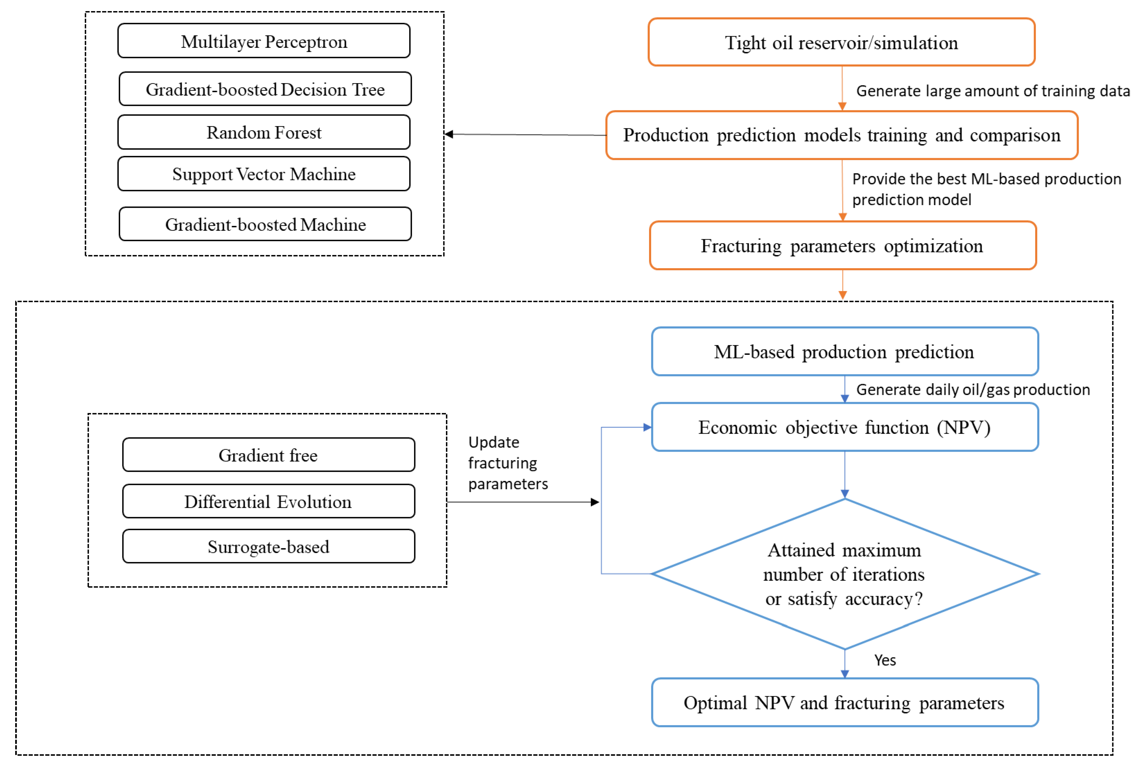
Figure 2.
Basic Configuration of a Neural Network.
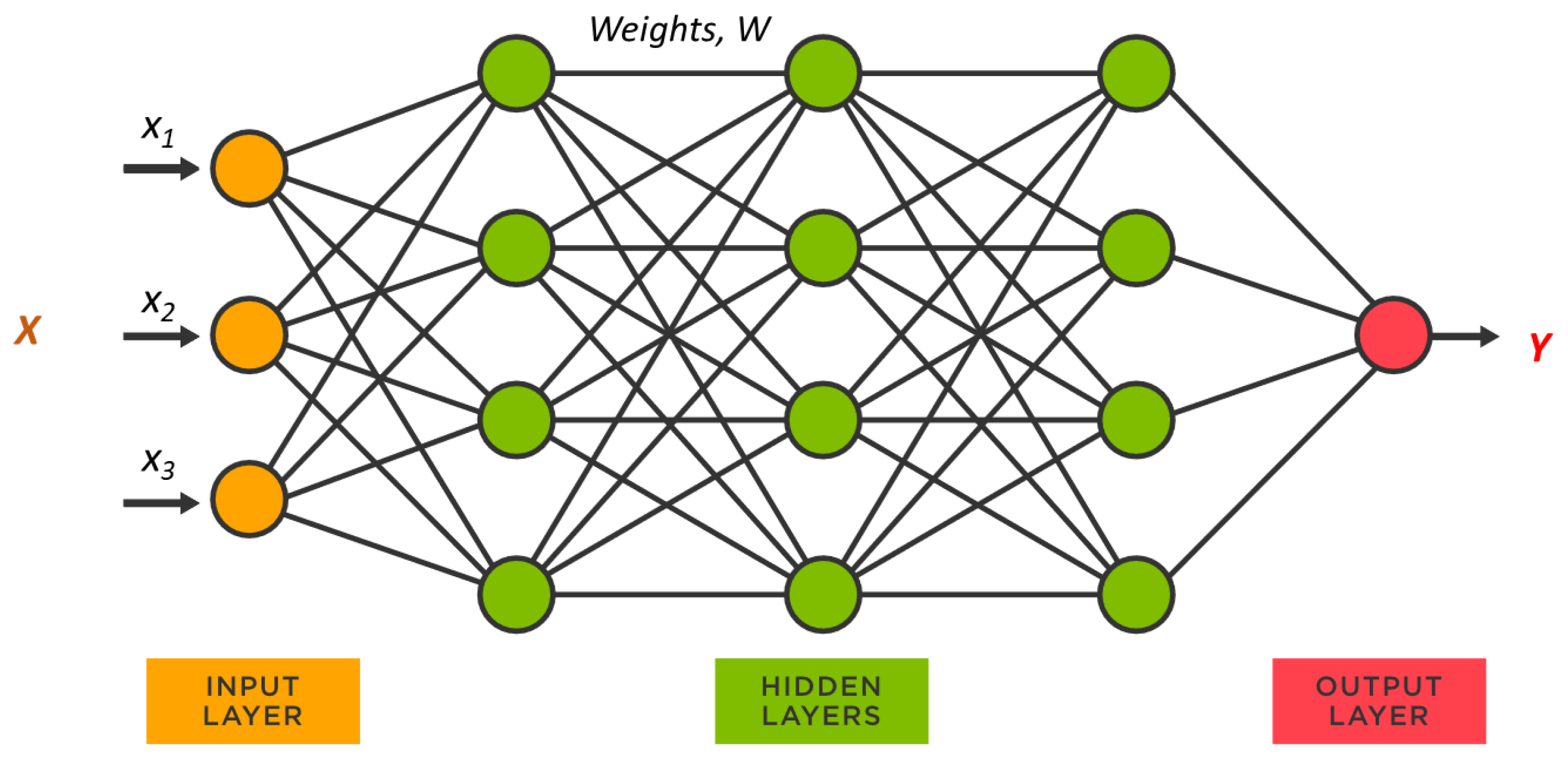
Figure 3.
Basic principles of RF [Adapted from (Dong et al., 2022)]
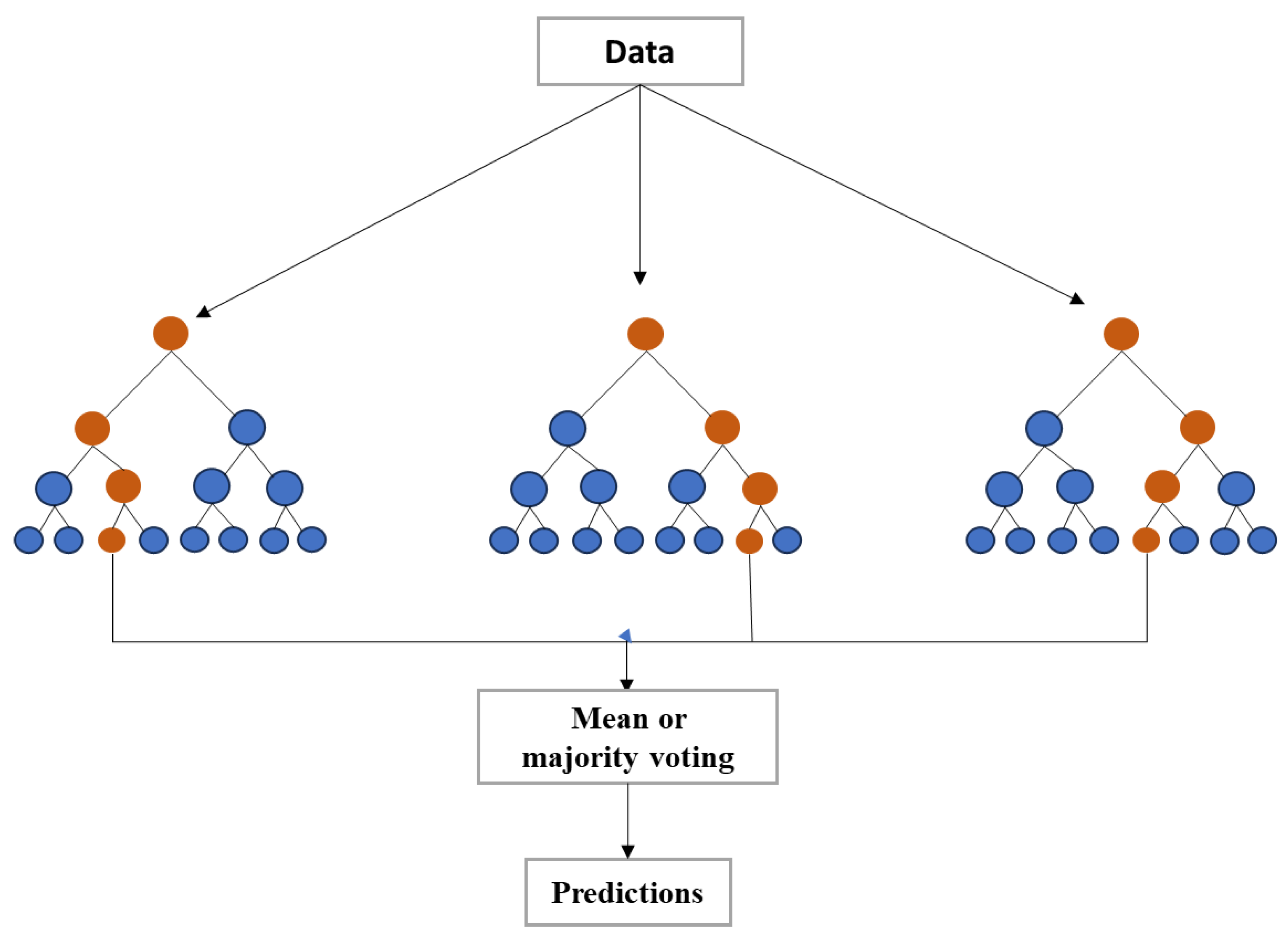
Figure 4.
Overfitting [Adapted from (Morozov et al., 2020)].
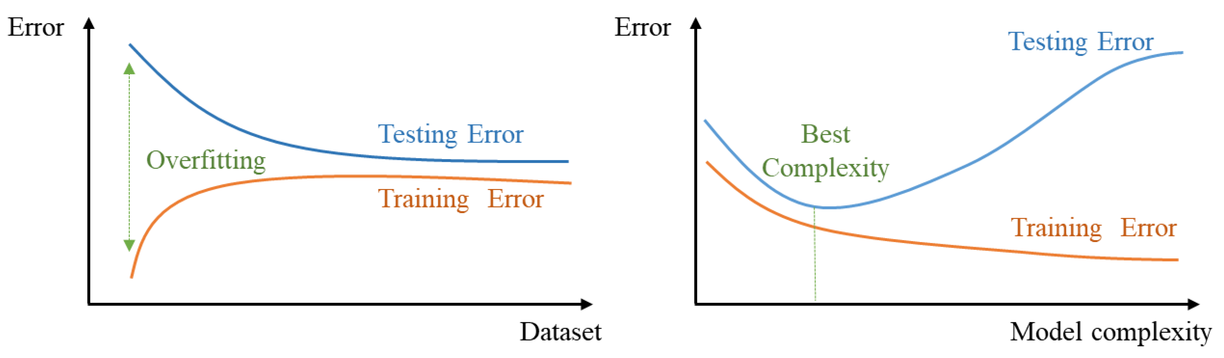
Figure 5.
(a) Feature ranking (b) Regression plot for the CatBoost Model [(Morozov et al., 2020)].
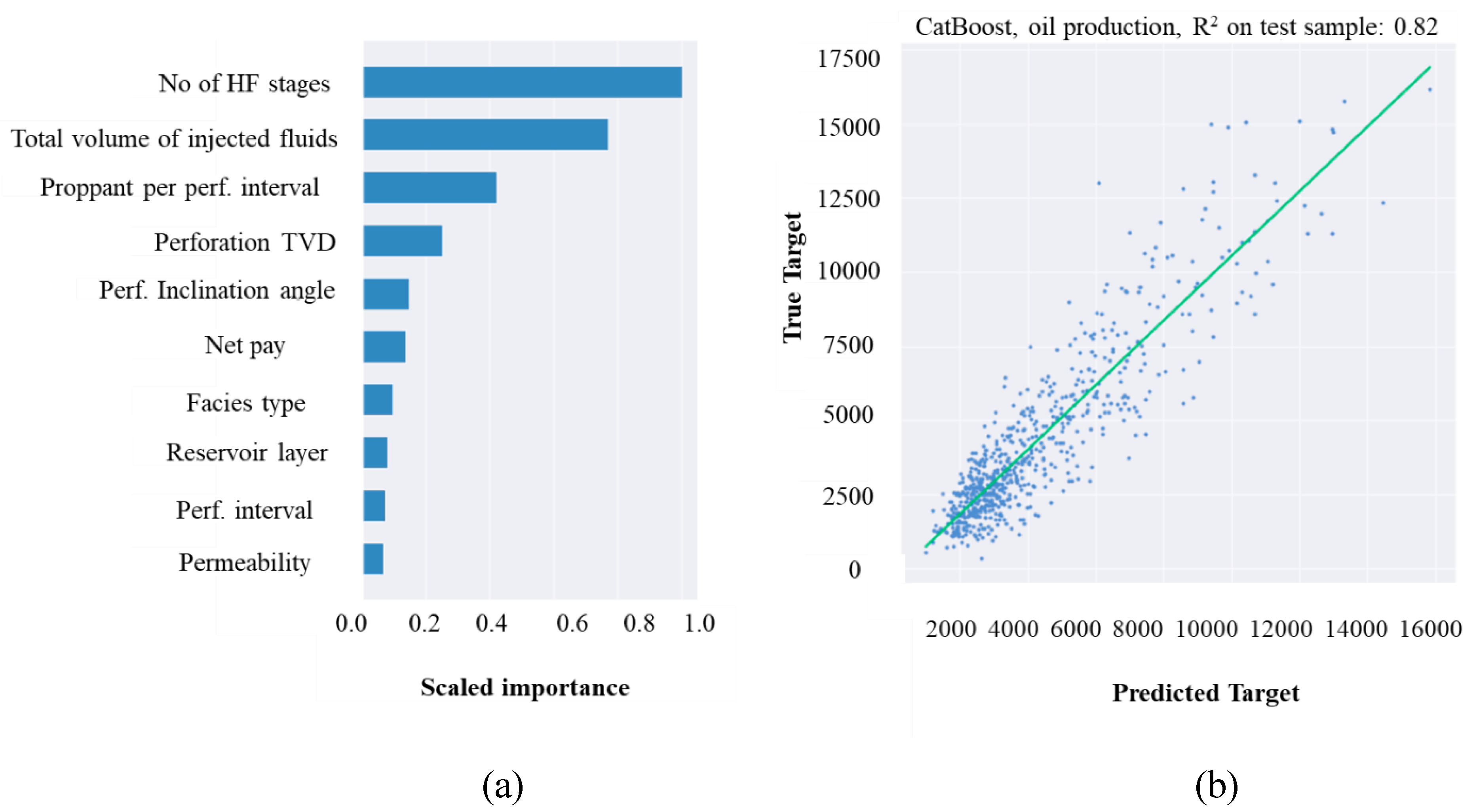
Figure 6.
Flowchart showing the process from geological modeling to reservoir simulation of shale (Lu, Jiang, Yang, et al., 2022).
Figure 6.
Flowchart showing the process from geological modeling to reservoir simulation of shale (Lu, Jiang, Yang, et al., 2022).
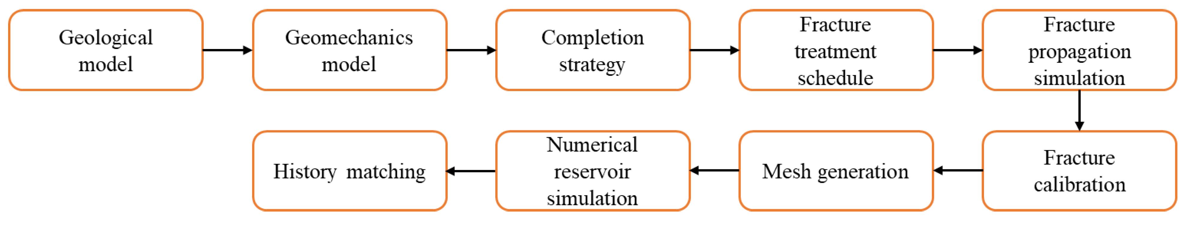
Figure 7.
Predicted EUR value vs. Estimated values using RF: (Ibrahim, Alarifi and Elkatatny, 2022). Without including Qi as an input feature; With Qi included as an input feature.
Figure 7.
Predicted EUR value vs. Estimated values using RF: (Ibrahim, Alarifi and Elkatatny, 2022). Without including Qi as an input feature; With Qi included as an input feature.
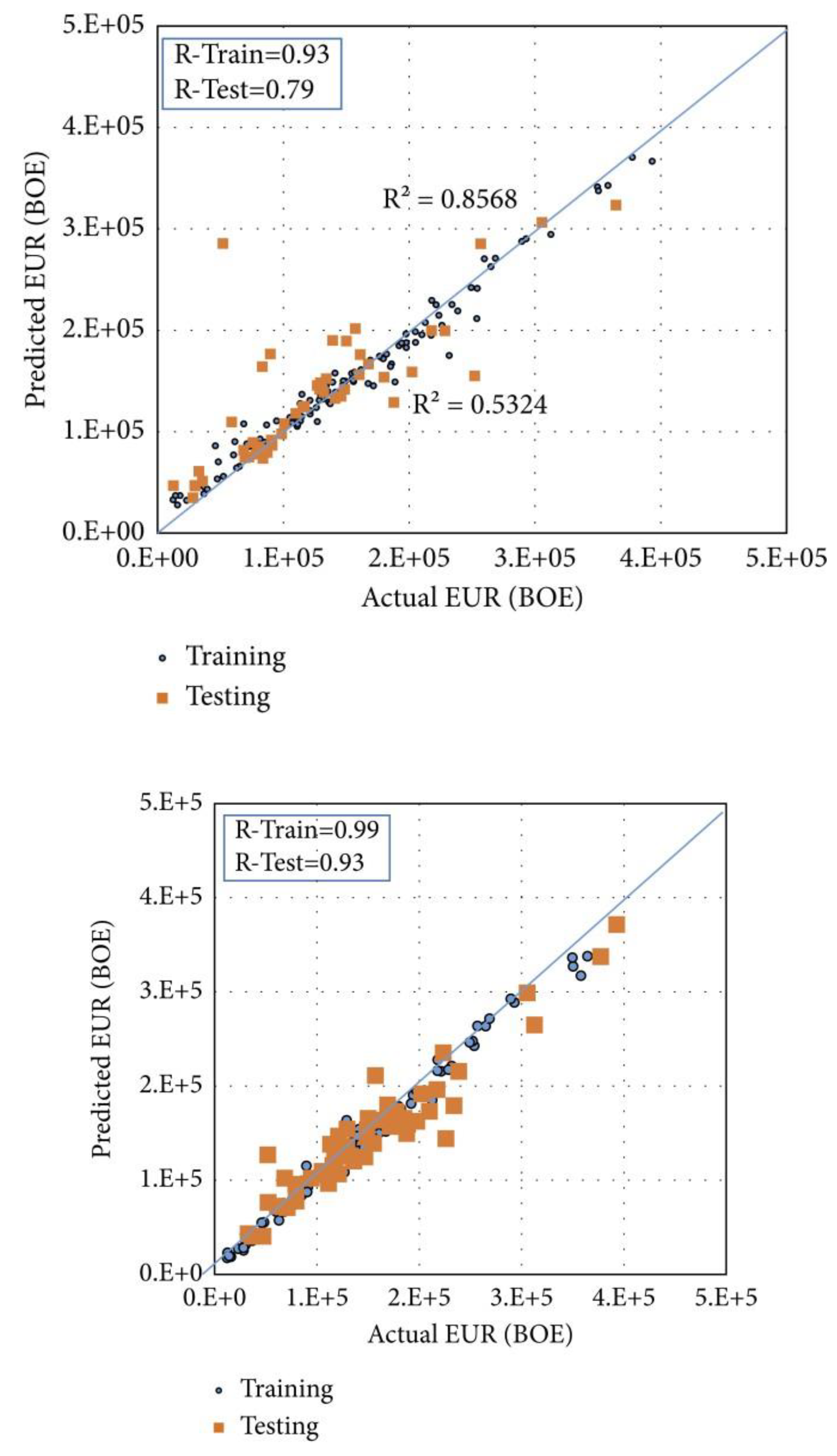
Figure 8.
Optimized cumulative production for different algorithms. (Duplyakov et al., 2022).
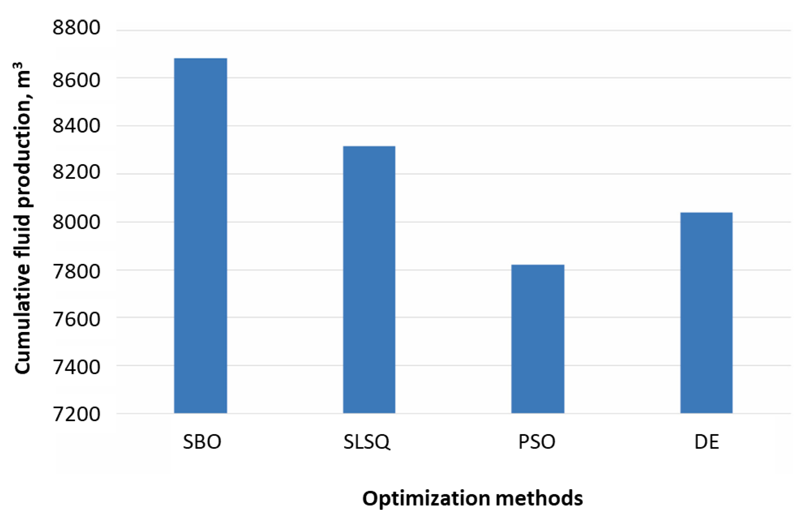
Figure 9.
Average recommended parameter (a – fluids rate, b - average proppant concentration, c – proppant mass per stage, d – final proppant concentration, e – pad share, f – epsilon) for the wells within optimal intervals (Duplyakov et al., 2022).
Figure 9.
Average recommended parameter (a – fluids rate, b - average proppant concentration, c – proppant mass per stage, d – final proppant concentration, e – pad share, f – epsilon) for the wells within optimal intervals (Duplyakov et al., 2022).
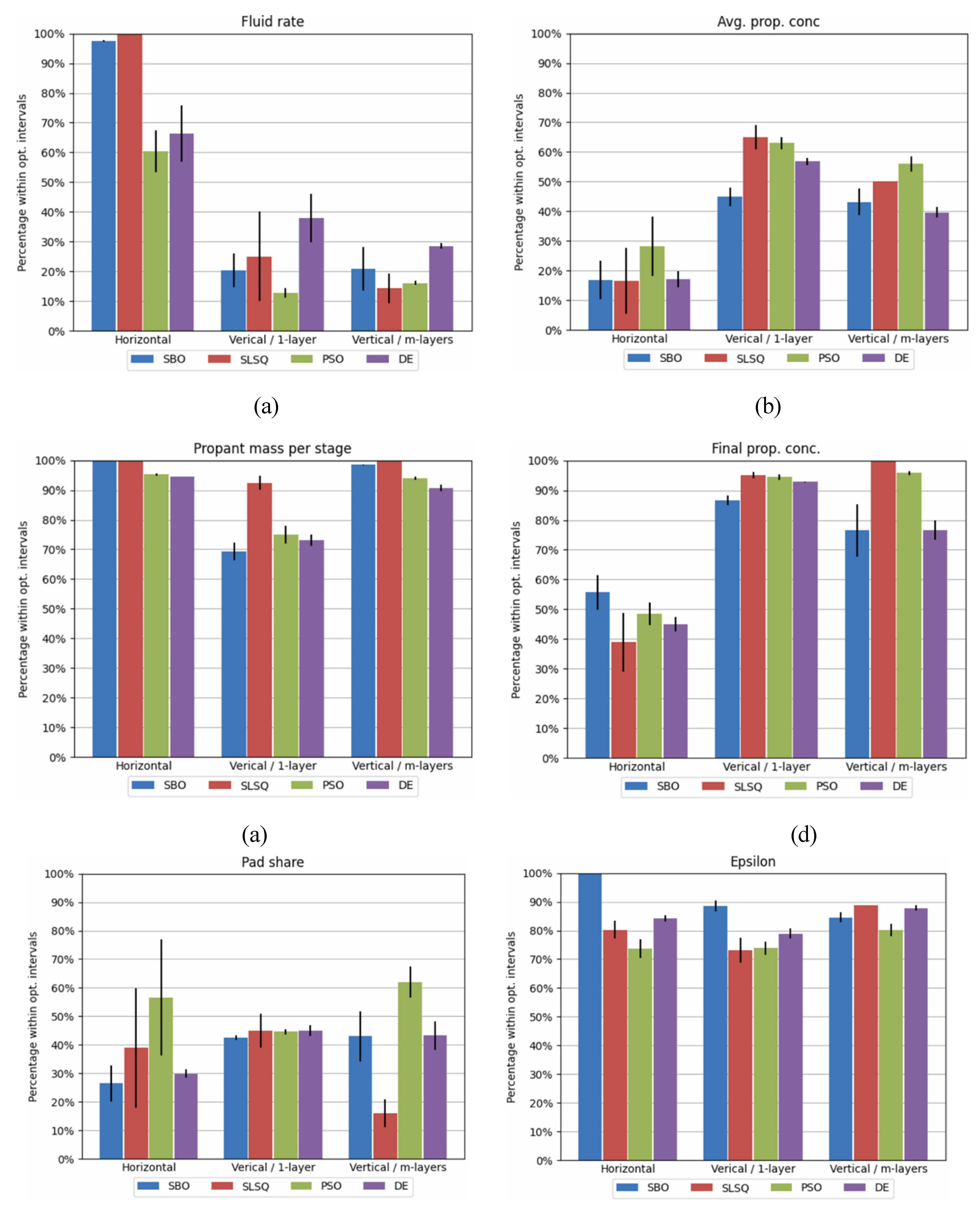
Figure 10.
NPV Sensitivity to fracturing parameters. (Dong et al., 2022).
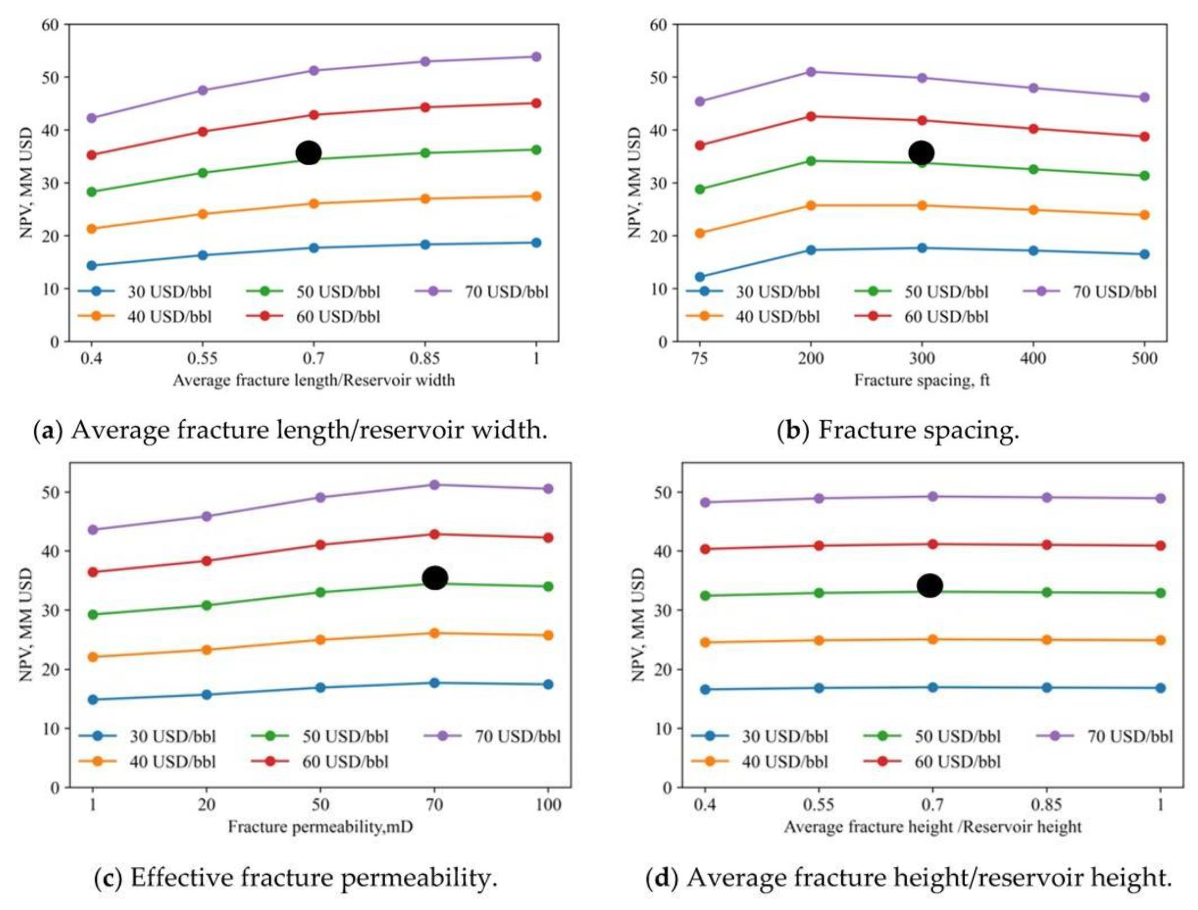
Figure 11.
NPV development across iterations for different optimization algorithms. (Dong et al., 2022).
Figure 11.
NPV development across iterations for different optimization algorithms. (Dong et al., 2022).
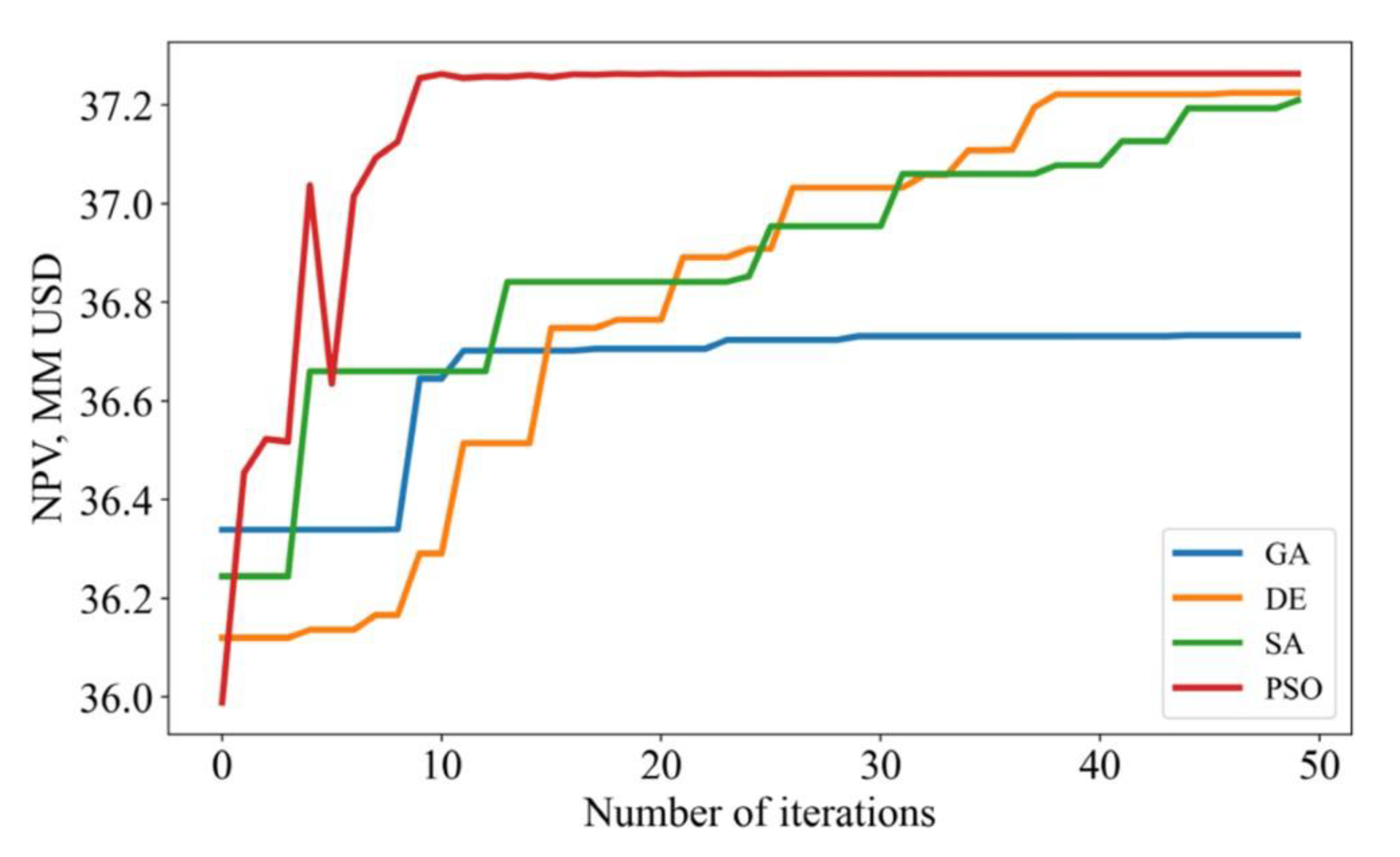
Figure 12.
(Lu, Jiang, Yang, et al., 2022); Normal NPV development; NPV evolution for the 4 extreme cases.
Figure 12.
(Lu, Jiang, Yang, et al., 2022); Normal NPV development; NPV evolution for the 4 extreme cases.
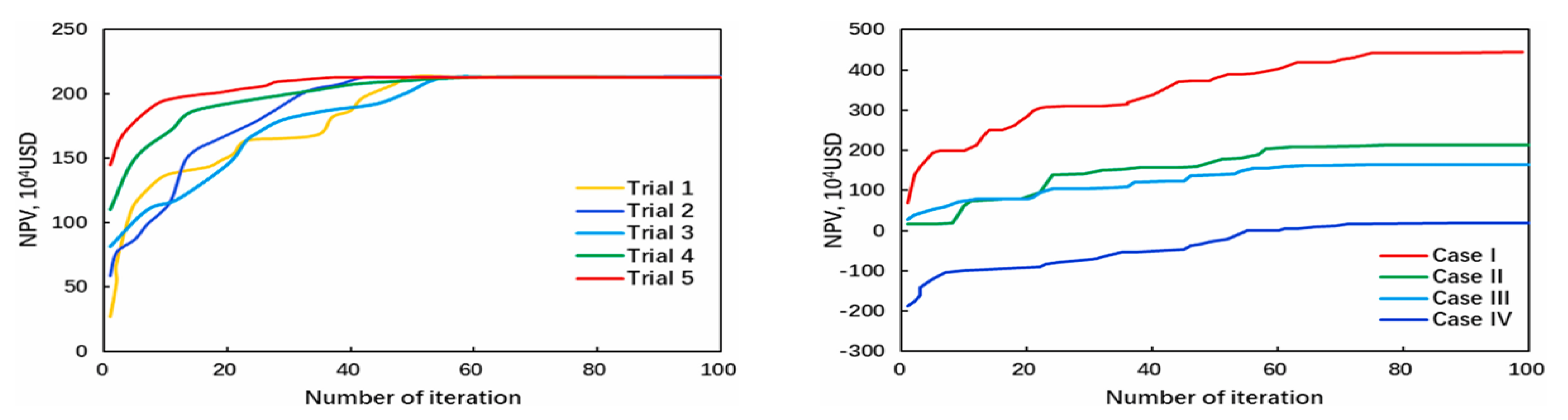
Figure 13.
Numerical simulation completion design for the 4 extreme cases. (Lu, Jiang, Yang, et al., 2022).
Figure 13.
Numerical simulation completion design for the 4 extreme cases. (Lu, Jiang, Yang, et al., 2022).
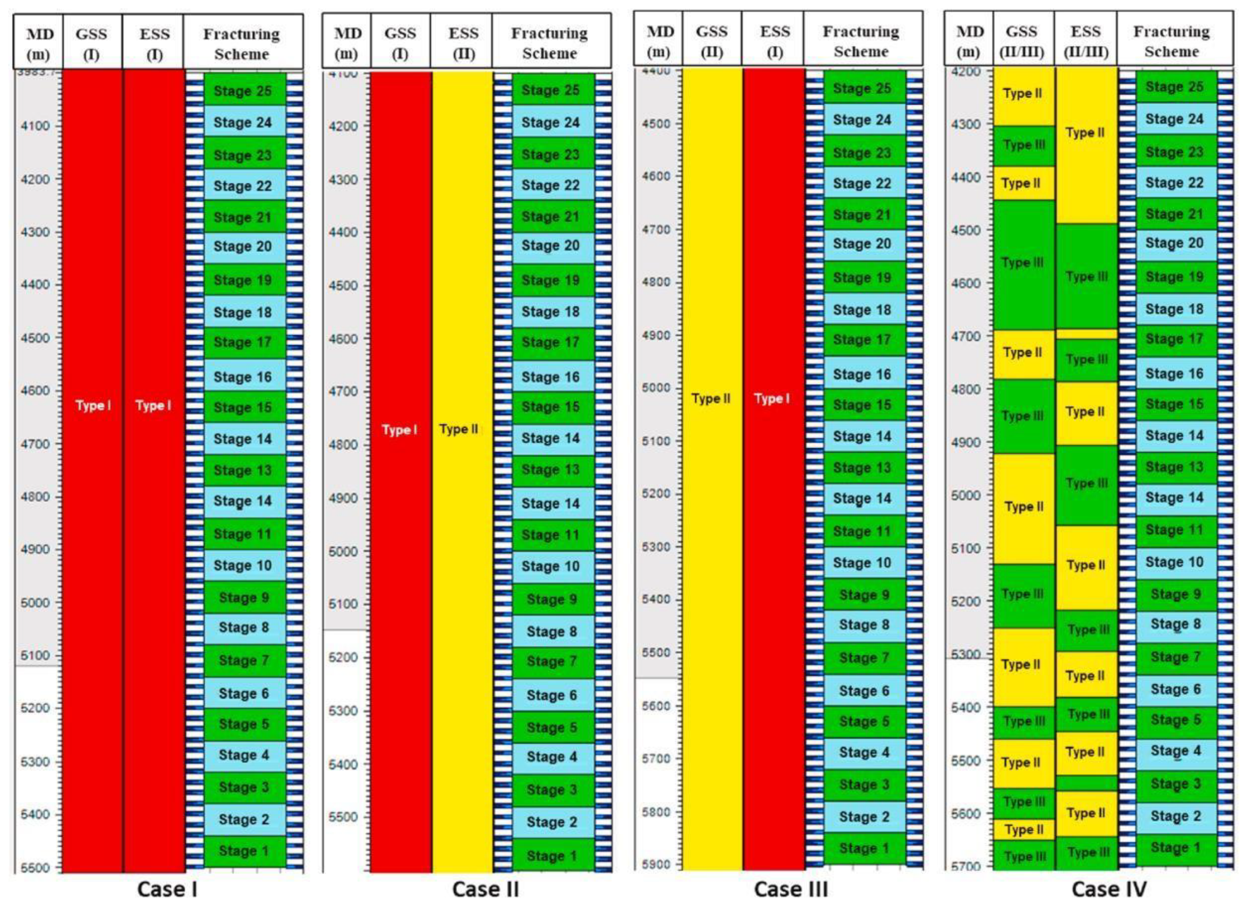
Figure 14.
NPV development for: (Xiao et al., 2022); (a) 500 training samples for all optimization algorithms; (b) Different training samples for MLP-DE compared with Eclipse.
Figure 14.
NPV development for: (Xiao et al., 2022); (a) 500 training samples for all optimization algorithms; (b) Different training samples for MLP-DE compared with Eclipse.
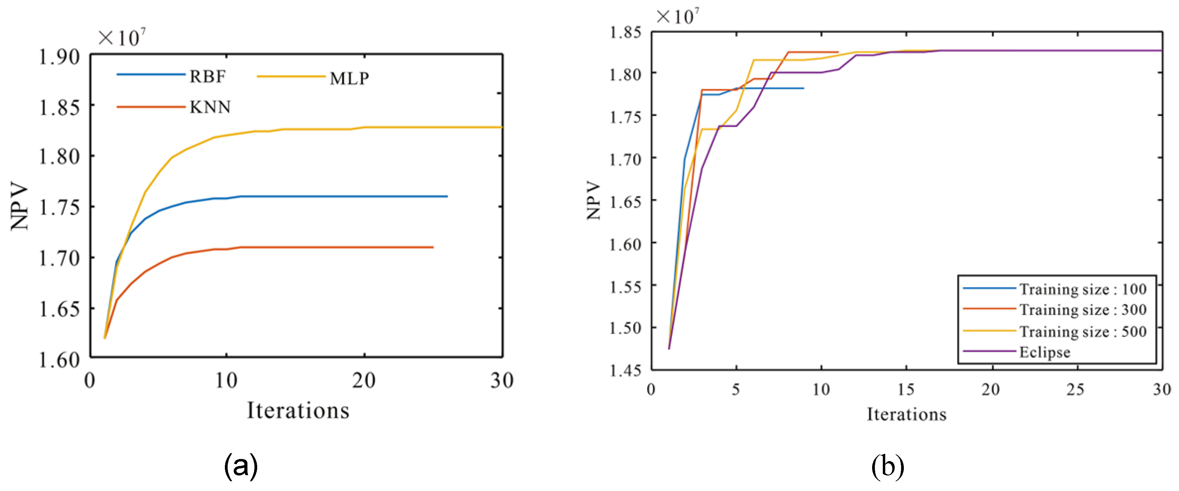

Table 1.
Parameters for the database building and their value ranges (Lu, Jiang, Yang, et al., 2022).
Table 1.
Parameters for the database building and their value ranges (Lu, Jiang, Yang, et al., 2022).
| Parameter | Unit | Range |
|---|---|---|
| Ratio of type 1, type II or type III GSS | - | 0 – 1 |
| Ratio of type I, type II, or type III ESS | - | 0 – 1 |
| Horizontal well length | m | 1000 – 3500 |
| Stage number | - | 9 – 45 |
| Cluster number per stage | - | 1 - 9 |
| Fluid volume | m3 | 10,000 – 70,000 |
| Proppant volume | m3 | 700 – 5,000 |
| Pump rate | m3/min | 4 – 15 |
Table 2.
Result summary of the DNN model (Lu, Jiang, Yang, et al., 2022).
| Production time | Data set | Evaluation matrices | ||
|---|---|---|---|---|
| Average MAE | Average MSE | Average R2 | ||
| 1 year | Training set | 0.26 | 0.14 | 0.90 |
| Validation set | 0.35 | 0.21 | 0.85 | |
| Testing set | 0.83 | 0.65 | 0.80 | |
| 5 years | Training set | 0.48 | 0.33 | 0.92 |
| Validation set | 0.63 | 0.41 | 0.87 | |
| Testing set | 0.74 | 0.45 | 0.84 |
Table 3.
Summary of results for DNN, RF, and SVM for 1-year post-production forecast. (Lu, Jiang, Yang, et al., 2022).
Table 3.
Summary of results for DNN, RF, and SVM for 1-year post-production forecast. (Lu, Jiang, Yang, et al., 2022).
| Evaluation model | Data set | Evaluation matrices | ||
|---|---|---|---|---|
| Average MAE | Average MSE | Average R2 | ||
| DNN | Training set | 0.48 | 0.33 | 0.90 |
| Validation set | 0.63 | 0.41 | 0.85 | |
| Testing set | 0.74 | 0.45 | 0.80 | |
| RF | Training set | 0.68 | 0.54 | 0.87 |
| Validation set | 0.94 | 0.82 | 0.83 | |
| Testing set | 1.17 | 1.95 | 0.75 | |
| SVM | Training set | 0.69 | 0.57 | 0.85 |
| Validation set | 0.87 | 0.81 | 0.80 | |
| Testing set | 1.68 | 2.31 | 0.72 |
Table 4.
Selected optimal hyperparameters. (Ibrahim, Alarifi and Elkatatny, 2022).
| Parameter | Optimum option | |
| Qi model | EUR model | |
| ANN model | ||
| No of hidden layers | Single hidden layer | Single hidden layer |
| Number of neurons in each layer | 8 | 8 |
| Training/testing split ratio | 70%/30% | 70%/30% |
| Training algorithms | Trainbr | Trainbr |
| Transfer function | Logsig | Logsig |
| Learning rate | 0.05 | 0.05 |
| RF | ||
| Maximum features | Sqrt | Auto |
| Maximum depth | 20 | 30 |
| Number of estimators | 150 | 100 |
Table 5.
Feature importance evaluation (Ibrahim, Alarifi and Elkatatny, 2022).
| Feature | Importance | Feature | Importance | Feature | Importance |
|---|---|---|---|---|---|
| FBR30 | 0.104806 | FBR60 | 0.096971 | FBR90 | 0.092448 |
| FBR180 | 0.096902 | CGP30 | 0.108577 | CGP60 | 0.100072 |
| CGP90 | 0.095441 | CGP180 | 0.093610 | CGP365 | 0.102260 |
| TP | 0.108912 |
Table 6.
Scheme 3 result (Ibrahim, Alarifi and Elkatatny, 2022).
| Data set/criterion | RF | KNN | SVM | GBDT |
|---|---|---|---|---|
| Training set, R2 | 0.7756 | 0.7983 | 0.8124 | 0.7865 |
| Test set, MAPE | 17.08% | 15.61% | 13.41% | 19.14% |
Table 7.
Selected Studies on production prediction of hydraulically fractured wells using ML.
| S/ N | Data Source | Input | Target | ML algorithm |
Hyperparameters | Split Train/ CV/ Test | Test R2 Or MAPE | Notes | Citation | |||||||||||||
|---|---|---|---|---|---|---|---|---|---|---|---|---|---|---|---|---|---|---|---|---|---|---|
| 1 | 20 oilfields (~6000 wells) in Western Siberia, Russia | 92 input variables, including reservoir geometry, fracturing parameters, and production data. | EUR | CatBoost | Depth = 7 L2 leaf reg = 0.6 LR = 0.02 Od type = ‘iter’ Od wait = 5 |
70/0/30 | 0.815 | OVAT analysis was performed to determine the ranking and correlation between features. Recursive feature elimination was used to reduce the initial 50 parameters to 35. |
(Morozov et al., 2020) |
|||||||||||||
| 2 | 841 numerical simulation data for training 97 field data oilfields in Jimusar sag and Xinjiang, China for Testing. |
Well data, Formation data, Completion data, Reservoir sweet spot mapping. |
EUR after 1 year EUR after 5 years |
DNN RF SVM |
LR = 0.003 Sigma = ReLu Hidden layers = 3 Neuron in each layer = 150 |
80/0/20 |
One year EUR 0.8 (DNN) 0.75 (RF) 0.72 (SVM) 5 years EUR 0.84 (DNN) |
The computational framework proposed by this study has better computational cost compared with traditional simulation. | (Lu, Jiang, Yang, et al., 2022) | |||||||||||||
| 3 | 200 well production data and completion | Stage count, Horizontal length, TVD, | Qi (BOE/mont h) | ANN RF |
See Table 4 | 70/0/30 |
RF 0.95 (Qi) 0.93 (EUR) |
Incorporating Qi as input for EUR estimation significantly | (Ibrahim, Alarifi and Elkatatny, 2022) | |||||||||||||
| design from Niobrara shale formation, North America. | Max treatment pressure, Total proppant volume, Total fluid volume |
EUR (BOE) |
ANN 0.96 (Qi) 0.99 (EUR) |
improved performance. For example, for RF, R2 was 0.79 without Qi vs. 0.93 with Qi. |
||||||||||||||||||
| 4 | 161 fractured wells data collected from Chang-Nig and Wei-Tuan blocks in China shale gas development zones | Geological and engineering parameters Flowback rate (FBR) Cumulative Gas Production (CGP) |
EUR (m3) | RF KNN SVM GBDT |
Not available (N/A) | 70/0/30 |
MAPE 17.08% (RF) 15.61% (KNN) 13.41% (SVM) 19.14% (GBDT) |
The gini index was used to find the 10 most important input factors. As a linear classifier, SMV performs best because of the linear relationship between early production data and EUR. | (Niu, Lu and Sun, 2022) | |||||||||||||
| 5 | 573 horizontal wells from Duvernay Formation of Fox Creek, Alberta | 13 geological (E.g., Duvernay thickness, porosity, gas saturation) and operational (total injection, total proppant, stage number, well TVD) factors. | 12-month shale gas production | Linear regression (LR) Neural Network (NN) GBDT Extra Trees (ET) |
N/A | 80/0/20 | 0.729 (NN) 0.809 (ET) 0.794 (GBDT) 0.653 (LR) |
ET gives the best prediction with just 9 features, which is the lowest number of features of all algorithms studied. | (Hui et al., 2021) | |||||||||||||
| 6 | 2000 samples were generated via numerical simulation. |
Geological (formation thickness, matrix permeability, initial pressure, matrix porosity) and engineering (SRV porosity, SRV permeability, HFs conductivity, HFs half-length, stage number of HFs) factors |
Shale gas production | Multi- objective random forest (MORF) Multi- objective regression chain (MORC) |
MORF (without initial production) No of trees = 190 No of features = 9 Max depth = 18 MORF (with initial production) No of trees = 190 No of features = 10 Max depth = 18 MORC (with initial production) No of trees = 110 No of features = 10 Max depth = 13 |
70/0/30 | 0.9229 (MORF w/o initial prod)) 0.9467 (MORF with initial prod) 0.9356 (MORC with initial prod) |
Given initial production data, MORF is superior to MORC because, at the intermediate production stage, the transition from highly declining to stable production is non- linear. This indicates that MORC may be less suited for dealing with non- linear changes. | (Xue et al., 2021) | |||||||||||||
| 7 | 815 viable simulation cases. Numerical model built from geological and fluid parameters from Bakken Shale Oil, North America. |
Thickness, matrix permeability, natural fracture permeability, BHP, horizontal well length, number of hydraulic fractures, stage spacing, fracture half-length, fracture aperture, | Daily production (DP) for 10 years. Cumulative production (CP) for the first 10 years |
Deep belief network (DBN) Back propagation NN Support vector regression (SVR) |
DBN Sigma = ReLu Group out = 0 Hidden layers = 2 Hidden neurons = 155 (for DP); 185 (for CP) DBN LR = 0.02 RBM LR = 0.02 (for DP); 0.08 (for CP) Iteration = 260 (for DP); 350 (for CP) Batch size = 7 |
80/0/20 |
DBN 0.9062 (DP) 0.9379 (CP) BP 0.8287 (DP) 0.9049 (CP) SVR 0.8490 (DP) 0.8561 (CP) |
DBN is superior to BP and SVR. When the hyperparameters are well-tuned, DBN is great for scenarios where the production trend is anomalous to a typical shale well. | (Wang et al., 2021) | |||||||||||||
| fracture conductivity, fracturing fluid injection, Soaking time | Epoch of RBM = 16 (for DP); 28 (for CP) | |||||||||||||||||||||
| 8 | 2919 wells, including 2780 multi-stage hydraulic fractured horizontal wells and 139 vertical wells in the Bakken Formation |
18 parameters consisting of well, formation fractures, fracturing fluid, and proppant data. | 6-month oil production 18-month oil production |
DNN | Dropout layer = no Activation function = ReLu Network model config = uniform model LR = 0.005 Layer no = 3 Neurons for each hidden layer = 200 |
81/9/10 | 0.71 (6- month) 0.72 (18- month) |
Given the wide discrepancy between train and test R2 (0.87 vs. 0.71 and 0.94 vs. 0.72) for 6- and 18-month post- production prediction, it suggests the model might be overfitted. |
(Wang and Chen, 2019) | |||||||||||||
| 9 | 989 multistage hydraulically fractured horizontal wells from four formations - Niobrara, Barnett, Eagle Ford, and Bakken | Completion parameters Normalised completion parameters Production parameters ( 3 months and 2 years of production data) |
EUR | ANN | N/A | 70/0/30 | The result is formatted as: Formation (2 years R2 / 3 months R2) Niobrara (0.996/0.904) Barnett (0.972/0.769) Eagle Ford |
With just 3 months of production data, EUR estimation has an R2 between 0.72 and 0.9 for all formations. This increases to > 0.97 after 2 years data is available. Since decline curve analysis (DCA) only provides an |
(Alarifi and Miskimins, 2021) | |||||||||||||
| (0.978/0.819) Bakken (0.984/0.716) |
accurate estimate after 3 years of production data, ANN can better estimate EUR in the early life of a production well. | |||||||||||||||||||||
| 10 | 129 horizontal wells in the gas Eagle Ford Shale. | 18 geological and fracturing parameters. Some include proppant volume, tubing head pressure, gas gravity, measured depth, TVD, gas oil ratio, etc |
Cumulative gas production (36 months) | RF Gradient Boosting Machine (GBM) SVM |
RF Mtry = 5 Ntree = 300 GBM Mtry = 5 Ntree = 20 SVM Penalty function = 600 Kernel parameter (RBF) = 20 |
80/0/20 | 0.69 - RF (VIM %IncMSE) 0.73 - RF (VIM IncNodePurity) 0.69 - GBM (VIM IncNodePurity) 0.63 - SVM (Kernel function) |
After clustering analysis on the dataset, there was an improvement in prediction. RF R2 was 0.4 for all datasets, and after clustering, that increased to 0.74 for cluster 1 and 0.88 for cluster 2. |
(Han, Jung and Kwon, 2020) | |||||||||||||
Table 8.
Parameters and the distribution for the input data set (Dong et al., 2022).
| Parameter | Minimum value | Maximum value | Distribution type | Symbol |
|---|---|---|---|---|
| X grid, ft | 75 | 125 | Uniform | DI |
| Y grid, ft | 30 | 80 | Uniform | DJ |
| Z grid, ft | 1 | 5 | Uniform | DK |
| Matrix permeability, mD | 0.0001 | 1 | lognormal | PERM |
| Porosity | 0.05 | 0.15 | Uniform | POR |
| Horizontal well length, ft | 1800 | 6000 | Triangle | WellLength |
| Bubble-point pressure, psi | 400 | 6000 | Uniform | PB |
| Initial pressure, psi | 2000 | 6000 | Uniform | INIT_PRES |
| Monitored oil rate, bbl/day | 1.5 | 2.5 | Triangle | MONITOR_STO |
| Operating BHP, psi | 200 | 3000 | Uniform | OPERATE_BHP |
| Average fracture length/ reservoir width | 0.4 | 1 | Uniform | FL/W |
| Fracture spacing, ft | 75 | 500 | Uniform | FS |
| Effective fracture permeability, mD | 1 | 100 | Uniform | FS |
| Average fracture height/ reservoir height | 0.4 | 1 | normal | FH/H |
Table 9.
Optimal hyperparameters for the evolutionary models examined.(Dong et al., 2022).
| Evolutionary Algorithm | Hyperparameters |
|---|---|
| GA | size_pop = 26; max_iter = 50; prob_mut = 0.001 |
| DE | size_pop = 26; max_iter = 50 |
| SA | max_stay_counter = 150 |
| PSO | size_pop = 26; max_iter = 50; w = 0.8, c1 = 0.5, c2 = 0.5 |
Table 10.
Optimization results of different optimization algorithms (Dong et al., 2022).
| Hybrid Model | MLP-GA | MLP-DE | MLP-SA | MLP-PSO |
|---|---|---|---|---|
| Fracture length/reservoir width | 0.98 | 0.98 | 0.97 | 0.99 |
| Fracture spacing, ft | 290 | 296 | 281 | 275 |
| Fracture permeability, mD | 88 | 75 | 94 | 89 |
| Fracture height/ reservoir height | 0.87 | 0.78 | 0.89 | 0.94 |
| No of iterations to stability | 11 | 38 | 48 | 9 |
| Maximum NPV, millions USD | 36.73 | 37.22 | 37.20 | 37.26 |
Table 11.
Parameters comparison between initial and optimal values (Lu, Jiang, Yang, et al., 2022).
| Parameter | Initial value | Optimal value |
|---|---|---|
| Horizontal well length, m | 147 | - |
| Ratio of GSS | 0.42, 0.22, 0.36 | - |
| Ratio of ESS | 0.34, 0.53, 0.13 | - |
| Number of stages | 26 | 28 |
| Number of clusters | 88 | 112 |
| Fluid volume, m3 | 47,376 | 55,388 |
| Proppant volume, m3 | 2422 | 2978 |
| Cumulative oil production, m3 | 29,694 | 32,663 |
| NPV, 104 USD | 145 | 213 |
Table 12.
Optimized fracture parameters determined by ML models and Eclipse simulator (Xiao et al., 2022).
Table 12.
Optimized fracture parameters determined by ML models and Eclipse simulator (Xiao et al., 2022).
| Model | Training size | NPV, yuan, 107 |
Simulation number | Fracture conductivity D-cm | Fracture halflength | Fracture spacing, m | Fracture number |
|---|---|---|---|---|---|---|---|
| Eclipse | - | 1.832 | 1500 | 42.28 | 46.8 | 17.9 | 46 |
| RBF | 500 | 1.761 | 500 | 38.42 | 41.2 | 19.6 | 42 |
| KNN | 500 | 1.710 | 500 | 45.24 | 42.3 | 18.7 | 44 |
| MLP | 100 | 1.762 | 100 | 31.41 | 41.5 | 19.2 | 43 |
| 300 | 1.821 | 300 | 40.25 | 46.1 | 17.9 | 46 | |
| 500 | 1.829 | 500 | 41.32 | 46.5 | 17.9 | 46 |
Disclaimer/Publisher’s Note: The statements, opinions and data contained in all publications are solely those of the individual author(s) and contributor(s) and not of MDPI and/or the editor(s). MDPI and/or the editor(s) disclaim responsibility for any injury to people or property resulting from any ideas, methods, instructions or products referred to in the content. |
© 2024 by the authors. Licensee MDPI, Basel, Switzerland. This article is an open access article distributed under the terms and conditions of the Creative Commons Attribution (CC BY) license (http://creativecommons.org/licenses/by/4.0/).
Copyright: This open access article is published under a Creative Commons CC BY 4.0 license, which permit the free download, distribution, and reuse, provided that the author and preprint are cited in any reuse.


