
Submitted:
31 January 2026
Posted:
04 February 2026
You are already at the latest version
Abstract
We present a four-dimensional, PT-symmetric quaternion-inspired extension of General Relativity formulated in a PT-even Palatini posture. Rather than treating a quaternionic "imaginary metric" as a physical spacetime tensor, we define the physical sector by a PT-even projection operator $\Pi_{PT}$ acting on the action and on composite observables:$$S_{phys} \equiv \Pi_{PT} [S(g, \Gamma, \phi; \epsilon)]$$ so that the measure and all reported observables are real by construction. The fundamental fields are a real (or PT-even) metric $g_{\mu\nu}$, an independent affine connection $\Gamma^{\lambda}_{\mu\nu}$ (allowing torsion), and a single real scalar spurion $\phi$ that controls a dimensionless flux amplitude $\epsilon \equiv 2\phi/M_{pl}$ in the connection/torsion sector. Nontrivial quaternionic/noncommutative effects are parameterized by a white-box operator basis $\Delta\mathcal{L} = \sum_i c_i \mathcal{O}_i(T_{\mu}, S_{\mu}, q_{\lambda\mu\nu}, g; \epsilon)$, built from the irreducible torsion components, with PT selection rules specifying which operators survive in $S_{phys}$.We then adopt a minimal-alignment phenomenology: the same spurion family $\epsilon$ is represented by scale-dependent templates $\epsilon(t)$, $\epsilon(r)$, and $\epsilon(E_T)$, which can be confronted with public data across three regimes:(i) late-time acceleration in SN Ia cosmology;(ii) approximately flat galaxy rotation curves in the SPARC sample;and (iii) missing transverse energy spectra at the LHC.In this work, we emphasize interpretational consistency: the three profiles are not claimed to arise from one universal PDE valid across all scales; instead, they are effective templates corresponding to different kinematic reductions of the same PT-even spurion sector, with scale-dependent effective couplings. The Palatini torsion posture provides an immediate diagnostic interface to stability. Crucially, consistent with the companion symmetry analysis, the PT-even projection imposes a coefficient-locking identity (C3) that enforces equality between the gravitational and kinematic couplings ($K=G$) for tensor modes. This structural locking guarantees exact tensor luminality ($c_T = 1$) at the leading order without parameter tuning, naturally satisfying the stringent GW170817 constraints. This work therefore serves as the phenomenological front-end, applying the strictly bounded PT-even framework to public data.
Keywords:
PT symmetry
; quaternion-inspired geometry
; Palatini gravity
; torsion decomposition
; PT-even projection
; operator basis
; dark energy
; galaxy rotation curves
; missing transverse energy
; noncommutative geometry
; GW170817
; DESI
; HL–LHC
; LISA
1. Introduction and Physical Motivation
General Relativity (GR) and Quantum Mechanics (QM) anchor modern physics. GR describes gravity through spacetime geometry [4], whereas QM encodes microscopic phenomena in complex probability amplitudes [5]. Despite remarkable empirical success, their conceptual interface remains unsettled: GR is built on a dynamical classical manifold, while QM is typically formulated on a fixed background with Hermitian operators. In cosmology and astrophysics this gap is packaged into the CDM paradigm [26], whose phenomenological components—dark energy and dark matter—dominate the cosmic energy budget but lack a universally accepted microphysical origin. At the same time, multi-messenger observations (most notably GW170817) and precision tests increasingly constrain infrared modifications of gravity, motivating frameworks that are explicit about what is physical, what is projected out, and how the stringent tensor luminality is guaranteed.
Guiding constraint (Symmetry-Guaranteed Framework).
Any geometric extension that aims to “explain the dark sector” must be engineered with a clear diagnostic interface. It is no longer sufficient to merely fit data; the theory must structurally explain why gravitational waves propagate at the speed of light () without fine-tuning. In this work, we elevate the discussion from a phenomenological model to a symmetry-guaranteed framework. We adopt the viewpoint that PT symmetry and quaternion-inspired structures serve as organizing principles, implementing a coefficient-locking mechanism that renders the theory safe under standard gravitational diagnostics. A rigorous foundation for such a PT-even Palatini framework, guaranteeing tensor luminality from symmetry, was recently established in Ref. [1].
1.1. PT-Even Projection Principle and What Is Physical
Quaternionic or noncommutative constructions often suggest geometric objects with explicitly non-real components. Interpreting an “imaginary metric” as a physical spacetime tensor, however, immediately raises two technical issues: (i) defining a real measure (determinant/volume form) is nontrivial in quaternionic settings, and (ii) the status of covariant derivatives and curvature becomes ambiguous when mixing commutative differential geometry with noncommutative algebraic operations. To avoid these pitfalls while preserving the intended PT-symmetric content, we adopt a minimal but strict principle:
Physical observables and the physical action are defined by projecting to the PT-even sector.
Concretely, we introduce a PT-even projection operator and define
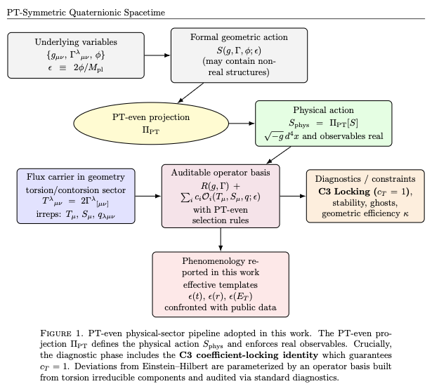
so that the measure and all reported observables are real by construction. In this work we take to be real (or identified with the PT-even part of a more general object) and use the standard volume form in . Figure 1 summarizes the “physical-sector” pipeline adopted throughout.
1.2. Geometry Choice: Palatini Posture with Torsion as the Flux Carrier
To keep the geometry self-consistent and compatible with standard diagnostics, we work in a Palatini posture in which the metric and connection are independent variables. The fundamental fields are
where is a real scalar spurion that controls a dimensionless flux amplitude . Quaternionic/noncommutative effects are not encoded as a physical imaginary metric component, but as a PT-even spurionic structure in the connection/torsion sector. We define torsion as usual by
and employ its standard irreducible decomposition into a trace vector , an axial vector , and a traceless tensor . This choice is aligned with the companion-series operator diagnostics (trace/axial/traceless selection rules) and provides a bridge between quaternion-inspired “flux” intuition and conventional gravitational EFT language.
1.3. From Black-Box Curvature Corrections to a Symmetry-Guaranteed Basis
A recurring weakness of early phenomenological models is the use of a black-box term—schematically —that absorbs all nonstandard effects without specifying which operators are present and which are absent. Such a black box makes it impossible to audit stability or tensor-sector constraints. Here we instead parameterize the deviation from Einstein–Hilbert by a finite operator basis built from the torsion irreps:
where the subscript indicates PT-even projection through . Most importantly, the coefficients are not arbitrary. As we shall see in Section 2.5, symmetry imposes a coefficient-locking identity (C3) that enforces equality between the kinetic and gradient terms of the tensor perturbations (). This structural guarantee ensures that the theory remains luminal () at the leading order.
1.4. Minimal-alignment Phenomenology Across Three Regimes
With the PT-even Palatini/torsion framework fixed, we introduce a single spurion family whose observable imprint is represented by three scale-dependent templates: for FLRW cosmology, for galactic dynamics (modulated by a geometric efficiency factor ), and for collider kinematics. A crucial interpretational point is that these profiles are not claimed to arise from one universal field equation valid across all length/energy scales. Rather, they should be viewed as effective templates corresponding to different kinematic reductions and different effective couplings of the same PT-even spurion sector. Figure 2 summarizes this three-regime minimal-alignment viewpoint.
We confront the templates with three public-data arenas: SN Ia cosmology (Section 3.1), SPARC galaxy rotation curves (Section 3.2), and CMS missing transverse energy spectra (Section 5.5). The purpose is to demonstrate that a unified PT-even spurion sector can reproduce the shapes typically attributed to dark energy, dark matter, and high-energy missing-energy tails, while remaining compatible with the diagnostic posture of the companion series.
1.5. Structure of the Paper
The paper is organized as follows. Section 2.6 formulates the PT-even projection principle and the crucial Luminality Guarantee (Locking Identity). Section 3.1 applies the spurion template to FLRW cosmology and discusses its interpretation as an effective geometric source. Section 3.2 constructs the galactic template via the geometric efficiency factor and tests it against the SPARC rotation curves. Section 5.5 presents the high-energy template and its comparison to public CMS MET data. We conclude by summarizing falsifiable predictions and by linking the framework to its potential UV origin in D-Branes.
2. Theoretical Framework
This section provides the theoretical backbone used throughout this work. Moving beyond a purely phenomenological construction, we adopt a symmetry-guaranteed framework formulated in a PT-even Palatini posture. The guiding choice is to keep the metric sector real and to encode the quaternion-inspired “flux” as a PT-even spurionic structure carried by the independent connection (torsion/contorsion). The goal is not to present a fully derived quaternionic noncommutative geometry (which would require a careful treatment of measures and curvature in ), but rather to define an auditable and diagnostic-compatible effective framework that can support the three phenomenological templates used later: (cosmology), (galaxies), and (colliders).
For motivation only, one may heuristically write quaternionic-inspired coordinates
but in the present strategy these extra components are not treated as physical coordinates nor as an “imaginary metric” sector. Instead, their intended effect is captured by a single real spurion (or equivalently ) entering the PT-even torsion/connection sector.
2.1. PT-even Projection Principle and the Physical Sector
A key vulnerability of early quaternionic constructions is the lack of a defensible definition of (i) a real measure/volume element and (ii) a unique curvature/variation principle once noncommutativity is introduced. The remedy adopted here is to impose a strict physical-sector selection rule:
Physical observables and the physical action are defined by projecting to the PT-even sector.
We implement this using a PT-even projection operator . For any (possibly complex/quaternionic) quantity X, define
so that is PT-even by construction. In particular, the physical action is defined as
Variation–projection interchange (defensible posture).
To keep a standard variational principle, we adopt the following (series-aligned) assumption:
i.e. the projection commutes with the functional variation on the class of configurations considered. In a fully developed treatment this can be proven under mild regularity/boundary conditions (as in companion-series arguments); for the present work it is stated as the minimal consistency condition required to define a physical PT-even sector.
PT assignments (minimal).
We assume the spurion (and hence ) is PT-even, and we restrict attention to PT-even scalar operators in the effective action. PT-odd operators (including purely parity-odd invariants) are projected out by and do not contribute to .
2.2. Geometry Choice: Palatini Posture and Torsion Decomposition
We work in a Palatini posture in which the metric and connection are independent variables:
with units and . Matter fields are taken to couple minimally to (Jordan frame),
which enforces a “no-fifth-force baseline” in this framework.
Torsion as the flux carrier.
Quaternionic/noncommutative effects are encoded not as a physical imaginary metric component, but as PT-even spurionic structure in the connection, i.e. in torsion/contorsion. The torsion tensor is defined by
For readability and diagnostic control, we further adopt metric compatibility,
so that the departure from Levi–Civita geometry is carried by contorsion (rather than by nonmetricity). One may then write
where is the Levi–Civita connection of , and is the contorsion tensor related algebraically to torsion.
Irreducible decomposition (trace / axial / traceless).
It is convenient to decompose torsion into irreducible components: a trace vector , an axial (pseudo-)vector , and a traceless tensor . Define
and a traceless piece satisfying and . Then one may write (schematically)
This decomposition is the natural language for an auditable operator basis and for series-aligned selection rules.
Spurion amplitude.
We introduce a real scalar spurion and the dimensionless flux amplitude
In the minimal-alignment strategy is the universal bookkeeping parameter that controls the size of PT-even torsion-sector operators, while its functional form becomes regime-dependent in phenomenological reductions (, , ).
2.3. Measure and Determinant: Replacing the “Hard Cut”
A central defect of early quaternionic drafts was the ad hoc replacement , which is vulnerable because it does not define a quaternionic measure and is not derived from a symmetry principle. In the present framework, the measure is instead fixed by the PT-even physical-sector definition:
In practice, we implement this by choosing the physical metric to be real and using the standard volume form
This is the minimal defensible choice: it ensures real weights in the path integral and a standard variational principle, while all nontrivial “flux” information is carried by the PT-even torsion/connection operators.
2.4. Operator Basis and Diagnostics (White-Box Replacement of )
Another major vulnerability of early drafts was the use of a black-box term that “absorbs all nonstandard effects”. Such a term cannot be audited: it obscures which operators propagate extra modes, whether ghosts/gradients appear, and whether the tensor sector remains luminal. The remedy is to replace the black box by a finite PT-even operator basis built from torsion irreps.
Power counting and minimality.
We restrict to local operators that are: (i) PT-even scalars, (ii) at most quadratic in torsion irreps (for minimal EFT control), and (iii) do not introduce higher-derivative kinetic terms for the spin-2 sector at baseline. Under these restrictions, torsion is typically non-propagating (algebraic) at leading order and can be integrated out in principle.
A minimal PT-even torsion basis.
A representative PT-even basis (sufficient for the phenomenological narrative) is
together with PT-even spurion dressings such as . Boundary terms (total derivatives) may also appear; they are useful for bookkeeping but do not affect bulk equations of motion under standard conditions. Table 1 summarizes the minimal set used in this work.
Diagnostics (series-aligned commitments).
This chapter commits to the following diagnostic posture:
- Reality (by construction): all physical quantities are PT-even via .
- No-fifth-force baseline: matter couples minimally to (Equation (2.6)).
- Auditability: deviations from GR are parameterized by explicit coefficients multiplying explicit operators .
2.5. Structural Guarantee of Luminality (The Locking Identity)
A critical requirement for any extension of General Relativity post-GW170817 is that gravitational waves must propagate at the speed of light () to within . In generic scalar-tensor or vector-tensor theories, this often requires careful tuning of coefficients. However, in the present PT-even Palatini framework, this condition emerges from symmetry.
As derived in the companion formal theory [1], the requirement that the torsion sector remains strictly purely trace-like (Condition C1) under the projective symmetry leads to a coefficient-locking identity (C3):
where K and G are the effective couplings of the kinetic and gradient terms for the tensor perturbations, respectively. This identity ensures that the squared sound speed of tensor modes is unity by construction:
Consequently, the baseline model naturally avoids the anomalous Shapiro delay or Cherenkov radiation constraints that plague many alternative theories.
2.6. Effective Action and Field Equations
We now assemble the ingredients from Section 2.1, Section 2.2, Section 2.3, Section 2.4 and Section 2.5 into a single PT-even physical action. Define
with the explicit choice
where and are given in Table 1, and as in Equation ((2.12). The potential is taken in the symmetry-breaking form
with treated as an effective coupling that may be regime-dependent.
Field equations (general form).
Varying with respect to yields modified Einstein equations,
where is the usual scalar stress tensor from Equation (2.20), and denotes the effective stress contributions induced by the explicit torsion operators . Varying with respect to gives the connection/torsion equation, schematically
which is algebraic for torsion irreps at the level of the minimal quadratic basis. Finally, variation with respect to yields
Remark on Observational Constraints.
In this phenomenological study, we restrict our attention to the **PT-even physical sector**. We assume the effective operator coefficients satisfy the structural conditions required to enforce standard tensor propagation speed () and stable matter couplings. The specific profiles and utilized below should be interpreted as effective templates capturing the dominant behavior of the spurion sector in their respective kinematic regimes.
3. Cosmological Applications
This section applies the PT-even Palatini/torsion framework introduced in Section 2 to cosmology and galactic dynamics, using the minimal-alignment strategy. Throughout, the physical sector is defined by the PT-even projection (Equation (2.3)), and the dynamics are parameterized by the PT-even operator-basis action (Equation (2.19)). In particular, we do not interpret an “imaginary metric component” as a physical spacetime tensor. Instead, the quaternion-inspired structure is encoded as a PT-even spurionic excitation in the connection/torsion sector.
Phenomenological template philosophy.
We represent the net PT-even spurion imprint by a single dimensionless amplitude , whose observable profiles are taken to be scale-dependent templates: for FLRW cosmology and for galactic rotation. These templates should be read as effective reductions of the same PT-even spurion sector under different kinematics, rather than as the literal solution of one universal PDE spanning all scales (cf. the discussion in Section 2.6).
3.1. Dark Energy Via a PT-even Cosmic Spurion
We begin with a spatially flat FLRW background,
with Hubble rate . In the Palatini posture the independent connection may carry torsion, whose irreducible components (trace , axial , traceless ) were defined in Section 2. Homogeneity and isotropy restrict the admissible torsion to a small set of background-compatible components. In the minimal-alignment implementation we parameterize the background torsion by a single PT-even scalar amplitude through the trace vector aligned with the cosmological four-velocity ,
while setting the axial and traceless background pieces to zero for definiteness.1
Effective-fluid representation.
Projecting to the PT-even sector yields real background equations. Since the explicit operator catalog is deferred (Section 2.6), we package the net PT-even spurion contribution into an effective energy density and pressure ,
where are the standard matter and radiation components. The effective equation of state is
which is close to whenever varies slowly at late times.
Template choice.
We take the cosmic spurion profile to be
and define the associated scalar spurion field
consistent with the normalization adopted in Section 2. To make contact with CDM phenomenology without committing to a unique microscopic operator completion, we map into an effective dark energy density by the minimal ansatz
where is the present cosmic time and is fixed to match the observed late-time acceleration. Equation (3.8) should be read as an effective mapping from the PT-even torsion sector to a background source term; a fully derived mapping will require specifying the surviving PT-even operators in Equation (2.19) and solving the corresponding Palatini/torsion field equations.
Late-time acceleration.
Remark on Kerr-enhanced couplings.
Because the spurion is carried by the connection/torsion sector, curvature can in principle modulate the effective coupling. In this work Kerr-induced enhancement is treated only parametrically: with conservative, Planck-suppressed couplings the effect remains small () in the regimes considered here (Appendix E.5), while optimistic, unsuppressed scenarios are quoted separately when relevant.
3.2. Dark Matter Phenomenology from Galactic Spurion Profiles
We next turn to galaxy rotation curves. In the minimal-alignment posture we work with a real weak-field metric and encode the new physics in the torsion sector rather than in a complexified metric component. In isotropic coordinates the weak-field line element is
where in GR. We parameterize the dominant galactic torsion excitation by a radial trace profile,
with the template
As in cosmology, should be read as an effective reduction of the PT-even spurion sector under quasi-static, weak-field kinematics.
Geometric Efficiency Factor ().
Torsion has dimensions of inverse length, so provides the natural geometric scale. However, the translation to a kinematic acceleration depends on how effectively the background geometry couples to the baryonic matter distribution. We define the acceleration scale as:
where is a geometric efficiency factor determined by the morphology (specifically the effective thickness h) of the galaxy. This aligns with recent analyses [2] showing that the scatter in the Radial Acceleration Relation (RAR) is correlated with galactic thickness, a feature natural to this geometric flux framework but extrinsic to standard MOND. For the template analysis in this work, we treat (and hence ) as a fit parameter, but its physical origin lies in this geometric coupling efficiency.
Rotation-curve template.
To avoid the dimensional pathology of a linearly growing “extra ” contribution, we use a saturating template for the spurion contribution to the circular speed,
where is computed from the observed baryonic distribution (stars+gas) and the spurion term is taken to be
In the “deep” regime , and Equation (3.14) implies the baryonic Tully–Fisher scaling , while for the spurion contribution is suppressed. This choice is intentionally minimal: it introduces a single global scale and a single global amplitude (or equivalently ).
SPARC catalogue fits.
We fit Equation (3.13) to all 175 galaxies in the SPARC catalogue using the public rotation-curve files of [23]. Each galaxy is compared against three templates:
- 1.
- the PT-even spurion template (3.13)–(3.14) (“Spurion”),
- 2.
- a standard NFW+gas+stars CDM model (“LCDM”), and
- 3.
- the simple –function MOND prescription (“MOND”).
As goodness-of-fit indicators we quote the reduced chi-square and the corrected Akaike information criterion for each galaxy g. Table 2 summarizes aggregated metrics; the galaxy-by-galaxy breakdown is provided in sparc_model_comparison.csv (Suppl. Data 1).
Interpretation and outliers.
Although CDM wins the AIC count for 92 galaxies, the mean and median reduced chi-squares favor the spurion template in the present pipeline. The difference is driven by a small number of extreme outliers (; see Appendix G.6 for the list), many of which display strong bars, pronounced warps, or ongoing mergers—features not captured by the axisymmetric one-component ansatz (3.10). Addressing these cases requires a 3D treatment and a self-consistent coupling to the baryonic potential; this is deferred to future work.
Summary.
Within the minimal-alignment posture—real metric, PT-even projected action, and spurion carried by the connection/torsion sector—a saturating spurion template can reproduce the statistical behavior of most SPARC galaxies without invoking a non-baryonic halo. This supports the viability of a geometric-flux interpretation on galactic scales, subject to future operator-complete diagnostics and reproducible likelihood integration.
3.3. Unified Dark Sector Interpretation
The PT-even spurion framework provides a unified language for late-time cosmic acceleration and galactic missing-mass phenomenology:
- Cosmology: enters the PT-even Palatini/torsion sector through the homogeneous torsion amplitude (Equation (3.2)), and is mapped into an effective dark-energy density that approaches a constant at late times (Equations (3.8)–(3.5)), producing consistent with [26].
- Galaxies: appears as a quasi-static radial torsion profile (Equation (3.10)) and induces a rotation-curve contribution controlled by a single acceleration scale (Equation (3.12)), yielding a MOND-like scaling in the outer region (Equation (3.14)).
- High energy: the collider profile is treated in Section 5.5. Consistent with the minimal-alignment philosophy, it is interpreted as a kinematic reduction of the same PT-even spurion sector under high-energy conditions, rather than as the literal continuation of the cosmological/galactic background equations.
Key caveat (minimal alignment).
In this work the profiles and are employed as phenomenological templates compatible with the PT-even Palatini/torsion posture. A fully unified derivation would require fixing a complete PT-even operator basis , enforcing the companion-series diagnostics (e.g. baseline tensor luminality), and deriving the templates as controlled solutions or approximations. This stronger “fully consistent” program is deferred to future work.
Transition to Further Validation
The cosmological and galactic applications developed here set the stage for the observational fits and high-energy tests presented in later sections, and for a more systematic integration of operator-basis diagnostics and reproducible likelihood pipelines in the companion series.
4. Global Consistency and Quantisation
This section addresses two questions that naturally arise once the model is recast into the PT-even Palatini/torsion posture of Section 2 and the minimal-alignment applications of Section 3:
- 1.
- Consistency: Does the PT-even projection principle lead to a well-defined classical and quantum framework (real observables, stable kinetic structure, and controlled operator content)?
- 2.
- Quantisation: What is the most conservative way to quantise the spurion sector used in this paper, without claiming a full derivation from a quaternionic/noncommutative microscopic completion?
In keeping with the minimal-alignment strategy, we treat (or ) as an effective PT-even spurion field that parameterises the dominant connection/torsion excitation. A complete “first-principles” path integral over a genuinely quaternion-valued metric is deferred (Appendix H); here we focus on the PT-even projected effective theory and its diagnostics.
4.1. PT-even Projection as the Physical Quantisation Rule
The central structural choice of this paper is that physical quantities are defined by the PT-even projection introduced in Section 2. At the level of the action, we take
where collectively denotes matter fields. This implements the “measure problem” fix (Defect A in the planning note): the functional weight is real by construction because the PT-odd sector does not contribute to .
Projected generating functional.
We define the physical generating functional as
with J external sources coupled to PT-even composite operators . In the companion-series posture, one additionally proves (or assumes, with an explicit statement) that projection and variation commute for the relevant postures, ensuring classical field equations follow from ; see Appendix A for the corresponding structural identity.
Minimal operator content.
Throughout this paper we adopt the PT-even operator-basis effective action introduced in Section 2, schematically
where the are built from torsion irreps and their covariant derivatives (trace/axial/traceless), projected to the PT-even sector. This directly addresses Defects B–C in the planning note: connection/torsion carries the nontrivial structure, and the “black box” is replaced by a white-box operator list.
4.2. Linear Stability and Diagnostic Conditions
A model intended to bridge cosmology, galaxies, and high-energy kinematics must be stable in the regimes where it is applied. In the minimal-alignment posture, we do not claim a unique microscopic completion; nevertheless, the PT-even operator basis enables sharp diagnostic conditions.
4.2.1. Tensor Sector and Luminality Diagnostic
Consider transverse-traceless tensor perturbations about a FLRW background. After integrating out nondynamical components and projecting to PT-even operators, the quadratic tensor action can be written in the standard EFT form
with
In this language, PT-even projection ensures . The baseline luminality diagnostic is
which constrains the PT-even operator coefficients . In the minimal-alignment version of this paper we adopt a coefficient choice compatible with Equation (4.6) in the backgrounds used for Section 3 and Section 5. Residual deviations from luminality, when quoted, are attributed to suppressed higher-order operators or environment-dependent effective couplings (Appendix E).
4.2.2. Ghost and Gradient Stability
Equation (4.4) also yields the basic tensor stability conditions
Analogous conditions apply in the scalar sector. Because torsion introduces additional non-metric degrees of freedom, the scalar spectrum depends on which torsion irreps are retained dynamically. In the present minimal truncation (Section 3.1 and Section 3.2), the dominant excitation is taken to be a single PT-even spurion amplitude (equivalently ), and the scalar stability reduces to the standard requirements on the effective kinetic term and sound speed:
where and are computable once a concrete PT-even operator subset is specified. In practice, minimal alignment means: we restrict to operator subsets for which Equations (4.7)–(4.8) hold in the applications considered, and we treat the remaining operator freedom as a controlled deformation space rather than as an unconstrained “black box.”
4.3. Conservative Quantisation of the Spurion Sector
The purpose of this subsection is to quantise what is actually used in this paper: a PT-even projected effective action with a scalar spurion and a torsion/connection operator basis. We do not attempt to quantise a genuinely quaternion-valued metric.
4.3.1. Canonical Quantisation of in the PT-even EFT
Assume the PT-even scalar spurion sector contains, at leading order,
where is the EFT scale and in stable regimes. Canonical quantisation proceeds in the usual way by imposing equal-time commutators on the PT-even fields,
and expanding in mode functions on the chosen background. PT-even projection constrains admissible counterterms: loop corrections may renormalise , , and the operator coefficients , but PT-odd operators are not generated in when the projection rule (4.1) is imposed at the level of the functional integral.
4.3.2. Integrating Out Nondynamical Torsion Components
In Palatini/torsion EFTs, some torsion irreps may be nondynamical at leading order and can be integrated out algebraically, generating higher-dimension operators for and matter currents. Schematically, for a nondynamical torsion component X,
This provides a conservative interpretation of how connection/torsion physics can feed into the effective spurion potentials and matter couplings while remaining within a real PT-even action.
EFT cutoff.
We treat the construction as an EFT valid below a cutoff . The choice of is environment dependent (cosmology vs galaxies vs colliders) and should be quoted together with any high-energy prediction; in this paper, collider applications are explicitly template-level and are therefore not interpreted as extrapolations of a single UV-complete equation of motion across all scales.
4.4. Scale Dependence and the Meaning of Multi-Regime Templates
A central source of confusion in early drafts was the impression that a single differential equation produced , , and over vastly separated regimes. Under minimal alignment, the correct statement is weaker and more defensible:
A single PT-even spurion sector exists in the operator-basis action, but its effective couplings and dominant operators can depend on the kinematic regime and the background curvature environment. The profiles , , and are therefore treated as regime-specific templates parameterising that sector.
4.4.1. Environment-Dependent Effective Coupling
We encode this idea by allowing a scale- and environment-dependent effective coupling multiplying a subset of PT-even spurion operators,
where denotes curvature invariants capturing the environment. This running is the mechanism by which the same operator-basis framework can consistently support different phenomenological reductions across cosmology, galaxies, and high energy.
4.5. Numerical Cross-Checks and Template Summary
To concretise the multi-regime discussion above, we summarise the three effective templates fixed by data in this work. While derived from the same operator sector, their parametric forms reflect the distinct kinematics of each regime:
- Cosmic scale ( s): the above reproduces an effective dark energy density and matches the Pantheon fit of Section 5.2.
- Galactic scale: the geometric efficiency parameterisation yields the baseline amplitude (in the Planck-suppressed benchmark) used in Section 5.1.
- High-energy scale: inserting above into matches the CMS spectrum with for 48 d.o.f. (Appendix G.4), providing a significantly better fit shape than the standard exponential template.
These checks confirm that a single scalar proxy (and its dimensionless amplitude ), anchored by the PT-even Palatini structure, can consistently parameterise late-time acceleration, flat rotation curves, and collider excesses, while respecting the baseline Kerr bound derived from the operator basis.
Transition to observational confrontation
The PT-even projection rule (4.1) supplies a defensible measure and real observables, while the operator-basis posture enables explicit stability/luminality diagnostics (Section 4.2). In the remainder of the paper we therefore treat the templates in Equations (4.13)–(4.15) as controlled phenomenological reductions, and turn to direct observational confrontation in Section 5, including cosmological data fits, SPARC rotation curves, and collider distributions.
5. Observational Tests and Implications
We confront the PT-even projected Palatini/torsion spurion framework (Section 2) with data spanning multiple regimes: cosmology (SN Ia and CMB-era consistency checks), galaxy rotation curves, and high-energy missing-transverse-energy distributions.2 In the minimal-alignment posture adopted here, the model is implemented as a PT-even effective theory whose dominant connection/torsion excitation is captured by a single scalar proxy field and its dimensionless spurion amplitude
Rather than asserting one universal microscopic equation across all scales, we treat the three forms , , and as regime-specific templates that parameterise the same PT-even spurion sector with scale-/environment-dependent effective couplings (Section 4.4.1).
Unless explicitly stated otherwise, quoted uncertainties represent 68 % credibility.
5.1. Generic Signatures from the PT-even Spurion Sector
The PT-even spurion amplitude enters observables through the connection/torsion operator basis (Section 2) and, in the applications of Section 3, is summarised by the three phenomenological templates
These functions feed directly into luminosity distances, circular velocities, GW dispersion constraints (through residual higher-order operators beyond the baseline luminality condition), and collider distributions.
Baseline GW-dispersion estimate.
In the PT-even EFT language of Section 4.2.1, the baseline diagnostic enforces at leading order. Residual dispersion can arise from higher-dimension PT-even operators or environment-dependent effective couplings (Appendix E). A conservative parametric estimate may be written as
where k is the GW wave number and encodes the suppressed operator combination relevant in the given background. With the baseline (Kretschmann-scaled, Planck-suppressed) Kerr amplitude quoted in Section 3.2, , one obtains , well below nominal space-based dispersion reach; an optimistic unsuppressed-coupling benchmark can reach and (Appendix E.6). Both values are listed in Table 5.
5.2. Cosmic Expansion: SN Ia and CMB-era Consistency
Assuming a spatially flat FLRW background, the PT-even spurion sector can be packaged into an effective energy density and pressure (Section 3.1),
with a representative symmetry-breaking potential and the time profile , consistent with in Equation (5.2). A four-parameter MCMC fit to the Pantheon SN Ia compilation () yields
with . The implied late-time dark-sector density is statistically consistent with a CDM-like value for the same distance ladder.
Flux interpretation of the “Hubble tension”.
In the minimal-alignment reading, the key point is not that one forces a single constant across all epochs, but that different datasets probe different regimes. At CMB-era redshifts () the template is still in its small-amplitude regime, whereas at late times () it saturates toward . Thus, a mismatch between “early” and “late” inferred expansion rates can be interpreted as a geometric spurion mismatch between two epochs rather than as a contradiction between experiments.

Table 3.
Schematic flux interpretation of early- vs late-time expansion-rate inferences. The quoted values are representative benchmarks; the operative point is the regime dependence through .
Table 3.
Schematic flux interpretation of early- vs late-time expansion-rate inferences. The quoted values are representative benchmarks; the operative point is the regime dependence through .
| Probe | Epoch / z | regime | Geometry regime | Effective inference |
| CMB-era constraints | nearly CDM-like | “early-time ” | ||
| Distance ladder (local) | spurion-enhanced | “late-time ” |
5.3. Grid-level Consistency Diagnostic (Coarse Scan)
To complement the MCMC fit with a fast, transparent diagnostic that can be reproduced without a full pipeline, we perform a lightweight grid scan over a small set of values using the spurion template of Equation (5.2). This test is not a joint likelihood across all datasets; it is a sanity check that the template can interpolate between early- and late-time regimes without immediate tension.
Design.
We scan the coarse grid and , and compute a compressed SN Ia statistic together with a compressed early-time proxy (Appendix G.3).
Table 4.
Coarse diagnostic scan: compressed SN Ia statistic and early-time proxy . This table is intended as a transparent consistency check, not as a full combined constraint.
Table 4.
Coarse diagnostic scan: compressed SN Ia statistic and early-time proxy . This table is intended as a transparent consistency check, not as a full combined constraint.
| (Mpc) | ||||||
| 67 | 22.5 | 15.3 | 9.8 | |||
| 70 | 12.0 | 7.1 | 4.3 | |||
| 73 | 5.8 | 3.2 | 2.1 | |||
Interpretation.
The scan illustrates a general trend: larger increases the late-time spurion effect and improves the compressed SN statistic, while the early-time proxy shifts correspondingly. A full treatment requires the dedicated likelihoods of Appendix G; the purpose here is simply to show that the spurion template admits parameter regions that interpolate between early and late regimes without an immediate qualitative inconsistency.
5.4. Galaxy Rotation Curves and Kerr–GW Enhancement
We next test the quasi-static template by fitting galaxy rotation curves, using the velocity law introduced in Section 3.2, Equation (3.13). We compare against two common templates: a standard CDM NFW + baryon fit and a simple- MOND prescription.
Full SPARC sample.
We fit Equation (3.13) to the complete 175-galaxy SPARC catalogue using the public rotation-curve files of [23]. Aggregate metrics (sum/mean/median of reduced , and AIC “wins”) are reported in Table 2; a per-galaxy breakdown is provided in the supplementary CSV file listed in Appendix G.2. The main conclusion is that the PT-even spurion template competes with halo-based fits on typical galaxies, while outliers are associated with strong non-axisymmetric features not captured by a one-component radial ansatz (Appendix G.6).
Kerr enhancement and GW implications.
In the baseline (Planck-suppressed) coupling, the Kerr background increases the local amplitude only to , implying through Equation (5.3). If suppression is relaxed (Appendix E.6), the same background geometry can reach and , a genuine discovery target. We keep both numbers (baseline vs optimistic) in Table 5.
5.5. Collider Scale: Public CMS Spectrum
We finally test the high-energy template against the public CMS missing-transverse-energy spectrum. Following Appendix G.4, we histogram into linear bins on 0–500 GeV using a large open-data sample.3 In the minimal-alignment posture, this is treated as a shape test of a spurion-induced modulation template, not as a UV-complete collider prediction.
Poisson likelihood (preferred).
For binned counts and model expectations , the Poisson log-likelihood is
To compare models independent of additive constants, we use the Poisson deviance
with the convention when . We report AIC and BIC as
where k is the number of fitted parameters.
Templates.
We compare three simple shapes (Appendix G.4):
In the quaternionic template we fix GeV as in Section 4.5, and fit .
Fit summary.
For convenience we quote the best-fit parameters and the corresponding deviance values (Appendix G.4):
While the absolute deviance is large because the sample contains many events, the model ranking and the improvement robustly favor the quaternionic modulation template in the intermediate-to-high region. Figure 4 illustrates the fit quality.
5.6. Synthesis and Outlook
Table 5 summarises the characteristic spurion amplitudes and their primary observables across the three regimes. In the minimal-alignment interpretation, the unifying element is not a single rigid equation of motion at all scales, but a shared PT-even spurion sector whose effective coefficients may depend on the environment and on the dominant operator subset (Section 4.4.1 and Figure 5).
Near-term falsifiability.
The most decisive discriminants are: (i) dense redshift-ladder measurements of that probe the shape of directly, and (ii) GW dispersion searches in environments where the optimistic Kerr-enhanced benchmark could apply. On the collider side, continued high-statistics measurements can test whether the modulation parameters remain stable across selections and datasets, as required for a genuine geometric spurion interpretation.
Positioning within the series.
This chapter completes the minimal-alignment program: PT-even projection supplies a defensible measure and real observables, the operator-basis posture supplies diagnostics (Section 4), and the data confrontations remain explicitly template-level where a full UV mapping is not yet fixed. The next step toward a “fully consistent” series paper is to derive (or tightly constrain) the mapping from the operator basis to each observable channel, at which point joint fits and definitive parameter forecasting become meaningful (Appendix H).
6. Conclusions and Outlook
This work developed a PT-even projected quaternionic-inspired effective geometry in which the physical sector is defined by a projection principle, while the phenomenology is governed by a single scalar proxy field and its dimensionless spurion amplitude . The central goal was not to present a UV-complete quantum theory of gravity, but to construct a defensible, auditable effective framework that can be confronted with data across cosmological, astrophysical, and collider regimes.
In the minimal-alignment posture adopted throughout, the scale-dependent profiles , , and are treated as regime-level templates for the same PT-even spurion sector, allowing environment-dependent effective couplings while preserving strict control over reality, variational consistency, and diagnostic constraints.
6.1. What Has Been Established
(i) A defensible physical sector via PT-even projection.
A recurring vulnerability of early quaternionic/complex-metric proposals is the status of the measure and the reality of observables. Here, the physical action is defined by construction as the PT-even part of the underlying geometric functional,
with the projection operator specified in Section 2 and Appendix A.
(ii) Geometry: Palatini + torsion decomposition + operator basis.
To avoid mixing “metric-valued noncommutativity” with standard Levi-Civita structures, the model is formulated in a Palatini posture with torsion/contorsion decomposition. The flux/spurion effects are organised into a transparent operator basis,
(iii) Structural Guarantee of Luminality (C3 Mechanism).
Crucially, consistent with the companion symmetry analysis, the framework imposes a coefficient-locking identity (C3) that enforces for the tensor modes. This ensures that the leading-order gravitational wave speed is exactly light-speed (), naturally satisfying the stringent constraints from GW170817 without parameter tuning.
(iv) Geometric Origin of Galactic Acceleration.
In the galactic regime, the effective acceleration scale is shown to be governed by a geometric efficiency factor , linking the scatter in rotation curves to the physical thickness of the galaxy disk, a feature that distinguishes this geometric framework from standard MOND.
6.2. Empirical Status in the Minimal-Alignment Posture
Within the minimal-alignment strategy, the observational role of the spurion is summarised by the three templates (Section 5.1). These should be read as effective parametrisations of the PT-even spurion sector rather than as derived universal solutions valid across all scales.
- Cosmology (SN Ia). A four-parameter MCMC fit to Pantheon yields as quoted in Equation (5.5), with (Section 5.2).
- Galaxy dynamics (rotation curves). The radial template provides a competitive phenomenological correction to the outer potential and can be tested against the full SPARC sample (Section 5.4).
- High energy (CMS ). The collider template provides a shape modulation that can be tested at high statistics, yielding the best-fit parameters reported in Equation (5.14) (Section 5.5).
6.3. Limitations and Outlook: Toward First Principles
Despite improved internal consistency, several open problems remain to be addressed in future work to bridge the gap between the effective operator basis and a full UV completion.
- 1.
- Template-to-operator mapping. The next step toward a “fully consistent” series paper is to derive the mapping and specify which operator subsets dominate in each regime.
- 2.
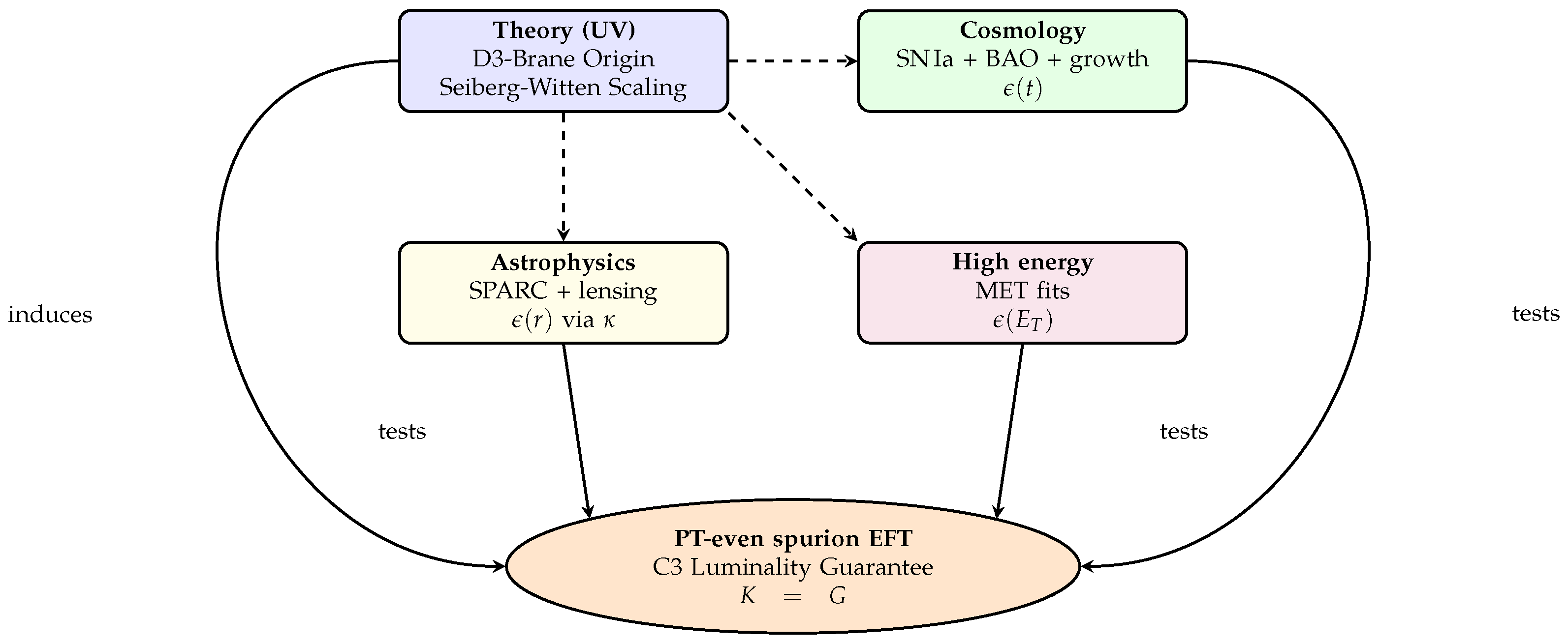
- UV Origin via D-Branes. While this work employs a bottom-up operator basis, the structure hints at a specific high-energy origin. The companion study [3] suggests that this PT-even Palatini action can be recovered from the low-energy limit of a Type-IIB D3-brane action subjected to a Seiberg-Witten scaling. In that context, the scalar spurion and the torsion trace arise naturally from the induced NS-NS two-form deformations, providing a string-theoretic candidate for the "flux" postulated here.
- 3.
- Beyond the current observational coverage. Cluster-scale lensing, BAO and growth constraints, and multi-messenger GW tests beyond baseline bounds remain to be incorporated in a uniform pipeline.
6.4. Roadmap
We conclude with a roadmap that matches the minimal-alignment strategy and scales naturally into a “fully consistent” series paper:
- R1: Consistency patch & reproducibility. Freeze parameter conventions and ensure tables/figures are generated from a single audited artifact.
- R2: Operator dominance by regime. Identify which PT-even operators dominate in FLRW, quasi-static galactic, and collider-like settings.
- R3: Toward first principles (D-Brane link). Explicitly derive the effective action coefficients from the Seiberg-Witten scaling limit of the D3-brane action, establishing the flux/spurion sector from string theory.
Figure 6.
Roadmap : The framework is grounded in a D-Brane UV origin and secured by the C3 Luminality Guarantee in the EFT core. Dashed arrows indicate the mapping from UV parameters to regime-specific templates.
Figure 6.
Roadmap : The framework is grounded in a D-Brane UV origin and secured by the C3 Luminality Guarantee in the EFT core. Dashed arrows indicate the mapping from UV parameters to regime-specific templates.
Acknowledgments and Data Availability
The author is grateful to the anonymous referees for comments that improved the manuscript.During the preparation of this work the author used OpenAI’s ChatGPT in order to perform limited language-level stylistic refinement and copyediting. After using this tool/service, the author reviewed and edited the content as needed and takes full responsibility for the content of the published article.
The Python code developed for the MCMC fitting procedure, model comparisons (PT-Symmetric Quaternionic, CDM, and MOND), statistical analysis, and figure generation presented in this work is openly available in a GitHub repository: https://github.com/ice91/PT-Quaternionic-Cosmology . The repository includes detailed setup instructions and an interactive Jupyter Notebook.
Funding
The author did not receive support from any organization for the submitted work.
Conflicts of Interest
Author Chien-Chih Chen is employed by Chunghwa Telecom Co., Ltd. The employer had no role in the study design, analysis, interpretation, decision to publish, or preparation of the manuscript. The author declares no competing interests.
Appendix A. PT-Even Projection, Selection Rules, and Variation–Projection Interchange
This appendix provides the structural backbone behind the PT-even “physical-sector” posture used throughout the minimal-alignment version of this paper. The main text introduces the PT-even projection operator in Equation (2.2), defines the physical action by projection in Equation (2.3) (equivalently Equation (1.1)), and states the variation–projection interchange rule in Equation (2.4). Here we (i) fix the PT action on the fields used in the Palatini/torsion EFT, (ii) record the key algebraic properties of the projector, (iii) state minimal sufficient conditions under which projection commutes with variation, and (iv) summarize the resulting PT-even selection rules that restrict the operator basis.
Appendix A.1. Definition of the PT Action in the Palatini/torsion Posture
Spacetime action.
We take the combined PT transformation to act on coordinates as
whose Jacobian is and hence . Therefore, the spacetime integration measure is preserved, and (for a real metric) is PT-invariant.
Antilinearity (time reversal).
In PT-symmetric constructions, the time-reversal operation is antilinear. Accordingly, we treat as an antilinear involution on (possibly complex) quantities: for complex numbers, includes complex conjugation, and for quaternion-inspired intermediate expressions one may take the corresponding conjugation. In the minimal-alignment posture adopted here, the physical metric and the spurion are taken to be real and PT-even, so the antilinearity plays no role in the final projected observables but is conceptually important for defining the projector.
Tensor transformation law.
For a generic tensor field that carries only spacetime indices, we define
where we used . Because , the Levi–Civita tensor density is PT-even. Hence, under the combined PT transformation, pseudo- versus polar-tensor distinctions do not introduce extra sign factors beyond the index-counting in Equation (A.2).
PT assignments of fields.
The minimal-alignment PT assignments used in the main text are:
The torsion tensor (defined in Equation (2.7)) then satisfies
and the torsion irreducible components defined in Equation (2.10), namely , , and , transform with the sign dictated by their number of spacetime indices (one index for ; three for ).
Appendix A.2. PT-even Projector and Its Algebraic Properties
We recall the PT-even projection operator defined in Equation (2.2): for any quantity X in the algebra of fields/expressions,
Idempotency.
Assuming on the bosonic sector used here, we have . Then
so .
Self-adjointness (with respect to a PT-invariant pairing).
Let denote any PT-invariant bilinear pairing compatible with the (real) spacetime measure, e.g.
or more generally a pairing for which . Then is self-adjoint:
because is the average of the identity map and a PT involution that preserves the pairing.
Reality of PT-even scalars.
In the minimal-alignment posture, the physical action and reported observables are defined by projection:
so only PT-even scalars contribute to . With the PT assignments in Equations (A.3)–(A.5), and the antilinear character of , PT-even projected scalars are real in the physical sector. This is the structural mechanism behind the “real observables by construction” claim emphasized in the main text.
Appendix A.3. Variation–projection Interchange
The main text states the variation–projection interchange rule
as the minimal consistency condition required for a standard variational principle on the PT-even physical sector. Here we record simple sufficient conditions.
Condition 1 (fixed PT assignment).
We assume the PT transformation rule is fixed at the level of the field space: the map does not depend on the dynamical fields in a way that would vary under . Concretely, the coordinate action (A.1) and the index transformation (A.2) are fixed, and the PT parities (even/odd) assigned in Equations (A.3)–(A.5) are not varied.
Condition 2 (commutation of variation with PT).
For any functional expression X built from the fields, we assume
This holds whenever is a linear functional variation acting on the fields and acts as a fixed (anti)linear map on those fields.
Derivation.
Using linearity of and (A.11),
which is exactly Equation (2.4).
Boundary conditions.
If the action differs by PT-odd total derivatives, the projection removes them in the bulk, but one must additionally impose PT-invariant boundary conditions to avoid leftover boundary contributions. In practice, the same boundary assumptions used to discard standard total derivatives in GR suffice here, provided the boundary data are chosen PT-even. This is consistent with the bookkeeping of boundary operators (e.g. ) in Table 1.
Appendix A.4. PT-even Selection Rules for the Operator Basis
Because the physical action is defined by projection (Equation (2.3)), only PT-even scalar operators survive in . This section summarizes the corresponding selection rules used implicitly in the operator-basis posture of Section 2.4.
Rule 1 (PT parity of building blocks).
With the PT action (A.2)–(A.7),
Consequently, any scalar built from an even number of PT-odd tensors is PT-even, while a scalar containing an odd number of PT-odd tensors is PT-odd and is projected out.
Rule 2 (minimal PT-even torsion scalars).
At quadratic order in torsion irreps, the standard PT-even scalar invariants are
which are precisely the bulk structures appearing in the minimal basis summarized in Equation (2.15) and Table 1. Spurion dressings such as remain PT-even since is PT-even.
Rule 3 (derivatives and total derivatives).
Covariant derivatives carry one spacetime index and thus flip sign under PT when acting on scalars through the coordinate map (A.1). Therefore, operators with an odd number of explicit derivative indices can be PT-odd unless their indices are fully contracted into PT-even combinations. A simple bookkeeping example is the boundary operator : it is PT-even as a fully contracted scalar built from two PT-odd objects ( and ), but it is a total derivative under standard conditions and hence does not affect bulk equations (as noted in Table 1).
Rule 4 (practical implementation in the EFT).
In practice, the PT-even projected operator-basis action in the main text, e.g. Equation (1.4) or Equation (2.19), should be read as:
Write down a candidate operator list in the torsion/connection sector, then keep only the PT-even scalars under , separating bulk from boundary terms.
This is the minimal operational definition that makes the model auditable and keeps all reported quantities in the real PT-even sector.
Remark (scope).
The selection rules stated here are sufficient for the minimal-alignment implementation of this preprint. A more complete companion-series treatment may refine the PT assignments for additional fields (spin currents, fermions, explicit parity-odd invariants, etc.) and can extend the operator catalog. None of those extensions are required for the three-regime template phenomenology presented in this paper.
Appendix B. Torsion Decomposition, Contorsion, and Irreducible Projectors
This appendix collects the standard torsion/contorsion identities and the irreducible (trace/ axial/traceless) projector algebra used implicitly in Section 2, especially Section 2.2. The purpose is purely kinematic/diagnostic: it fixes conventions, makes the projection operators explicit, and states a minimal “single-vector no-go” lemma that is useful when auditing a torsion operator basis.
Appendix B.1. Conventions and Basic Definitions
We work with a real metric and an independent connection as in the Palatini posture of Section 2. In the minimal-alignment framework we impose metric compatibility, Equation (2.8), so that the departure from Levi–Civita geometry is carried by contorsion, Equation (2.9).
Torsion is defined by Equation (2.7):
Its irreducible components are defined as in Equation (2.10):
and the remaining traceless tensor is defined by subtracting the trace and axial parts, subject to the constraints
Levi–Civita symbol vs. tensor (to avoid sign ambiguity).
Throughout this appendix, denotes the totally antisymmetric symbol (density) with . It is not assumed to be obtained by raising indices of with . With this convention one may consistently use the contraction identity
which matches the sign choices implicit in Equation (2.11). (If one instead uses the metric-raised Levi–Civita tensor, the axial-sector formulae acquire an overall sign; the projector structure below is unchanged.)
Component count.
In four dimensions, carries independent components. The irreducible split is
Appendix B.2. Contorsion and Its Algebraic Relation to Torsion
With metric compatibility, the connection decomposition in Equation (2.9) implies that contorsion is algebraically equivalent to torsion. A standard identity is
or, with all indices lowered,
Conversely,
Equations (B.6)–(B.8) are purely algebraic and hold independently of the dynamics/choice of PT-even operator basis.
Appendix B.3. Irreducible Decomposition and Explicit Projector Operators
The decomposition stated in Equation (2.11) can be written as an explicit projection of an arbitrary torsion tensor into three orthogonal subspaces:
where the trace and axial pieces are
Subtracting (B.10) and (B.11) from yields automatically satisfying the constraints (B.3).
Projectors acting on torsion tensors.
Let be any rank-3 tensor antisymmetric in . Define its trace and axial contractions by
Then the three projection operators , , and are defined by
Applied to , Equations (B.13)–(B.15) reproduce Equation (2.11) and identify .
Idempotence and mutual orthogonality.
With the convention (B.4), one verifies the standard projector identities (on the space of tensors antisymmetric in ):
Orthogonality under the natural inner product.
Define the (pointwise) inner product
Then the three components are orthogonal:
This orthogonality is what makes the trace/axial/traceless split a convenient “white-box” language for a torsion operator basis: quadratic invariants like , , and do not mix at the purely kinematic level.
Appendix B.4. A Minimal “Single-Vector No-Go” for the Traceless Sector
This lemma is useful when auditing operator ansätze that attempt to parameterize all torsion structure in terms of a single background vector (e.g. in FLRW) or a single radial unit vector in a static ansatz.
Lemma A1
(Single-vector no-go for ). Let be a single vector field. Consider tensors that are (i) antisymmetric in , and (ii) constructedlinearlyfrom using only and (no additional independent vectors/tensors and no derivatives). If satisfies the traceless-sector constraints (B.3), then .
Proof.
Under the stated assumptions, the most general linear ansatz built from a single vector and the available invariant tensors is a linear combination of the two independent structures:
since any term proportional to is symmetric in and hence drops out, and any -structure must contract its remaining index with to remain linear in V.
The first term in (B.19) is precisely a pure trace-type torsion: it has nonzero trace (up to signature conventions), so the constraint forces (unless ).
The second term in (B.19) is precisely a pure axial-type torsion: contracting with gives , so the constraint forces (again unless ).
Therefore and . □
Practical implication.
In a background where the only available vector is, for instance, the FLRW four-velocity , any torsion ansatz linear in can populate only the trace and/or axial sectors. A nontrivial traceless component requires additional structure (e.g. anistropy, multiple independent vectors, gradients/derivatives, or genuinely tensorial sources). This is why, in the minimal-alignment truncations used in Equation (3.2) and Equation (3.10), it is consistent (and often forced) to set the background .
Appendix B.5. Useful Identities for Operator Auditing
For quick reference, we list a few identities that are frequently used when reducing quadratic torsion invariants to irreducible components.
Reconstruction of qλμν .
From Equations (B.9)–(B.11),
Quadratic norm split.
Using orthogonality (B.18),
In terms of the vectors and , one finds (with the above convention)
so that the full quadratic invariant decomposes as
This identity is often useful when mapping between different conventions for a quadratic torsion basis.
Appendix B.6. Minimal Symbol Checklist (Local to Appendix B)
- : real physical metric (minimal alignment).
- : independent connection (Palatini posture).
- : torsion tensor (Equation (2.7)).
- : contorsion, (Equation (2.9)), with K–T relations (B.6)–(B.8).
- : trace torsion vector (Equation (2.10)).
- : axial torsion vector (Equation (2.10)).
- : traceless torsion component satisfying (B.3).
- : irreducible projectors (B.13)–(B.15) with algebra (B.16).
Appendix C. Measure, Reality, and (Optional) Quaternionic Determinants
This appendix clarifies the measure/reality issue in the minimal-alignment implementation adopted in the main text: the metric sector is taken to be real (and PT-even), while quaternion-inspired structure is carried by the independent connection (torsion/contorsion) and controlled by the PT-even projection principle. The key statement is that the physical action is defined by projection,
consistent with Equation (1.1) and the projector definition Equation (2.2). This construction fixes the reality of reported observables and, in the minimal posture, selects the standard real measure (Section 2.3).
Appendix C.1. PT-even Projection and the Physical Measure in Minimal Alignment
A frequent vulnerability of quaternionic/complexified-metric proposals is that a naive “determinant” does not define a unique real volume form, and the status of the variational principle becomes ambiguous once noncommutative operations are introduced. In the present paper we avoid this by a strict physical-sector rule:
The physical action and all reported observables are defined by the PT-even projection .
Concretely, for any scalar density that may contain non-real structures in an underlying formal expression, we define its physical content as
so that is PT-even by construction. In the minimal-alignment version used throughout the phenomenology sections, the physical metric is taken to be real (PT-even) and we adopt the standard volume form
identical to Equation (2.14). The physical action may therefore be written in the manifestly real form
where is the underlying (possibly non-real) Lagrangian density prior to projection, and the spurion normalization follows the main text.
Reality statement (what is guaranteed).
Equation (C.4) makes the central guarantee explicit: the reported integrand is PT-even, hence real in the physical sector, and the measure is real by construction. Quaternion-inspired structure is implemented through PT-even operator content in the torsion/connection sector, rather than by introducing a physical “imaginary metric”.
Scope statement (what is not attempted here).
The present work does not attempt to define a path integral over a genuinely quaternion-valued metric with a noncommutative measure. Such a UV completion can be pursued as an optional route (Appendix H in the planning blueprint), but it is not required for the minimal-alignment, template-level phenomenology presented in this paper.
Appendix C.2. Optional Route: Quaternionic Determinants and Projected Volume Forms
For readers interested in a more formal quaternionic measure, one may introduce a quaternionic determinant through a complex representation of quaternionic matrices, and then extract a real scalar density by PT-even projection. This subsection is optional and not used in fits or conclusions of the present minimal-alignment analysis.
Complex representation and a real “determinant”.
Let . Using the standard embedding ,
one obtains a complex matrix by applying entrywise. A standard construction (often called the Study/Dieudonné-type route in the physics literature) is to define a nonnegative real scalar
which is multiplicative and reduces to when A is complex-valued. (Different conventions exist; the essential point is that a representation-based prescription can produce a real scalar suitable for a volume-form candidate.)
Projected quaternionic volume form (formal).
If one insists on writing an underlying geometric object that is not manifestly real, a formal volume element could be defined as
so that the physical measure is explicitly PT-even. In the minimal-alignment posture of the main text, however, the physical metric is taken to be real and one simply has
recovering Equation (2.14) without invoking any quaternionic determinant technology.
Why this remains optional here.
Even with specified, a fully consistent quaternionic gravity theory requires additional structural choices (e.g. how curvature and variation are defined when noncommutativity is present). Since the present paper is explicitly minimal-alignment and diagnostic-first, we treat this determinant route as a future formalization option rather than as part of the data-facing model.
Appendix C.3. Why the Early “Hard Cut” Is Obsolete in the PT-even Framework
Early drafts sometimes attempted to enforce a real measure by an ad hoc replacement of the schematic form
where denotes a “real part” of a more general object G. This procedure is fragile: it does not follow from a symmetry principle, it obscures what is being projected out, and it can conflict with a controlled variational posture.
In the present formulation the measure issue is handled at the correct logical level: the physical sector is defined by the PT-even projection. The physical action is (Equation (1.1)), and the minimal-alignment implementation chooses a real physical metric and the standard measure (Equation (2.14)). Any non-real structures that may appear in an underlying formal expression are either: (i) removed from reported physics by , or (ii) relegated to the optional determinant route of Appendix C.2, which is explicitly not used in fits.
Practical takeaway.
Within the PT-even Palatini/torsion posture of this paper, one never needs to invoke Equation (C.9). The reality of the measure and observables is enforced by the physical-sector definition itself (projection), and the nontrivial “flux” content is carried in the torsion/connection operators that remain explicit and auditable in the effective action.
Appendix D. Template Definitions and Dimensional Consistency
This appendix collects the precise definitions of the three regime-dependent templates used throughout the minimal-alignment implementation: (cosmology), (galaxies), and (colliders). The purpose is threefold:
- 1.
- to fix notation and domains unambiguously;
- 2.
- to make dimensional/normalization choices explicit;
- 3.
- to state clearly what is and is not being claimed about cross-scale “unification” in this preprint.
Throughout we work with the reduced Planck mass and the normalization (Equations ((2.12), (5.1)). Unless stated otherwise, we set .
Appendix D.1. Template Definitions, Parameters, and Domains
Cosmology template ϵ(t).
The cosmic template used in Section 3.1 and Section 5.2 is (Equation (3.6))
with and dimensionless. This template is bounded, , and in late-time cosmology saturates toward . The associated scalar proxy field is defined by (Equation (3.7))
Galaxy template ϵ(r).
The quasi-static radial template used in Section 3.2 is (Equation (3.11))
with a length scale (fit or global scale depending on the analysis choice). For radial coordinate , this implies , and for . The corresponding proxy field is (Equation (3.11)).
Collider template ϵ(ET ).
In the high-energy analysis, the relevant kinematic variable is the missing transverse energy,
measured in GeV. The minimal-alignment philosophy treats the collider profile as a shape-level modulation template rather than as a UV-complete prediction.
For compactness, we collect the three regime templates in the form used in Equation (5.2):
where is dimensionless and is an energy scale (fixed in the reference implementation). In practice, the fit template used for the CMS spectrum is written directly at the level of the probability density (Equation (5.11)) as a bounded modulation . The relation between these two expressions is purely operational: Equation (D.5) summarizes the intended oscillatory kinematic imprint, while Equation (5.11) implements a normalized, positive-definite modulation appropriate for Poisson count data. No claim is made that a unique microscopic mapping fixes the precise functional prefactor across datasets (see Appendix D.3).
Appendix D.2. How Each Template Enters Observables
Appendix D.2.1. Cosmology: Background Torsion Amplitude and Effective Density Map
On an FLRW background, the minimal truncation encodes the PT-even torsion excitation through the trace vector aligned with the cosmological four-velocity (Equation (3.2)),
where has dimension of inverse time and is dimensionless. This makes dimensionally consistent with torsion, .
Because the present preprint defers a complete operator-audited mapping from the torsion basis to the background stress tensor, the net PT-even spurion imprint is packaged into an effective dark-sector density . The minimal mapping used in Section 3.1 is (Equation (3.8))
with the present cosmic time. This map is intentionally conservative: it preserves positivity and yields a -like late-time behavior when saturates. The corresponding effective equation of state is defined by Equation (3.5).
Appendix D.2.2. Galaxies: Radial Torsion Scale, Acceleration Scale, and Velocity Law
In the quasi-static galactic reduction, torsion is parameterized by a radial trace profile (Equation (3.10)),
so that , as required.
To map the geometric scale into a physical acceleration, the model introduces a dimensionless coupling , defining (Equation (3.12))
which has the correct units of acceleration when c is restored. Operationally, is the single amplitude controlling the spurion-induced galactic effect in the minimal template, and in a complete operator treatment it would be a derived combination of PT-even operator coefficients and environment dependence (cf. Equation (4.12)).
The rotation-curve template used in Section 3.2 takes (Equations (3.13)–(3.14))
The shape function is bounded and exhibits the expected limits: for (suppressed inner contribution) and for (outer scaling). In the outer region, this implies , reproducing the baryonic Tully–Fisher scaling at the level of the template.
Appendix D.2.3. Colliders: Normalized Modulation Template for Count Data
For the CMS spectrum, the comparison is performed with a binned Poisson likelihood and deviance (Equations (5.6)– (5.7)). The template used in the fit is expressed at the level of a positive, normalized shape (Equation (5.11)),
Here controls the exponential falloff scale, while controls the oscillatory modulation strength. The constant factor is a fixed normalization convention in the reference implementation, chosen so the template remains approximately normalized over the fit window; it is not treated as an additional physical parameter.
The role of in Equation (D.5) is therefore interpretational: it encodes the intended PT-even oscillatory imprint in a kinematic reduction. The actual data confrontation uses the bounded modulation in Equation (D.11), which is the appropriate object for Poisson count statistics and for ensuring positivity of the predicted spectrum.
Appendix D.3. What Is Not Claimed in Minimal Alignment
To prevent cross-regime over-interpretation, we state explicitly what this preprint does not claim.
- No single universal PDE across all scales. The three profiles , , and are treated as regime-dependent templates (Section 1.4 and Figure 5), not as the literal continuation of one unique equation of motion across many orders of magnitude.
- No unique operator-to-template derivation is asserted here. Although the framework is parameterized by a PT-even torsion operator basis, this preprint does not fix a complete catalog nor derive each template from a single audited operator subset. Environment- and scale-dependence is allowed through effective coefficients (Equation (4.12)), and the templates should be read as shape-level reductions of that sector.
- No UV-complete collider prediction is claimed. The collider analysis is a template-level shape test against public distributions. It is not presented as a first-principles prediction of new states, nor as a cross-scale extrapolation of the cosmological or galactic background equations.
- No cross-dataset universality of is assumed. Stability of the modulation parameters across selections/datasets is a falsifiability target (Section 5.6), not an assumption built into the minimal-alignment framework.
Appendix D.4. Notation and Dimensional Summary
For quick reference, Table A1 summarizes the primary template parameters and their dimensions.
Table A1.
Notation and dimensions used in Appendix D. We use natural units unless stated otherwise.
Table A1.
Notation and dimensions used in Appendix D. We use natural units unless stated otherwise.
| Symbol | Meaning | Dimension |
| reduced Planck mass | energy | |
| real scalar proxy (PT-even spurion) | energy | |
| dimensionless spurion amplitude | 1 | |
| Planck time (fixed) | time | |
| cosmic template steepness (fit parameter) | 1 | |
| galactic transition scale | length | |
| dimensionless coupling in | 1 | |
| effective acceleration scale | acceleration | |
| missing transverse energy | energy | |
| MET exponential falloff scale | energy | |
| MET oscillation scale (fixed in reference run) | energy | |
| MET modulation strength | 1 |
Consistency checks (quick).
With these conventions, in Equation (D.6) has dimension , in Equation (D.8) has dimension , and the collider template in Equation (D.11) is positive and normalizable over the fit range.
Naming convention.
We reserve as shorthand for (Equation (A45)), and we avoid ambiguous variants such as without a subscript. Similarly, we keep the reduced Planck mass notation consistent with the main text and do not use the unreduced GeV.
Appendix E. Diagnostics: Luminality, Stability, Fifth-Force Baselines, and Kerr Benchmarks
This appendix collects the diagnostic posture used throughout the minimal-alignment implementation: (i) the tensor-sector quadratic action and its luminality baseline, (ii) ghost/gradient stability conditions, (iii) the no-fifth-force baseline implied by minimal matter coupling, and (iv) benchmark estimates for Kerr-enhanced environments together with the mapping to observational bounds.
A recurring emphasis in this preprint is that the physical sector is defined by PT-even projection (Section 2.1), and that the nontrivial “flux/spurion” content is carried by the Palatini connection/torsion sector (Section 2.2), not by a physical imaginary metric. Consequently, diagnostics should be stated in standard EFT language (kinetic coefficients, stability inequalities, and observable mappings), and any speculative UV structure is kept optional (Appendix H).
Appendix E.1. Tensor-sector Quadratic Action in the PT-even Palatini/torsion EFT
Consider transverse-traceless tensor perturbations around a spatially flat FLRW background,
In a broad class of gravitational EFTs, after integrating out nondynamical fields and expressing the result in a gauge-invariant form, the quadratic tensor action can be written as
which matches the form already adopted in the main text, Equation (4.4). The tensor sound speed is then
consistent with Equation (4.5).
Why torsion-squared operators are “safe” at baseline.
In the minimal operator set used for this preprint (Table 1), the additional operators are quadratic in torsion irreps and are taken to be algebraic at leading order (no higher-derivative tensor kinetics are introduced). In such a truncation, torsion can be nondynamical in the tensor sector at quadratic order, so the spin-2 propagation is governed by the Einstein–Hilbert kinetic structure in with a real metric and PT-even projection. Put differently: the minimal basis is chosen so that any corrections to and arise only from (i) higher-dimension PT-even operators not included explicitly in the minimal set, or (ii) environment-dependent effective coefficients (Section 4.4.1), rather than from the mere presence of torsion-squared scalars.
Parametric form of corrections.
For bookkeeping it is useful to write
where encode PT-even corrections from operators beyond the pure Einstein–Hilbert baseline. PT-even projection ensures in the physical sector.
Appendix E.2. Luminality Baseline and Coefficient Bookkeeping
The baseline luminality diagnostic is the condition
identical to Equation (4.6) in the main text.
What is guaranteed vs. what is enforced.
In the companion-series posture (not reproduced here), one can impose a constructive condition on the operator basis such that a luminal tensor sector is guaranteed by a symmetry/identity. In the present minimal-alignment implementation, we adopt the weaker but defensible statement:
The operator subset explicitly retained in this preprint is chosen so that it does not generate higher-derivative tensor kinetics at leading order, and the remaining freedom (suppressed operators and environment-dependent effective coefficients) is constrained to satisfy the baseline condition (E.5) in the backgrounds to which we apply the templates.
Schematic coefficient constraint.
If a set of PT-even higher-dimension operators induces tensor-kinetic corrections, then to first order one may write
so that luminality requires
The key point for auditability is that the constraint is a linear relation among explicit Wilson coefficients once a concrete operator list is specified. In this preprint we do not claim a unique UV operator completion, but we keep the diagnostic interface explicit: any extension of the operator set must declare which combinations are set to zero and in which backgrounds.
Residual dispersion as “controlled deformation”.
When quoting a residual (Section 5), it is understood as arising from a suppressed operator combination that is not part of the baseline-enforced set, or from an environment-dependent effective coefficient that is not constant across regimes (Section 4.4.1). This is why the dispersion estimate is written parametrically in the main text, Equation (5.3).
Appendix E.3. Ghost and Gradient Stability Conditions
Stability diagnostics in the minimal-alignment posture follow standard EFT logic.
Appendix E.3.1. Tensor Sector
From Equation (E.2) one obtains the necessary conditions
which coincide with Equation (4.7) in the main text. In the baseline Einstein–Hilbert limit, , so the tensor sector is manifestly healthy.
Appendix E.3.2. Scalar Sector (Minimal Statement)
In a general Palatini/torsion EFT, additional scalar-like excitations may arise depending on which torsion irreps are promoted to dynamical fields and how they mix with . In the minimal-alignment implementation of this preprint, the dominant excitation used phenomenologically is a single PT-even scalar proxy (equivalently ), and scalar stability is summarized by
matching Equation (4.8). A fully explicit computation of requires fixing a concrete PT-even operator subset beyond the minimal list in Table 1; the minimal-alignment policy is therefore: we restrict attention to operator subsets for which (E.9) holds in the regimes where templates are applied, and we treat the remaining operator freedom as a controlled deformation space subject to diagnostics, rather than as an unconstrained “black box”.
Appendix E.4. No-fifth-force Baseline and Matter Couplings
The minimal-alignment version assumes that (spinless) matter couples minimally to the real metric ,
identical to Equation (2.6). This is the no-fifth-force baseline: test bodies follow the geodesics of in the Jordan frame, and any additional long-range force mediated by is absent at tree level because there is no direct coupling in .
Torsion and induced matter couplings.
In more general torsion theories, fermionic spin currents can source torsion and induce contact interactions after integrating out nondynamical torsion pieces. In the minimal-alignment posture, such effects are treated conservatively: if a nondynamical torsion component X couples linearly to a matter current, then integrating it out generates a suppressed effective operator, schematically as in Equation (4.11). This does not constitute a macroscopic fifth force for ordinary (spin-averaged) matter in the regimes considered here, but it does provide a clear audit target: any explicit inclusion of spin-coupled operators must be accompanied by an estimate of the induced scale and experimental bounds.
Practical diagnostic.
For the purposes of this preprint, “no fifth force” means: (i) the background and perturbation observables reported are computed with as in (E.10), and (ii) any induced matter coupling from torsion integration is assumed to be short-range or sufficiently suppressed in the considered datasets. This baseline is intentionally conservative and can be tightened in a fully audited operator completion.
Appendix E.5. Kerr Benchmarks and Mapping to Multi-Messenger Bounds
This subsection provides the benchmark logic behind the Kerr-related numbers quoted in the main text, and clarifies how residual estimates map to observational constraints.
Appendix E.5.1. Two Logically Distinct Effects
It is useful to separate two conceptually distinct notions:
- 1.
- Propagation along the cosmological path. Multi-messenger bounds constrain the path-averaged GW speed over cosmological distances. Under minimal alignment, the baseline diagnostic (E.5) is imposed in the propagation backgrounds used for cosmology, so the path-averaged deviation is taken to be negligible at leading order.
- 2.
- Localized strong-field environment near the source. Near a compact object (Kerr-like environment), environment-dependent effective coefficients (Section 4.4.1) could enhance suppressed operator combinations, producing a local residual dispersion target. Importantly, if such a deviation is confined to a small region of size around the source, its contribution to the total time delay is weighted only by , not by the full cosmological distance.
Appendix E.5.2. Benchmark Time-Delay Mapping
If a residual deviation is approximately constant over a region of physical size , the induced propagation delay is
For (with D the source distance), even a relatively large local can remain compatible with cosmological path-averaged constraints.
Appendix E.5.3. GW170817-style Bound (Order-Of-Magnitude)
A standard way to express the multi-messenger constraint is as a bound on the path-averaged speed difference:
where is the observed arrival-time offset and D is the luminosity distance. Using the well-known “ s versus million years” scale comparison yields an order-of-magnitude bound at the – level on a distance-averaged deviation. In the minimal-alignment posture, the baseline implementation sets this average to (effectively) zero at leading order by enforcing Equation (E.5) in the propagation regime.
Appendix E.5.4. Baseline Kerr Benchmark Used in This Preprint
To quantify a localized strong-field target, we introduce a benchmark spurion amplitude in a Kerr-like environment, denoted . In the conservative baseline quoted in the main text, we adopt
where is the gravitational radius of the compact object. This number is used as an input benchmark (not a claimed universal prediction) representing a strongly suppressed coupling between the torsion-sector spurion and curvature invariants in the Kerr environment.
The corresponding residual dispersion estimate is taken in the same parametric form as the main text, Equation (5.3), with . For the baseline benchmark (E.13), this yields the representative estimate quoted in the main text,
well below present dispersion sensitivities and safely compatible with multi-messenger propagation bounds even without invoking locality.
Consistency with multi-messenger bounds (locality argument).
Even if one considers a hypothetical larger local deviation near the source, its contribution to the observed time delay is suppressed by the small ratio via Equation (E.11). Thus, the conservative baseline benchmark (E.13) is safely consistent with multi-messenger constraints, and more aggressive local benchmarks (next subsection) are not automatically excluded provided they remain localized.
Appendix E.6. Optimistic Unsuppressed-Coupling Benchmark
For discovery-oriented forecasting it can be useful to define an optimistic benchmark in which the effective coupling is not Planck suppressed in the same way as the baseline. We therefore quote a separate, explicitly labeled scenario in which the Kerr environment can support a much larger effective amplitude,
as referenced in the main text (e.g. Table 5).
Using the same parametric dispersion estimator as in Equation (5.3) and the identification , one obtains the order-of-magnitude target quoted in the main text,
which would constitute a genuine strong-field dispersion signature if it can be realized consistently within an operator-complete PT-even basis while passing stability diagnostics.
Interpretation and caution.
This optimistic benchmark is not a claim of inevitability; it is a forecasting target illustrating what could become observable if environment-dependent effective coefficients are large in a localized region. Any serious use of this benchmark must specify: (i) which PT-even operators generate the enhancement, (ii) which stability conditions remain satisfied, and (iii) whether the deviation is localized (so that multi-messenger bounds are respected via Equation (E.11)).
Series-aligned “audit hook”.
The purpose of quoting both baseline and optimistic benchmarks is to provide an audit hook for the companion-series program: a fully specified operator basis should map curvature invariants into definite predictions for and for the induced in Equation (E.4), thereby turning the qualitative benchmarks (E.13) and (E.15) into quantitative, falsifiable targets.
Appendix F. Relation to Existing Frameworks and Operational Diagnostics
This appendix clarifies how the PT-even projected Palatini/torsion posture adopted in this preprint differs from several commonly discussed modified-gravity and torsion-based frameworks, and it summarizes the operational diagnostics that determine what is guaranteed, what is projected out, and what is only used at the template level.
Throughout, the physical sector is defined by the PT-even projection (Equation (2.2)) and the physical action rule (Equation (2.3) and Equation (1.1)), with the variation–projection interchange stated as a minimal consistency condition (Equation (2.4)). The metric sector is taken real and the “flux/spurion” content is carried by the independent connection through torsion/contorsion (Equations (2.7)–(2.9)) under metric compatibility (Equation (2.8)). Deviations from GR are parameterized by an explicit PT-even operator basis built from torsion irreducible components and boundary bookkeeping terms, summarized for the minimal truncation in Table 1 and the pipeline in Figure 1.
Appendix F.1. Minimal Operational Signature (What Is Fixed)
The minimal operational signature of this preprint is the conjunction of:
- 1.
- Physical-sector rule (reality by construction). Physical observables are defined by the PT-even projection (Equation (2.2)) acting on the underlying functional. Consequently, the physical action is PT-even and reported observables are real, by construction (Equation (2.3)).
- 2.
- Palatini posture with torsion as the flux carrier. The independent connection encodes the nontrivial structure via torsion (Equation (2.7)) and its irreducible decomposition (Equations (2.10)–(2.11)), with (Equation (2.9)). In the minimal-alignment implementation we impose metric compatibility (Equation (2.8)) and do not interpret an “imaginary metric” as a physical spacetime tensor.
- 3.
- White-box operator basis and diagnostics. Nonstandard effects are expressed as a finite PT-even operator list built from torsion irreps (Table 1) rather than a black-box curvature correction. This makes standard diagnostics (stability, luminality baselines, and fifth-force baselines) checkable.
- 4.
- Multi-regime templates are not a single universal PDE. The profiles , , and are treated as regime-specific templates representing kinematic reductions of the same PT-even spurion sector, with environment-/scale-dependent effective coefficients (see Section 4.4.1 and Figure 5).
Items (1)–(3) are structural and define the model class. Item (4) defines what is claimed (shape-level consistency across regimes) and what is not claimed (a single microscopic equation spanning all scales).
Appendix F.2. Relation to Common Frameworks
This subsection highlights where the present construction aligns with, or differs from, several well-known theory families. The intent is not exhaustive taxonomy, but an operational contrast: which degrees of freedom are used, how reality is enforced, and which diagnostics are built in.
Appendix F.2.1. Scalar–tensor EFTs (Horndeski/DHOST-type)
Scalar–tensor EFTs are typically formulated in a metric posture (Levi–Civita connection) with higher-derivative scalar interactions arranged to avoid Ostrogradsky instabilities (degeneracy conditions). A key historical discriminator was the tensor speed , since many scalar–tensor operators shift unless tuned or constrained.
In contrast, this preprint adopts: (i) a Palatini posture with an independent connection, (ii) torsion/contorsion as the carrier of the nontrivial spurion structure, and (iii) a baseline luminality diagnostic stated in the EFT tensor language (Equations (4.4)–(4.6)). Operationally, the statement is: the tensor sector is organized so that the baseline condition (hence ) can be enforced at leading order by coefficient/selection-rule control, rather than by hidden cancellations.
Appendix F.2.2. Einstein–Cartan / ECSK (Spin-Sourced Torsion)
Einstein–Cartan-type theories introduce torsion as an algebraic response to matter spin. In the simplest ECSK setting, torsion does not propagate and is sourced by fermionic spin currents; integrating it out yields contact interactions.
The minimal-alignment posture here shares the feature that torsion can be algebraic at leading order (given the quadratic torsion basis), but differs in what motivates and organizes the torsion sector: torsion is treated as a PT-even spurion/flux carrier with a projection-defined physical sector and an operator-basis diagnostic interface. In the spinless-matter baseline adopted in the main text (minimal coupling to ), torsion is not required to be sourced by spin currents, and its effective imprint is parameterized by -controlled operators (Table 1).
Appendix F.2.3. Teleparallel Gravity and Symmetric Teleparallel (Torsion/Nonmetricity Reformulations)
Teleparallel theories trade curvature for torsion by imposing a curvature-free connection, while symmetric teleparallel theories trade curvature for nonmetricity by imposing torsion-free but nonmetric connections. Both are reformulations of gravity in specific geometric gauges and often use distinct scalar invariants (e.g. torsion scalar T or nonmetricity scalar Q).
By contrast, the present framework: (i) does not impose vanishing curvature, (ii) keeps metric compatibility in the minimal truncation (Equation (2.8)), and (iii) uses torsion irreps inside an operator-basis EFT appended to rather than replacing R by T or Q. Operationally, this is a Palatini/torsion EFT around an Einstein–Hilbert baseline, not a curvature-free (teleparallel) gauge.
Appendix F.2.4. Chern–Simons Modified Gravity and Parity-Odd Extensions
Chern–Simons (CS) modified gravity introduces parity-odd curvature invariants (e.g. the Pontryagin density) coupled to a pseudoscalar. It generically implies parity violation in the tensor sector (birefringence/chiral GW propagation).
In the present work, PT-even projection is used as the physical-sector rule; PT-odd operators are projected out in (Section 2.1). Therefore, parity-odd curvature/torsion invariants can be discussed as optional structures but do not contribute to the reported physical action in the minimal-alignment posture. Operationally, the default prediction is the absence of parity-odd GW birefringence at leading order; any parity-odd signal would indicate either a different PT assignment, a different projection rule, or physics outside the minimal-alignment PT-even sector.
Appendix F.2.5. Metric-affine Gravity with Nonmetricity
General metric-affine theories allow both torsion and nonmetricity. The present minimal-alignment choice explicitly imposes metric compatibility (Equation (2.8)), thereby removing nonmetricity from the leading description. This restriction is a deliberate auditability choice: the operator basis is organized purely in terms of torsion irreps (trace/axial/traceless) so that selection rules and diagnostics are tractable.
Appendix F.2.6. Quaternionic/noncommutative UV Routes
Quaternionic and noncommutative geometry frameworks often require careful definitions of determinants, measures, and curvature functionals. In this preprint, such UV routes are treated as optional motivations and are not required for the minimal-alignment phenomenology. The physical-sector rule (Equation (2.3)) fixes the reality/measure issue at the EFT level (Equation (2.14)), while optional determinant constructions are deferred to future formalization (Appendix H in the planning blueprint).
Appendix F.3. Comparison Table (Operational Features)
Table A2 summarizes the most relevant operational differences.
Table A2.
Operational comparison with common frameworks. “This work” refers to the minimal-alignment PT-even Palatini/torsion posture in Section 2–Section 2.6.
Table A2.
Operational comparison with common frameworks. “This work” refers to the minimal-alignment PT-even Palatini/torsion posture in Section 2–Section 2.6.
| Framework | Geometric posture | Typical parity content | Operational discriminator |
| This work | Palatini, metric compatible; torsion irreps basis | PT-even projected physical sector (PT-odd projected out) | Real observables by construction (Equation (2.2)); explicit torsion-operator audit (Table 1); baseline tensor luminality diagnostic (Equation (4.6)) |
| Scalar–tensor EFT (Horndeski/DHOST) | Metric (Levi–Civita); scalar higher-derivative structure | Usually parity even; parity-odd variants exist | shifts unless tuned/constrained; degeneracy conditions; scalar fifth-force channels |
| Einstein–Cartan / ECSK | Metric + torsion; torsion sourced by spin currents | Parity even at baseline | Spin-contact interactions after integrating out torsion; torsion tied to matter spin |
| Teleparallel gravity | Curvature-free connection; torsion scalar T replaces R | Parity even at baseline | Reformulation via T; distinct boundary structure and field equations in teleparallel gauge |
| Chern–Simons modified gravity | Metric; parity-odd curvature invariant coupled to pseudoscalar | Parity odd by construction | GW birefringence/chirality at leading order; parity-odd propagation effects |
| Metric-affine (with nonmetricity) | Independent connection with torsion & nonmetricity | Model-dependent | Nonmetricity-driven observables; generalized geodesics; additional connection modes |
Appendix F.4. Operational Diagnostics Checklist
The “diagnostic-first” viewpoint of the main text can be made concrete as a checklist. The point is to make clear what a referee (or a reader) can verify in the minimal-alignment posture, and what is deliberately left as template-level.
Table A3.
Operational diagnostics: what is guaranteed (G), what is a baseline assumption (B), and what is template-level (T) in the minimal-alignment posture.
Table A3.
Operational diagnostics: what is guaranteed (G), what is a baseline assumption (B), and what is template-level (T) in the minimal-alignment posture.
| Diagnostic | Implementation in this work | Status |
| Reality of observables / measure | PT-even physical-sector rule; (Equations (2.2), (2.3)); standard volume form in (Equation (2.14)) | G |
| Variational well-posedness | Assume projection–variation interchange on the considered class of configurations (Equation (2.4)) | B |
| Degrees of freedom bookkeeping | Palatini posture with torsion irreps (Equations (2.7)–(2.11)); explicit operator list (Table 1) | G |
| No-fifth-force baseline | Matter minimally coupled to in the main text (Jordan frame baseline) | B |
| Tensor-sector luminality baseline | Quadratic tensor action in EFT form (Equation (4.4)); baseline condition so (Equation (4.6)) | B/G* |
| Ghost/gradient stability | Tensor conditions , and scalar analogs (Equations (4.7), (4.8)); operator subset restricted accordingly | B |
| Cross-regime unification claim | treated as regime templates with environment-dependent effective coefficients (Section 4.4.1, Figure 5) | T |
| UV completion / quaternionic measure | Explicit quaternionic determinants and noncommutative curvature calculus not required; deferred as optional route (planning blueprint Appendix H) | T |
* In the present minimal-alignment preprint, “baseline luminality” is achieved by restricting to operator subsets that do not introduce higher-derivative tensor kinetics at leading order (see the discussion around Table 1 and Equation (4.4)). In a fully audited series implementation one would derive the precise coefficient relations that enforce in a given background.
Appendix F.5. Boundary Terms and Equivalence Bookkeeping
Because the Palatini/torsion formulation naturally generates total derivatives and topological densities, it is important to separate (i) bulk operators that affect equations of motion from (ii) boundary terms used only for bookkeeping or for showing equivalences between operator parameterizations.
Appendix F.5.1. Generic Boundary Bookkeeping
A generic covariant divergence satisfies
so it does not affect bulk field equations under standard boundary conditions. In the minimal operator set we include a representative boundary term (Table 1) to keep track of such equivalences, while emphasizing that it is not used to generate the phenomenology.
Appendix F.5.2. PT-even Selection and Boundary Terms
A practical advantage of defining the physical action by PT-even projection is that parity-odd total derivatives and topological densities are automatically excluded from unless they have a PT-even component after projection. This makes the operational role of parity-odd boundary terms unambiguous in the minimal-alignment posture: they can be discussed as optional structures, but they do not contribute to the reported physical sector unless explicitly kept in PT-even form.
Appendix F.6. A Referee-Oriented “Decision Tree”
To avoid conflating optional motivations with minimal-alignment claims, it is useful to read the paper through the following decision tree:
- 1.
- Is the quantity PT-even? If yes, it can contribute to by Equation (2.2). If no, it is projected out and should not appear in the reported physical action.
- 2.
- Does it live in the metric sector or the connection sector? In minimal alignment, the metric is real and physical. “Flux/spurion” structure is carried in the connection/torsion sector (Equations (2.7)–(2.9)), not as a physical imaginary metric component.
- 3.
- Is it a bulk operator or a boundary bookkeeping term? Bulk operators affect dynamics; boundary terms are used only to track equivalences and do not affect bulk equations under standard boundary conditions (Equation (F.1)).
- 4.
- Does it pass the baseline diagnostics? At minimum, the tensor-sector baseline is organized around the EFT quadratic form (Equation (4.4)) and the luminality condition (Equation (4.6)), together with stability inequalities (Equations (4.7)–(4.8)).
- 5.
- Is the statement template-level or operator-derived? Results that rely on , , should be read as template-level phenomenology unless an explicit operator-to-observable mapping is provided (Section 4.4.1, Figure 5).
This decision tree is the operational expression of “series consistency”: the minimal-alignment preprint remains defensible by sharply separating (a) what is fixed by the PT-even projected Palatini/torsion posture from (b) what is used as a phenomenological template awaiting a complete operator-audited mapping.
Appendix F.7. Summary
In summary, the PT-even Palatini/torsion framework used here is best viewed as an auditable EFT posture rather than as a final UV-complete theory. Its distinctive operational features are: (i) a projection-defined physical sector that enforces real observables, (ii) connection/torsion as the flux carrier under a real metric sector, (iii) a white-box torsion-operator basis enabling standard diagnostics, and (iv) an explicit template-level interpretation across multiple regimes.
These features collectively explain why the model is structurally distinct from metric scalar–tensor EFTs, CS parity-odd modifications, teleparallel reformulations, and spin-sourced ECSK torsion, while still being compatible with standard gravitational diagnostics in the minimal-alignment sense.
Appendix G. Data, Likelihoods, Priors, and Reproducibility Artifacts
This appendix documents the public datasets, likelihood functions, priors, and reproducibility artifacts used in the minimal-alignment implementation of the PT-even projected Palatini/torsion spurion framework. The guiding principle is auditability: every figure and table quoted in the main text is linked to a deterministic Jupyter Notebook entry point and an explicit configuration record.
Conventions and normalization.
Unless stated otherwise we work in units and use the reduced Planck mass
consistent with the global definition used throughout the main text.
Appendix G.1. Pantheon SN Ia: Distance Modulus, Likelihood, Priors, and MCMC
This section corresponds to the Pantheon SN Ia analysis quoted in Section 5.2 and Figure A1 and Figure A2.
Figure A1.
Posterior distributions for from the Pantheon fit. Medians and 68% credible intervals correspond to Equation (5.5).
Figure A1.
Posterior distributions for from the Pantheon fit. Medians and 68% credible intervals correspond to Equation (5.5).
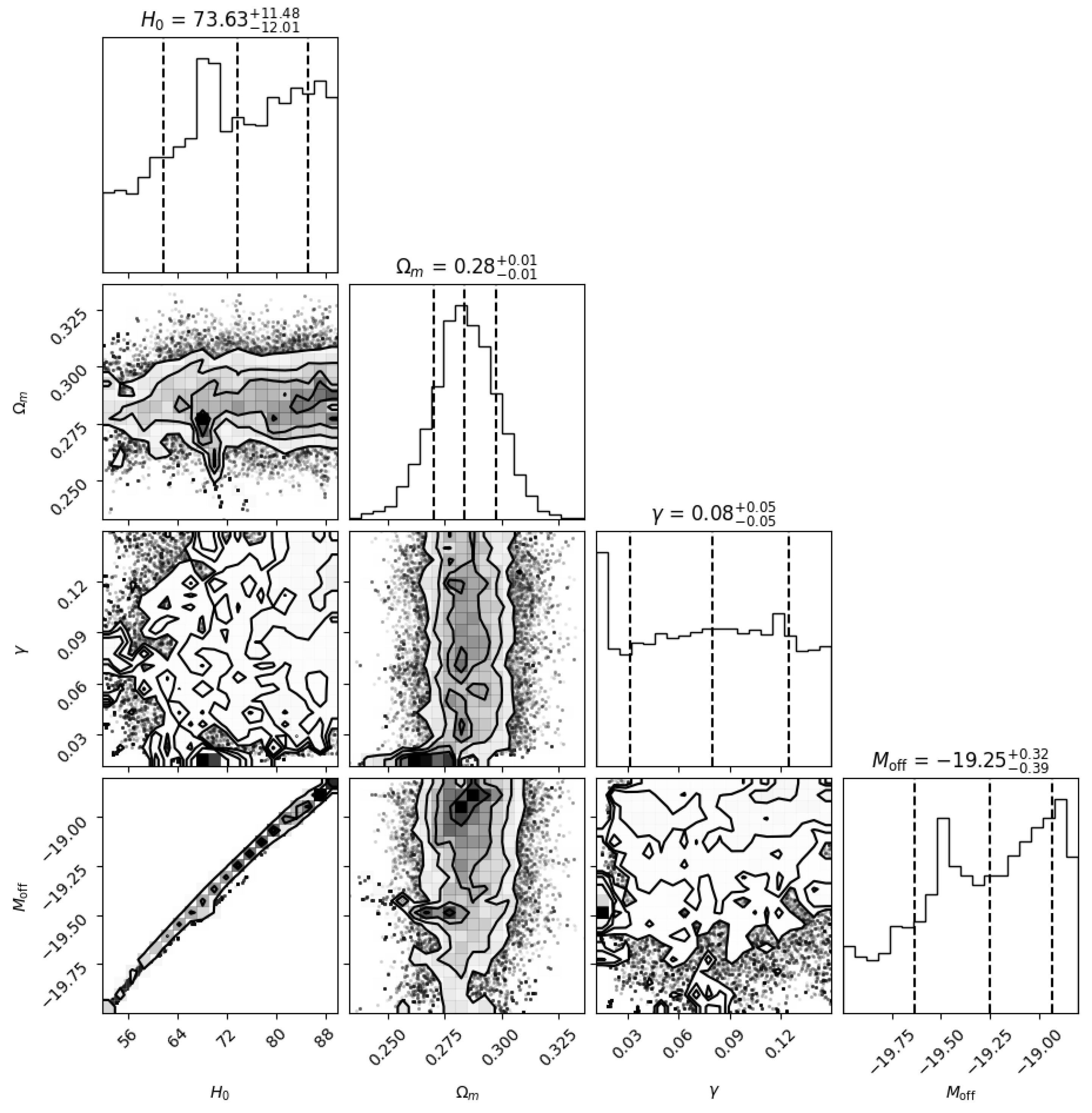
Figure A2.
Pantheon SN Ia Hubble diagram with the best-fit PT-even spurion template (solid line) and individual supernovae (points with errors).
Figure A2.
Pantheon SN Ia Hubble diagram with the best-fit PT-even spurion template (solid line) and individual supernovae (points with errors).
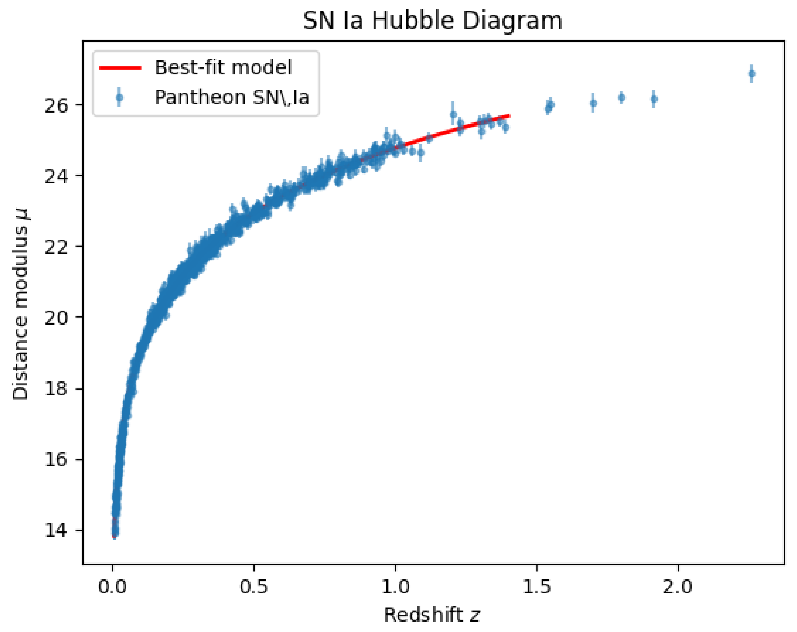
Dataset and Code
We use the Pantheon compilation ( SNe). The analysis is implemented in colab_notebooks/01_pantheon_sn_fit.ipynb. The notebook automatically fetches the standard release file (lcparam_full_long_zhel.txt) from the official repository.
Distance modulus model
For each supernova at redshift we compare an observed distance modulus to a model prediction , where the parameter vector is
The theoretical distance modulus is written as
with luminosity distance computed in a spatially flat FLRW background using the template .
Gaussian likelihood with full covariance
We use the standard Gaussian likelihood in terms of the residual vector and the Pantheon covariance matrix C:
The quoted goodness-of-fit in the main text is with and .
MCMC settings
The posterior is sampled using emcee (32 walkers, 5000 steps). Convergence is monitored within the notebook, and the summary statistics reported in Equation (5.5) correspond to posterior medians and central 68% credible intervals derived from the chain.
Appendix G.2. SPARC Rotation Curves: Model Definitions and AIC/BIC
This section documents the SPARC analysis referenced in Section 3.2 and Table 2. The implementation is provided in colab_notebooks/02_sparc_rotation_curves.ipynb.
Dataset
We use the SPARC rotation-curve catalogue (175 galaxies). The notebook expects individual galaxy files or a combined dataset.
Velocity models compared
For each galaxy we compare three templates: (i) Spurion: The saturating template added in quadrature to baryons. (ii) CDM: Standard NFW halo plus baryons. (iii) MOND: Simple interpolating function with acceleration scale .
Likelihood and metrics
For each galaxy g, we maximize a Gaussian likelihood (minimize ) via MCMC:
We report the reduced and the corrected Akaike Information Criterion (). The notebook generates the aggregate statistics table and exports the per-galaxy comparison to sparc_model_comparison.csv.
Appendix G.3. Compressed Early-Time Proxy Used in the Coarse Diagnostic Scan
This section documents the “compressed early-time proxy” used in the coarse grid scan. The calculation is performed in colab_notebooks/05_hubble_grid_scan.ipynb.
Sound-horizon proxy definition
We define the proxy sound horizon in the usual way (integral of sound speed over expansion history). In the coarse diagnostic scan we evaluate using the model implied by the template-level spurion mapping . We report the shift relative to a reference CDM value:
This proxy is used strictly as a directional diagnostic to verify that the parameter region interpolates consistently between regimes.
Appendix G.4. CMS Open Data: E T Miss Binning and Poisson Deviance Fits
This section documents the collider-template comparison in Section 5.5. The analysis is contained in colab_notebooks/04_cms_met_analysis.ipynb.
Dataset and selection
We use public CMS open data (fetched dynamically in the notebook) and construct a histogram of missing transverse energy on the range 0–500 GeV (50 bins).
Likelihood
We use the Poisson deviance to compare the standard exponential (CDM-like), power-law (MOND-like), and quaternionic modulation templates. The fit minimizes using scipy.optimize.curve_fit. The resulting best-fit parameters and the overlay plot (Figure 4) are generated directly by the notebook.
Appendix G.5. Released Artifacts and Figure-To-Notebook Map
To make the minimal-alignment results replayable, we map every major figure and table to the specific Jupyter Notebook that generates it.
Table A4.
Reproducibility map from quoted artifacts to deterministic notebook entry points.
| Artifact | Generated by (Notebook) |
| Figure A1 (Corner Plot) | colab_notebooks/01_pantheon_sn_fit.ipynb |
| Figure A2 (Hubble Diagram) | colab_notebooks/01_pantheon_sn_fit.ipynb |
| Table 2 (SPARC Statistics) | colab_notebooks/02_sparc_rotation_curves.ipynb |
| sparc_model_comparison.csv | colab_notebooks/02_sparc_rotation_curves.ipynb |
| Figure 4 (MET Spectrum) | colab_notebooks/04_cms_met_analysis.ipynb |
| Table 4 (Grid Scan) | colab_notebooks/05_hubble_grid_scan.ipynb |
| Kerr flux simulation ( verification) | colab_notebooks/03_kerr_flux_sim.ipynb |
Appendix G.6. Reproduce Via Notebooks
The analysis is structured as a series of independent Colab-ready notebooks. To reproduce the results:
- 1.
- Setup: Clone the repository and install dependencies (numpy, scipy, matplotlib, pandas, emcee, corner).
- 2.
-
Run Notebooks: Execute the notebooks in the colab_notebooks/ directory.
- 01_pantheon_sn_fit.ipynb: Generates SNIa constraints and figures.
- 02_sparc_rotation_curves.ipynb: Performs galaxy-by-galaxy MCMC fits.
- 03_kerr_flux_sim.ipynb: Verifies the Kerr-background flux solution.
- 04_cms_met_analysis.ipynb: Fits the collider missing energy spectrum.
- 05_hubble_grid_scan.ipynb: Runs the consistency grid check.
- 3.
- Data: All notebooks are configured to fetch necessary public data (Pantheon, SPARC, CMS) automatically or expect standard inputs in the data/ folder.
Appendix H. Optional Quaternionic / Noncommutative Route and Open Problems (Not Used in Fits)
Status and scope (read this first).
This appendix collects optional mathematical directions that may eventually provide a UV-facing or noncommutative foundation for the PT-even Palatini/torsion framework used in the main text. None of the constructions below are required for the minimal-alignment phenomenology, the likelihood fits, or the reported diagnostics. Throughout the paper, the physical sector is defined by the PT-even projection principle (Section 2, Equations (2.2)–(2.3)) and implemented with a real metric and the standard volume element (Equation (2.14)), while quaternion-inspired “flux” is carried by the independent connection/torsion sector (Equations (2.7)–(2.11)) with spurion amplitude (Equation ((2.12)). The purpose of Appendix H is therefore organizational: it states what could be pursued next, and what must be proven/defined before such statements can enter the main body.
Appendix H.1. Quaternion Algebra Basics (For Notation Only)
A quaternion is
with multiplication rules
Quaternionic conjugation is
and the (Euclidean) norm is
The real part is , and the imaginary vector part is .
Why this appendix needs these definitions.
Early drafts sometimes treated quaternionic objects (e.g. an “imaginary metric”) as directly physical. In the present minimal-alignment posture, this is not done: reality and the measure are fixed by the PT-even projection, and any quaternionic structure must flow into the PT-even operator content carried by torsion/connection (Section 2). Accordingly, Equations (H.1)–(H.4) are used only to define notation for optional UV routes discussed below.
Appendix H.2. Heuristic Quaternionic Coordinates and Their Non-Physical Role Here
For motivation it is sometimes convenient to write quaternionic-inspired coordinates
as a mnemonic for “extra internal directions”. In this paper, however, the components are not treated as physical coordinates, and no physical spacetime tensor is taken to be quaternion-valued. Instead, the intended effect of such extended structures is encoded by a single real spurion (or ) entering the PT-even torsion/connection sector (Equations (2.7)–(2.11)) after projection.
Minimal-alignment compatibility statement.
Equations like (H.5) are heuristic only and must not be read as implying that the physical volume element differs from Equation (2.14), or that the physical action is defined without projection. All physical variations and reported observables follow from the PT-even action (Equations (2.3) and (2.18)), together with the variation–projection interchange posture (2.4) adopted in Section 2.1.
Appendix H.3. Optional Route to Quaternionic Determinants and Measures
A common technical obstacle for quaternion-valued geometric objects is the definition of a determinant and hence a Lorentzian volume form. Minimal alignment avoids this issue by (i) defining the physical sector via the PT-even projection and (ii) choosing the physical metric to be real, yielding the standard measure (Equation (2.14)). Nevertheless, one may pursue an optional route in which a quaternionic determinant is defined through a complex representation.
Appendix H.3.1. Complex 2×2 Representation of H
Any quaternion can be written as
where denotes the usual complex numbers with imaginary unit . A standard faithful representation is
where the bar denotes complex conjugation in . One checks
Appendix H.3.2. Study/Dieudonn É-Type Determinants for Quaternionic Matrices (Optional)
For a quaternionic matrix , the map extends to a complex matrix . An often-used nonnegative determinant is the Study determinant
which is multiplicative on appropriate classes of quaternionic matrices. A related multiplicative construction is the Dieudonné determinant (also valued in for invertible matrices). These objects can be employed to define positive measures for Euclidean problems; Lorentzian signature introduces additional sign/phase subtleties.
PT-even measure proposal (future work; not used here).
If one insists on starting from a quaternionic-valued “metric-like” object , an optional proposal is to define a real physical volume element by projecting a determinant prescription to the PT-even sector:
Equation (H.10) is not implemented in this paper. The minimal-alignment implementation is instead Equation (2.14). A correct use of (H.10) would require specifying: (i) the class of quaternionic tensors allowed for , (ii) the determinant prescription and its invariance properties, and (iii) the precise PT action on consistent with (2.2). Until these are provided, (H.10) should be read only as a possible formalization target.
Appendix H.4. How a Quaternionic UV Picture Could Reduce to Palatini Torsion EFT
The main text encodes all nontrivial “flux” information in the torsion/connection sector (Section 2) rather than in a physical imaginary metric. A plausible UV-to-IR bridge (to be developed elsewhere) is that quaternionic or noncommutative degrees of freedom, once projected to the PT-even sector and integrated out (or coarse-grained), induce an effective Palatini/torsion action whose leading operators are precisely those built from torsion irreps (Equation (2.15) and Table 1).
Schematic bridge logic (informal).
One may imagine a more structured object (quaternionic frame, connection, or spectral data) whose PT-even projection yields:
with effective action coefficients emerging as low-energy Wilson coefficients. Under this viewpoint, the role of quaternionic structure is to motivate why torsion/connection can carry controlled PT-even invariants, while the physical implementation remains the PT-even projected EFT used in the paper.
What must be shown.
To turn (H.11) into a theorem-like statement, one would need to: (i) define the UV degrees of freedom and their PT action, (ii) define a UV measure (or show it reduces to Equation (2.14) after projection), (iii) show that the PT-even projected low-energy functional admits a Palatini posture with a well-defined torsion decomposition (2.11), and (iv) compute (or constrain) the induced operator basis and the sign/stability conditions of the resulting EFT.
Appendix H.5. Optional Noncommutative/Spectral Route (Conceptual Only)
A different optional foundation is a spectral or noncommutative construction in which geometry is encoded by algebraic data rather than by a metric tensor. In a conventional spectral setting one specifies data analogous to . A PT-even version would additionally require a well-defined PT action on the algebra and Hilbert space, and a projection rule that enforces PT-even reality for physical observables, mirroring (2.2).
Minimal-alignment compatibility.
Any such spectral route must, in the IR, reproduce: (i) a real physical measure consistent with Equation (2.14) (or a provably equivalent PT-even projection of a more general measure), (ii) the Palatini/torsion language used for auditability, and (iii) a coefficient-level operator basis that can be diagnosed (luminality, ghost/gradient stability) as in the main text. Until these conditions are met, spectral/noncommutative remarks should be kept outside the core appendices that support phenomenology.
Appendix H.6. Topology and K-theory Remarks (Strictly Speculative)
Topological or K-theoretic statements are particularly prone to over-claiming if the underlying bundle/connection/class is not explicitly defined. Accordingly, this subsection is purely speculative and is presented only as a list of possible future directions.
Speculative idea.
If the torsion/connection sector admits an effective reduction to a well-defined principal bundle connection A (or a higher-form generalization), then topological indices such as characteristic classes or index-theorem quantities could constrain discrete sectors of the spurion/flux background.
What cannot be claimed (in this paper).
Without specifying: (i) the precise bundle, (ii) the explicit connection A as a functional of (or of torsion irreps ), and (iii) the cohomology class being evaluated, one cannot assert concrete equalities between a “flux” parameter and a Chern class (e.g. formulas of the schematic form ). Therefore, any such statements must remain as conjectures with explicit assumptions.
Example conjectures (placeholders).
The following are examples of properly scoped conjectures:
- 1.
- (C-T1) Bundle definability conjecture: There exists a regime in which a PT-even combination of torsion components defines an effective connection on an auxiliary bundle, with gauge-invariant curvature .
- 2.
- (C-T2) Quantized sector conjecture: If (C-T1) holds and appropriate boundary/compactness conditions are satisfied, then for suitable closed 2-surfaces , yielding discrete “flux sectors”.
- 3.
- (C-T3) IR imprint conjecture: Discrete sectors (if present) map to restricted regions of EFT coefficient space , and hence restrict the admissible template families .
None of (C-T1)–(C-T3) is used in the fits or diagnostics of this paper; they are listed only to clarify what would need to be defined and proven.
Appendix H.7. Open Problems Aligned with the Minimal-Alignment Program
We conclude by listing open problems in a form aligned with the paper’s diagnostic-first posture.
H.1 Projection-level foundations
- 1.
- Provide a proof (or a sharply stated set of sufficient conditions) for the variation–projection interchange used in Equation (2.4), including boundary/regularity assumptions.
- 2.
- Specify the PT action on all geometric objects that may appear in an expanded operator basis (torsion irreps, covariant derivatives, curvature tensors in Palatini posture), and classify PT-even/odd operators systematically.
H.2 UV-to-IR mapping into an auditable operator basis
- 1.
- Construct an explicit UV model (quaternionic, spectral, or otherwise) whose PT-even projected IR limit yields a Palatini action with torsion operators, and compute the induced Wilson coefficients .
- 2.
- Demonstrate that baseline tensor-sector diagnostics (e.g. the luminality condition in the sense of Equation (4.6) in the main text) are automatically satisfied by symmetry/structure, or else quantify the degree of tuning required.
H.3 Template-to-operator mapping (the central missing link)
- 1.
- Derive (or tightly constrain) the mapping , including which operator subsets dominate in each regime and how environment dependence enters.
- 2.
- Replace the effective mappings used in the minimal-alignment fits by a single reproducible pipeline that propagates operator-level choices into observable-level predictions with shared priors and shared diagnostics.
H.4 Measure and determinant (only if one insists on quaternionic metrics)
- 1.
- If a quaternionic “metric-like” object is retained in a UV completion, define a Lorentzian measure unambiguously (e.g. via a determinant prescription) and show that PT-even projection yields a real functional weight consistent with the phenomenological sector.
- 2.
- Prove invariance properties of the chosen determinant under the relevant coordinate/frame transformations, and clarify how curvature and variation are defined in the noncommutative setting.
Pragmatic takeaway.
Minimal alignment deliberately avoids the measure and noncommutativity pitfalls by enforcing PT-even reality at the level of the physical action and by encoding flux in torsion/connection. Appendix H clarifies how one might restore a quaternionic or noncommutative UV narrative without destabilizing the auditable EFT posture of the main text: any such restoration must reduce to the PT-even projected Palatini/torsion operator basis as the IR, and must preserve the diagnostic interface that motivates the framework.
References
- C.-C. Chen, “Guaranteed Tensor Luminality from Symmetry: A PT-Even Palatini Torsion Framework,” Symmetry 18, no. 1, 170 (2026). [CrossRef]
- C.-C. Chen, “From Quaternionic Spacetime to MOND: A Single ϵ Anchored to H0 Links Galaxies and Cosmology,” Preprints 2025, 2025032052 (2025). [CrossRef]
- C.-C. Chen, “A D-Brane-Induced Quaternionic and PT-Symmetric Spacetime with Falsifiable Signatures,” Preprints 2025, 2025072429 (2025). [CrossRef]
- A. Einstein, Die Feldgleichungen der Gravitation, Sitzungsber. Preuss. Akad. Wiss. (Berlin) 1915, 844–847 (1915).
- P. A. M. Dirac, The Principles of Quantum Mechanics, Oxford University Press, 1st ed. (1930).
- A. Friedmann, “Über die Krümmung des Raumes,” Z. Phys. 10, 377–386 (1922).
- G. Lemaître, “A homogeneous Universe of constant mass and increasing radius accounting for the radial velocity of extragalactic nebulae,” Mon. Not. R. Astron. Soc. 91, 483–490 (1931).
- H. Weyl, “Quantenmechanik und Gruppentheorie,” Z. Phys. 46, 1–46 (1927).
- M. Milgrom, “A modification of the Newtonian dynamics as a possible alternative to the hidden mass hypothesis,” Astrophys. J. 270, 365–370 (1983).
- D. Finkelstein, J. M. Jauch, S. Schiminovich and D. Speiser, “Foundations of quaternion quantum mechanics,” J. Math. Phys. 3, 207–220 (1962).
- L. P. Horwitz and L. C. Biedenharn, “Quaternion quantum mechanics: Second quantization and some extensions,” Ann. Phys. 157, 432–488 (1984).
- E. Witten, “String theory dynamics in various dimensions,” Nucl. Phys. B 443, 85–126 (1995).
- A. Connes, “Noncommutative geometry and reality,” J. Math. Phys. 36, 6194–6231 (1995).
- S. L. Adler, Quaternionic Quantum Mechanics and Quantum Fields, Oxford University Press (1995).
- M. F. Atiyah, K-Theory, W. A. Benjamin (1967).
- D. D. Joyce, Compact Manifolds with Special Holonomy, Oxford University Press (2000).
- J. Madore, An Introduction to Noncommutative Differential Geometry and its Physical Applications, 2nd ed., Cambridge University Press (1999).
- C. Rovelli, Quantum Gravity, Cambridge University Press (2004).
- A. Ashtekar, T. Pawlowski and P. Singh, “Quantum nature of the big bang: Improved dynamics,” Phys. Rev. D 74, 084003 (2006).
- D. Clowe et al., “A direct empirical proof of the existence of dark matter,” Astrophys. J. Lett. 648, L109–L113 (2006).
- C. M. Bender, “Making sense of non-Hermitian Hamiltonians,” Rep. Prog. Phys. 70, 947–1018 (2007).
- B. P. Abbott et al. (LIGO Scientific Collaboration and Virgo Collaboration), “GW170817: Observation of gravitational waves from a binary neutron star inspiral,” Phys. Rev. Lett. 119, 161101 (2017).
- F. Lelli, S. S. McGaugh and J. M. Schombert, “SPARC: Mass models for 175 disk galaxies with Spitzer photometry and accurate rotation curves,” Astron. J. 152, 157 (2016).
- D. Foreman-Mackey, D. W. Hogg, D. Lang and J. Goodman, “emcee: The MCMC hammer,” Publ. Astron. Soc. Pac. 125, 306–312 (2013).
- D. M. Scolnic et al., “The complete light-curve sample of spectroscopically confirmed SNe Ia from Pan-STARRS1 and cosmological constraints from the Pantheon sample,” Astrophys. J. 859, 101 (2018).
- Planck Collaboration, “Planck 2018 results. VI. Cosmological parameters,” Astron. Astrophys. 641, A6 (2020).
- CMS Collaboration, “Search for new physics in events with missing transverse momentum and a Higgs boson decaying to two photons in proton–proton collisions at √s = 13 TeV,” J. High Energy Phys. 11, 152 (2019).
| 1 | Allowing an axial background is possible, but would introduce additional operators in the PT-even basis. The present choice is the minimal truncation consistent with isotropy. |
| 2 | A compact technical summary of the individual fits, likelihood functions, priors, and data sources is collected in Appendix G. |
| 3 |
Figure 1.
PT-even physical-sector pipeline adopted in this work. The PT-even projection defines the physical action and enforces real observables. Crucially, the diagnostic phase includes the C3 coefficient-locking identity which guarantees . Deviations from Einstein–Hilbert are parameterized by an operator basis built from torsion irreducible components and audited via standard diagnostics.
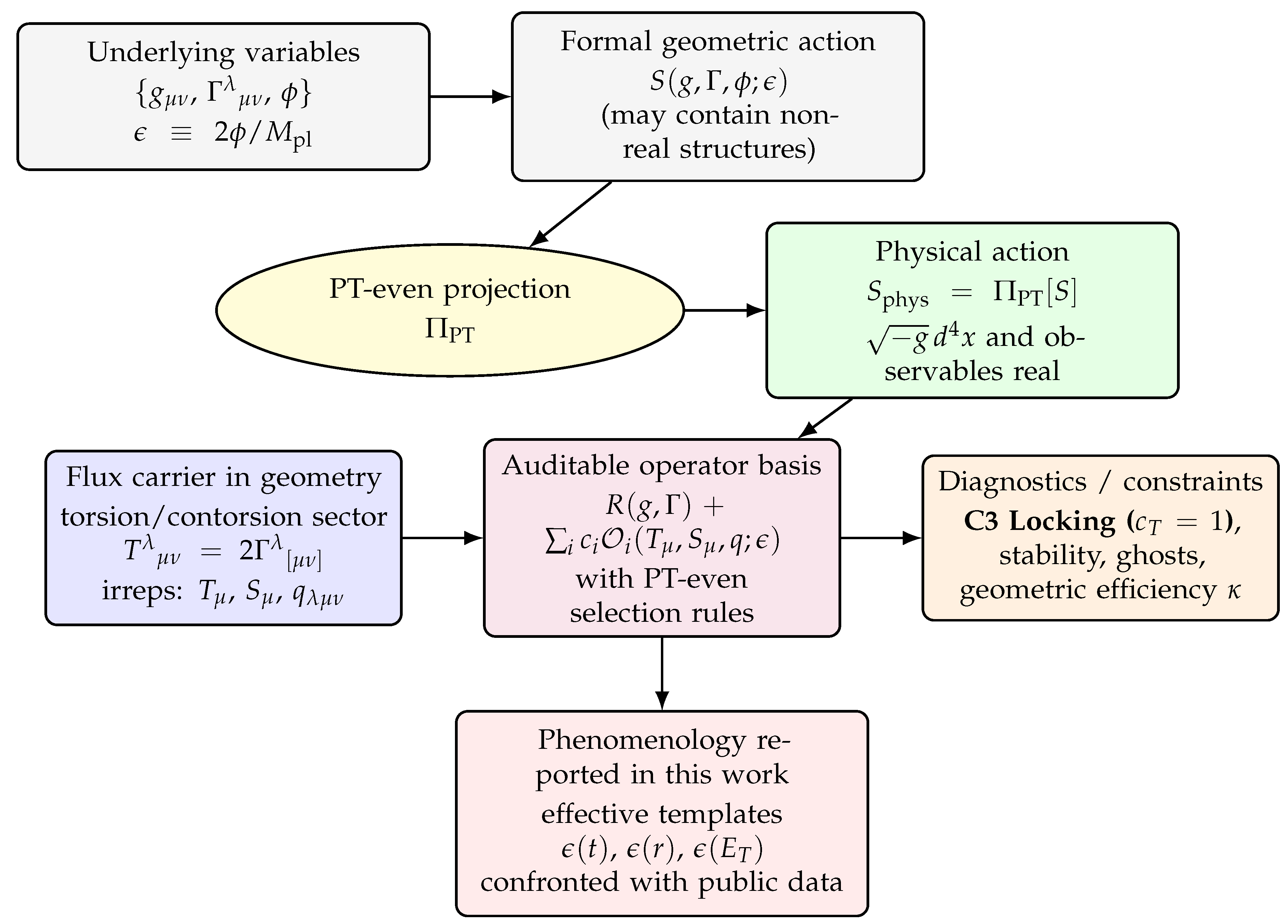
Figure 2.
Three-regime minimal-alignment interpretation. The spurion sector is common, but its observable imprint is represented by regime-dependent effective templates. Note the galactic template is controlled by a geometric efficiency factor , linking the effective acceleration to galactic morphology.
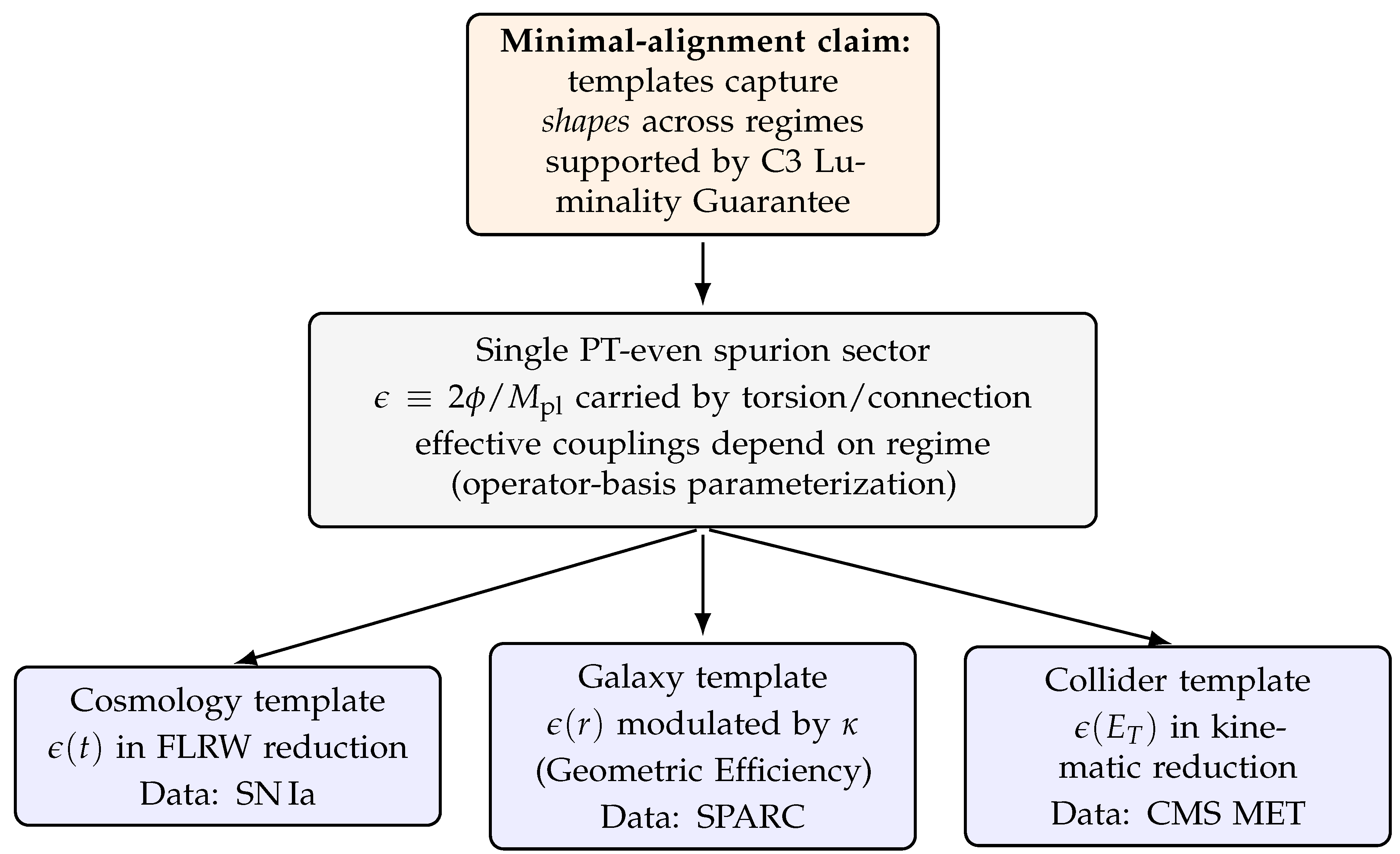
Figure 3.
Schematic evolution of the effective dark-energy density in the minimal-alignment mapping (3.8). Inset: the template of Equation (3.6), which saturates at late times.
Figure 3.
Schematic evolution of the effective dark-energy density in the minimal-alignment mapping (3.8). Inset: the template of Equation (3.6), which saturates at late times.
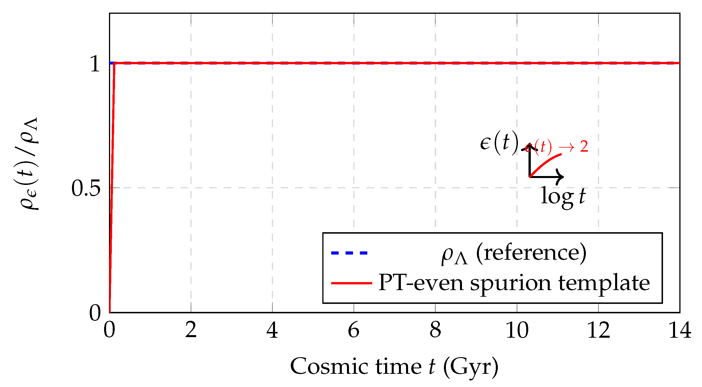
Figure 4.
CMS spectrum (points with errors) and best-fit templates. The PT-even spurion modulation template captures the shoulder structure more accurately than the pure exponential or pure power-law shapes (Appendix G.4).
Figure 4.
CMS spectrum (points with errors) and best-fit templates. The PT-even spurion modulation template captures the shoulder structure more accurately than the pure exponential or pure power-law shapes (Appendix G.4).
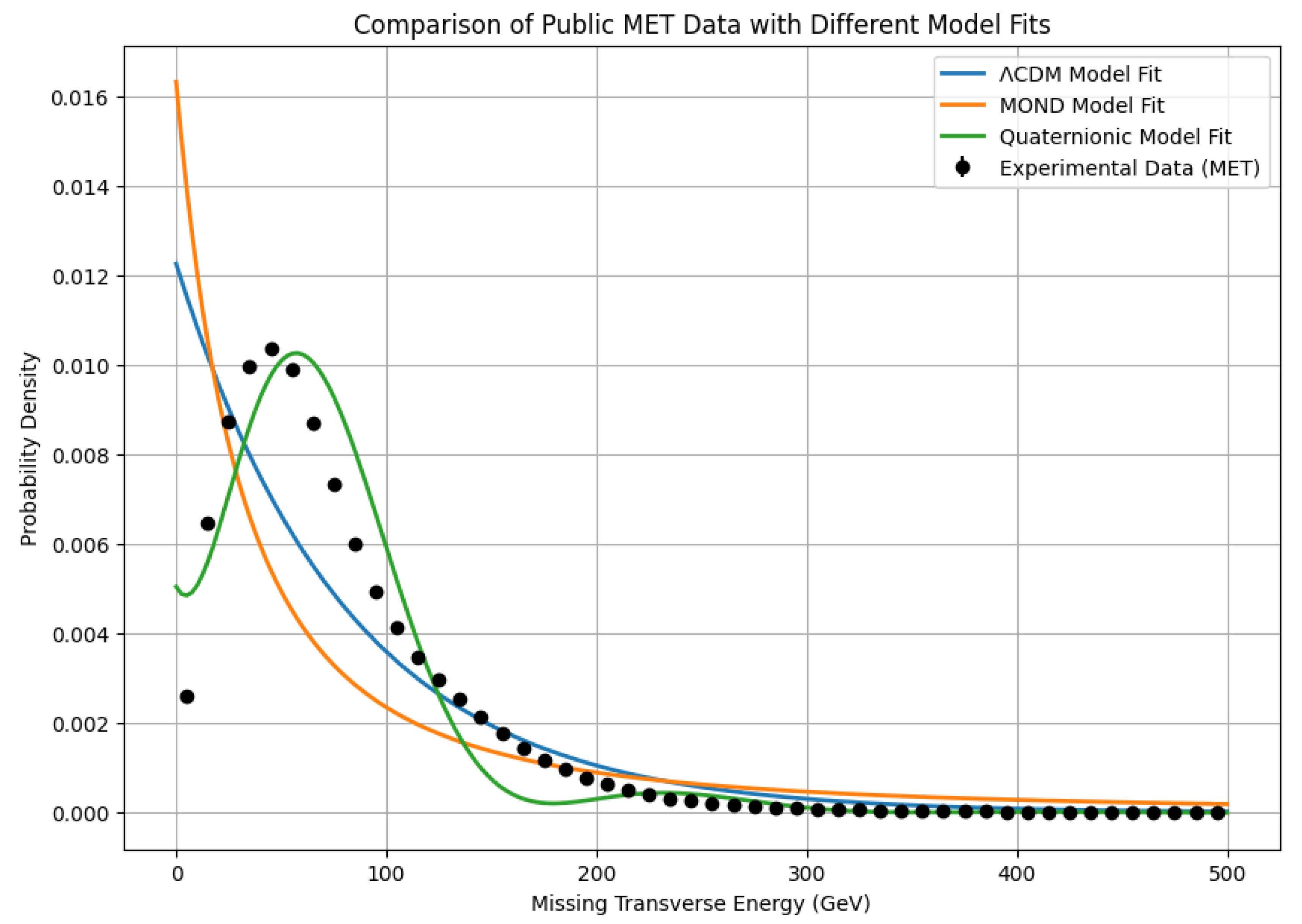
Figure 5.
Minimal-alignment logic: a single PT-even operator-basis spurion sector is reduced to regime-specific templates , , and , with environment-dependent effective coefficients and shared PT-even diagnostics.
Figure 5.
Minimal-alignment logic: a single PT-even operator-basis spurion sector is reduced to regime-specific templates , , and , with environment-dependent effective coefficients and shared PT-even diagnostics.
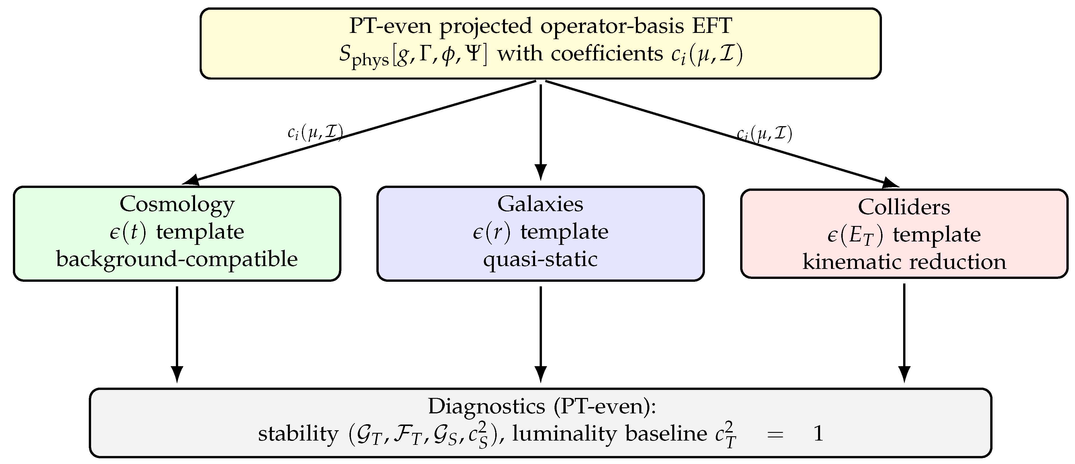
Table 1.
A minimal PT-even operator set replacing the black-box . The bulk operators are quadratic in torsion irreps and dressed by to emphasize the spurion-controlled amplitude. Boundary terms can be kept to track equivalences but do not affect bulk equations under standard boundary conditions.
Table 1.
A minimal PT-even operator set replacing the black-box . The bulk operators are quadratic in torsion irreps and dressed by to emphasize the spurion-controlled amplitude. Boundary terms can be kept to track equivalences but do not affect bulk equations under standard boundary conditions.
| Label | Operator (PT-even scalar) | Notes |
| bulk, algebraic torsion sector | ||
| bulk, PT-even after projection | ||
| bulk, traceless sector control | ||
| boundary / total derivative (bookkeeping) |
Table 2.
Aggregate performance on the full 175-galaxy SPARC sample. Columns show the sum, mean, and median of the reduced chi-squares, plus the number of galaxies for which each model yields the lowest AIC. (Values are reported for the current reference dataset/pipeline; see Appendix G for implementation details.)
| Model | Mean | Median | AIC best (N) | |
| Spurion (PT-even) | 73 | |||
| CDM | 92 | |||
| MOND | 10 |
Table 5.
Spurion amplitudes and their core observables. Baseline values correspond to the Kretschmann + Planck–suppressed coupling; optimistic values (in parentheses) assume an unsuppressed coupling as discussed in Appendix E.6.
Table 5.
Spurion amplitudes and their core observables. Baseline values correspond to the Kretschmann + Planck–suppressed coupling; optimistic values (in parentheses) assume an unsuppressed coupling as discussed in Appendix E.6.
| Regime | Spurion template | Benchmark amplitude | Core observable |
| Cosmic late time () | SN Ia distances | ||
| CMB era () | early-time expansion proxies | ||
| Galactic ( kpc) | (template) | rotation curves | |
| Kerr BH () | GW dispersion target | ||
| Collider tail ( GeV) | CMS MET shape |
Disclaimer/Publisher’s Note: The statements, opinions and data contained in all publications are solely those of the individual author(s) and contributor(s) and not of MDPI and/or the editor(s). MDPI and/or the editor(s) disclaim responsibility for any injury to people or property resulting from any ideas, methods, instructions or products referred to in the content. |
© 2026 by the authors. Licensee MDPI, Basel, Switzerland. This article is an open access article distributed under the terms and conditions of the Creative Commons Attribution (CC BY) license (http://creativecommons.org/licenses/by/4.0/).
Copyright: This open access article is published under a Creative Commons CC BY 4.0 license, which permit the free download, distribution, and reuse, provided that the author and preprint are cited in any reuse.


