Submitted:
21 February 2025
Posted:
24 February 2025
You are already at the latest version
Abstract
To address the issues of the current nodal pricing mechanism, which does not incorporate fixed transmission costs and leads to unfair transmission cost allocation, this paper proposes a full-cost electricity pricing model based on power flow tracing technology. By defining full-cost electricity pricing and integrating generation marginal costs with effective transmission costs, the proposed model adheres to the principle of "costs borne by beneficiaries." The effectiveness of the proposed model is validated through case studies on IEEE 30-bus and IEEE 118-bus systems. The results demonstrate that the proposed method can optimize power grid resource allocation and enhance investment efficiency while considering power grid congestion.
Keywords:
power flow tracing technology
; inter-provincial electricity trading
; power grid congestion
; transmission cost allocation
; security-constrained economic dispatch
; demand response
1. Introduction
With the deepening of electricity market reform, the efficiency and fairness of power grid resource allocation have become central issues in electricity market research. The current nodal pricing system typically considers only the marginal cost of generation while neglecting fixed transmission costs, leading to incomplete price signals that fail to reflect the actual utilization of grid resources by the load[1]. Additionally, traditional transmission cost allocation mechanisms lack scientific rigor and fairness, suppressing the potential of demand-side response and potentially inducing inefficient expansion of the transmission network, thereby reducing overall grid efficiency.
In recent years, scholars have conducted extensive research on nodal pricing systems and transmission cost allocation, achieving significant progress. Regarding nodal pricing: the marginal-cost-based nodal pricing system has been widely applied, but it generally assumes an uncongested transmission network, overlooking the impact of fixed transmission costs on nodal prices [2,3,4]. Some studies have proposed improved models that incorporate fixed transmission costs into electricity pricing [5,6]; however, they lack a mechanism to distinguish between effective and ineffective transmission costs, leading to inaccurate price signals[7].
Regarding transmission cost allocation: power flow tracing technology is regarded as an important tool for reasonably allocating transmission costs. It traces the distribution of power flows between generation and load nodes, clarifying each node’s contribution to line flows. However, most existing studies adopt postage stamp or average allocation methods, failing to fully capture the differences in grid resource utilization among nodes [8,9,10,11].
Regarding demand response and grid congestion research: as a crucial means of improving grid resource utilization efficiency, demand response has received widespread attention in recent years [12]. However, under the current electricity pricing mechanism, price signals fail to incentivize load-side adjustments in electricity consumption behavior, limiting the effectiveness of demand response. At the same time, grid congestion is often simplified in many studies, without fully reflecting its impact in pricing models.
To address the above issues, this paper proposes a full-cost electricity pricing model based on power flow tracing technology and designs a trading network model suitable for the spot market under the constraints of inter-provincial AC grid congestion. The main contributions of this study include:
- Proposing the concept of full-cost electricity pricing, which integrates generation marginal costs and effective transmission costs, addressing the deficiencies in the current nodal pricing system.
- Refining the transmission cost allocation mechanism using power flow tracing technology and establishing a price signal system based on the principle of “costs borne by beneficiaries.”
- Validating the model’s effectiveness in optimizing power grid resource allocation, alleviating grid congestion, and enhancing investment efficiency through case studies.
2. Materials and Methods
2.1. Fundamental Concept of Full-Cost Electricity Pricing
The current nodal pricing system does not incorporate transmission costs. Under the assumptions of a lossless DC power flow and an uncongested network, nodal prices remain uniform across different locations, failing to accurately reflect the impact of full generation and transmission costs on the spatial and temporal distribution of load. Additionally, traditional transmission cost allocation mechanisms do not distinguish between effective and ineffective transmission costs, making it difficult for the allocation results to truly reflect the utilization of grid resources by the load. This inefficiency in cost allocation negatively affects grid investment efficiency and contradicts the principles of optimal resource allocation [13,14].
To address these issues, this paper introduces the concept of full-cost electricity pricing, which integrates generation marginal costs with effective transmission costs [15,16,17,18]. By employing power flow tracing techniques, the proposed pricing model reasonably allocates fixed transmission costs, ensuring that electricity prices dynamically reflect the extent to which loads utilize grid resources while adhering to the principle of "costs borne by beneficiaries." Effective transmission costs are further classified into regular operational costs, N-1 security operational costs, future load growth costs, and ineffective transmission costs, ensuring that pricing signals remain fair and accurate while truly reflecting the actual cost of grid resource utilization by loads.
This paper defines the permitted cost recovery rate of transmission line at time as follows:
where:
In these equations:
is the capacity of transmission line .
represents the base-case power flow of transmission line .
is the maximum absolute value of the power flow on transmission line across the base case and all N-1 contingency scenarios.
The effective fixed transmission cost of transmission line at time is then calculated as:
where: represents the total transmission investment cost of line .
2.2. Derivation of Full-Cost Electricity Pricing Based on Power Flow Tracing Method
The power flow tracing method is a technique used to allocate the utilization of grid resources by generation and load nodes by analyzing power flow paths within the grid. In electricity markets, power flow tracing is widely applied to distribute transmission costs and identify the contribution relationships among grid resources. The fundamental assumption of this method is that the power injected at a node is fully mixed, and the power flowing out of a node is proportionally shared among the downstream branches. This method ensures both transparency in grid resource utilization and fairness in cost allocation.
Assuming that the power injected into and withdrawn from node e satisfies the following balance equation:
where: is the total injected power at node ; is the load power at node ; denotes the set of lines where node is the upstream node; is the power flow on transmission line .
Rearranging the equation:
Expressed in matrix-vector form, the backward flow tracing equation is given as:
Where is the backward flow tracing matrix, which represents the power flow distribution in the reverse direction. The elements of are defined as:
If is invertible, the node injection power vector can be obtained as:
where the –th element of the vector is:
For power flow allocation on line , the contribution of load node to the power flow on this line can be computed using the elements of the inverse backward flow tracing matrix :
Furthermore, the total contribution of node to the power flows across all transmission lines in the grid can be obtained by summing over all transmission lines. Combining this with the effective transmission cost , the total transmission cost borne by node can be expressed as:
where:
represents the total transmission cost borne by node ;
is the total investment cost of transmission line ;
is the permitted fixed transmission cost recovery rate of the line.
The unit transmission cost at node s then calculated as:
This unit transmission cost explicitly reflects the utilization of transmission network resources by each load node.
Finally, the full-cost electricity price at node is obtained by linearly combining generation costs and transmission costs:
where:
represents the marginal generation cost at node ;
is the unit transmission cost component.
The full-cost electricity pricing model allocates total grid costs based on power flow tracing, reflecting differences in grid utilization due to the spatial distribution of loads. This approach ensures that nodes bear differentiated generation and transmission costs, leading to a more equitable and efficient electricity pricing system [19].
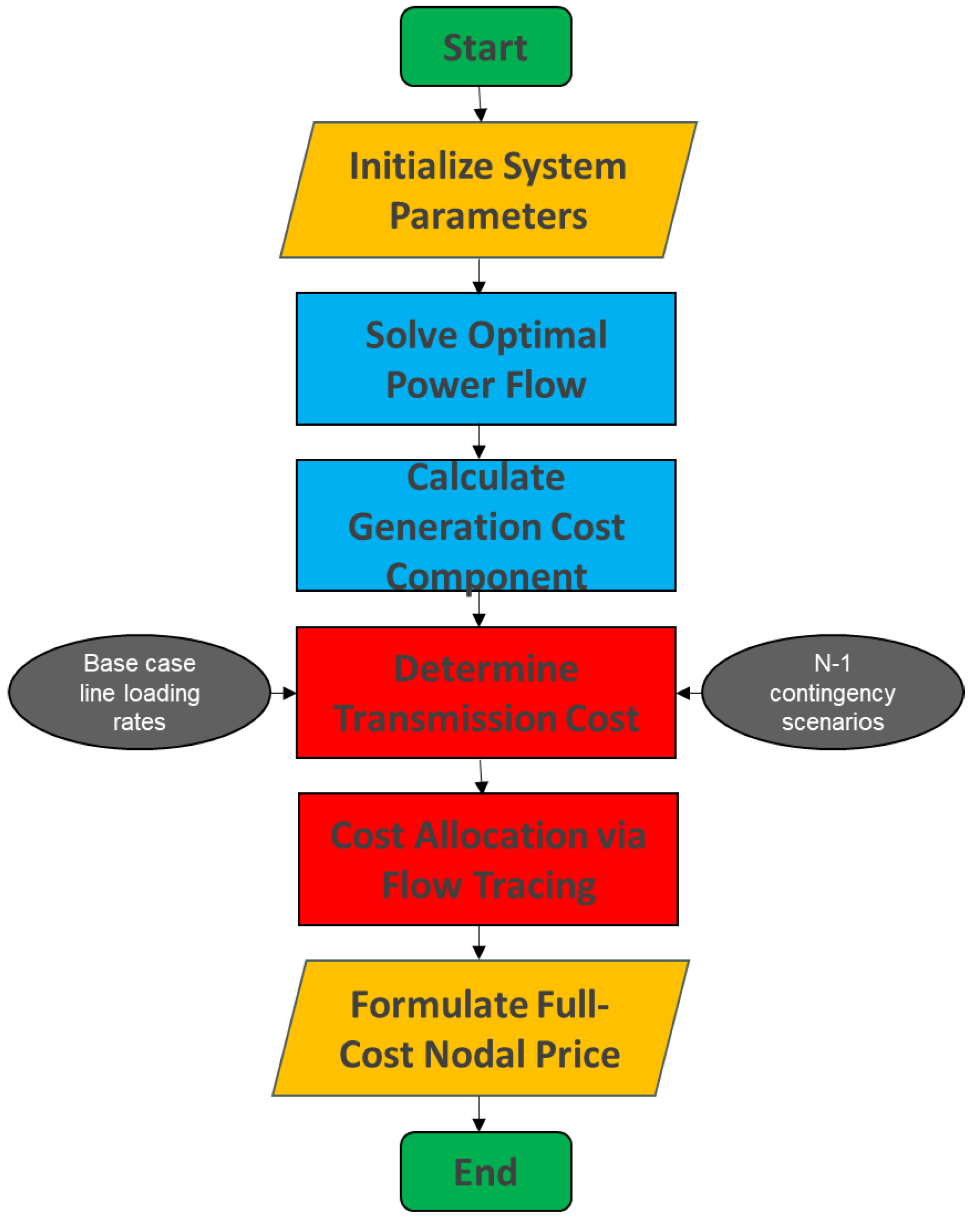
The calculation process for full-cost electricity pricing is illustrated in the following flowchart:
Figure 1.
Full-Cost Electricity Pricing Calculation Flowchart.
3. Case Study
3.1. Case Study on Power Flow Tracing Model
To validate the effectiveness of the proposed full-cost electricity pricing model, this section presents a case study comparing three different pricing schemes. The full-cost electricity price under each scheme is analyzed as follows:
Scheme M1: Nodal marginal price without considering the power flow tracing method.
Scheme M2: Full-cost electricity price without considering the effectiveness of fixed transmission costs.
Scheme M3: Full-cost electricity price incorporating the power flow tracing method.
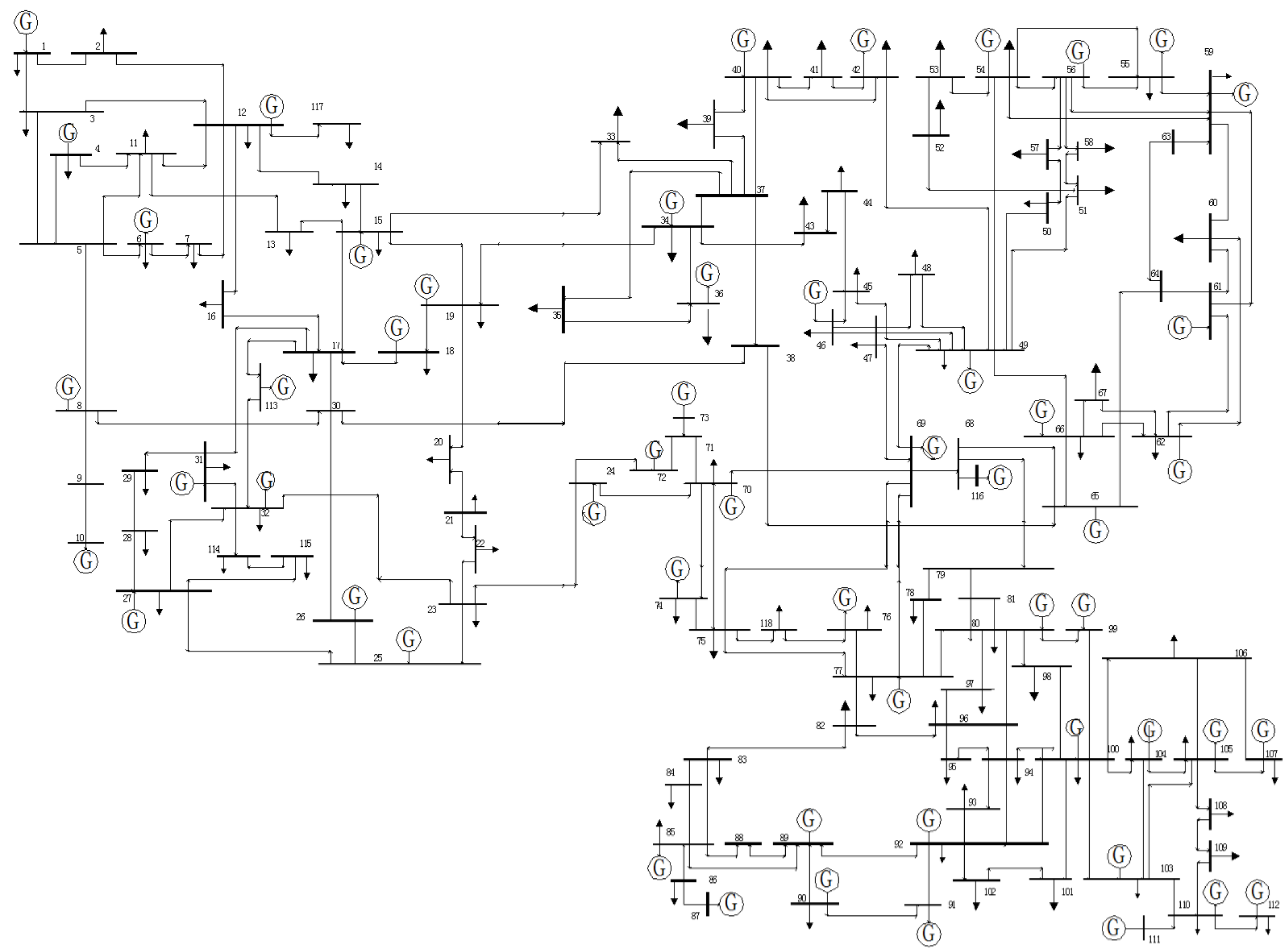
The IEEE 118-bus system is selected as the test system to illustrate the significance of the proposed full-cost pricing model based on power flow tracing. The IEEE 118-bus system consists of 54 generating units and 186 transmission lines, providing a complex network structure and boundary conditions suitable for evaluating the model's performance.
Figure 2.
IEEE 118-Bus System Diagram.
A comparative analysis of nodal electricity prices under the three pricing schemes is conducted.
Figure 3 presents a comparison of full-cost electricity prices in the IEEE 118-bus system under three different schemes. It can be observed that the nodal prices in Scheme M1 remain uniform across all nodes, while in Schemes M2 and M3, the nodal prices at terminal nodes exhibit differentiation. The nodal prices at locations far from generation centers (e.g., Nodes 25, 44, 73, 114) are significantly higher than those near load centers (e.g., Nodes 9, 34, 65, 87). Moreover, at nodes far from generation centers, the full-cost electricity prices in Scheme M3 are significantly lower than those in Scheme M2. Overall, the full-cost electricity prices in Scheme M2 are higher than those in Scheme M3.
The case study results indicate that Scheme M1, based on traditional nodal marginal pricing, does not account for fixed transmission costs. Under the DC power flow model, if no congestion occurs, the marginal price remains uniform across all nodes, failing to capture the variations in electricity consumption across different locations.
Scheme M2 incorporates the full cost of fixed transmission into nodal pricing. The analysis reveals that remote load nodes, due to their greater distance from generation centers, bear the cost of the entire transmission corridor, resulting in significantly higher transmission costs. This full-cost electricity pricing model partially reflects the cost heterogeneity of electricity consumption across nodes by distributing fixed transmission costs accordingly. However, as it does not differentiate between effective and ineffective transmission costs, it fails to account for the actual utilization of each transmission line in the price signals. Consequently, the pricing signals generated are not entirely accurate, leading to an overall higher electricity cost at terminal nodes. This, in turn, may over-incentivize transmission investments, thereby reducing overall investment efficiency.
In contrast, Scheme M3, as proposed in this study, integrates nodal marginal generation costs with effective transmission costs to establish a full-cost electricity pricing framework. The results demonstrate that this pricing approach accurately reflects the extent to which each terminal node utilizes grid resources, thereby capturing the true cost of electricity consumption across different locations and conveying more precise price signals. Under this framework, full-cost electricity pricing aligns with the actual utilization of transmission infrastructure, ensuring that overinvestment is not factored into cost allocation. This effectively mitigates excessive investment incentives for transmission infrastructure, enhances investment efficiency, and ultimately achieves optimal resource allocation. The case study findings validate the superiority of the proposed full-cost electricity pricing model.
3.2. Security-Constrained Power Spot Market Based on Power Flow Tracing Method
Under the concept of full-cost electricity pricing based on power flow tracing, a spot market clearing model is formulated.
3.2.1. Objective Function
The objective function of security-constrained economic dispatch based on full-cost electricity pricing is to minimize total generation costs, as expressed in Equation (13):
where: represents the unit generation cost of the generator at node ; is the generation output at node , is the total number of nodes.
3.2.2. Constraints
1) Generation-Load Balance Constraint
where: is the load demand at node .
2) Generator Output Limits
where: and denote the maximum and minimum output limits of generator , respectively.
3) Transmission Line Flow Limits
where: represents the active power transmission capacity of line .
4) Power Flow and Generation Output Transfer Distribution Factor Constraint
where: represents the generation transfer distribution factor, indicating the sensitivity of power flow on transmission line to the generation output at generator .
5) Full-Cost Electricity Pricing Constraint
Based on the derivation of full-cost electricity pricing, the corresponding constraint is expressed as:
6) Demand Response Function
where: denotes the demand response function at load node , which can be formulated in various forms depending on specific modeling requirements. For the purpose of analytical simplification, this study adopts a linear demand response function, where the adjustment range of demand response is constrained by the upper and lower bounds of the load decision variables [20].
The incorporation of power flow tracing techniques introduces matrix inversion operations and other complex nonlinear expressions, leading to a highly nonlinear model that presents significant computational challenges for direct solution.
To address this issue, an iterative computation approach is proposed in this section. The steps for solving the model are as follows [20]:
1)Set the initial load values and system network boundary conditions.
2)Use a linear programming (LP) solver to compute the economic dispatch.
3)Calculate the marginal generation cost and transmission cost based on the economic dispatch results to obtain the full-cost nodal electricity price. If the convergence condition is met (i.e., the 2-norm difference of the full-cost electricity price vector between two consecutive iterations is below the threshold), proceed to Step 6; otherwise, go to Step 4.
4)The nodal load responds to the full-cost electricity price.
5)Update the initial load values and return to Step 2.
6)Terminate the computation.
The solution process is shown in Figure 4.
3.3. Case Study on Security-Constrained Economic Dispatch in the Power Spot Market
This section evaluates the effectiveness of the proposed security-constrained economic dispatch model based on full-cost electricity pricing through case studies on the IEEE 30-bus system and IEEE 118-bus system.
Since the iterative solution approach is adopted, the demand-side response function can take different functional forms. For simplification, this study assumes a linear demand response function, as given in Equation (3-8):
In the formula: is set to 0.007, and is taken as the initial load value from the IEEE standard system.
This section compares three node pricing and demand response schemes:
Scheme M1: Nodal prices exclude fixed transmission costs, with demand response based on marginal prices. Fixed transmission costs are not differentiated and are allocated to end-users using the postage stamp method after response.
Scheme M2: Nodal prices include fixed transmission costs, with demand response based on full-cost prices. Effective and ineffective transmission costs are differentiated and allocated using the postage stamp method.
Scheme M3 (Proposed): An economic dispatch model incorporating both marginal generation and fixed transmission costs. Demand response is based on full-cost prices, and transmission costs are differentiated and allocated using the power flow tracing method.
The model’s effectiveness is validated through tests on the IEEE 30-bus system and a provincial grid dataset, solved using the CPLEX solver (GAP = 0). Table 1 and Table 2 list the basic parameters for generators and transmission lines in the IEEE 30-bus system, respectively.
Table 1 compares the generation, transmission, and consumption costs under the three schemes:
Generation Cost: Scheme M1, based on nodal marginal pricing without including fixed transmission costs, distorts price signals and limits user response. As a result, generation cost savings are minimal, leading to higher generation costs compared to Schemes M2 and M3.
Transmission Cost: Scheme M1 fails to differentiate between the effectiveness of fixed transmission costs, leading to significantly higher transmission costs than in Schemes M2 and M3. Scheme M3, using power flow tracing, more accurately allocates transmission costs, optimizing flow distribution and further reducing total transmission costs.
Consumption Cost: Scheme M3 results in the lowest total consumption cost, demonstrating that the full-cost pricing economic dispatch model effectively incentivizes user response, thereby reducing consumption costs.
As shown in Table 2, Scheme M3 reduces the total system load by 1.84% compared to Scheme M1 and 0.81% compared to Scheme M2, highlighting the effectiveness of the proposed full-cost electricity pricing model in improving demand-side responsiveness. Figure 6 and Figure 7 illustrate the differences in power flow across the three schemes. Scheme M3 results in an overall reduction in system power flow, driven by more refined price signals. For transmission lines near generation centers (e.g., Lines 1, 6, 8, 9, 24, 26, and 40), the power flow reduction is minimal, and in some cases, it even increases, reflecting a more balanced redistribution of resources. In contrast, transmission lines farther from generation centers (e.g., Lines 7, 15, 16, 18, 36, 37, and 38) show a significant reduction in power flow, indicating the effectiveness of Scheme M3 in alleviating transmission burdens on long-distance corridors. A comparison of Figure 3, Figure 4 and Figure 5 and 3-6 demonstrates that the security-constrained economic dispatch model based on full-cost electricity pricing significantly reduces transmission congestion risks compared to traditional marginal pricing models, while further optimizing power flow allocation relative to the postage stamp method. By rationally allocating fixed transmission costs, the proposed model ensures that full-cost electricity prices reflect the true cost of electricity consumption at each node, incentivizing demand-side adjustments. This results in a redistribution of power flow, shifting transmission burdens from long-distance lines to those closer to generation centers, establishing a "near-high, far-low" power flow pattern that enhances grid efficiency and the economic viability of transmission investments.
Figure 8 shows the load differences between Scheme M3 and Scheme M1, reflecting the impact of the two schemes on load. Scheme M1 does not consider fixed transmission costs, resulting in incomplete price signals and insufficient load response. In contrast, Scheme M3, based on full-cost electricity pricing, encourages greater load-side response to reduce electricity costs, leading to an overall decrease in load. Nodes closer to generation centers (e.g., Nodes 1, 5, 28) show minimal load variation, while nodes farther from generation centers (e.g., Nodes 18, 26, 29) experience significant load reductions due to higher transmission cost allocation. Figure 9 illustrates the load differences between Scheme M3 and Scheme M2. Although Scheme M2 considers fixed transmission costs, the postage stamp method fails to reflect regional differences, leading to higher load reductions at nodes near generation centers. In contrast, distant nodes, with lower cost allocation, show less load response compared to Scheme M3. In conclusion, the load differences highlight that full-cost electricity pricing can accurately reflect the varying electricity costs at different nodes, thereby optimizing load distribution and enhancing load-side responsiveness.
Table 3 lists the nodal electricity prices under the three schemes. Overall, Scheme M1 has the highest electricity prices, followed by Scheme M2, and Scheme M3 has the lowest prices. The main reason is that Scheme M1 incorporates all fixed transmission costs into the electricity prices, while Scheme M2 only includes effective transmission costs. Scheme M3 uses the power flow tracing method to allocate fixed transmission costs, leading to a significant increase in electricity prices at nodes farther from generation centers, reflecting the principle of "costs borne by beneficiaries." At nodes with long supply-demand distances, full-cost electricity prices rise significantly before congestion occurs. Combined with the power flow difference maps, it can be observed that power flow on remote transmission lines decreases, helping to prevent line congestion. Furthermore, the load difference maps in Figure 3, Figure 4, Figure 5, Figure 6 and Figure 7 and 3-8 show that nodes with greater price increases exhibit a more pronounced reduction in load response.
In summary, the proposed method integrates transmission costs into full-cost electricity pricing and considers fixed transmission costs in economic dispatch and demand response, ensuring a more accurate reflection of grid resource utilization. By linking transmission investment returns to actual grid usage, it promotes rational and efficient grid investment.
To further validate its effectiveness, the IEEE 118-bus system with 54 generators and 186 transmission lines is used for analysis.
Table 4 compares generation, transmission, and electricity consumption costs under the three schemes. Scheme M1 has the highest transmission cost, while Scheme M3, better reflecting actual grid utilization, further reduces it. Scheme M1's generation cost is slightly higher due to weaker user response and lower cost savings. Scheme M3 achieves the lowest total electricity cost, highlighting its effectiveness in optimizing demand response.
Figure 10 presents the power flow differences between Scheme M1 and Scheme M3. Overall, Scheme M3 results in slightly lower total power flow. Near-generation lines (e.g., Lines 54, 95, and 97) experience higher flow, while remote lines (e.g., Lines 93, 94, and 126) show significant reductions, indicating a shift of power flow toward generation centers under the proposed dispatch model.
Figure 11 presents the power flow differences between Scheme M2 and Scheme M3. Overall, Scheme M3 results in lower total power flow compared to Scheme M2. Near-generation lines (e.g., Lines 8, 97, and 110) exhibit higher power flow in Scheme M3, while remote lines (e.g., Lines 94, 104, and 127) show significant reductions, further highlighting the effectiveness of the proposed model in redistributing power flow toward generation centers.
Figure 12 compares nodal electricity prices under the three schemes. Scheme M1 has the highest average price, followed by Scheme M2, while Scheme M3 results in lower prices at most nodes. Schemes M1 and M2 yield uniform prices due to the postage stamp method, whereas Scheme M3 increases prices at remote nodes (e.g., Nodes 22, 74, and 92), effectively capturing spatial consumption differences and enhancing demand response incentives.
4. Conclusions
This study applies power flow tracing technology to inter-provincial power market transactions, enabling full-cost allocation based on load utilization. The approach follows the "costs borne by beneficiaries" principle, addressing the omission of fixed transmission costs in traditional nodal pricing.
The method effectively identifies inefficient investments, allocates fixed transmission costs accurately, and incentivizes demand-side adjustments, optimizing grid investment and resource efficiency. By increasing electricity prices at remote nodes, it guides spatial load distribution, reduces long-distance transmission burdens, prevents grid congestion, and enhances long-term resource allocation.
Case studies show that the full-cost pricing-based economic dispatch model effectively implements the "costs borne by beneficiaries" principle. Demand response to new price signals reduces overall power flow, shifts remote line usage toward generation centers, and optimizes load distribution and generation-grid-load interaction. For long-distance supply-demand nodes, higher transmission cost allocation promotes effective demand response, mitigating grid congestion risks and enhancing grid security. By linking transmission investment returns with actual grid utilization, the proposed model supports rational investment decisions, improving economic efficiency and grid sustainability.
5. Patents
Author Contributions
Conceptualization, H.C. and J.Z.; methodology, C.H.; software, S.Z; validation, H.C., J.Z. and G.H.; formal analysis, H.C.; investigation, J.Z; resources, C.H.; data curation, S.Z; writing—original draft preparation, S.Z.; writing—review and editing, C.H.; visualization, S.Z; supervision, J.Z.; project administration, H.C.; funding acquisition, J.Z. All authors have read and agreed to the published version of the manuscript.
Funding
This research was funded by Science and Technology Project of State Grid Corporation of China (5108-202355448A-3-2-ZN)'Research on Inter-provincial Power Spot Trading Mechanism and Key Technologies Adapted to Direct Participation of Large-scale Power Users’.
Conflicts of Interest
The authors declare no conflicts of interest.
Appendix
Appendix 1

Table A1.
Generator Parameters.
| Unit ID | Capacity (MW) | Node Location | Operating Cost ($/MWh) |
|---|---|---|---|
| 1 | 100 | 1 | 380 |
| 2 | 100 | 2 | 400 |
| 3 | 100 | 5 | 370 |
| 4 | 100 | 8 | 390 |
| 5 | 140 | 11 | 350 |
| 6 | 100 | 13 | 360 |
Table A2.
Transmission Line Parameters.
| Line ID | Start-End Node IDs | Transmission Capacity (MW) | Reactance (p. u.) | Investment Cost ($M) |
|---|---|---|---|---|
| 1 | 1-2 | 10 | 0.575 | 61.5 |
| 2 | 1-3 | 10 | 0.165 | 169.2 |
| 3 | 2-4 | 15 | 0.173 | 177.7 |
| 4 | 3-4 | 20 | 0.037 | 41.9 |
| 5 | 2-5 | 5 | 0.198 | 202.3 |
| 6 | 2-6 | 10 | 0.176 | 180.3 |
| 7 | 4-6 | 15 | 0.041 | 45.4 |
| 8 | 5-7 | 10 | 0.116 | 120 |
| 9 | 6-7 | 30 | 0.082 | 86 |
| 10 | 6-8 | 30 | 0.042 | 46 |
| 11 | 6-9 | 80 | 0.205 | 212 |
| 12 | 6-10 | 15 | 0.556 | 560 |
| 13 | 9-11 | 150 | 0.208 | 212 |
| 14 | 9-10 | 80 | 0.110 | 114 |
| 15 | 4-12 | 50 | 0.256 | 260 |
| 16 | 12-13 | 150 | 0.140 | 144 |
| 17 | 12-14 | 20 | 0.256 | 259.9 |
| 18 | 12-15 | 30 | 0.130 | 134.4 |
| 19 | 12-16 | 20 | 0.198 | 202.7 |
| 20 | 14-15 | 10 | 0.199 | 203.7 |
| 21 | 16-17 | 20 | 0.192 | 196.3 |
| 22 | 15-18 | 20 | 0.219 | 222.5 |
| 23 | 18-19 | 10 | 0.129 | 133.2 |
| 24 | 19-20 | 5 | 0.068 | 72 |
| 25 | 10-20 | 10 | 0.209 | 213 |
| 26 | 10-17 | 5 | 0.085 | 88.5 |
| 27 | 10-21 | 30 | 0.075 | 78.9 |
| 28 | 10-22 | 20 | 0.150 | 153.9 |
| 29 | 21-22 | 5 | 0.023 | 27.6 |
| 30 | 15-23 | 20 | 0.202 | 206 |
| 31 | 22-24 | 20 | 0.179 | 183 |
| 32 | 23-24 | 20 | 0.270 | 274 |
| 33 | 24-25 | 20 | 0.330 | 333.2 |
| 34 | 25-26 | 10 | 0.380 | 384 |
| 35 | 25-27 | 10 | 0.209 | 212.7 |
| 36 | 27-28 | 20 | 0.396 | 400 |
| 37 | 27-29 | 10 | 0.415 | 419.3 |
| 38 | 27-30 | 10 | 0.603 | 606.7 |
| 39 | 29-30 | 5 | 0.453 | 457.3 |
| 40 | 8-28 | 5 | 0.200 | 204 |
| 41 | 6-28 | 20 | 0.600 | 63.9 |
References
- Yan, S., Wang, W., Li, X. et al. Research on cross-provincial power trading strategy considering the medium and long-term trading plan. Sci Rep 14, 30137 (2024). [CrossRef]
- 2. SUN Dayan, GUAN Li, HU Chenxu, LUO Zhiqiang, WANG Delin, YU Zhao, CUI Hui, HAN Bin. Design and Exploration of Inter-provincial Power Spot Trading Mechanism[J]. Power System Technology, 2022, 46(2): 421-428. [CrossRef]
- J. Guo, Y. Niu and D. Wang, "Research on new energy direct participation in cross-provincial power trading mechanism," 2023 IEEE 3rd International Conference on Information Technology, Big Data and Artificial Intelligence (ICIBA), Chongqing, China, 2023, pp. 86-90. [CrossRef]
- C. Zhang, Q. Zhao, Y.Ye, Z. Chen, Design and Empirical Research on Cross-provincial and Cross-regional Power Transmission Pricing Mechanism Adapted to Marketized Trading in China, [J]. Procedia Computer Science, 2024, 242, pp. 332-339. [CrossRef]
- Yi Chen, Han Wang, Zheng Yan, Xiaoyuan Xu, Dan Zeng, Bin Ma, A two-phase market clearing framework for inter-provincial electricity trading in Chinese power grids[J]. Sustainable Cities and Society, 2022, 85. [CrossRef]
- GE Rui, CHEN Longxiang, WANG Yiyu, LIU Dunnan. Optimization and Design of Construction Route for Electricity Market in China[J]. Automation of Electric Power Systems, 2017, 41(24): 10-15.
- FAN Yuqi, DING Tao, SUN Yuge, HE Yuankang, WANG Caixia, WANG Yongqing, CHEN Tian'en, LIU Jian. Review and Cogitation for Worldwide Spot Market Development to Promote Renewable Energy Accommodation[J]. Proceedings of the CSEE, 2021, 41(5): 1729-1751. [CrossRef]
- ZOU Peng, CHEN Qixin, XIA Qing, et al. Logical Analysis of Electricity Spot Market Design in Foreign Countries and Enlightenment and Policy Suggestions for China[J]. Automation of Electric Power Systems, 2014, 38(13):18-27. [CrossRef]
- CHEN Qixin, FANG Xichen, GUO Hongye, WANG Xuanyuan, YANG Zhenglin, CAO Rongzhang, XIA Qing. Progress and Key Issues for Construction of Electricity Spot Market[J]. Automation of Electric Power Systems, 2021, 45(6): 3-15.
- CHENG Haihua, ZHENG Yaxian, GEN Jian, WU Han, TANG Honghai, LYU Qiaozhen. Path Optimization Model of Trans-regional and Trans-provincial Electricity Trade Based on Expand Network Flow[J]. Automation of Electric Power Systems, 2016, 40(9): 129-134.
- Alvaro Baillo, Mariano Ventosa, Michel Rivier etal. Optimal Offering Strategies for Generation Companies Operating in Electricity Spot Markets[J] . IEEE Transactions on Power Systems: A Publication of the Power Engineering Society,2004,19(2):745-753.
- Victor Joel E. Franciso. Strategic Bidding and Scheduling in Reserve Co-optimized Based Electricity Spot Markets[C]. TENCON 2010 - 2010 IEEE Region 10 Conference, Japan,2010:592-597.
- Rocio Herranz, Antonio Munoz San Roque, Jose Villar, Optimal Demand-Side Bidding Strategiesin Electricity Spot Markets[J]. IEEE Transactions on Power Systems,2012,27(3):1204-1213.
- F.S. Wen and A.K. David. Optimally coordinated bidding strategies in energy and ancillary service markets[J]. IEE Proceedings - Generation, Transmission and Distribution,2002,149(3):331-339.
- ANG Bin,XIA Ye,XIA Qing,et al. Security constraint economic dispatch of AC/DC interconnected power grid based on Benders decomposition method [J]. Proceedings of the CSEE,2016,36(6) :1588-1595.
- XU Dan,CAI Zhi,ZHOU Jingyang. A fast solution method for large-scale security constraint dispatch based on heuristic linear.
- BAO Minglei, DING Yi, SHAO Changzheng, SONG Yonghua. Review of Nordic Electricity Market and Its Suggestions for China[J]. Proceedings of the CSEE, 2017, 37(17): 4881-4892,5207. [CrossRef]
- BUCHHOLZA W, DIPPLB L, EICHENSEER M. Subsidizing renewables as part of taking leadership in international climate policy: the German case[J]. Energy Policy, 2019, 129: 765-773. [CrossRef]
- S. Dai, Z. Cai, Q. Li and Q. Ding, "Analysis and Design of Inter-provincial Electricity Spot Market Model in China," 2021 IEEE International Conference on Power Electronics, Computer Applications (ICPECA), Shenyang, China, 2021, pp. 355-360. [CrossRef]
- Ali, A., Aslam, S., Keerio, M.U., Mirsaeidi, S., Mugheri, N.H., Ismail, M., Abbas, G., & Othmen, S. Optimal solution of multiobjective stable environmental economic power dispatch problem considering probabilistic wind and solar PV generation. Heliyon 2024, 10(20). [CrossRef]
- Li, Y.; Zeng, Y.; Wang, Z.; Zhao, L.; Wang, Y. Optimal Economic Scheduling Method for Power Systems Based on Whole-System-Cost Electricity Price. Energies 2023, 16, 7944. [CrossRef]
Figure 3.
Comparison of Nodal Electricity Prices in the IEEE 118-Bus System.
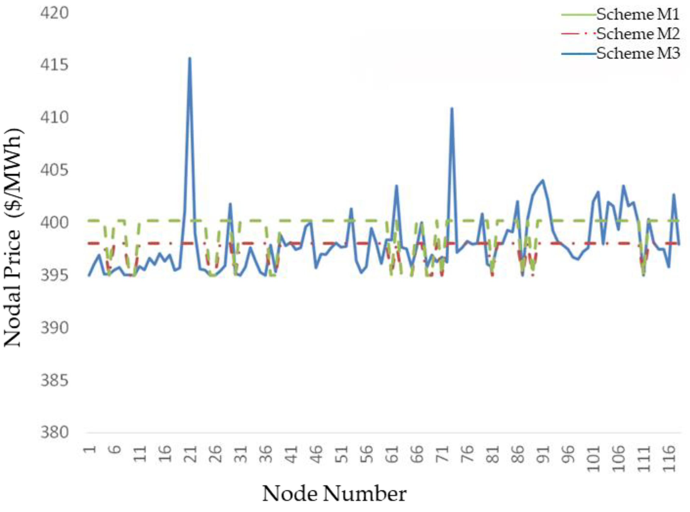
Figure 4.
Algorithm Solution Flowchart.
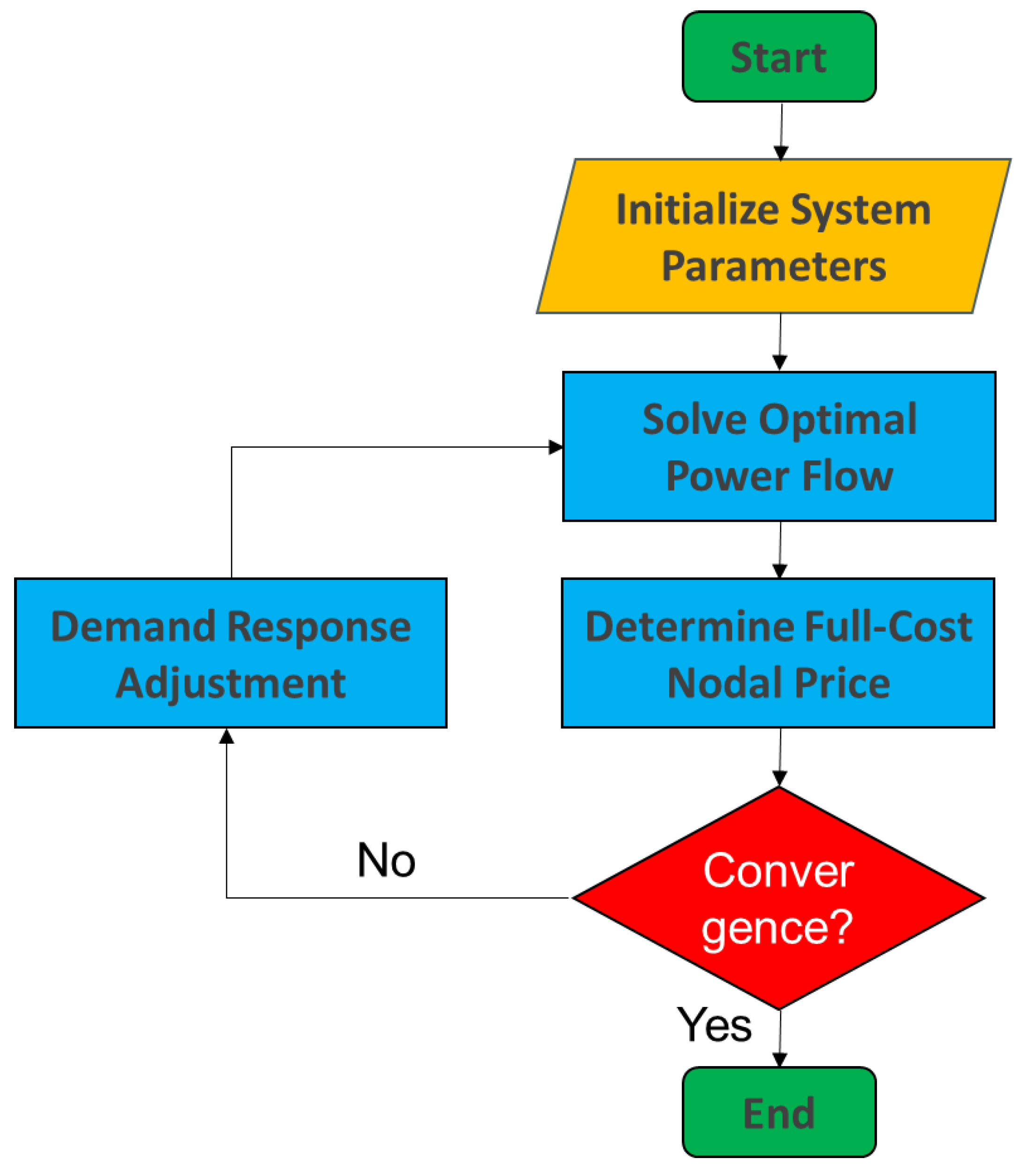
Figure 5.
IEEE 30-bus system network diagram.
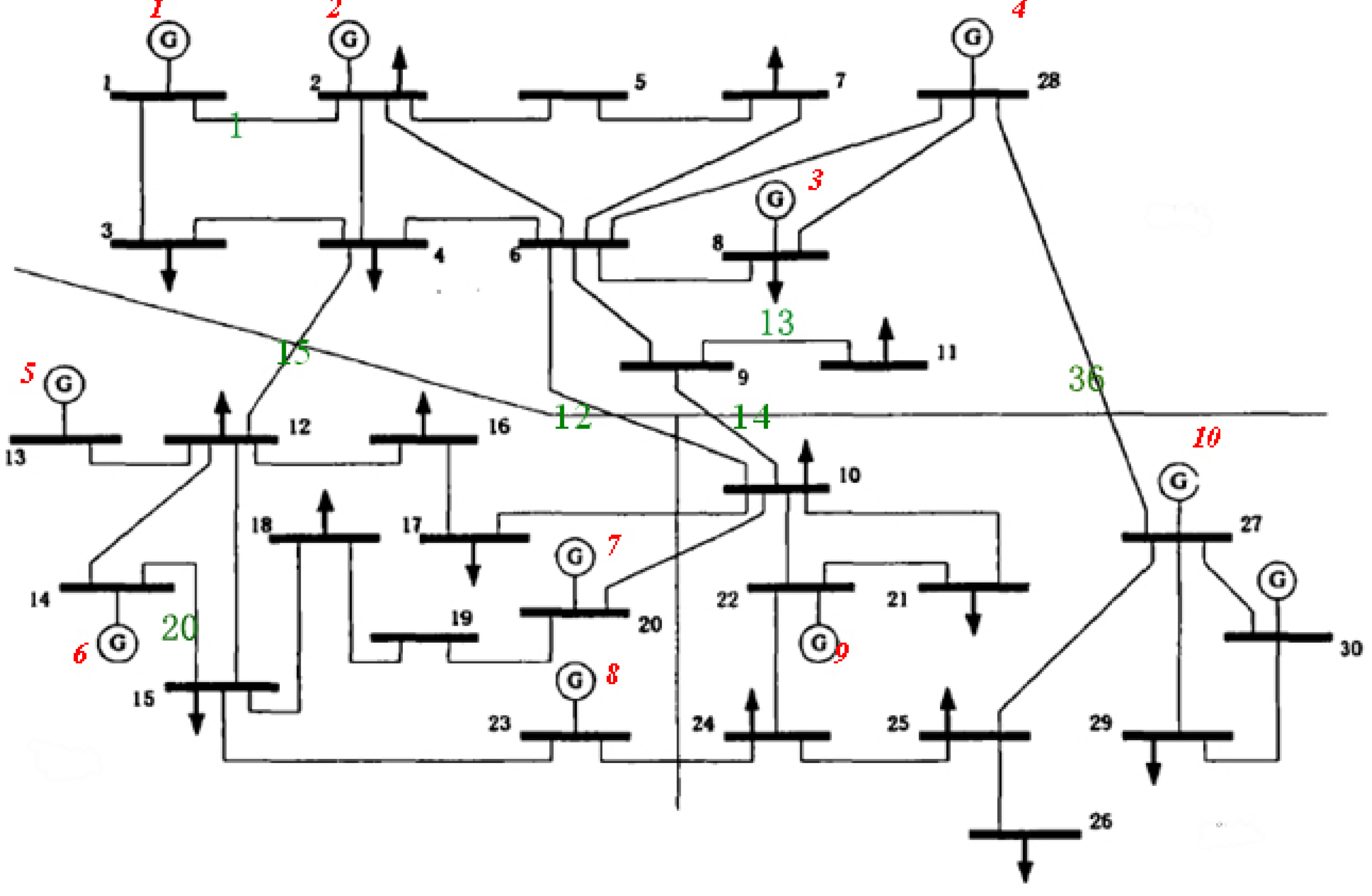
Figure 6.
Power Flow Difference Between Scheme M3 and Scheme M1.
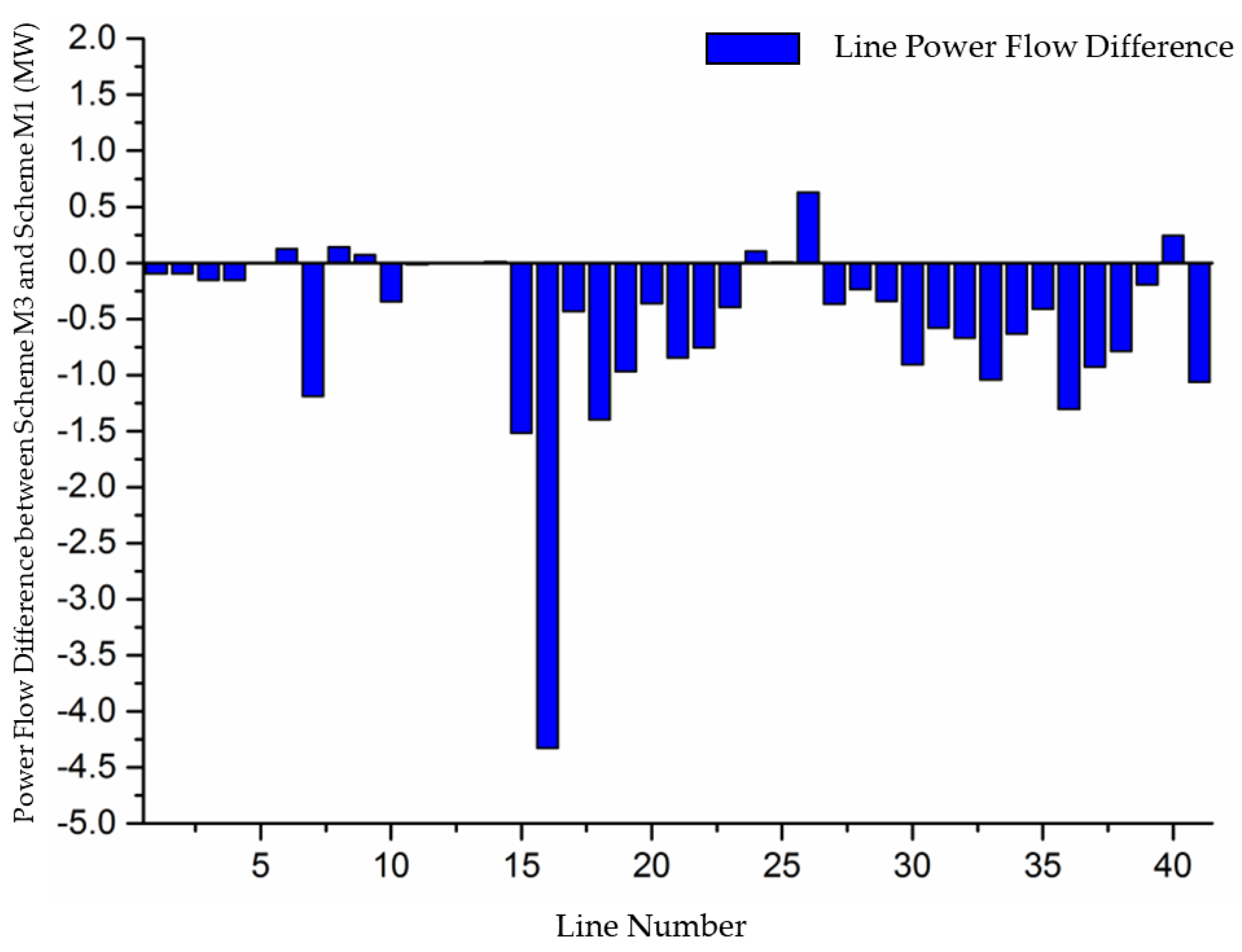
Figure 7.
Power Flow Difference Between Scheme M3 and Scheme M2.
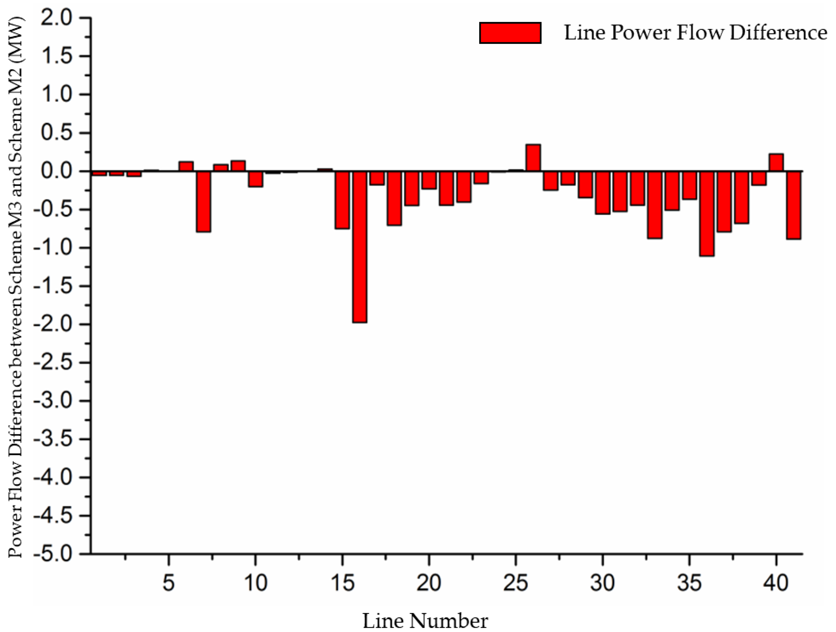
Figure 8.
Load Difference Between Scheme M3 and Scheme M1.
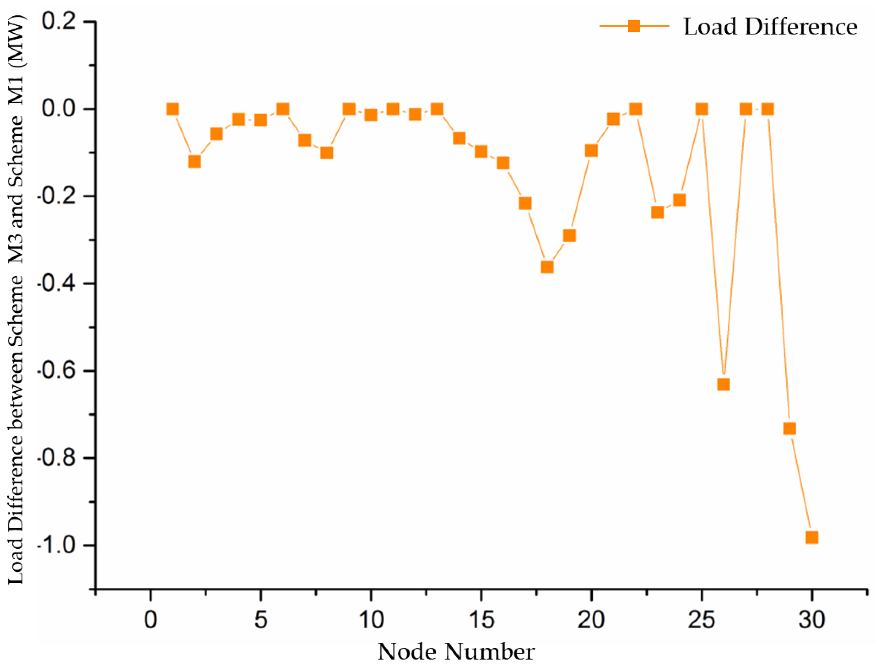
Figure 9.
Load Difference Between Scheme M3 and Scheme M2.
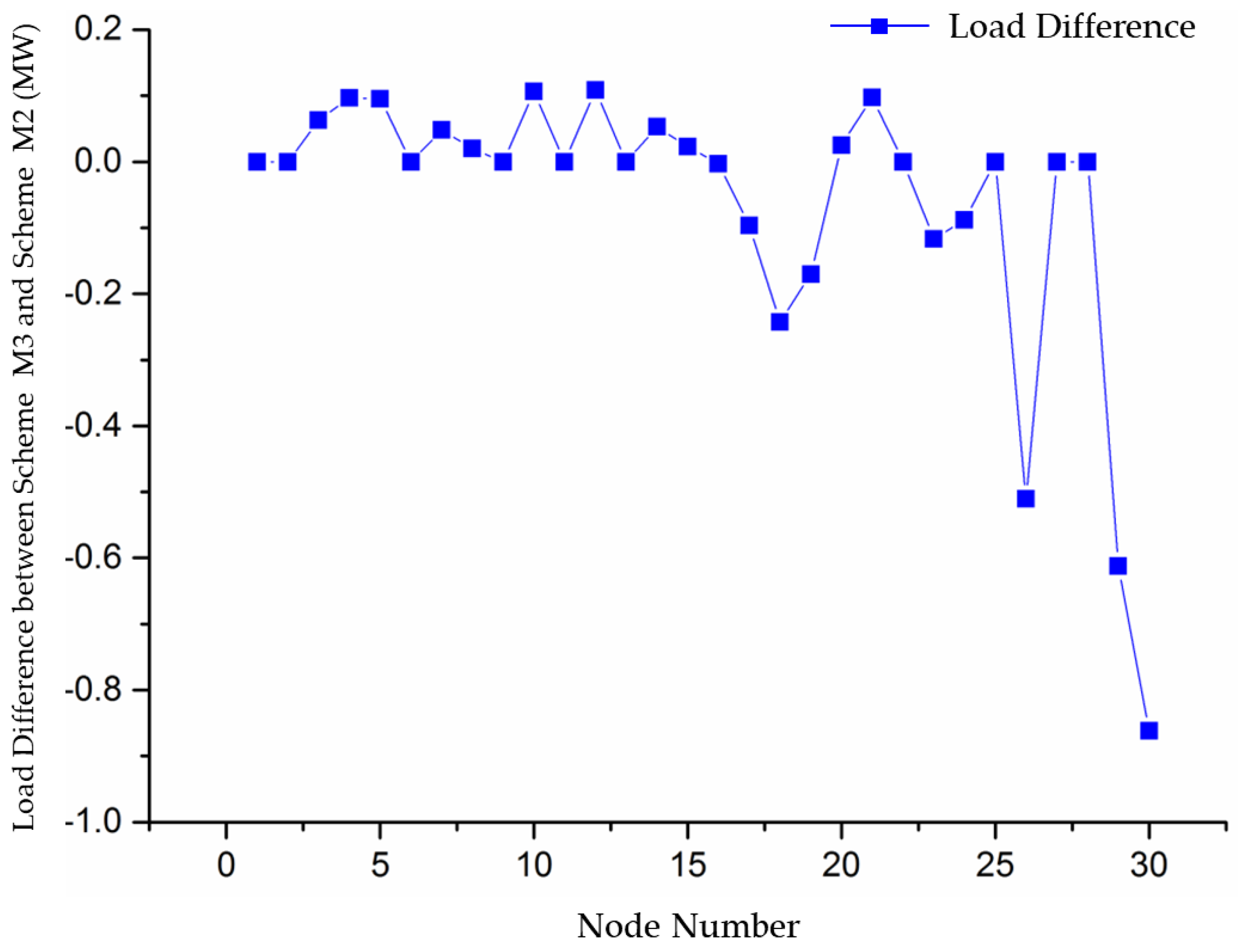
Figure 10.
Difference in Power Flow Between Scheme M3 and Scheme M1.
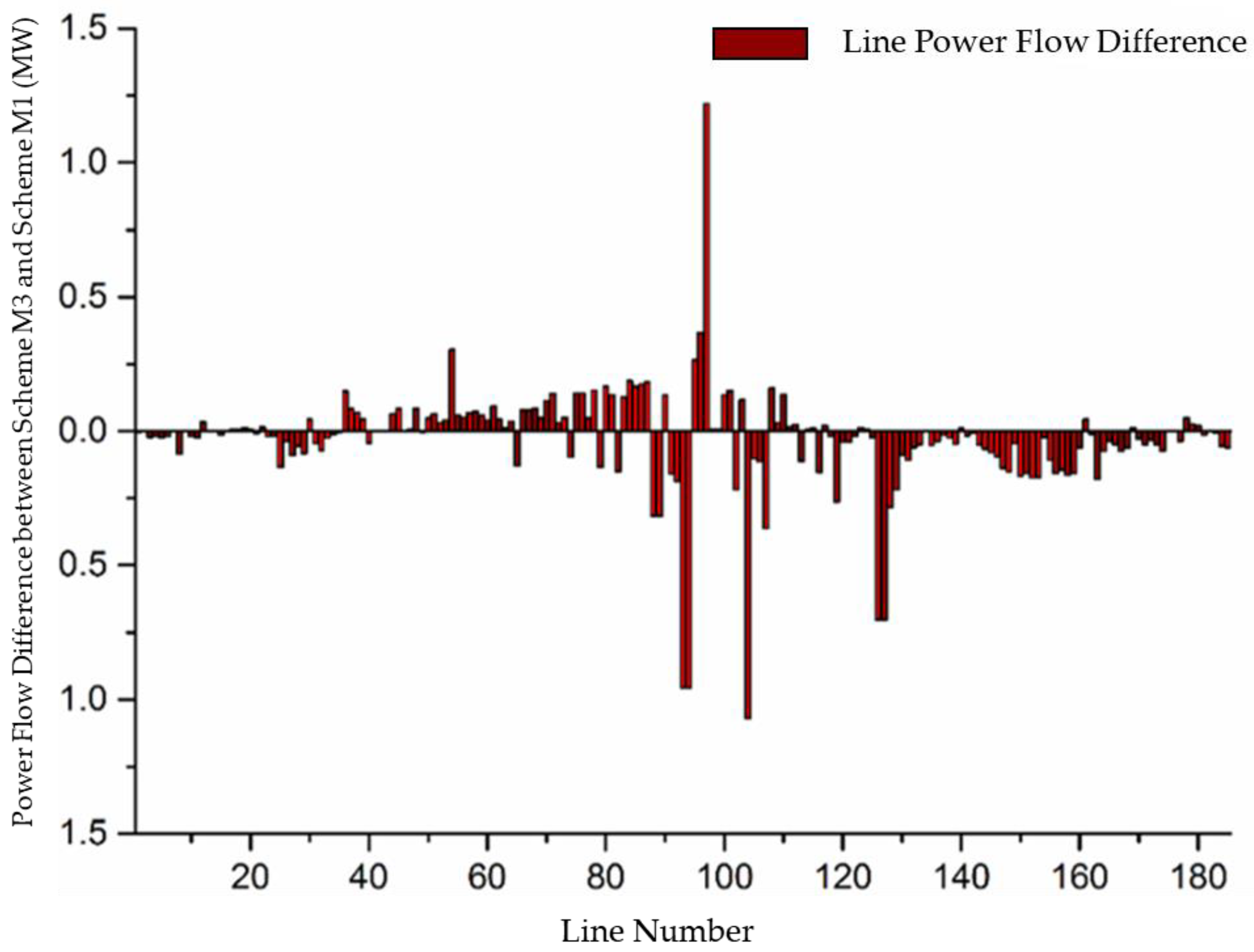
Figure 11.
Difference in Power Flow Between Scheme M3 and Scheme M2.
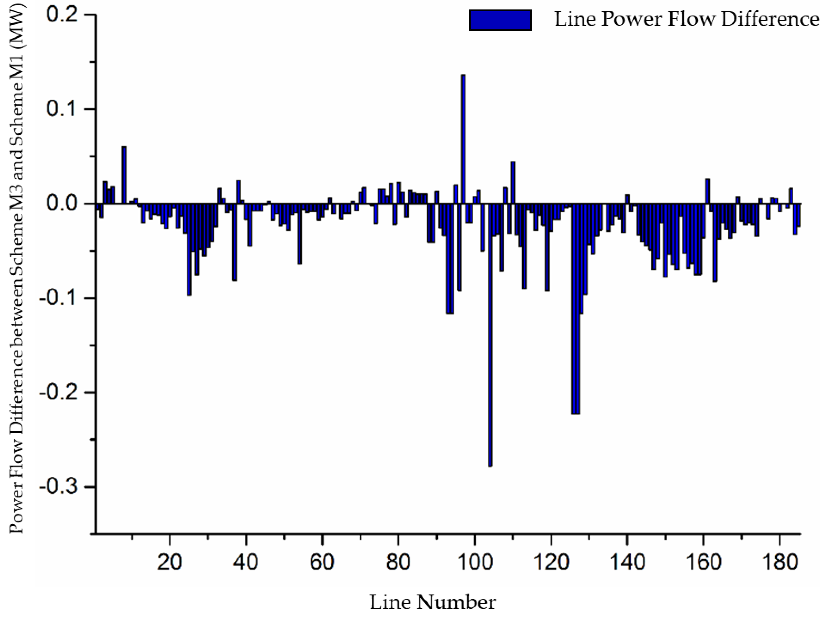
Figure 12.
Comparison of Nodal Electricity Prices Under Three Schemes.
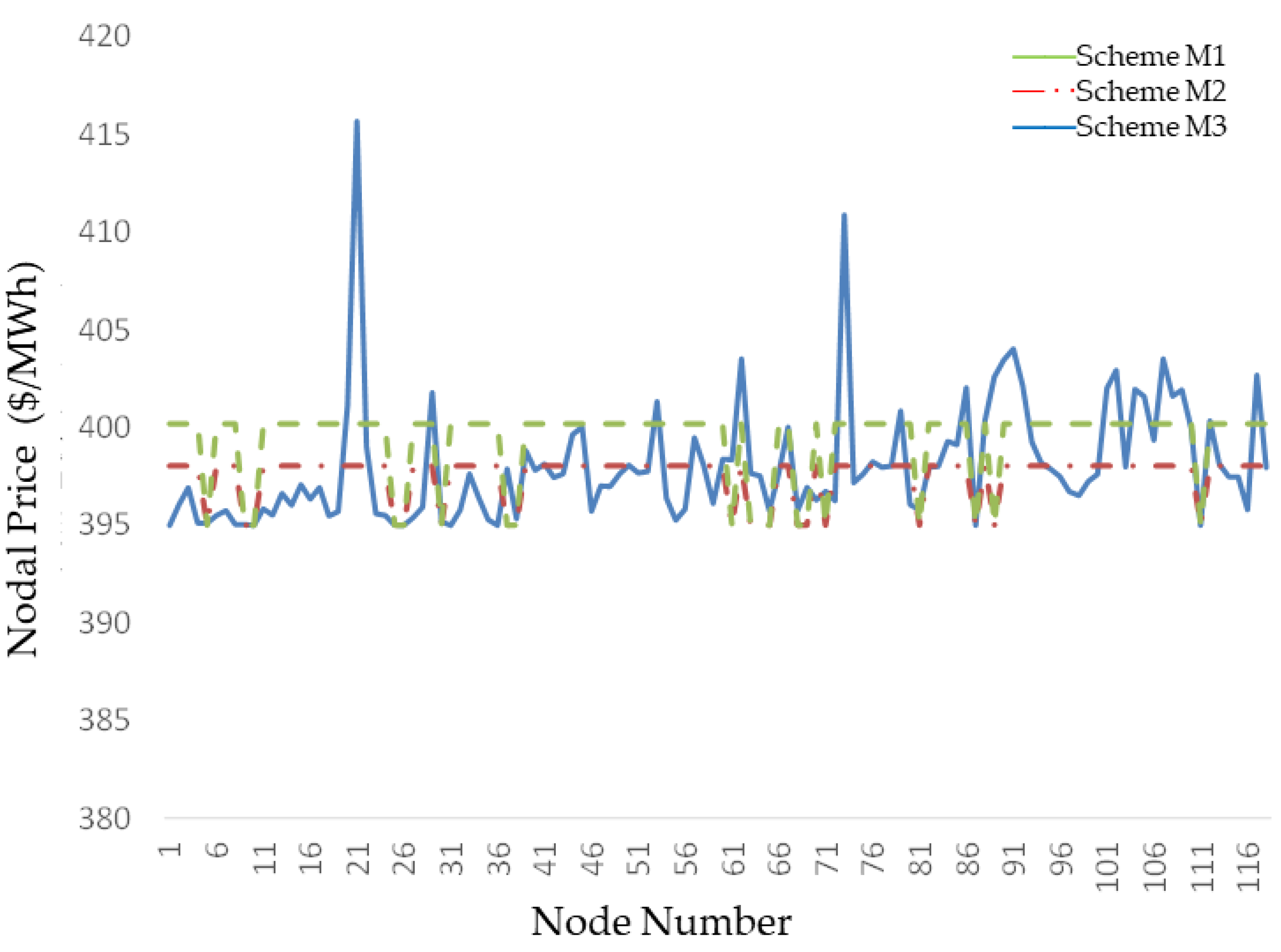
Table 1.
Total cost comparison.
| Scheme | Total Generation Cost ($) | Total Transmission Cost ($) | Total Consumption Cost ($) |
|---|---|---|---|
| M1 | 87799.84 | 8363.00 | 96162.84 |
| M2 | 86888.47 | 4157.00 | 91045.46 |
| M3 | 86180.01 | 3960.53 | 90140.54 |
Table 2.
Total System Load Comparison.
| Scheme | Total Load (MW) |
|---|---|
| M1 | 244.38 |
| M2 | 241.85 |
| M3 | 239.88 |
Table 3.
Comparison of Full-Cost Electricity Prices.
| Node Number | Scheme M1 ($/MWh) | Scheme M2 ($/MWh) | Scheme M3 ($/MWh) | Node Number | Scheme M1 ($/MWh) | Scheme M2 ($/MWh) | Scheme M3 ($/MWh) |
|---|---|---|---|---|---|---|---|
| 1 | 357.48 | 357.48 | 383.79 | 16 | 394.37 | 377.33 | 377.77 |
| 2 | 391.10 | 374.07 | 374.15 | 17 | 394.51 | 377.48 | 391.26 |
| 3 | 393.43 | 376.40 | 367.42 | 18 | 394.41 | 377.37 | 411.99 |
| 4 | 393.83 | 376.80 | 363.03 | 19 | 394.46 | 377.43 | 401.74 |
| 5 | 404.22 | 387.19 | 373.59 | 20 | 394.48 | 377.46 | 373.89 |
| 6 | 360.62 | 360.62 | 369.38 | 21 | 394.57 | 377.54 | 363.63 |
| 7 | 398.73 | 381.70 | 374.80 | 22 | 360.34 | 360.35 | 370.58 |
| 8 | 394.84 | 377.81 | 374.98 | 23 | 394.41 | 377.38 | 394.07 |
| 9 | 360.45 | 360.45 | 360.88 | 24 | 394.54 | 377.50 | 390.14 |
| 10 | 394.58 | 377.54 | 362.37 | 25 | 360.42 | 360.42 | 405.59 |
| 11 | 360.45 | 360.45 | 360.44 | 26 | 394.64 | 377.61 | 450.58 |
| 12 | 394.22 | 377.19 | 361.73 | 27 | 360.49 | 360.49 | 423.21 |
| 13 | 360.00 | 360.00 | 360.00 | 28 | 360.61 | 360.41 | 376.65 |
| 14 | 394.27 | 377.24 | 369.71 | 29 | 394.71 | 377.67 | 465.14 |
| 15 | 394.31 | 377.28 | 374.04 | 30 | 394.71 | 377.67 | 500.79 |
Table 4.
Total cost comparison.
| Scheme | Total Generation Cost ($) | Total Transmission Cost ($) | Total Consumption Cost ($) |
|---|---|---|---|
| M1 | 152885.8 | 20600.7 | 173486.5 |
| M2 | 151803.5 | 13056 | 164859.5 |
| M3 | 151794.6 | 12044 | 163838.6 |
Disclaimer/Publisher’s Note: The statements, opinions and data contained in all publications are solely those of the individual author(s) and contributor(s) and not of MDPI and/or the editor(s). MDPI and/or the editor(s) disclaim responsibility for any injury to people or property resulting from any ideas, methods, instructions or products referred to in the content. |
© 2025 by the authors. Licensee MDPI, Basel, Switzerland. This article is an open access article distributed under the terms and conditions of the Creative Commons Attribution (CC BY) license (http://creativecommons.org/licenses/by/4.0/).
Copyright: This open access article is published under a Creative Commons CC BY 4.0 license, which permit the free download, distribution, and reuse, provided that the author and preprint are cited in any reuse.


