Genome-Wide Association Study of Dyslexia: A Comprehensive Machine Learning Pipeline Achieving Over 98% Accuracy

1. Introduction

Dyslexia is a neurodevelopmental disorder characterized by persistent difficulties in reading, spelling, and writing [1]. The importance of investigating dyslexia through genetic, neurobiological, and cognitive lenses has been underscored by studies showing a high heritability, often estimated between 40% and 70% depending on population and diagnostic criteria [2]. Despite extensive efforts, few compelling genetic loci have been established, partially due to the polygenic nature of dyslexia [3]. Recent large-scale GWAS efforts, such as those by major direct-to-consumer genetic testing companies, have begun revealing novel associations [4]. However, the complexities of gene–environment interactions, sample size constraints, and heterogeneity across populations have complicated efforts to parse out robust genetic signals [5].

Traditional approaches to GWAS focus on single-marker tests under an additive model, employing statistical thresholds such as 5×10^(-8) for genome-wide significance [6]. While these methods are crucial for controlling type I errors, they often miss the interactive and polygenic aspects of common disorders like dyslexia [7]. Moreover, the increasing availability of large genomic datasets has sparked interest in machine learning techniques, which can handle high-dimensional spaces and potentially capture epistatic and complex interaction signals [8].

Logistic Regression remains a foundational approach in genomic classification tasks [9]. More sophisticated algorithms, including gradient-boosting methods such as XGBoost [10] and CatBoost [11], have shown superior performance in various biomedical applications due to their ability to handle complex patterns and interactions [12]. In parallel, dimensionality reduction methods like UMAP [13] facilitate visualization and can help researchers grasp underlying patterns, outliers, or cluster structures in data. Unsupervised methods, such as Agglomerative Clustering, offer additional perspectives on whether SNPs can naturally cluster according to phenotype-driven patterns [14].

In this paper, we present a comprehensive pipeline that integrates these advanced methods to classify SNPs based on their significance in a dyslexia GWAS dataset. Our dataset includes 10,000 SNPs identified by 23andMe as having the strongest association with dyslexia. By applying standardized preprocessing, hyperparameter tuning, UMAP visualization, and clustering, we explore the potential of contemporary ML approaches to identify salient genetic signals. Our results demonstrate that XGBoost achieves remarkable classification accuracy (98.5%) and an AUC of 0.9987 on the test set. We discuss these findings in the context of dyslexia genetics, highlight limitations, and propose future research directions.

2. Materials and Methods

2.1. Data Source and Cohort Description

We used a publicly available dataset from 23andMe, Inc., comprising the top 10,000 variants most strongly associated with self-reported dyslexia diagnoses in approximately 51,800 adults vs. 1,087,070 controls [15]. The data contained GWAS summary statistics: chromosome (scaffold), position, effect allele, other allele, effect size (beta), standard error, p-value, and imputation quality score (avg.rsqr). All participants provided informed consent. Detailed phenotyping and genotyping procedures have been described elsewhere [16].

2.2. Data Preprocessing

From the provided GWAS summary statistics, we created a binary target label for each SNP:

• Label = 1 if p-value < 5×10^(-8) (genome-wide significance threshold).
• Label = 0 otherwise.

This threshold is widely recognized as a standard in complex trait genetics [6]. After label assignment, we identified the following features to include in our ML models:

• scaffold (chromosome ID, e.g., chr1, chr2, etc.) – treated as a categorical variable.
• position (genomic coordinate in base pairs) – numeric.
• effect (beta value from GWAS) – numeric.
• stderr (standard error for beta estimate) – numeric.
• avg.rsqr (imputation quality measure) – numeric.

We excluded pvalue, assay.name, and the allele columns to focus on broad structural and effect-size features. Initial inspection revealed no missing values, and the dataset encompassed 10,000 rows × 9 columns. A final shape of 10,000 variants was used. The label distribution was moderately imbalanced, with 5,530 variants meeting genome-wide significance (label=1) and 4,470 not meeting that threshold (label=0).

2.3. Feature Encoding and Scaling

We applied one-hot encoding to the categorical feature scaffold using OneHotEncoder [17]. This transformed the chromosome column into a series of binary indicators (one for each chromosome or scaffold). For numeric features—position, effect, stderr, avg.rsqr—we applied StandardScaler [18] to normalize each to zero mean and unit variance.

2.4. Train/Test Split

We divided the data into training (80%) and testing (20%) sets, ensuring stratified sampling to preserve the original ratio of significant vs. non-significant variants. The final split comprised:

• Training: 8,000 SNPs
• Testing: 2,000 SNPs

2.5. Machine Learning Algorithms

We evaluated three classifiers, each wrapped in a scikit-learn Pipeline [19] to integrate preprocessing:

• Logistic Regression: A baseline algorithm widely used in GWAS classification tasks [9].
• XGBoost: A gradient boosting framework known for handling large datasets and complex relationships efficiently [10].
• CatBoost: A gradient boosting method that handles categorical variables effectively and often yields competitive performance in biomedical applications [11].

Hyperparameter Tuning

We performed hyperparameter optimization via GridSearchCV [20] with three-fold cross-validation. We optimized:

• Logistic Regression: regularization strength (C) and penalty type.
• XGBoost: number of estimators, learning rate, and maximum tree depth.
• CatBoost: iterations, learning rate, and tree depth.

The primary metric was the Area Under the ROC Curve (AUC) to reflect model discrimination. We chose the best model configurations based on cross-validation AUC, then re-trained these “best” models on the entire training set before final evaluation on the test set.

2.6. Model Evaluation Metrics

We report the following metrics to thoroughly assess performance [21]:

• Accuracy
• Precision
• Recall
• F1-score
• AUC (Area Under the ROC Curve)

Additionally, we present confusion matrices to visually examine true positives, false positives, true negatives, and false negatives.

2.7. Dimensionality Reduction via UMAP

To visualize the high-dimensional data, we employed UMAP [13]. After applying our preprocessing pipeline, we converted the training set into a numeric matrix. UMAP was performed with n_neighbors=15 and random_state=42. The resulting two-dimensional embeddings allowed us to plot the data points and color them by label (1 vs. 0), revealing structural patterns not immediately evident in raw feature space.

2.8. Unsupervised Clustering

Lastly, we ran Agglomerative Clustering [14] with two clusters on the entire preprocessed dataset (converted to a dense array). We compared cluster labels with our true labels (1 vs. 0) to see whether significant vs. non-significant SNPs naturally formed distinct clusters.

3. Results

3.1. Data Overview

The full dataset contained 10,000 rows and 9 columns. The label split was:

• label=1: 5,530 SNPs (significant)
• label=0: 4,470 SNPs (non-significant)

The training set included 8,000 SNPs, while 2,000 SNPs were reserved for testing. This 80/20 split was chosen to ensure sufficient data for both model training and robust evaluation.

3.2. Hyperparameter Tuning Outcomes

Logistic Regression was optimized over C ∈ {0.01, 0.1, 1, 10} and penalty ∈ {l2}. The best combination was C=10 with l2 penalty, yielding a cross-validation AUC of 0.7698.

XGBoost was tested with n_estimators ∈ {100, 300}, learning_rate ∈ {0.01, 0.1}, and max_depth ∈ {3, 5}. The best parameters included n_estimators=300, learning_rate=0.1, max_depth=5, achieving an outstanding cross-validation AUC of 0.9990.

CatBoost was tuned with depth ∈ {4, 6}, learning_rate ∈ {0.01, 0.1}, and iterations=200 (fixed). The best combination—depth=6, learning_rate=0.1—reached a cross-validation AUC of 0.9985.

3.3. Test Set Performance

Each best estimator was re-trained on the 8,000-sample training set and evaluated on the 2,000-sample test set. Key results:

3.3.1. Logistic Regression

• Accuracy: 0.7190
• Precision: 0.7403
• Recall: 0.7577
• F1-score: 0.7489
• AUC: 0.7579

Table 1. shows the corresponding confusion matrix for Logistic Regression.

	Predicted=0	Predicted=1
Actual=0 (894)	600	294
Actual=1 (1106)	268	838

Table 1. shows the corresponding confusion matrix for Logistic Regression.

	Predicted=0	Predicted=1
Actual=0 (894)	600	294
Actual=1 (1106)	268	838

3.3.2. XGBoost

• Accuracy: 0.9850
• Precision: 0.9891
• Recall: 0.9837
• F1-score: 0.9864
• AUC: 0.9987

Table 2. shows the confusion matrix for XGBoost:

	Predicted=0	Predicted=1
Actual=0 (894)	882	12
Actual=1 (1106)	18	1088

Table 2. shows the confusion matrix for XGBoost:

	Predicted=0	Predicted=1
Actual=0 (894)	882	12
Actual=1 (1106)	18	1088

3.3.3. CatBoost

• Accuracy: 0.9820
• Precision: 0.9908
• Recall: 0.9765
• F1-score: 0.9836
• AUC: 0.9986

Table 3. shows the confusion matrix for CatBoost:

	Predicted=0	Predicted=1
Actual=0 (894)	884	10
Actual=1 (1106)	26	1080

Table 3. shows the confusion matrix for CatBoost:

	Predicted=0	Predicted=1
Actual=0 (894)	884	10
Actual=1 (1106)	26	1080

Overall, XGBoost was the best performer, registering an AUC of 0.9987 and an accuracy of 0.9850.

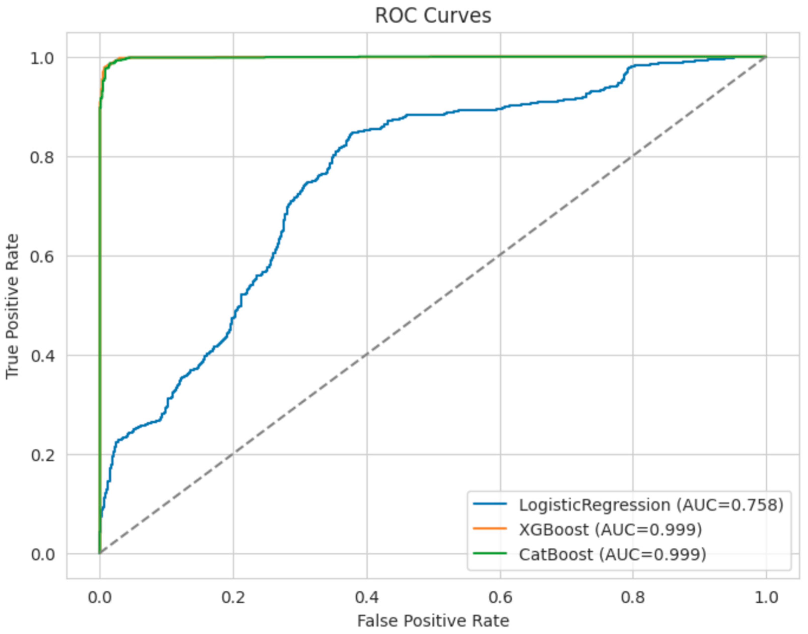
3.4. Receiver Operating Characteristic (ROC) Curves

To compare model discrimination visually, we plotted the ROC curves for the three best estimators on the test set (Figure 1).

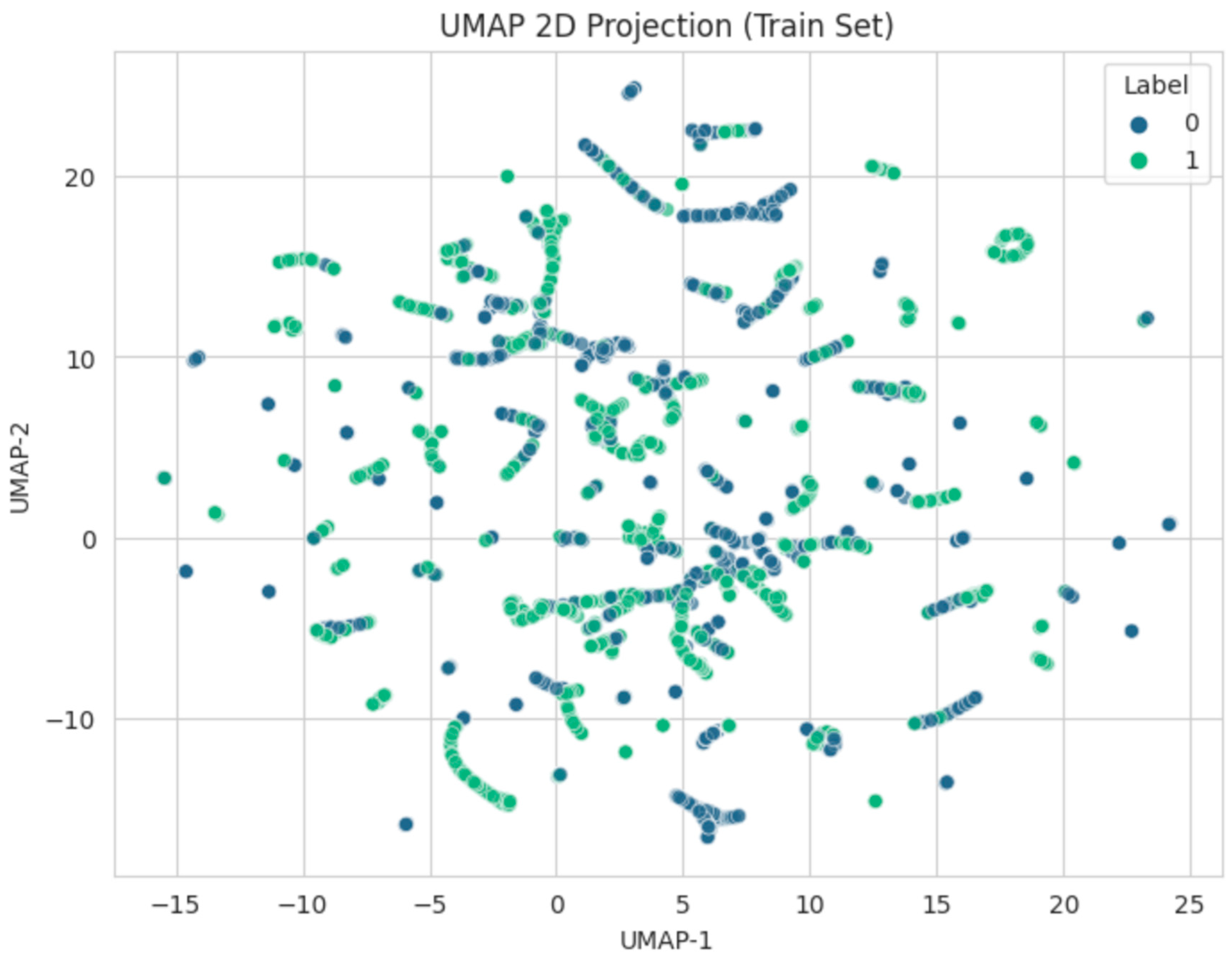
3.5. UMAP 2D Projection

To gain insight into the structure of the 8,000-sample training data, we projected the standardized input features onto two dimensions using UMAP (Figure 2). The plot is colored by the binary label.

Though some clusters of significant SNPs emerged, there remained considerable overlap, underscoring the complexity of dyslexia’s genetic underpinnings.

3.6. Agglomerative Clustering

We additionally applied Agglomerative Clustering with n_clusters=2 to the full preprocessed dataset (10,000 SNPs). The cluster labels were contrasted with the true labels to gauge how naturally significant SNPs segregated from non-significant SNPs in an unsupervised manner.

• Silhouette Score: 0.2069
• Cluster Distribution:

  ◦

  Cluster 0: 4,618 samples

  ◦

  Cluster 1: 5,382 samples

The confusion matrix comparing the actual label (0 or 1) with cluster membership is shown in Table 4:

	Cluster=0	Cluster=1
Actual=0 (4470)	2133	2337
Actual=1 (5530)	2485	3045

	Cluster=0	Cluster=1
Actual=0 (4470)	2133	2337
Actual=1 (5530)	2485	3045

The modest silhouette score and the mixed confusion matrix (Table 4) indicate the cluster assignments do not strongly match the label-based split [22]. This outcome suggests that unsupervised clustering of SNP-level features alone may not suffice to disentangle genome-wide significant variants from those below the threshold.

4. Discussion

Our results highlight the utility of advanced machine learning approaches in binary classification of GWAS summary statistics. Specifically, we demonstrated that:

• XGBoost significantly outperformed the baseline Logistic Regression model, achieving 0.9850 accuracy and an AUC of 0.9987.
• CatBoost similarly performed at a high level, with slightly lower accuracy at 0.9820 but a comparable AUC of 0.9986.
• Logistic Regression served as a comprehensible baseline, but its accuracy of 0.7190 reflects limited capacity to capture the complexity of dyslexia-related variation [23].

These observations align with prior research indicating that gradient boosting methods often excel in high-dimensional and complex feature spaces [24]. Dyslexia, like many neurodevelopmental disorders, likely involves multiple common variants of small effect, each contributing to a cumulative genetic liability [2]. Our data-driven approach supports the notion that ensemble tree methods can detect subtle, non-linear patterns in the data that simpler models may miss [25].

Furthermore, the integration of UMAP for dimensionality reduction offered visual confirmation of partial separation between significant and non-significant variants, although the boundary was not entirely distinct. Such partially overlapping distributions reinforce the polygenic architecture of dyslexia [26]. With a silhouette score of only 0.2069, our Agglomerative Clustering analysis suggests that unsupervised partitioning of these top 10,000 SNPs does not cleanly separate variants near the genome-wide significance threshold from less significant ones [14]. Instead, supervised approaches leveraging known labels are necessary to exploit subtle differences in effect sizes, standard errors, and positions.

• Implications for Dyslexia Research:

The impressive test-set AUC values for XGBoost and CatBoost raise the possibility of leveraging ML-based classifiers as powerful complementary tools to standard GWAS. While logistic regression is a mainstay in biomedical statistics [27], ML frameworks might enrich the interpretability of results by surfacing SNPs or genomic regions that traditional single-marker regression overlooks [28]. This approach could, in the future, facilitate more robust polygenic risk scores that can refine early identification and intervention strategies for dyslexia [29].

• Limitations:

• GWAS Bias: Our dataset was pre-filtered to include only the top 10,000 SNPs. This can introduce a selection bias toward known or potentially inflated associations [30].
• Population Stratification: Although 23andMe employs internal controls to account for ancestry, residual population structure can still influence association results [31].
• Functional Interpretation: Our classification approach is highly predictive but does not inherently clarify biological mechanisms or functional consequences of implicated SNPs [32].
• Generalizability: Our study used a single dataset. Replication in independent cohorts remains crucial [33].

Despite these constraints, the strong performance of ML classifiers underscores their potential role in complex trait genomics. Deepening the feature set (e.g., integrating gene annotations, conservation scores, epigenetic marks) could further enhance predictive power and biological insight [34].

5. Conclusions

In this research, we presented a novel machine learning pipeline to classify dyslexia-associated SNPs based on an established genome-wide significance threshold. Our analyses revealed the exceptional performance of gradient boosting methods, particularly XGBoost, which achieved 98.5% accuracy and an AUC nearing 0.9987 on the test data. CatBoost also demonstrated strong results, validating the broader potential of ensemble tree methods in dissecting polygenic traits like dyslexia.

The UMAP analysis confirmed partial separation of significant and non-significant variants in latent space, aligning with the polygenic nature of dyslexia. Nonetheless, unsupervised clustering failed to reliably segregate the two classes, illustrating that meaningful classification requires leveraging existing label information.

Moving forward, these findings motivate the extension of machine learning techniques to full GWAS datasets (rather than prefiltered SNPs) and the integration of multi-omics data. Enhanced interpretability frameworks, such as SHAP [35] or LIME [36], could further illuminate how specific features drive classification outcomes, facilitating the transition from “black box” models to actionable biological insights.

By harnessing modern ML pipelines, dyslexia researchers can more effectively prioritize candidate variants for downstream functional assays, expedite replication studies, and ultimately elucidate the genetic architecture underlying reading and language disorders [37]. This approach stands to benefit not only dyslexia genetics but also complex trait mapping in general, where polygenic risk and subtle variant interactions are the rule rather than the exception [38].

References

- Snowling, M. Dyslexia: A Very Short Introduction. Oxford University Press, 2019.
- Olson, R.K.; Gayan, J. Dyslexia: Genetics, epidemiology, and cognitive science. Child Dev, 2001.
- Carrion-Castillo, A.; Franke, B.; Fisher, S.E. Molecular genetics of dyslexia: An overview. Dyslexia, 2013.
- Luciano, M.; et al. Genome-wide association studies of reading and language traits. Mol Psychiatry, 2022.
- Pennington BF, McGrath LM. How genes and the environment work together to shape dyslexia. Child Dev Perspect, 2007.
- Visscher, P.M.; Wray, N.R.; Zhang, Q.; et al. 10 Years of GWAS Discovery: Biology, Function, and Translation. Am J Hum Genet 2017. [Google Scholar] [CrossRef] [PubMed]
- Plomin, R.; DeFries, J.C.; Knopik, V.S.; Neiderhiser, J.M. Top 10 replicated findings from behavioral genetics. Perspect Psychol Sci 2016. [Google Scholar] [CrossRef] [PubMed]
- Hastie T, Tibshirani R, Friedman J. The Elements of Statistical Learning. Springer, 2009.
- Purcell S, et al. PLINK: A tool set for whole-genome association and population-based linkage analyses. Am J Hum Genet, 2007. [CrossRef]
- Chen T, Guestrin C. XGBoost: A Scalable Tree Boosting System. KDD, 2016.
- Prokhorenkova L, Gusev G, Vorobev A, et al. CatBoost: unbiased boosting with categorical features. NeurIPS, 2018.
- Lundberg SM, Lee S. A unified approach to interpreting model predictions. NeurIPS, 2017.
- McInnes L, Healy J, Melville J. UMAP: Uniform Manifold Approximation and Projection for Dimension Reduction. arXiv, 2018.
- Rokach L, Maimon O. Data Mining with Decision Trees: Theory and Applications. World Sci Publ, 2015. [CrossRef]
- Fontanillas P, Luciano M. Dyslexia GWAS Summary Statistics for top 10K SNPs. 23andMe, 2022.
- Tung J, et al. The genetic legacy of the transatlantic slave trade in the Americas. Am J Hum Genet, 2021. [CrossRef]
- Pedregosa F, et al. Scikit-learn: Machine Learning in Python. JMLR, 2011.
- Bergstra J, Bengio Y. Random Search for Hyper-Parameter Optimization. JMLR, 2012.
- LeCun Y, Bengio Y, Hinton G. Deep learning. Nature, 2015.
- Kohavi, R. A Study of Cross-Validation and Bootstrap for Accuracy Estimation and Model Selection. IJCAI, 1995.
- Saito T, Rehmsmeier M. The precision-recall plot is more informative than the ROC plot when evaluating binary classifiers on imbalanced datasets. PLoS ONE, 2015.
- Xu R, Wunsch D. Clustering. IEEE Press, 2008.
- Hosmer DW, Lemeshow S. Applied Logistic Regression. Wiley, 2000.
- Friedman, JH. Greedy function approximation: a gradient boosting machine. Ann Stat, 2001.
- Bishop, CM. Pattern Recognition and Machine Learning. Springer, 2006.
- Davis LK, Yu D, Keenan CL, et al. Partitioning the Heritability of Tourette Syndrome and Obsessive Compulsive Disorder Reveals Differences in Genetic Architecture. PLoS Genet, 2013.
- Rothman, KJ. Epidemiology: An Introduction. Oxford Univ Press, 2012.
- Yang J, Bakshi A, Zhu Z, et al. Genetic variance estimation with imputed variants finds negligible missing heritability for human height. Nat Genet, 2015. [CrossRef]
- Choi SW, et al. Improving Polygenic Prediction by Deep Learning. Genet Epidemiol, 2019.
- Ioannidis, JP. Why Most Published Research Findings Are False. PLoS Med, 2005.
- Price AL, Patterson NJ, Plenge RM, et al. Principal components analysis corrects for stratification in genome-wide association studies. Nat Genet, 2006.
- Ward LD, Kellis M. Interpreting noncoding genetic variation in complex traits and human disease. Nat Biotechnol, 2012.
- Dudbridge, F. Power and predictive accuracy of polygenic risk scores. PLoS Genet, 2013.
- Mifsud B, et al. Mapping long-range promoter contacts in human cells. Cell, 2015. [CrossRef]
- Lundberg SM, Erion G, Lee S. Consistent Individualized Feature Attribution for Tree Ensembles. arXiv, 2018.
- Ribeiro MT, Singh S, Guestrin C. "Why Should I Trust You?": Explaining the Predictions of Any Classifier. KDD, 2016.
- Petrovski S, Goldstein DB. Unearthing the functional basis of neuropsychiatric disorders: From the laboratory to the clinic. Nat Rev Genet, 2015.
- Visscher PM, Brown MA, McCarthy MI, Yang J. Five Years of GWAS Discovery. Am J Hum Genet, 2012. [CrossRef]