
Submitted:
20 February 2025
Posted:
21 February 2025
You are already at the latest version
Abstract
The integration of external risk factors (EF) has become increasingly vital for robust credit risk assessment, particularly in emerging economies subject to compounded disruptions. This paper presents a comprehensive, scenario-based methodology for incorporating EF—including pandemic variables (COVID-19 mortality and positive cases), climate anomalies (temperature, road blockages), and social unrest—into machine learning (ML) models. We employ an adapted CRISP-DM workflow, testing stationarity (via Dickey-Fuller), causality (via Granger), and model performance (via AUC and ACC) under scenarios with and without government-backed guarantees. Post-hoc explainability techniques (SHAP, LIME) further reveal which features drive delinquency predictions in EF-enriched contexts. Empirical results, derived from over 8.2 million Peruvian credit records (January 2020–September 2023), confirm that EF integration significantly improves predictive accuracy. Time-lagged mortality (COVID MOV) emerges as the strongest single predictor, while combined crises (pandemic, climate, social unrest) amplify delinquency risk. Models such as XGB, CNN, and XNN exhibit the highest adaptability, consistently attaining statistical significance across different partitions of economic activities. Beyond enhancing model accuracy, EF inclusion highlights key drivers—borrower income stability, debt management, EF severity—thereby supporting more transparent, proactive strategies for financial institutions aiming to mitigate credit defaults in volatile, multi-factor environments.
Keywords:
loan
; credit risk
; prediction
; machine learning
; external factors
1. Introduction
Currently, artificial intelligence (AI), machine learning (ML), and process digitization are fundamental elements of daily life. This trend began in the 1990s with the global expansion of the Internet [1] and notably intensified during the COVID-19 pandemic [2]. Simultaneously, the increase in the use of online credit has generated large volumes of data [3], leading the financial industry to the imperative need to develop advanced technological tools for risk prediction and effective uncertainty management [4], that include exogenous variables in the process [5,6]. Presently, scoring models and machine learning techniques are common for risk prediction, applying innovations based on exhaustive data analysis, Data-Driven Innovation (DDI) [7], and the BIG DATA concept [8,9].
In the context of rising demand, credit risk levels show a significant increase [10,11]. Despite the growing integration of Data-Driven Insights (DDI) and ML in the financial sector, substantial challenges persist, leaving numerous applications unexplored [12,13,14,15]. The application of ML techniques during unpredictable events, such as the 2008 housing crisis [2,16], the COVID-19 pandemic [17], and the impacts of climate change [18], have exposed critical limitations in risk assessment methodologies and revealed considerable uncertainties in their outputs [2,19,20,21]. These challenges underscore the need to examine the influence of external factors (EF) on the accuracy and robustness of ML models in credit risk evaluation [7,22], particularly concerning the inclusion of sequential or time-series data, which are commonly encountered in credit risk scenarios [23]. Moreover, these issues emphasize the need to ensure explainability in ML-driven predictions [24], both to facilitate informed decision-making by stakeholders and to maintain transparency for all parties involved [25].
The main objective of this article is to address the integration of variables sensitive to external risk factors into machine learning models for credit risk assessment, a critical yet insufficiently explored topic in the academic context. Peru, as a case study, represents a particularly relevant scenario: it was the country with the highest COVID-19 death rate per 100,000 inhabitants during the pandemic [26], it faced the periodic and devastating effects of the El Niño phenomenon [18], and it experienced intense social unrest following the attempted coup in December 2022 [27]. These events have directly impacted the microcredit market by targeting small businesses, a sector highly vulnerable to risk volatility [18].
Although related economic analyses exist, a significant gap persists in academic research on the impact of EF on credit risk assessment, particularly within the Peruvian context. This study aims to address this gap by, offering valuable insights into its potential applicability and extrapolation to other emerging economies [18]. To this end, EF-related variables are integrated into credit risk models through causality and stationarity tests [28]. These variables are derived from public time series data and combined with proprietary data from a financial institution, referred to in this study as the ’financial model’ (FMOD). This innovative strategy not only enhances the predictive power of ML models but also establishes a replicable methodology for integrating diverse EF indicators into future risk prediction studies.
The FMOD dataset plays a pivotal role in this study. It incorporates a unique variable that identifies loans supported by government intervention during periods influenced by EF, such as climate change, social unrest, and the COVID-19 pandemic. This variable allows for the detection and detailed analysis of the potential biases introduced by mitigation programs designed to address economic disruptions. By explicitly accounting for these interventions, the FMOD dataset provides a nuanced understanding of how state-led programs shape credit risk dynamics and borrower behavior under varying external conditions.
Moreover, the FMOD dataset includes monthly updated records of delinquency days, enabling granular analysis across distinct periods. This temporal precision facilitates an in-depth exploration of the interplay between EF and default patterns, thus enhancing the methodological rigor of credit risk assessment. By integrating time-series data with real-world financial indicators, the FMOD dataset offers a robust and replicable framework for evaluating the influence of EF and government programs on financial stability and credit behavior in emerging markets.
Finally, this study evaluated the impact of EF on the predictive accuracy and explainability of ML models. Particular attention is paid to identifying the most influential factors when incorporating external variables into predictive frameworks. By addressing these challenges, this research not only fills a critical gap in the existing literature but also advances the understanding of EF’s effects on credit risk in emerging economies. This contributes actionable insights for policymakers and financial institutions aiming to enhance resilience in volatile economic environments.
2. Related WORK
This article aligns its focus with the research questions outlined in Table 1, centering on the interplay between external factors and credit risk assessment. Particular emphasis is placed on the importance of explainability in ML-driven models, as understanding how EF impacts credit risk is critical for decision-making and actionable insights.
Credit risk, an inherent component of financial activities, emerges when there is delinquency in fulfilling credit obligations, because of the inability or lack of intention to pay [29]. This study, focuses on the former, as it is strongly influenced by demographic variables such as economic activity and household income [29], which can be significantly affected by external factors [11]. Ensuring the explainability of these relationships is critical for building trust and providing actionable insights for policymakers, financial institutions, and affected stakeholders.
The external factors considered in this study include:
- COVID-19 Pandemic: This global crisis posed an unprecedented challenge to financial stability, leading to increased credit risk and non-compliance with financial obligations [30]. Its economic impacts, propagated through supply chains, disrupted payment systems and affected household finances [31,32].
- Climatic Factors: Climate-related events such as droughts, floods, and landslides introduce significant risks to financial stability, increasing default rates and credit risk [18]. Additionally, extreme weather events increase the cost of essential goods, forcing households to prioritize basic needs over loan repayments.
To explore these relationships, a study focusing on Peru from January 2020 to September 2023 was conducted. The analysis was based on a comprehensive dataset comprising over 8.2 million records, as summarized in Table 2. This dataset integrates diverse EF, such as COVID-19 positive cases and deaths, road blockages, and temperature anomalies, along with financial delinquency and credit activity data, ensuring a multifaceted approach to understanding credit risk dynamics under external influences.
The datasets were selected based on their ability to capture the intensity and variability of EF during the study period. Figure 1 illustrates normalized time series, providing a uniform representation of the external events.
Figure 1 illustrates the trends of various external factors, including COVID-19 cases (positive and dead), social unrest, road blockages due to social unrest and weather, and temperature anomalies. Peaks in certain factors, such as COVID-19 cases and social unrest, were clearly visible during specific periods, indicating their significant occurrence and potential impact on other events or systems.
The analysis prioritizes the explainability of the results, ensuring that insights derived from machine learning models are interpretable and actionable. By integrating datasets on COVID-19 cases and deaths, climatic factors such as temperature anomalies and road blockages, and social unrest metrics, this study aimed to understand how EF influences delinquency behavior and credit risk.
This approach not only evaluates the predictive accuracy of machine learning models but also examines their capacity to provide transparent explanations for the relationships uncovered, ensuring their practical relevance for decision-making in volatile and complex environments.
3. The Proposed Model
To evaluate the influence of EF on credit risk, we propose an adapted version of the Cross-Industry Standard Process for Data Mining (CRISP-DM). This approach was designed to systematically incorporate EF into ML workflows, ensuring both practical applicability and theoretical rigor, as illustrated in Figure 2. This model has been successfully applied in previous studies to analyze EF during crises [34,35].
Figure 2 illustrates a modified CRISP-DM (Cross-Industry Standard Process for Data Mining) framework tailored for analyzing external factors (EF). It outlines the sequential steps, including dataset analysis, feature representation, data preparation (with normalization standardization), testing with and without external factors, selecting predictive models, and applying explainable AI (XAI) tools such as SHAP and LIME for feature explanation.
3.1. Workflow Description
- 1.
- Dataset Definition and Feature Selection: The process begins by determining the relevant datasets and conducting a comprehensive analysis of the phenomena to be evaluated (EF in this study). Feature selection was guided by established methodologies [36], identifying attributes with high relevance to credit risk prediction, including both internal (e.g., loan characteristics) and external (e.g., EF) variables. The selected features were refined using feature importance techniques, such as Recursive Feature Elimination (RFE) and Mutual Information (MI), ensuring that only the most significant predictors were retained.
- 2.
- Data Preparation: Preprocessing involved standardizing and normalizing the dataset (using sum normalization) to homogenize the data scales. Additionally, missing data were handled using multiple imputation techniques to maintain dataset integrity [36].
- 3.
-
Integration of External Factors: To evaluate the impact of EF on credit risk prediction, additional variables corresponding to EF (e.g., COVID-19, temperature anomalies, social unrest) were incorporated into the dataset. These variables were derived from time-series analyses and causal relationships, validated through statistical methods such as the Dickey-Fuller test and the Granger causality test [37].The Dickey-Fuller test was employed to verify the stationarity of the time series data, ensuring that relationships between variables were not spurious and that the models yielded reliable results [37]. The stationarity of time series is critical, particularly when external factors such as COVID-19 cases, mortality rates, and roadblocks caused by weather events influence the temporal dynamics. The test is described mathematically as:where:
- : First difference in time series ().
- : A constant.
- : A trend term.
- : Lagged value of the time series.
- : Coefficients of lagged differences.
- : The error term.
- p: The number of lags.
Following the confirmation of stationarity, the Granger causality test was applied to evaluate the causal influence of these external factors on economic activities. The test, widely used in econometric studies, is defined as:where:- : Lagged values of series .
- , , and : The coefficients.
- : The error term.
Lag variables were calculated to capture delayed effects, with lag periods tailored to each EF (e.g., quarterly for temperature anomalies, monthly for social unrest and COVID-19). These statistical methods ensured rigorous validation of the causal relationship between EF and economic activities that influence credit defaults. - 4.
- ML Model Training and Hyperparameter Tuning: Advanced ML models (e.g., CNN, XGB, XNN, and EBM) were trained on datasets both with and without EF to assess their predictive contributions. Hyperparameter tuning was conducted using grid search and Bayesian optimization to enhance the model performance. To address the class imbalance in the dataset, techniques such as Synthetic Minority Oversampling Technique (SMOTE) [38] and class-weighted loss functions were employed [39,40].
- 5.
- Evaluation and Explainability (XAI): Models were evaluated using metrics such as Accuracy (ACC) and Area Under the Curve (AUC) across multiple folds (10-fold cross-validation). To enhance interpretability, post-hoc explainability techniques such as SHapley Additive Explanations (SHAP) and Local Interpretable Model-Agnostic Explanations (LIME) were applied [41] . These methods highlight the most influential features in predicting credit delinquency both before and after incorporating EF [25].
- 6.
- Comparison of Scenarios: The workflow was executed in parallel for scenarios excluding EF and those incorporating EF. This allowed for a direct comparison of the model performance and the added value of EF inclusion.
3.2. Key Enhancements in the Current Study
- The integration of explainability methods (SHAP and LIME) provides actionable insights for decision-makers in financial institutions.
- Comprehensive feature selection processes ensuring only the most predictive attributes were retained.
- Rigorous hyperparameter optimization to maximize model performance and robustness.
By employing this adapted CRISP-DM workflow, this study contributes a systematic and replicable methodology for evaluating EF in credit risk contexts, particularly during crises.
Figure 3 depicts the impact of COVID-19 on economic activities by comparing delinquency rates with the economic impacts over time. The graph highlights fluctuations in economic impact trends, particularly during pandemic peaks, and distinguishes patterns between financial and personal impacts (F+P) and movement-related impacts (CR Impact F+Mov).
Figure 4 illustrates the impact of social unrest and climatic factors on economic activity from December 2022 to September 2023. It compares delinquency rates with the economic impact of social unrest, weather, and temperature anomalies, and shows significant spikes during periods of intensified external disruptions.
4. Research Strategy
The evaluation period for this study was defined based on the behavior of the monthly classification variables, starting from the onset of the impact of EF until stabilization, as shown in Figure 3 and Figure 4. Stabilization was defined as the point at which the slope of the curve representing the proportion of bad payers (red line) began to level off.
Evaluation Periods
-
COVID-19: The evaluation period spans March 2020 to January 2022. Loans disbursed until October 2021 were included to account for a 60-day grace period before delinquencies appeared, ensuring unbiased results (Figure 3).During the analysis of the COVID-19 external factors, it was identified that the trends in the number of positive cases and deaths often showed opposing behaviors. To address this, an additional experiment was conducted in which the death curve was shifted from one period to the right, referred to as the COVID MOV. This adjustment considered the estimated incubation period of the disease and the time to potential fatality, typically ranging from 2 to 3 weeks. By aligning the death data with this temporal delay, this analysis aimed to capture the causal relationship between disease progression and its impact on credit delinquency rates. This methodological adjustment is illustrated in Figure 3 (green dotted line).
- Social Unrest and Climate Factors: Data from December 2022 to September 2023 were analyzed, with loans disbursed up to June 2023 considered under the same grace period logic (Figure 4).
Data Preprocessing
- Data normalization and standardization were applied to homogenize scales [42].
- Features with correlations above 90% were removed to prevent redundancy.
- SMOTE was used to balance the dataset [43].
Machine Learning Models We implemented the following models to evaluate the binary classification tasks, prioritizing interpretability and predictive performance:
- Traditional Models: Linear Discriminant Analysis (LDA), Quadratic Discriminant Analysis (QDA), and k-Nearest Neighbors (kNN) [43].
-
Explainable Models:
-
Feedforward Neural Networks: Variants of Feedforward Neural Networks (FFNN) were explored:
- -
- Standard Feedforward Neural Network (FFN): A classical architecture used as a baseline for comparison.
- -
- Feedforward Neural Network with Sparse Regularization (FFNSP): Incorporates sparsity constraints to enhance generalization and reduce overfitting [47].
- -
- Feedforward Neural Network with Local Penalty Regularization (FFNLP): Local penalty terms are applied to balance feature contributions and improve interpretability [48].
- Deep Learning: Convolutional Neural Networks (CNN), included for their ability to capture complex relationships in both spatial and temporal data [49].
Each model was trained and validated using a 10-fold cross-validation split (60% training, 20% validation, 20% testing) [50]. Hyperparameter tuning was conducted using grid search and Bayesian optimization to ensure optimal performance across all configurations.
Explainability with XAI To address concerns about interpretability, SHAP and LIME were applied to identify the most influential features in predicting credit delinquency both before and after incorporating EF. Models such as XNN and EBM provided native interpretability, complementing these post-hoc methods.
Statistical Evaluation The impact of EF on model performance was assessed using Student’s t-test (Equation 3), applied to metrics such as ACC and Area AUC from the cross-validation folds, with a significance level of [51].
where:
- : Mean of metrics from ten folds.
- : Hypothetical mean under the null scenario.
- s: Standard deviation of metrics.
- n: Number of folds ().
Economic Activity Relevance
The dataset, comprising 367,000 loans (see Table 2), was analyzed based on its concentration across economic activities. This analysis is particularly relevant, as the impact of EF on these activities amplifies exposure to credit risk. The distribution of loans is as follows:
- 80% Concentration: 80% of the loans are concentrated in 78 economic activities.
- 99% Concentration: 99% of the loans are concentrated in 326 economic activities.
- 100% Concentration: 100% of the loans are distributed across 660 economic activities.
Figure 5 illustrates these groupings, highlighting the increased dispersion and noise as the number of activities increases. To ensure a comprehensive analysis, the results were further examined by including and excluding loans affected by government-backed programs, thereby isolating the potential biases introduced by such interventions.
Research Limitations and Biases
While this study provides valuable insights into the influence of EF on credit delinquency predictions, several limitations and potential biases must be considered:
- Context-Specific Findings: The analysis is based on data from the Peruvian context, which may limit the generalizability to other regions with different economic, social, and environmental dynamics. Future research should incorporate external validation by using datasets from diverse geographical areas to evaluate the transferability of the proposed methodology.
- Training Data Bias: Dataset imbalances and underreporting of delinquency during government interventions may introduce biases. Although SMOTE has been used to address class imbalances, residual biases related to data collection practices or policy impacts may persist.
- Model Transparency: While explainability techniques such as SHAP, LIME, and interpretable models (e.g., XNN, EBM) have been employed, the use of black-box models like CNN and XGB remains a challenge. This lack of inherent transparency could hinder their applicability to financial institutions, where explainability is crucial for regulatory compliance and stakeholder trust.
- Temporal Assumptions: The assumption that loans disbursed near the evaluation cutoff reflect the grace period impacts may not fully account for the delayed delinquency effects, particularly for loans with extended repayment terms.
- Data Quality and Noise: External factor measurements and institutional datasets may contain noise or inaccuracies that could affect model performance, despite preprocessing steps such as normalization and standardization. Future work should explore advanced noise-reduction techniques.
- Researcher Influence: Prior domain knowledge and experience can introduce subtle biases in model selection, FE, or preprocessing decisions. To mitigate this, the study adhered to best practices such as k-fold cross-validation, rigorous statistical testing, and methodological transparency.
Despite these limitations, the methodological rigor applied in this study, including robust preprocessing, comprehensive statistical validation, and integration of explainable models, provides a solid foundation for future research. The findings highlight the need for further exploration of EF impacts in broader contexts, paving the way for more robust, interpretable, and generalizable credit risk assessment frameworks.
5. Experiment
To assess the influence of EF on economic activity delinquency, the Dickey-Fuller stationarity test was applied (see Equation 1) to the normalized time series of daily frequency. These series represent the days of delinquency associated with the analyzed economic activities. The data used for this analysis cover the period from January 2016 to September 2023 (see Table 2). The analysis was performed for both periods influenced by EF and those without EF [37].
The results indicate that during periods without EF influence, between 90% and 91% of economic activities exhibited non-stationary delinquency, while 7% and 6% showed stationarity. Additionally, 3% of the activities fell into the "indeterminate" category, where stationarity could not be conclusively determined. In periods with EF influence, the proportion of non-stationary activities decreased to 75% and 85%, whereas stationary activities increased to 22% and 6%. The "indeterminate" category also showed slight variations, with 2% and 9% of the activities falling into this group.
The "indeterminate" classification, though a minority, highlights cases where the delinquency patterns are less predictable or fall outside the thresholds for stationarity detection. This suggests that EF may not only influence stationarity directly, but may also introduce complexity in delinquency patterns, making it harder to classify definitively.
These findings are summarized in Table 3, which provides a detailed breakdown of the stationarity classifications across the different periods of evaluation. The results underscore the dynamic impact of external factors on the stationarity of delinquency days in economic activities, reinforcing the need to account for these factors in economic analyses and credit risk prediction models.
To evaluate the seasonal impact of EF on the default behavior of economic activities, the Granger causality test (see Equation 2) was applied to the time series representing the days of default for each economic activity, in conjunction with the time series of each EF. For simplicity, a binary value of 1 was assigned when the p-value was less than 0.05, indicating statistically significant causality, and 0 otherwise. This binary classification was performed on a monthly basis to effectively capture temporal variations.
The results of this causality analysis were subsequently integrated into the credit dataset and associated with the corresponding economic activity and period under analysis. Additionally, a global binary classification variable was calculated and appended to the dataset to identify the payment quality of credit holders (good or bad payers) based on monthly delinquency data. This enriched dataset provided the foundation for applying algorithm (1) to the established datasets (see Figure 5) to compute the ACC and AUC metrics for the evaluated machine learning models. These models were assessed across the scenarios listed in Table 4. Based on the values obtained, the differences between the scenarios that include FE and SFE scenarios were calculated, as shown in Table 5.
| Algorithm 1:Dataset Evaluation using ML Algorithms |
|
The performance metrics (ACC and AUC) derived from the application of machine learning models for binary classification of good and bad payers, evaluated across datasets stratified by relevance to established scenarios, are presented in Tables A1, A2, A3, A4, A5, A6, A7, and A8 in the Appendix A. These tables provide a detailed comparative analysis of the scenarios with and without the inclusion of EF related to COVID-19, social unrest, and climate change.
Additionally, Tables A9, A10, A11, and A12 in the Appendix A identify the machine learning models that achieved statistically significant improvements in their classification metrics when the EFs were incorporated. These tables delineate the conditions under which specific models demonstrate enhanced predictive capabilities, providing critical insights into the sensitivity and adaptability of various machine learning approaches to external factors.
The comprehensive dataset from these experiments forms a robust foundation for addressing the research questions that underpin this study. Given the extensive volume of information presented, the subsequent discussion focuses on the most significant results, with direct references to the relevant tables to highlight critical findings and their implications for predictive modeling under diverse scenarios.
5.1. RQ1: How Did the COVID-19 Pandemic, Through Factors Such as Positive Cases and Mortality Rates, Influence Credit Defaults in Different Economic Activities?
The experimental analysis, considering both the COVID (direct pandemic variables) and COVID MOV (shifted mortality rates) scenarios, underscores the pivotal role of mortality in shaping credit default patterns. These findings can be summarized into three core observations:
-
Time-Lagged Impact of Mortality vs. Positive CasesIncorporating a one-period shift in mortality data (COVID MOV) yielded appreciable gains in the model performance (e.g., ACC, AUC) relative to the unshifted setting. This indicates that severe outcomes of the disease, rather than raw infection counts, exert a more substantial and delayed influence on repayment capacity. Consequently, pandemic-driven economic setbacks—particularly staff shortages, mandated closures, and consumer caution—became more pronounced and detectable when aligned with actual fatality data rather than infection surges alone.
-
Influence by Dataset Concentrations (1.D100, 2.D99, 3.D80)The dataset is partitioned into three concentrations: 1.D100, 2.D99, and 3.D80, reflecting progressively narrower subsets of economic activity:
- -
- 1.D100 (all economic activities): Broader heterogeneity in default patterns. While mortality data still indicated a heightened risk in face-to-face sectors, the variability was higher across diverse industries.
- -
- 2.D99 (top 99% of loans): The focus on major segments showed mid-level delinquency spikes tied to mortality. Excluding marginal activities reduced the noise and sharpened the observed mortality effect.
- -
- 3.D80 (top 80% of loans): Further narrowing accentuated the impact of mortality on default. High-contact activities form a sizeable share; therefore, time-lagged mortality (COVID MOV) led to the strongest gains in AUC and ACC.
While each partition benefited from COVID-related variables, 3.D80 displayed the most robust improvement of 2.D99 retained significant, though moderate, gains, and 1.D100 exhibited a broader variance. -
Role of Government-Backed InterventionsUnder scenarios including government-backed credit (WGB_CR), the pandemic’s immediate effect on defaults was partially offset by such guarantees. However, once these supports were omitted (WOGB_CR), the default rates in the hardest-hit segments (particularly in the 3.D80) increased more sharply, highlighting the essential cushioning effect of policy interventions. Additionally, the synergy between shifted mortality data (COVID MOV) and the presence or absence of government guarantees revealed a narrow window in which policy measures can substantially alleviate—or conversely intensify—delinquency outcomes.
Models with Superior Performance and Statistical Significance.
Based on the experiments and their statistical validations:
- CNN consistently achieved top-tier ACC and AUC across 1.D100, 2.D99, and 3.D80, with notable improvements when mortality the data lagged (COVID MOV).
- XGB also displayed robust gains in predictive accuracy, especially in 3.D80, which frequently reached statistical significance when external factors were considered.
- XNN and EBM—though less frequently surpassing CNN or XGB—demonstrated scenario-specific improvements with external factors. Post-hoc explainability analyses (SHAP, LIME) consistently identify mortality as a primary driver within these interpretable architectures. Furthermore, while the relative importance of certain predictors shifts under the influence of external factors, the variables that remain critical pertain to debt management, income streams, and borrowers’ historical financial behavior (see Figure 6).
Figure 6 (a) presents the top 10 features driving the prediction differences between the SFE and F+P scenarios using LIME for the XNN model. In the SFE scenario, sendudamiento, DirDARes, and OrganizacionMicro were the most influential, with sendudamiento having the greatest impact. In contrast, the F+P scenario was dominated by MaxMontoInterno, followed by DirDARes and OrganizacionMicro, highlighting distinct variations in feature importance across scenarios.
Figure 6 (b) illustrates the SHAP analysis of the CNN model. It compares the top 10 influential features for two scenarios: SFE (possibly "standard feature evaluation") and F+P (potentially representing an alternate configuration or scenario). The SHAP values highlight the impact of each feature on the model outputs, with red representing high feature values and blue representing low feature values.
Figure 6 (c) illustrates the SHAP analysis of the CNN model. It compares the top 10 influential features for two scenarios: SFE (possibly "standard feature evaluation") and F+P (potentially representing an alternate configuration or scenario). The SHAP values highlight the impact of each feature on the model outputs, with red representing high feature values and blue representing low feature values.
Figure 6 (d) highlights the top 10 contributing characteristics for the SFE (Standalone Financial Entities) and F+P (Combined Financial and Personal) scenarios using LIME CNN analysis. In the SFE scenario, features like "Monto Interno" and "Origen Ingreso Micro" are most influential, while the F+P scenario includes similar features along with COVID-19-related factors, emphasizing their significance in personal impact contexts.
In summary, evidence from both COVID and COVID MOV experiments confirm that:
- Mortality rates, especially when time-shifted, exert a stronger predictive influence on default than raw case counts, most notably in the 3.D80, where high-contact activity predominated.
- Government-backed credits play a decisive buffering role in mitigating pandemic-driven defaults.
- CNN and XGB consistently ranked as top-performing models across data partitions, with XNN and EBM achieving noteworthy gains under specific EF scenarios.
From a methodological standpoint, incorporating lag-adjusted mortality data (COVID MOV) significantly enhanced the accuracy and robustness of the model. Strategically, these findings advocate nuanced, time-sensitive interventions targeting the most susceptible segments (particularly high-contact activities in the 3.D80), while reinforcing the protective effect of government guarantees on systemic credit risk.
5.2. RQ2: To What Extent do Climate Change Indicators, Such as Temperature Anomalies and Road Blockages Due to Weather, Impact Credit Delinquency Patterns?
The AUC and ACC results in Tables A5–A6 (government-backed credits, WGB_CR) and Tables A7–A8 (no government guarantees, WOGB_CR), along with their corresponding significance matrices (Tables A11–A12), clarify the influence of climate-related factors (T, W) on credit delinquency:
- 1.
-
Government-Backed Credits (WGB_CR): Moderate but Consistent ImprovementsWhen climate indicators (e.g., temperature anomalies and road blockages) are incorporated into datasets with government-backed loans, we observe statistically significant gains (Y) for models such as xgb, cnn, and rf.
- XGB stands out for achieving significance in virtually all scenarios (T, T+W, U+T+W), highlighting its strong adaptability to climate-driven variation.
- CNN benefits from the enriched data, with ACC improvements reaching 2–3% in some cases, especially when temperature anomalies or road blockages are combined with other factors.
- Even simpler models such as a ridge, consistently register significant gains across combinations (T+W), suggesting that climate variables, albeit moderate in their overall contribution, reliably enhance predictive capacity when government guarantees partly shield borrowers from severe financial shocks.
- 2.
-
Without Government-Backed Credits (WOGB_CR): More Pronounced EffectsIn datasets excluding government guarantees, climate factors exhibit higher impact and variability, as demonstrated by the “Y” entries in Table A12:
- XGB attains significance across all relevance groups, reinforcing its robustness when borrowers receive no policy safeguards.
- CNN and XNN displayed larger swings in ACC and AUC, potentially yielding double-digit gains in particular scenarios (T, T+W). However, this comes with greater sensitivity to how the data are structured and which external factors are combined, reflecting the heightened vulnerability of borrowers in the absence of state intervention.
- Classical methods (lda, ridge) also showed repeated significant gains (Y), although generally without the dramatic improvements observed in more flexible (tree-based or deep) architectures. Their steadiness hints at a baseline advantage in capturing incremental signals from climate variables even in high-risk, non-guaranteed contexts.
Consequently, the effect of weather disruptions and temperature extremes on delinquency appears more pronounced when policy protection is removed, exposing certain borrower segments to a higher default risk.
Overall Extent of Climate Influence. These findings point to a moderate yet significant relationship between climate anomalies (temperature, road blockages) and default patterns:
-
Magnitude of Effect:Although less dramatic than pandemic-driven variables (e.g., mortality rates), climate factors yield AUC gains of up to 1–3% and ACC improvements of up to 30% for certain neural networks.
-
Context Dependence:The presence of government-backed guarantees (WGB_CR) mitigates some risk exposure, leading to steadier but still statistically significant gains. Absent such guarantees (WOGB_CR), climate effects intensify, which is reflected in broader performance variability and heightened delinquency predictions among vulnerable borrowers.
-
Model Variability:XGB remains consistently robust (significant in all tested scenarios), where as neural network models such as cnn and xnn can realize sizable gains or exhibit performance swings in both WGB_CR and WOGB_CR environments. Through the application of the SHAP and LIME interpretability techniques, it becomes evident that incorporating FE into the dataset highlights the critical importance of factors related to debt management and demographic characteristics in determining model performance (see Figure 7).
In summary, temperature anomalies and road blockages due to the weather exert a clear and statistically validated influence on credit delinquency. This influence is amplified when no policy interventions exist, implying a greater vulnerability to climate-driven shocks. Consequently, incorporating climate factors proves beneficial for model accuracy (AUC, ACC) and underscores the role of exogenous environmental conditions in credit risk assessment.
Figure 7 (a) illustrates the SHAP analysis for an XGB (Extreme Gradient Boosting) model, showcasing the top 10 impactful features for two scenarios: SFE and T+W. The SHAP plots demonstrate how each feature influences the model output, with the same red and blue color coding for high and low feature values, respectively.
Figure 7 (b) showcases LIME feature importance analysis for SFE and T+W scenarios in the CLIMATE_FACTOR_WOGB_CR dataset. In both scenarios, DirDTIVIV emerges as the most influential feature, with dSexoNormalizado also playing a significant role in the T+W scenario, highlighting the varying feature contributions across the two contexts.
5.3. RQ3: What Is the Relationship Between Credit Delinquency and Social Unrest, Considering Disruptions to Economic Activities and Societal Stability?
Focusing on the U scenario (i.e., social unrest) and the corresponding U-SFE comparisons in our significance tables, we observe that the inclusion of social unrest data yields statistically significant improvements in certain models’ predictive performance. While the broader dataset also includes climate factors (temperature anomalies and road blockages), the findings below emphasize how unrest-specific variables influence credit delinquency patterns:
-
Disruptions to Economic ActivitiesSocial unrest frequently coincides with logistical bottlenecks, reduced consumer foot traffic, and heightened uncertainty, all of which contribute to delayed or missed loan payments. Models like xgb and cnn, when enriched with U data, exhibit Y (significance) in metrics such as AUC and ACC, indicating that unrest-related disruptions provide a measurable signal for anticipating spikes in delinquency. By leveraging SHAP and LIME interpretability techniques, it becomes evident that the integration of EF into the dataset underscores the pivotal role of demographic characteristics and debt management variables in shaping the predictive performance of the model (see Figure 8)Figure 8 presents the SHAP feature importance analysis for the XGB and CNN models under the "U scenarios" in the SOCIAL_UNREST_WOGB_CR dataset. The top 10 influential features are shown for each model, with Score_Sobreendeudamiento and MaxMontoInterno being particularly significant in both, highlighting their impact on the model predictions.
-
Societal Stability and Default RiskHeightened social tensions (e.g., mass protests and road blockages for political reasons) lead to non-linear effects in local economies. Our experimental results suggest that these effects are most pronounced for borrowers who rely on face-to-face transactions or local commerce—business segments that are easily disrupted by unrest events. Neural network models (cnn, xnn) demonstrate particular sensitivity to these phenomena, showing moderate-to-large gains in predictive accuracy once social-unrest (U) features are added.
-
Partial Overlap with Climate FactorsAlthough climate factors (T, W) are separated from social unrest (U) to answer this research question, real-world events are commonly intertwined (e.g., protests triggered by economic losses after extreme weather). Accordingly, even while focusing on scenario U, some borrowers’ behavior may reflect not only political or social disruptions, but also climatic complications present in the data. This partial overlap underscores the complexity of isolating social factors from environmental influences; however, it does not diminish the measurable improvements derived from adding U data.
Summary of Social Unrest Effects.
The inclusion of U features (i.e., indicators of social unrest) consistently enhances the predictive power of leading models, such as xgb and cnn, by capturing default risks tied associated with market disruptions and broader societal instability. Although some classical approaches (lda, ridge) post more moderate improvements, they additionally report statistically significant gains in select cases, affirming that social unrest signals can refine credit scoring across diverse modeling techniques. Critically, these findings suggest that default peaks may align with pronounced unrest events, intensifying delinquency among vulnerable sectors and underscoring the value of integrating sociopolitical variables in credit risk assessment.
5.4. RQ4: How Do the Combined Effects of External Factors (COVID-19, Climate Change, and Social Unrest) Contribute to Variations in Credit Delinquency, and What Are the Most Influential Factors?
Drawing on the findings for each individual EF and their integrated scenarios (e.g., U+T+W for social unrest plus climate variables, and COVID data combined with these), the following synthesis emerges:
- 1.
-
Layered Crises Magnify Delinquency RisksWhen COVID-19 indicators (especially mortality), climate anomalies (temperature, road blockages), and social unrest (disruptions to economic activities) coincide, models show statistically significant boosts in predictive accuracy. Tables A11–A12 reveal a higher density of “Y” entries in multi-factor scenarios (e.g., U+T+W), signifying that layered crises intensify default likelihood. This effect is particularly pronounced among borrowers without government-backed guarantees (WOGB_CR), where combined stresses (pandemic plus climate plus social unrest) lead to marked performance gains or variability in cnn, xnn, and xgb models.
- 2.
-
Relative Influence of External Factors
- COVID-19 Mortality: Remains the single strongest predictor overall, particularly when temporally aligned (COVID MOV). Mortality exerts a time-lagged but deeper impact on credit risk, overshadowing mere infection counts once severe outcomes translate into workforce disruptions, income loss, and economic contraction.
- Climate Variables (Temperature, Road Blockages): Yield moderate but consistent improvements in AUC and ACC, with amplified effects under WOGB_CR. Borrowers lacking state-backed credit demonstrate greater vulnerability to weather-driven shocks, leading to notable delinquency surges in combined scenarios.
- Social Unrest (U): Exerts a strong influence on default, especially in synergy with other EF. Disruptions to commerce and labor flows create immediate liquidity pressure, pushing up delinquency rates. Government-backed credit (WGB_CR) partially mitigates this effect but does not eliminate it, as shown by the consistent Y significance in multi-factor contexts (U+T+W).
- 3.
-
Crucial Role of Government-Backed Credits and Model Adaptability
- Policy Buffering (WGB_CR): Borrowers with government-supported loans typically fare better against layered crises; nonetheless, combined EF scenarios still exhibit statistically significant default spikes, underscoring that even robust policy interventions cannot fully neutralize multi-layered disruptions.
- Model Differentiation: Tree-based (xgb, rf) and deep learning (cnn) methods exhibit the greatest adaptability to multi-factor shocks. XGB was the most versatile across all combined scenarios, consistently achieving significance (Y). Classical models (lda, ridge) show moderate yet steady improvements, while xnn and mlp can yield scenario-specific surges or dips, indicating to heightened sensitivity to data composition.
Overall Conclusions on Combined EFs and Key Drivers.
- Layered External Factors (COVID + Climate + Social Unrest) generate compounding disruptions that models detect as higher delinquency risk, most evident where no government-backed safety net exists.
- Mortality (COVID MOV) stands out as the most dominant single predictor, but climate anomalies and social unrest further amplify default volatility.
- Government-Backed Credits modulate these risks, lowering overall default exposure but not eliminating the statistically significant contributions of multi-factor crises.
- Model Adaptability rests foremost with xgb, cnn, and certain classical methods (ridge) that frequently achieve statistically significant gains in multi-factor experiments, however, SHAP and LIME analyses reveal persistent, critical roles for EFs even in policy-supported scenarios..
- Interpretable Key Features: Beyond the EF variables, debt management and income stability remain central. Post-hoc methods confirm that combining external factors with fundamental financial attributes yields the most robust and interpretable risk predictions (see Figure 9).
Hence, the combined impact of pandemic severity (COVID-19), climatic disruptions, and social unrest heightens credit delinquency more sharply than any single factor alone, with COVID-19 mortality ranking as the most influential overall driver. This synergy of layered crises underscores the need for integrative risk frameworks and targeted policy interventions to buffer at-risk borrowers in complex and volatile environments.
Figure 9 the top 10 features influencing the outputs of CNN, XGB, and XNN models under the U+T+W scenario using SHAP analysis. Key features like MaxMontoInterno, Score_Sobreendeudamiento, and DirDARes consistently emerge across models, with variations in ranking and impact. CNN highlights Score_Sobreendeudamiento as the most significant, XGB emphasizes EdadDesembolsoNormalizada, and XNN prioritizes MaxMontoInterno, showcasing distinct yet overlapping patterns in feature importance.
6. Challenges Presented in the Research
Although this study demonstrates the usefulness of integrating COVID-19, climate, and social unrest factors into credit risk modeling, several methodological and contextual hurdles have emerged throughout the research:
- Heterogeneous Data Quality and Availability: Collecting, cleaning, and synchronizing EF datasets (e.g., mortality rates, road blockages, protest events) poses significant difficulties. Public sources often lack uniform reporting standards or experience latency in updates, leading to potential gaps or inconsistencies that must be carefully handled.
- Temporal Alignment of External Factors: The strongest effects of COVID-19 mortality, for example, manifested only after a certain incubation or lag period (COVID MOV). Identifying and adjusting these temporal misalignments requires a combination of domain insights (epidemiological time lags) and statistical tests (Granger causality, Dickey-Fuller). Errors in lag determination can under- or over-estimate the actual influence of EFs.
- Variability in Government-Backed Scenarios: Comparing WGB_CR (loans with guarantees) with WOGB_CR (loans without guarantees) introduced notable distributional differences, particularly in periods where policy interventions were rapidly evolving. Striking a balance between model generalization and scenario-specific evaluation proved to be challenging.
- Overfitting Concerns with Multi-Factor Models: While incorporating multiple EFs (mortality, climate, and social unrest) improved predictive power, it also increased the risk of overfitting—especially for neural networks with more parameters. Regularization techniques and hyperparameter tuning only partially mitigated these risks, underscoring the need for robust validation practices.
- Explainability vs. Model Complexity: Post-hoc methods (SHAP, LIME) enhanced interpretability but did not fully address black-box concerns inherent to deep or ensemble models.
Despite these challenges, our approach to data preprocessing, lag alignment, and scenario-based evaluation underscores the adaptability of machine learning techniques to volatile external factors, while indicating areas that require further methodological refinements.
7. Discussion
The findings establish that exogenous risk variables—spanning health crises (COVID-19), climate anomalies (temperature, road blockages), and social unrest—exert substantial, statistically significant influences on credit delinquency patterns. By applying a comprehensive methodology that includes stationarity tests, Granger causality, scenario partitioning (WGB_CR vs. WOGB_CR), and post-hoc interpretability (SHAP, LIME), this study bridges analytical rigor with practical insights. Several implications emerge:
- Synergistic Effects of Multi-Factor Crises: Whereas single-factor analyses might overlook partial economic shocks, layered crises (e.g., COVID MOV, temperature anomalies, and social unrest) reveal magnified default probabilities. This underscores the need for multi-dimensional risk assessments, particularly in emergent economies subject to concurrent disruptions.
- Importance of Lagged Data Alignment: Adjusting mortality data to reflect delayed economic disruptions (incubation and fatality progressions) significantly boosted model performance (COVID MOV). Such temporal alignments may be relevant for climate variables that exhibit seasonal lags or accumulation effects, reinforcing the concept that accurate forecasting hinges on domain-aware data transformations.
- Policy Implications: The WGB_CR vs. WOGB_CR comparison highlights how government-backed loans temper default surges in crisis periods, but does not eliminate the statistical significance of external shocks. Policymakers may consider targeted interventions—like extended grace periods or subsidized credit lines—for sectors most exposed to combined crises (e.g., high-contact industries and small agriculture).
- Model Adaptability and Interpretability: Although tree-based ensembles (xgb, rf) and deep networks (cnn) have been proven to capture non-linear EF interactions, domain stakeholders require transparency regarding decisions. Post-hoc interpretability methods confirm that variables tied to mortality, unrest, and road blockages shape the largest jumps in predicted delinquency—particularly when borrowers lack policy safeguards. However, reconciling the model complexity with actionable explanations remains an open area for future research.
- Generality and Transferability: While study focuses on Peruvian credit data, the underlying methodology—lag alignment, scenario partitioning, and post-hoc interpretability—is extensible to other regions experiencing parallel shocks (e.g., infectious outbreaks, natural disasters, and socio-political unrest). External validation with diverse datasets would further confirm the model’s cross-cultural robustness, paving the way for broader and globally relevant policy insights.
In conclusion, the combined approach of scenario-based partitioning, advanced ML models, and post-hoc interpretability provides a novel, pragmatic framework for capturing how multiple exogenous factors converge to affect credit risk. Future investigations may refine temporal modeling (e.g., dynamic lag structures) or explore domain-specific features (e.g., crop yields in climate-sensitive zones), fueling more holistic, explainable, and regionally transferable credit-risk assessment pipelines.
8. Conclusion and Future Research
This study has demonstrated that credit risk estimation improves notably when EF such as COVID-19 severity, climate anomalies (temperature, weather-induced road blockages), and social unrest are systematically integrated into machine learning workflows. The empirical results, validated through stationarity testing, Granger causality, and post-hoc explainability (SHAP, LIME), confirm that incorporating EF yields statistically significant gains in both AUC and ACC across various model architectures (e.g., CNN, XGB, XNN, and EBM). Moreover, our findings provide three key insights:
- Mortality as a Dominant Driver: COVID-19 mortality, when time-lagged (COVID MOV) to reflect disease progression, consistently emerged as the single most influential predictor of delinquency. This underscores the importance of aligning external health-related data with economic indicators to capture lagged effects accurately.
- Combined Crises Amplify Default Risks: When climatic (temperature, road blockages) and social unrest factors co-occur alongside, default likelihoods rise substantially. This effect is especially pronounced in scenarios without government-backed credit guarantees (WOGB_CR), indicating that policy interventions play a crucial buffering role but cannot fully negate multi-factor shocks.
- Modeling with Explainability: Tree-based models (XGB, RF) and deep neural networks (CNN) adapt effectively to EF-enriched scenarios, while interpretable architectures (EBM, XNN) confirm the prominence of exogenous variables in driving default spikes. Post-hoc techniques (SHAP, LIME) further reinforce that demographic and debt-management variables remain central predictors once EF data are introduced.
Collectively, these results provide a comprehensive, scenario-driven perspective on how exogenous disruptions—health crises, climate-related events, and civil unrest—affect credit defaults. By combining domain-specific transformations (time-lagged data alignment), rigorous experimentation (multiple partitions of economic activities), and explainability frameworks, this study offers a replicable methodology for other emerging markets in which layered external shocks are increasingly common.
While the proposed approach has yielded promising insights, several areas warrant further investigation:
- Dynamic Temporal Modeling: This study used fixed lag structures (e.g., one-month shift for mortality data). Future research could employ adaptive or non-linear lag models to capture evolving relationships between EF and delinquency, especially for slowly manifesting phenomena such as climate change or protracted social unrest.
- Cross-Regional Validation: Although Peru presents a compelling case due to high COVID-19 mortality, repeated climate disturbances, and social unrest, additional studies in different geographic contexts would help to generalize these findings. Multi-country datasets can verify whether similar EF patterns drive credit defaults elsewhere.
- In-depth Policy Impact Analysis: The presence or absence of government-backed credits (WGB_CR vs. WOGB_CR) significantly influenced model performance. Future work might focus on evaluating which types of policy measures (e.g., moratoria, subsidized interest rates, and targeted liquidity injections) are most effective at mitigating EF-induced default risks.
- Enhanced Interpretability Techniques: While post-hoc methods (SHAP, LIME) shed light on EF relevance, exploring inherently interpretable deep learning paradigms or leveraging causal modeling could yield more transparent decision rules—particularly crucial for regulatory compliance and stakeholder trust in financial institutions.
- Longer-Horizon Forecasts and Continuous Risk Indicators: This research focused on monthly binary classification (good vs. bad payer). Developing continuous risk scores or multi-horizon forecasts could provide more granular guidance for early intervention strategies and dynamic credit re-scoring in unstable economic climates.
With global financial systems increasingly exposed to convergent exogenous shocks— health crises, climate extremes, and sociopolitical unrest—this study underscores the value of robust, explainable, and domain-aware machine learning tools. By integrating multiple EF into credit risk models and systematically quantifying their effects, researchers and practitioners can enhance both predictive performance and interpretability, ultimately fostering more resilient and inclusive lending ecosystems.
Author Contributions
Conceptualization, Noriega, J. and Herrera, J.; methodology, Noriega, J.; validation, Noriega, J., Rivera, L. and Herrera, J.; formal analysis, Noriega, J., , Castañeda, J. and Herrera, J.; investigation, Noriega, J.; resources, Noriega, J.; writing—original draft preparation, Noriega, J.; writing—review and editing, Noriega, J., Rivera, L., , Castañeda, J. and Herrera, J.; visualization, Noriega, J., Castañeda, J.; supervision, Herrera, J.; project administration, Noriega, J. All authors have read and agreed to the published version of the manuscript..
Funding
This research received no external funding.
Institutional Review Board Statement
Not applicable.
Informed Consent Statement
Not applicable.
Data Availability Statement
Not applicable.
Conflicts of Interest
The authors declare no conflicts of interest.
Appendix A. Additional Tables

Table A1.
Average AUC & ACC across 10 folds of ML models with COVID EF WGB_CR, by evaluated scenario and relevance groups.
Table A1.
Average AUC & ACC across 10 folds of ML models with COVID EF WGB_CR, by evaluated scenario and relevance groups.
| AUC (%) | ACC (%) | |||||||||||||
| SCENARIOS | RESULTS | SCENARIOS | RESULTS | |||||||||||
| SFE | P | F+P | F | P-SFE | F+P-SFE | F-SFE | SFE | P | F+P | F | P-SFE | F+P-SFE | F-SFE | |
| WGB_CR | ||||||||||||||
| 1.D100 | ||||||||||||||
| cnn | 72.82 | 73.63 | 74.09 | 74.09 | 0.82 | 1.28 | 1.27 | 67.49 | 70.07 | 70.18 | 70.14 | 2.58 | 2.69 | 2.65 |
| ebm | 81.13 | 81.23 | 81.42 | 81.26 | 0.10 | 0.29 | 0.13 | 74.84 | 74.94 | 75.05 | 74.93 | 0.09 | 0.20 | 0.08 |
| ffn | 72.30 | 72.56 | 72.39 | 73.38 | 0.26 | 0.10 | 1.08 | 66.74 | 65.24 | 66.15 | 66.14 | - 1.50 | - 0.59 | - 0.60 |
| ffnlp | 72.11 | 72.35 | 72.41 | 72.72 | 0.25 | 0.30 | 0.61 | 66.28 | 67.55 | 65.64 | 65.19 | 1.27 | - 0.64 | - 1.09 |
| ffnsp | 72.31 | 72.31 | 71.42 | 72.77 | 0.00 | - 0.89 | 0.47 | 66.40 | 66.45 | 64.67 | 65.59 | 0.05 | - 1.73 | - 0.81 |
| knn | 67.21 | 66.92 | 66.93 | 66.93 | - 0.29 | - 0.28 | - 0.28 | 63.23 | 63.00 | 62.97 | 62.98 | - 0.22 | - 0.26 | - 0.24 |
| lda | 67.23 | 68.01 | 68.54 | 68.25 | 0.78 | 1.31 | 1.02 | 63.09 | 63.74 | 64.09 | 63.77 | 0.65 | 1.00 | 0.67 |
| mlp | 69.30 | 70.83 | 71.17 | 70.47 | 1.53 | 1.87 | 1.17 | 60.82 | 63.26 | 63.58 | 62.87 | 2.44 | 2.76 | 2.06 |
| percep | 57.96 | 58.44 | 59.88 | 59.46 | 0.48 | 1.92 | 1.50 | 44.58 | 57.99 | 56.37 | 49.31 | 13.41 | 11.78 | 4.73 |
| qda | 67.44 | 66.98 | 65.81 | 67.17 | - 0.46 | - 1.63 | - 0.27 | 52.50 | 54.01 | 54.13 | 53.72 | 1.52 | 1.64 | 1.22 |
| rf | 81.74 | 81.51 | 81.21 | 81.46 | - 0.23 | - 0.53 | - 0.29 | 75.51 | 75.44 | 75.22 | 75.48 | - 0.07 | - 0.29 | - 0.03 |
| ridge | 66.94 | 67.55 | 68.05 | 67.81 | 0.62 | 1.12 | 0.87 | 62.93 | 63.39 | 63.70 | 63.43 | 0.46 | 0.77 | 0.50 |
| xgb | 80.76 | 81.00 | 81.10 | 81.07 | 0.23 | 0.33 | 0.30 | 74.77 | 74.98 | 75.03 | 74.98 | 0.21 | 0.26 | 0.22 |
| xnn | 50.14 | 50.38 | 50.10 | 50.37 | 0.24 | - 0.05 | 0.22 | 53.42 | 57.99 | 62.76 | 54.22 | 4.57 | 9.34 | 0.80 |
| 2.D99 | ||||||||||||||
| cnn | 72.75 | 73.60 | 74.27 | 73.57 | 0.86 | 1.52 | 0.83 | 67.04 | 70.03 | 70.42 | 69.97 | 2.98 | 3.37 | 2.93 |
| ebm | 81.04 | 81.24 | 81.37 | 81.24 | 0.19 | 0.33 | 0.20 | 74.77 | 74.93 | 75.04 | 74.94 | 0.16 | 0.28 | 0.18 |
| ffn | 72.69 | 72.38 | 71.50 | 71.55 | - 0.31 | - 1.20 | - 1.14 | 66.07 | 65.94 | 65.86 | 65.75 | - 0.14 | - 0.21 | - 0.32 |
| ffnlp | 71.71 | 72.81 | 72.16 | 72.45 | 1.09 | 0.44 | 0.74 | 65.27 | 66.83 | 66.28 | 65.94 | 1.56 | 1.02 | 0.67 |
| ffnsp | 72.58 | 73.11 | 72.58 | 72.99 | 0.53 | - 0.00 | 0.41 | 63.93 | 65.34 | 66.81 | 66.17 | 1.41 | 2.87 | 2.24 |
| knn | 67.10 | 66.88 | 66.88 | 66.88 | - 0.22 | - 0.21 | - 0.21 | 63.24 | 63.02 | 63.02 | 63.04 | - 0.23 | - 0.22 | - 0.21 |
| lda | 67.17 | 67.92 | 68.46 | 68.19 | 0.75 | 1.29 | 1.02 | 63.07 | 63.68 | 64.04 | 63.78 | 0.60 | 0.96 | 0.70 |
| mlp | 69.79 | 68.93 | 69.62 | 68.70 | - 0.86 | - 0.16 | - 1.08 | 63.83 | 64.12 | 59.76 | 64.96 | 0.29 | - 4.07 | 1.13 |
| percep | 55.09 | 57.67 | 54.19 | 56.99 | 2.58 | - 0.90 | 1.90 | 55.48 | 58.56 | 53.93 | 50.60 | 3.07 | - 1.55 | - 4.88 |
| qda | 67.32 | 66.90 | 65.74 | 67.08 | - 0.42 | - 1.58 | - 0.23 | 52.41 | 53.98 | 54.02 | 53.63 | 1.57 | 1.62 | 1.22 |
| rf | 81.68 | 81.33 | 81.02 | 81.30 | - 0.35 | - 0.66 | - 0.38 | 75.63 | 75.32 | 75.09 | 75.38 | - 0.31 | - 0.54 | - 0.24 |
| ridge | 66.85 | 67.47 | 67.97 | 67.74 | 0.62 | 1.12 | 0.89 | 62.94 | 63.39 | 63.68 | 63.49 | 0.45 | 0.73 | 0.55 |
| xgb | 80.72 | 80.96 | 80.97 | 80.95 | 0.24 | 0.25 | 0.24 | 74.81 | 74.97 | 74.89 | 74.86 | 0.16 | 0.08 | 0.04 |
| xnn | 50.47 | 50.25 | 50.48 | 50.59 | - 0.23 | 0.00 | 0.11 | 57.50 | 53.55 | 59.22 | 54.37 | - 3.95 | 1.71 | - 3.14 |
| 3.D80 | ||||||||||||||
| cnn | 72.68 | 73.18 | 73.79 | 73.50 | 0.50 | 1.11 | 0.82 | 66.38 | 70.28 | 70.65 | 70.44 | 3.90 | 4.26 | 4.06 |
| ebm | 80.73 | 81.03 | 81.16 | 81.05 | 0.29 | 0.43 | 0.31 | 74.92 | 75.16 | 75.29 | 75.19 | 0.24 | 0.37 | 0.27 |
| ffn | 71.76 | 72.16 | 72.38 | 72.83 | 0.41 | 0.62 | 1.07 | 63.24 | 66.92 | 66.19 | 67.18 | 3.68 | 2.95 | 3.94 |
| ffnlp | 71.14 | 72.00 | 71.66 | 71.97 | 0.86 | 0.51 | 0.83 | 65.73 | 66.90 | 66.45 | 65.44 | 1.16 | 0.72 | - 0.29 |
| ffnsp | 70.87 | 72.03 | 72.29 | 72.13 | 1.15 | 1.42 | 1.25 | 64.07 | 65.62 | 66.69 | 65.65 | 1.54 | 2.61 | 1.58 |
| knn | 66.57 | 66.57 | 66.57 | 66.57 | - 0.01 | 0.00 | 0.00 | 62.98 | 62.95 | 62.95 | 62.96 | - 0.02 | - 0.03 | - 0.01 |
| lda | 67.33 | 67.90 | 68.29 | 68.07 | 0.57 | 0.96 | 0.74 | 63.45 | 63.88 | 64.20 | 64.02 | 0.43 | 0.75 | 0.57 |
| mlp | 67.96 | 68.85 | 68.61 | 69.92 | 0.89 | 0.66 | 1.96 | 58.09 | 63.16 | 62.43 | 60.73 | 5.07 | 4.34 | 2.64 |
| percep | 57.44 | 55.39 | 59.27 | 56.66 | - 2.05 | 1.83 | - 0.78 | 52.88 | 57.22 | 50.16 | 56.66 | 4.35 | - 2.71 | 3.78 |
| qda | 67.69 | 66.51 | 64.11 | 66.30 | - 1.18 | - 3.58 | - 1.39 | 52.76 | 54.28 | 52.68 | 53.73 | 1.52 | - 0.08 | 0.97 |
| rf | 81.18 | 81.03 | 80.68 | 80.96 | - 0.15 | - 0.51 | - 0.22 | 75.47 | 75.57 | 75.26 | 75.52 | 0.11 | - 0.20 | 0.05 |
| ridge | 66.67 | 67.23 | 67.59 | 67.40 | 0.56 | 0.92 | 0.73 | 63.06 | 63.35 | 63.73 | 63.55 | 0.29 | 0.67 | 0.49 |
| xgb | 80.20 | 80.75 | 80.76 | 80.69 | 0.54 | 0.56 | 0.49 | 74.74 | 75.13 | 75.15 | 75.14 | 0.39 | 0.41 | 0.39 |
| xnn | 50.35 | 50.07 | 49.89 | 50.03 | - 0.28 | - 0.47 | - 0.33 | 63.26 | 63.80 | 60.07 | 53.46 | 0.54 | - 3.19 | - 9.80 |
Note: This table summarizes the average AUC and ACC metrics obtained across 10 folds for machine learning models applied in binary classification scenarios (good and bad payers). The analysis is focused on datasets enriched with EF related to COVID-19, specifically scenarios including credits with governmental benefits (WGB_CR). Key findings include:
- Models such as ebm and rf demonstrated robust performance, achieving the highest AUC values (above 81%), indicating strong discriminative capability for credit classification under EF-influenced scenarios.
- The cnn model showed marked improvement in ACC, with increases of up to 4.26 percentage points when incorporating EF, highlighting its sensitivity to the enriched dataset.
- Conversely, models such as knn and xnn showed limited or negative responsiveness to EF enrichment, with minimal improvements or declines in metrics.
- The inclusion of governmental benefits as part of the COVID-19 EF notably enhanced the classification performance for most models, emphasizing the critical role of such interventions in predictive modeling.
Table A2.
Average AUC & ACC across 10 folds of ML models with COVID EF WOGB_CR, by evaluated scenario and relevance groups.
Table A2.
Average AUC & ACC across 10 folds of ML models with COVID EF WOGB_CR, by evaluated scenario and relevance groups.
| AUC (%) | ACC (%) | |||||||||||||
| SCENARIOS | RESULTS | SCENARIOS | RESULTS | |||||||||||
| SFE | P | F+P | F | P-SFE | F+P-SFE | F-SFE | SFE | P | F+P | F | P-SFE | F+P-SFE | F-SFE | |
| WOGB_CR | ||||||||||||||
| 1.D100 | ||||||||||||||
| cnn | 72.92 | 74.10 | 74.17 | 74.28 | 1.18 | 1.25 | 1.35 | 67.53 | 72.93 | 72.67 | 73.11 | 5.41 | 5.15 | 5.58 |
| ebm | 81.38 | 81.29 | 81.45 | 81.31 | - 0.09 | 0.07 | - 0.07 | 76.54 | 76.41 | 76.51 | 76.48 | - 0.13 | - 0.03 | - 0.06 |
| ffn | 72.71 | 72.60 | 73.34 | 72.89 | - 0.11 | 0.63 | 0.18 | 67.46 | 67.29 | 67.49 | 68.33 | - 0.17 | 0.03 | 0.88 |
| ffnlp | 72.16 | 72.32 | 71.68 | 73.16 | 0.15 | - 0.49 | 1.00 | 66.86 | 66.56 | 63.51 | 66.75 | - 0.30 | - 3.35 | - 0.11 |
| ffnsp | 72.48 | 73.44 | 73.75 | 73.36 | 0.96 | 1.27 | 0.88 | 65.18 | 68.26 | 67.02 | 69.48 | 3.09 | 1.84 | 4.30 |
| knn | 66.21 | 65.98 | 65.98 | 65.99 | - 0.23 | - 0.23 | - 0.22 | 63.19 | 62.84 | 62.82 | 62.84 | - 0.35 | - 0.36 | - 0.35 |
| lda | 66.08 | 66.68 | 67.16 | 66.89 | 0.60 | 1.08 | 0.81 | 63.18 | 63.64 | 63.93 | 63.65 | 0.46 | 0.75 | 0.47 |
| mlp | 70.92 | 70.07 | 71.03 | 68.89 | - 0.85 | 0.11 | - 2.03 | 60.20 | 67.96 | 63.45 | 62.29 | 7.76 | 3.25 | 2.09 |
| percep | 55.94 | 54.88 | 57.04 | 55.72 | - 1.06 | 1.10 | - 0.22 | 54.77 | 59.56 | 50.92 | 57.58 | 4.78 | - 3.85 | 2.81 |
| qda | 66.82 | 65.97 | 64.75 | 66.18 | - 0.84 | - 2.07 | - 0.64 | 50.72 | 52.66 | 52.59 | 52.06 | 1.94 | 1.86 | 1.33 |
| rf | 79.53 | 79.09 | 78.75 | 78.99 | - 0.44 | - 0.78 | - 0.53 | 75.34 | 75.34 | 75.17 | 75.21 | 0.01 | - 0.16 | - 0.13 |
| ridge | 65.95 | 66.44 | 66.89 | 66.66 | 0.50 | 0.94 | 0.71 | 63.14 | 63.44 | 63.77 | 63.54 | 0.30 | 0.63 | 0.40 |
| xgb | 80.43 | 80.60 | 80.64 | 80.68 | 0.17 | 0.21 | 0.25 | 76.00 | 76.16 | 76.13 | 76.24 | 0.16 | 0.13 | 0.24 |
| xnn | 50.14 | 50.71 | 50.15 | 50.19 | 0.56 | 0.00 | 0.05 | 62.48 | 66.64 | 62.37 | 54.50 | 4.17 | - 0.10 | - 7.98 |
| 2.D99 | ||||||||||||||
| cnn | 73.04 | 73.95 | 74.16 | 74.28 | 0.91 | 1.12 | 1.24 | 68.52 | 72.56 | 72.93 | 72.91 | 4.03 | 4.40 | 4.38 |
| ebm | 81.23 | 81.31 | 81.44 | 81.33 | 0.08 | 0.22 | 0.10 | 76.31 | 76.39 | 76.49 | 76.48 | 0.07 | 0.18 | 0.17 |
| ffn | 72.50 | 72.95 | 72.44 | 73.37 | 0.46 | - 0.05 | 0.87 | 64.38 | 65.93 | 64.91 | 68.10 | 1.54 | 0.53 | 3.72 |
| ffnlp | 72.72 | 72.92 | 73.36 | 72.79 | 0.20 | 0.64 | 0.07 | 68.01 | 65.29 | 69.55 | 70.48 | - 2.72 | 1.54 | 2.47 |
| ffnsp | 73.19 | 73.12 | 72.32 | 73.13 | - 0.07 | - 0.87 | - 0.06 | 67.88 | 61.75 | 68.83 | 65.88 | - 6.13 | 0.95 | - 2.00 |
| knn | 65.94 | 66.00 | 66.00 | 66.00 | 0.06 | 0.06 | 0.06 | 62.92 | 62.58 | 62.58 | 62.59 | - 0.35 | - 0.34 | - 0.33 |
| lda | 66.00 | 66.67 | 67.15 | 66.90 | 0.67 | 1.15 | 0.90 | 63.15 | 63.63 | 64.00 | 63.67 | 0.48 | 0.85 | 0.52 |
| mlp | 68.79 | 70.06 | 70.21 | 70.58 | 1.27 | 1.42 | 1.79 | 70.57 | 64.20 | 64.24 | 68.64 | - 6.37 | - 6.33 | - 1.93 |
| percep | 55.28 | 56.66 | 55.64 | 56.59 | 1.37 | 0.36 | 1.31 | 54.45 | 56.49 | 49.80 | 55.10 | 2.04 | - 4.65 | 0.65 |
| qda | 66.72 | 65.95 | 64.69 | 66.12 | - 0.77 | - 2.03 | - 0.60 | 50.57 | 52.65 | 52.77 | 52.16 | 2.08 | 2.20 | 1.60 |
| rf | 79.41 | 78.96 | 78.60 | 78.91 | - 0.46 | - 0.81 | - 0.51 | 75.31 | 75.19 | 74.90 | 75.24 | - 0.13 | - 0.41 | - 0.07 |
| ridge | 65.85 | 66.42 | 66.87 | 66.65 | 0.57 | 1.02 | 0.80 | 63.13 | 63.45 | 63.82 | 63.58 | 0.32 | 0.69 | 0.45 |
| xgb | 80.35 | 80.66 | 80.65 | 80.61 | 0.32 | 0.30 | 0.26 | 76.13 | 76.28 | 76.21 | 76.25 | 0.15 | 0.08 | 0.12 |
| xnn | 50.08 | 50.74 | 50.00 | 49.90 | 0.67 | - 0.08 | - 0.18 | 62.22 | 65.34 | 70.29 | 66.02 | 3.12 | 8.07 | 3.80 |
| 3.D80 | ||||||||||||||
| cnn | 73.29 | 73.32 | 73.58 | 73.05 | 0.03 | 0.29 | - 0.24 | 68.07 | 72.86 | 73.28 | 72.64 | 4.78 | 5.20 | 4.56 |
| ebm | 80.75 | 81.05 | 81.13 | 81.02 | 0.30 | 0.37 | 0.27 | 76.37 | 76.72 | 76.74 | 76.69 | 0.35 | 0.37 | 0.32 |
| ffn | 71.19 | 73.05 | 72.68 | 73.08 | 1.86 | 1.49 | 1.88 | 63.49 | 66.53 | 66.51 | 68.70 | 3.04 | 3.02 | 5.22 |
| ffnlp | 72.25 | 72.57 | 71.92 | 73.00 | 0.32 | - 0.33 | 0.74 | 64.39 | 64.96 | 64.64 | 62.94 | 0.57 | 0.25 | - 1.45 |
| ffnsp | 71.72 | 73.07 | 72.27 | 72.45 | 1.35 | 0.55 | 0.72 | 68.29 | 64.39 | 64.76 | 65.33 | - 3.90 | - 3.53 | - 2.96 |
| knn | 65.37 | 65.36 | 65.36 | 65.37 | - 0.01 | - 0.01 | - 0.00 | 62.54 | 62.52 | 62.51 | 62.53 | - 0.02 | - 0.03 | - 0.00 |
| lda | 65.85 | 66.35 | 66.70 | 66.52 | 0.50 | 0.85 | 0.67 | 63.27 | 63.64 | 63.93 | 63.75 | 0.37 | 0.65 | 0.48 |
| mlp | 69.10 | 71.07 | 69.19 | 70.08 | 1.96 | 0.09 | 0.97 | 62.97 | 59.38 | 52.32 | 60.10 | - 3.59 | - 10.65 | - 2.87 |
| percep | 55.71 | 56.80 | 57.86 | 55.39 | 1.09 | 2.16 | - 0.31 | 51.81 | 55.32 | 52.05 | 50.98 | 3.51 | 0.24 | - 0.83 |
| qda | 66.65 | 65.29 | 63.02 | 65.30 | - 1.36 | - 3.63 | - 1.35 | 50.91 | 53.12 | 50.75 | 52.15 | 2.21 | - 0.16 | 1.25 |
| rf | 78.71 | 78.53 | 78.12 | 78.56 | - 0.18 | - 0.59 | - 0.15 | 75.29 | 75.54 | 75.39 | 75.65 | 0.25 | 0.10 | 0.36 |
| ridge | 65.48 | 65.97 | 66.26 | 66.13 | 0.48 | 0.78 | 0.65 | 63.14 | 63.37 | 63.65 | 63.58 | 0.23 | 0.51 | 0.43 |
| xgb | 79.57 | 80.16 | 80.16 | 80.20 | 0.59 | 0.59 | 0.63 | 75.92 | 76.45 | 76.44 | 76.45 | 0.54 | 0.52 | 0.54 |
| xnn | 50.76 | 50.57 | 49.89 | 49.89 | - 0.19 | - 0.87 | - 0.86 | 56.71 | 55.79 | 71.19 | 66.89 | - 0.92 | 14.48 | 10.18 |
Note:
This table reports the average AUC and ACC across ten folds for binary credit classification (good vs. bad payers) in datasets enriched with COVID-19-related EF, but excluding credits with government-backed benefits (WOGB_CR). Notable observations include the following:
- Models such as ebm and xgb maintain robust predictive capabilities, achieving AUC values above 80%, with minimal performance fluctuation in the absence of government-benefit data with EF.
- Both cnn and mlp exhibited marked improvements in ACC, with the cnn model reaching gains of up to 5.58 percentage points in certain scenarios, thereby underscoring the impact of EF enrichment on classification accuracy.
- The exclusion of government-benefit information adversely affects some models (e.g., rf, qda, xnn), which register declines in both AUC and ACC. This variability suggests that these models are more sensitive to the absence of such interventions.
- Overall, these findings reveal that omitting data on governmental support introduces notable variability and potential biases in the models’ predictive performance—while some models capitalize on reduced bias, others suffer from diminished input granularity. Collectively, these results illuminate the nuanced effects of excluding government-benefit data on credit risk classification and emphasize the integral role that such interventions play in mitigating bias and enhancing model accuracy.
Table A3.
Average AUC & ACC across 10 folds of ML models with COVID MOV EF WGB_CR, by evaluated scenario and relevance groups.
Table A3.
Average AUC & ACC across 10 folds of ML models with COVID MOV EF WGB_CR, by evaluated scenario and relevance groups.
| AUC (%) | ACC (%) | |||||||||||||
| SCENARIOS | RESULTS | SCENARIOS | RESULTS | |||||||||||
| SFE | P | F+P | F | P-SFE | F+P-SFE | F-SFE | SFE | P | F+P | F | P-SFE | F+P-SFE | F-SFE | |
| WGB_CR | ||||||||||||||
| 1.D100 | ||||||||||||||
| cnn | 72.63 | 73.34 | 74.25 | 74.04 | 0.71 | 1.61 | 1.41 | 66.85 | 69.80 | 70.36 | 69.98 | 2.95 | 3.51 | 3.13 |
| ebm | 81.13 | 81.23 | 81.40 | 81.27 | 0.10 | 0.28 | 0.14 | 74.84 | 74.94 | 74.93 | 74.95 | 0.09 | 0.09 | 0.10 |
| ffn | 71.73 | 72.79 | 73.11 | 73.02 | 1.05 | 1.37 | 1.28 | 64.01 | 67.56 | 65.13 | 65.75 | 3.55 | 1.12 | 1.73 |
| ffnlp | 71.58 | 71.96 | 72.83 | 72.17 | 0.38 | 1.25 | 0.58 | 64.96 | 65.44 | 65.43 | 66.57 | 0.48 | 0.47 | 1.61 |
| ffnsp | 72.35 | 72.17 | 73.07 | 72.46 | - 0.18 | 0.72 | 0.10 | 64.93 | 66.32 | 65.79 | 66.45 | 1.39 | 0.86 | 1.52 |
| knn | 67.21 | 66.92 | 66.85 | 67.03 | - 0.29 | - 0.37 | - 0.18 | 63.23 | 63.00 | 62.92 | 63.03 | - 0.22 | - 0.30 | - 0.20 |
| lda | 67.23 | 68.01 | 68.56 | 68.27 | 0.78 | 1.33 | 1.04 | 63.09 | 63.74 | 64.12 | 63.85 | 0.65 | 1.03 | 0.76 |
| mlp | 69.30 | 70.83 | 71.62 | 70.01 | 1.53 | 2.31 | 0.71 | 60.82 | 63.26 | 62.93 | 60.51 | 2.44 | 2.12 | - 0.31 |
| percep | 57.96 | 58.44 | 58.16 | 56.56 | 0.48 | 0.20 | - 1.40 | 44.58 | 57.99 | 47.08 | 54.03 | 13.41 | 2.50 | 9.45 |
| qda | 67.44 | 66.98 | 65.86 | 67.20 | - 0.46 | - 1.58 | - 0.24 | 52.50 | 54.01 | 54.08 | 53.82 | 1.52 | 1.58 | 1.32 |
| rf | 81.74 | 81.51 | 81.20 | 81.46 | - 0.23 | - 0.54 | - 0.28 | 75.51 | 75.44 | 75.29 | 75.47 | - 0.07 | - 0.22 | - 0.04 |
| ridge | 66.94 | 67.55 | 68.07 | 67.83 | 0.62 | 1.14 | 0.89 | 62.93 | 63.39 | 63.78 | 63.55 | 0.46 | 0.85 | 0.62 |
| xgb | 80.76 | 81.00 | 81.05 | 81.09 | 0.23 | 0.28 | 0.33 | 74.77 | 74.98 | 75.00 | 75.05 | 0.21 | 0.23 | 0.28 |
| xnn | 50.21 | 50.42 | 50.69 | 49.86 | 0.21 | 0.47 | - 0.35 | 53.52 | 64.62 | 58.11 | 62.32 | 11.09 | 4.59 | 8.79 |
| 2.D99 | ||||||||||||||
| cnn | 72.80 | 73.40 | 74.06 | 73.79 | 0.60 | 1.25 | 0.98 | 68.60 | 70.07 | 69.79 | 70.22 | 1.48 | 1.19 | 1.63 |
| ebm | 81.04 | 81.24 | 81.40 | 81.27 | 0.19 | 0.36 | 0.23 | 74.77 | 74.93 | 75.01 | 74.95 | 0.16 | 0.24 | 0.19 |
| ffn | 72.82 | 72.50 | 72.90 | 72.94 | - 0.33 | 0.08 | 0.11 | 65.07 | 67.39 | 65.81 | 67.26 | 2.31 | 0.74 | 2.19 |
| ffnlp | 72.93 | 72.33 | 73.50 | 71.57 | - 0.60 | 0.57 | - 1.35 | 64.79 | 66.33 | 66.36 | 66.76 | 1.54 | 1.56 | 1.96 |
| ffnsp | 71.88 | 72.73 | 72.13 | 72.97 | 0.85 | 0.25 | 1.09 | 66.23 | 66.61 | 65.97 | 67.17 | 0.38 | - 0.26 | 0.94 |
| knn | 67.10 | 66.88 | 67.10 | 66.91 | - 0.22 | 0.00 | - 0.19 | 63.24 | 63.02 | 63.17 | 63.06 | - 0.23 | - 0.08 | - 0.18 |
| lda | 67.17 | 67.92 | 68.53 | 68.22 | 0.75 | 1.36 | 1.05 | 63.07 | 63.68 | 64.12 | 63.79 | 0.60 | 1.05 | 0.72 |
| mlp | 69.79 | 68.93 | 69.57 | 69.17 | - 0.86 | - 0.22 | - 0.62 | 63.83 | 64.12 | 60.77 | 58.27 | 0.29 | - 3.06 | - 5.56 |
| percep | 55.09 | 57.67 | 53.79 | 59.21 | 2.58 | - 1.30 | 4.12 | 55.48 | 58.56 | 55.13 | 48.25 | 3.07 | - 0.36 | - 7.23 |
| qda | 67.32 | 66.90 | 65.80 | 67.15 | - 0.42 | - 1.52 | - 0.16 | 52.41 | 53.98 | 53.89 | 53.67 | 1.57 | 1.49 | 1.26 |
| rf | 81.68 | 81.33 | 81.18 | 81.41 | - 0.35 | - 0.50 | - 0.27 | 75.63 | 75.32 | 75.32 | 75.40 | - 0.31 | - 0.31 | - 0.23 |
| ridge | 66.85 | 67.47 | 68.04 | 67.78 | 0.62 | 1.19 | 0.93 | 62.94 | 63.39 | 63.77 | 63.49 | 0.45 | 0.82 | 0.55 |
| xgb | 80.72 | 80.96 | 81.10 | 81.11 | 0.24 | 0.38 | 0.40 | 74.81 | 74.97 | 75.19 | 75.00 | 0.16 | 0.38 | 0.19 |
| xnn | 49.91 | 50.11 | 50.00 | 49.88 | 0.20 | 0.09 | - 0.02 | 56.25 | 62.86 | 62.66 | 56.14 | 6.62 | 6.42 | - 0.11 |
| 3.D80 | ||||||||||||||
| cnn | 71.98 | 73.18 | 73.19 | 73.24 | 1.21 | 1.21 | 1.26 | 66.51 | 70.27 | 70.06 | 70.11 | 3.75 | 3.55 | 3.60 |
| ebm | 80.73 | 81.03 | 81.17 | 81.06 | 0.29 | 0.44 | 0.32 | 74.92 | 75.16 | 75.27 | 75.20 | 0.24 | 0.35 | 0.28 |
| ffn | 71.97 | 71.95 | 72.62 | 71.74 | - 0.02 | 0.65 | - 0.23 | 65.38 | 64.76 | 65.96 | 67.04 | - 0.62 | 0.59 | 1.67 |
| ffnlp | 70.31 | 72.08 | 72.51 | 70.73 | 1.77 | 2.20 | 0.42 | 66.23 | 67.11 | 66.03 | 65.58 | 0.89 | - 0.20 | - 0.65 |
| ffnsp | 70.27 | 71.89 | 72.16 | 72.29 | 1.62 | 1.89 | 2.02 | 66.20 | 65.43 | 64.91 | 65.77 | - 0.77 | - 1.29 | - 0.43 |
| knn | 66.57 | 66.57 | 66.57 | 66.57 | - 0.01 | - 0.01 | - 0.00 | 62.98 | 62.95 | 62.95 | 62.97 | - 0.02 | - 0.03 | - 0.01 |
| lda | 67.33 | 67.90 | 68.29 | 68.07 | 0.57 | 0.96 | 0.74 | 63.45 | 63.88 | 64.20 | 64.10 | 0.43 | 0.75 | 0.65 |
| mlp | 67.96 | 68.85 | 68.47 | 67.87 | 0.89 | 0.52 | - 0.08 | 58.09 | 63.16 | 61.09 | 58.34 | 5.07 | 2.99 | 0.25 |
| percep | 57.44 | 55.39 | 56.68 | 57.06 | - 2.05 | - 0.76 | - 0.38 | 52.88 | 57.22 | 59.57 | 57.33 | 4.35 | 6.69 | 4.45 |
| qda | 67.69 | 66.51 | 64.09 | 66.23 | - 1.18 | - 3.60 | - 1.46 | 52.76 | 54.28 | 52.61 | 54.33 | 1.52 | - 0.15 | 1.57 |
| rf | 81.18 | 81.03 | 80.64 | 80.99 | - 0.15 | - 0.55 | - 0.20 | 75.47 | 75.57 | 75.25 | 75.52 | 0.11 | - 0.21 | 0.05 |
| ridge | 66.67 | 67.23 | 67.59 | 67.40 | 0.56 | 0.92 | 0.73 | 63.06 | 63.35 | 63.74 | 63.54 | 0.29 | 0.68 | 0.48 |
| xgb | 80.20 | 80.75 | 80.77 | 80.80 | 0.54 | 0.57 | 0.60 | 74.74 | 75.13 | 75.27 | 75.18 | 0.39 | 0.52 | 0.44 |
| xnn | 50.41 | 50.39 | 50.04 | 50.27 | - 0.02 | - 0.36 | - 0.14 | 53.24 | 65.69 | 60.33 | 63.61 | 12.45 | 7.09 | 10.37 |
Note: This table reports the average AUC and ACC across ten folds for binary credit classification (good vs. bad payers) in datasets enriched with COVID-19-related EF under the COVID MOV scenario, where the time series for fatalities was shifted by one period. Notable observations include the following:
- Models such as ebm, rf, and xgb demonstrate strong predictive performance, achieving AUC values exceeding 80% across all scenarios, with minimal impact from the addition of FE data.
- The cnn model exhibited consistent improvements in both AUC and ACC, with accuracy gains of up to 3.75 percentage points, highlighting its robustness to temporal adjustments in EF data.
- Models such as percep and xnn showed significant sensitivity to the temporal shift, with marked fluctuations in both AUC and ACC. These results suggest potential challenges in handling shifted time-series data, possibly because of their reliance on specific temporal patterns.
- Among the classical algorithms, lda and ridge show modest but consistent improvements across scenarios, underscoring their adaptability to enriched datasets with temporal modifications.
- Overall, the COVID MOV experiment underscores the critical influence of temporal changes in the external factors. This experiment demonstrates that variables derived from the same EF but influenced by their temporal dynamics must be carefully considered in the experimental design to optimize the predictive performance of ML models.
These findings highlight the nuanced relationship between temporal adjustments in EF data and model performance, emphasizing the importance of robust experimental frameworks for mitigating variability and maximizing predictive accuracy.
Table A4.
Average AUC & ACC across 10 folds of ML models with COVID MOV EF WOGB_CR, by evaluated scenario and relevance groups.
Table A4.
Average AUC & ACC across 10 folds of ML models with COVID MOV EF WOGB_CR, by evaluated scenario and relevance groups.
| AUC (%) | ACC (%) | |||||||||||||
| SCENARIOS | RESULTS | SCENARIOS | RESULTS | |||||||||||
| SFE | P | F+P | F | P-SFE | F+P-SFE | F-SFE | SFE | P | F+P | F | P-SFE | F+P-SFE | F-SFE | |
| WOGB_CR | ||||||||||||||
| 1.D100 | ||||||||||||||
| cnn | 73.31 | 74.18 | 74.61 | 74.10 | 0.87 | 1.30 | 0.80 | 69.26 | 72.83 | 73.05 | 72.78 | 3.57 | 3.80 | 3.52 |
| ebm | 81.38 | 81.29 | 81.49 | 81.40 | - 0.09 | 0.11 | 0.02 | 76.54 | 76.41 | 76.66 | 76.52 | - 0.13 | 0.12 | - 0.02 |
| ffn | 71.66 | 73.08 | 73.45 | 73.19 | 1.42 | 1.79 | 1.53 | 65.08 | 69.34 | 66.12 | 62.94 | 4.26 | 1.03 | - 2.14 |
| ffnlp | 73.32 | 73.03 | 73.66 | 71.79 | - 0.29 | 0.34 | - 1.53 | 68.13 | 70.61 | 66.03 | 63.72 | 2.48 | - 2.09 | - 4.41 |
| ffnsp | 73.51 | 72.10 | 73.20 | 72.72 | - 1.41 | - 0.30 | - 0.79 | 68.47 | 66.44 | 64.67 | 67.81 | - 2.03 | - 3.80 | - 0.66 |
| knn | 66.21 | 65.98 | 65.89 | 65.90 | - 0.23 | - 0.32 | - 0.31 | 63.19 | 62.84 | 62.65 | 62.70 | - 0.35 | - 0.54 | - 0.48 |
| lda | 66.08 | 66.68 | 67.18 | 66.95 | 0.60 | 1.10 | 0.87 | 63.18 | 63.64 | 64.00 | 63.70 | 0.46 | 0.82 | 0.52 |
| mlp | 70.92 | 70.07 | 70.02 | 69.70 | - 0.85 | - 0.90 | - 1.22 | 60.20 | 67.96 | 61.74 | 61.31 | 7.76 | 1.54 | 1.10 |
| percep | 55.94 | 54.88 | 55.19 | 57.55 | - 1.06 | - 0.75 | 1.61 | 54.77 | 59.56 | 50.09 | 56.79 | 4.78 | - 4.68 | 2.02 |
| qda | 66.82 | 65.97 | 64.74 | 66.34 | - 0.84 | - 2.08 | - 0.48 | 50.72 | 52.66 | 52.80 | 52.24 | 1.94 | 2.08 | 1.51 |
| rf | 79.53 | 79.09 | 78.49 | 79.01 | - 0.44 | - 1.03 | - 0.52 | 75.34 | 75.34 | 74.93 | 75.34 | 0.01 | - 0.40 | 0.00 |
| ridge | 65.95 | 66.44 | 66.90 | 66.71 | 0.50 | 0.95 | 0.77 | 63.14 | 63.44 | 63.79 | 63.56 | 0.30 | 0.65 | 0.42 |
| xgb | 80.43 | 80.60 | 80.65 | 80.70 | 0.17 | 0.22 | 0.26 | 76.00 | 76.16 | 76.18 | 76.34 | 0.16 | 0.18 | 0.34 |
| xnn | 49.96 | 50.00 | 49.85 | 49.92 | 0.04 | - 0.11 | - 0.05 | 58.19 | 66.17 | 65.91 | 57.93 | 7.98 | 7.72 | - 0.27 |
| 2.D99 | ||||||||||||||
| cnn | 73.06 | 74.03 | 74.62 | 74.77 | 0.97 | 1.56 | 1.71 | 68.66 | 72.76 | 73.12 | 73.24 | 4.10 | 4.47 | 4.58 |
| ebm | 81.23 | 81.31 | 81.45 | 81.34 | 0.08 | 0.22 | 0.11 | 76.31 | 76.39 | 76.51 | 76.45 | 0.07 | 0.20 | 0.14 |
| ffn | 71.40 | 73.31 | 73.20 | 73.08 | 1.91 | 1.80 | 1.68 | 65.45 | 67.42 | 64.39 | 65.51 | 1.98 | - 1.05 | 0.06 |
| ffnlp | 72.79 | 72.79 | 73.32 | 72.59 | 0.01 | 0.53 | - 0.20 | 67.15 | 67.42 | 66.71 | 66.48 | 0.27 | - 0.44 | - 0.66 |
| ffnsp | 71.94 | 71.95 | 73.53 | 71.60 | 0.01 | 1.59 | - 0.33 | 60.05 | 64.21 | 66.13 | 65.70 | 4.17 | 6.08 | 5.65 |
| knn | 65.94 | 66.00 | 65.81 | 65.69 | 0.06 | - 0.13 | - 0.25 | 62.92 | 62.58 | 62.67 | 62.59 | - 0.35 | - 0.25 | - 0.33 |
| lda | 66.00 | 66.67 | 67.11 | 66.88 | 0.67 | 1.11 | 0.88 | 63.15 | 63.63 | 64.00 | 63.68 | 0.48 | 0.85 | 0.53 |
| mlp | 68.79 | 70.06 | 69.61 | 69.62 | 1.27 | 0.82 | 0.83 | 70.57 | 64.20 | 58.61 | 54.19 | - 6.37 | - 11.96 | - 16.38 |
| percep | 55.28 | 56.66 | 56.65 | 56.40 | 1.37 | 1.37 | 1.12 | 54.45 | 56.49 | 57.69 | 60.59 | 2.04 | 3.24 | 6.14 |
| qda | 66.72 | 65.95 | 64.75 | 66.15 | - 0.77 | - 1.97 | - 0.57 | 50.57 | 52.65 | 52.60 | 51.89 | 2.08 | 2.03 | 1.32 |
| rf | 79.41 | 78.96 | 78.61 | 78.90 | - 0.46 | - 0.80 | - 0.51 | 75.31 | 75.19 | 74.94 | 75.23 | - 0.13 | - 0.37 | - 0.08 |
| ridge | 65.85 | 66.42 | 66.82 | 66.64 | 0.57 | 0.97 | 0.79 | 63.13 | 63.45 | 63.82 | 63.49 | 0.32 | 0.69 | 0.35 |
| xgb | 80.35 | 80.66 | 80.61 | 80.56 | 0.32 | 0.26 | 0.22 | 76.13 | 76.28 | 76.15 | 76.20 | 0.15 | 0.02 | 0.07 |
| xnn | 49.89 | 49.89 | 50.00 | 50.22 | 0.00 | 0.12 | 0.33 | 53.92 | 70.09 | 66.22 | 66.57 | 16.17 | 12.30 | 12.65 |
| 3.D80 | ||||||||||||||
| cnn | 72.58 | 73.36 | 74.04 | 73.73 | 0.78 | 1.46 | 1.15 | 66.42 | 72.66 | 73.58 | 73.19 | 6.25 | 7.16 | 6.78 |
| ebm | 80.75 | 81.05 | 81.11 | 81.06 | 0.30 | 0.36 | 0.31 | 76.37 | 76.72 | 76.73 | 76.73 | 0.35 | 0.36 | 0.36 |
| ffn | 72.47 | 72.15 | 73.07 | 71.92 | - 0.32 | 0.59 | - 0.55 | 64.08 | 67.19 | 65.91 | 68.57 | 3.11 | 1.83 | 4.49 |
| ffnlp | 70.26 | 72.56 | 73.17 | 71.30 | 2.31 | 2.92 | 1.04 | 61.75 | 67.37 | 66.64 | 63.25 | 5.62 | 4.89 | 1.50 |
| ffnsp | 71.99 | 72.70 | 72.66 | 72.22 | 0.72 | 0.67 | 0.23 | 69.54 | 67.24 | 68.99 | 67.02 | - 2.30 | - 0.56 | - 2.52 |
| knn | 65.37 | 65.36 | 65.36 | 65.37 | - 0.01 | - 0.01 | - 0.00 | 62.54 | 62.52 | 62.51 | 62.54 | - 0.02 | - 0.03 | 0.01 |
| lda | 65.85 | 66.35 | 66.70 | 66.51 | 0.50 | 0.85 | 0.66 | 63.27 | 63.64 | 63.94 | 63.75 | 0.37 | 0.66 | 0.47 |
| mlp | 69.10 | 71.07 | 70.63 | 71.45 | 1.96 | 1.53 | 2.34 | 62.97 | 59.38 | 60.65 | 65.13 | - 3.59 | - 2.33 | 2.16 |
| percep | 55.71 | 56.80 | 57.65 | 59.30 | 1.09 | 1.94 | 3.59 | 51.81 | 55.32 | 50.69 | 58.55 | 3.51 | - 1.12 | 6.74 |
| qda | 66.65 | 65.29 | 63.23 | 65.24 | - 1.36 | - 3.42 | - 1.41 | 50.91 | 53.12 | 51.39 | 52.64 | 2.21 | 0.49 | 1.73 |
| rf | 78.71 | 78.53 | 78.08 | 78.54 | - 0.18 | - 0.63 | - 0.17 | 75.29 | 75.54 | 75.36 | 75.57 | 0.25 | 0.08 | 0.28 |
| ridge | 65.48 | 65.97 | 66.26 | 66.12 | 0.48 | 0.78 | 0.63 | 63.14 | 63.37 | 63.63 | 63.57 | 0.23 | 0.49 | 0.43 |
| xgb | 79.57 | 80.16 | 80.21 | 80.22 | 0.59 | 0.64 | 0.65 | 75.92 | 76.45 | 76.51 | 76.39 | 0.54 | 0.59 | 0.47 |
| xnn | 50.38 | 50.23 | 50.56 | 50.42 | - 0.15 | 0.18 | 0.04 | 67.98 | 63.92 | 69.19 | 59.87 | - 4.06 | 1.20 | - 8.11 |
Note: This table reports the average AUC and ACC across ten folds for binary credit classification (good vs. bad payers) in datasets enriched with COVID-19-related EF under the COVID MOV scenario, where the time series for fatalities was shifted by one period and government-backed credits were excluded. Notable observations include the following:
- Models such as ebm, rf, and xgb maintain consistent predictive performance, achieving AUC values above 80% across scenarios, with minimal impact from the exclusion of government-backed credits.
- The cnn model demonstrates substantial improvements in ACC, with gains of up to 4.58 percentage points, further emphasizing its robustness in adapting to temporal adjustments and reduced data granularity.
- Neural network-based models such as mlp and xnn exhibit contrasting behaviors; while mlp shows significant declines in both AUC and ACC in certain scenarios, xnn achieves notable gains in accuracy (up to 16.17 percentage points) under specific conditions.
- Classical algorithms such as lda and ridge consistently show moderate improvements, reflecting their adaptability to datasets that exclude external financial support.
- Models such as ffnlp and ffnsp are sensitive to the removal of government-backed credits, with performance fluctuations in both AUC and ACC, underscoring the importance of these credits in predictive accuracy for some architectures.
- Overall, the results reveal that excluding government-backed credits introduces variability in predictive performance, with tree-based models (rf, xgb) and the cnn model demonstrating greater resilience, whereas some neural network models face challenges adapting to the reduced dataset complexity.
These findings highlight the nuanced effects of excluding government-backed credits on model performance and demonstrate the introduced bias. They also highlighted the need for robust FE and scenario-specific tuning to optimize the predictive accuracy.
Table A5.
Average AUC across 10 folds of ML models with SOCIAL UNREST and CLIMATE CHANGE EF WGB_CR, by evaluated scenario and relevance groups.
Table A5.
Average AUC across 10 folds of ML models with SOCIAL UNREST and CLIMATE CHANGE EF WGB_CR, by evaluated scenario and relevance groups.
| AUC (%) | |||||||||||||||
| SCENARIOS | RESULTS | ||||||||||||||
| SFE | T | T | U | U | U | U | W | T | T | U | U | U+T | U | W | |
| +W | +T | +T | +W | -SFE | +W | -SFE | +T | +W | +W | -SFE | |||||
| +W | -SFE | -SFE | -SFE | -SFE | |||||||||||
| WGB_CR | |||||||||||||||
| 1.D100 | |||||||||||||||
| cnn | 62.05 | 64.79 | 59.93 | 64.11 | 60.59 | 62.64 | 60.90 | 64.56 | 2.74 | - 2.12 | 2.05 | - 1.46 | 0.59 | - 1.15 | 2.51 |
| ebm | 75.08 | 74.99 | 75.07 | 75.01 | 75.06 | 75.19 | 75.15 | 75.03 | - 0.10 | - 0.01 | - 0.07 | - 0.02 | 0.11 | 0.07 | - 0.05 |
| ffn | 67.42 | 67.39 | 67.07 | 67.33 | 67.55 | 67.95 | 67.59 | 67.12 | - 0.03 | - 0.35 | - 0.09 | 0.13 | 0.53 | 0.17 | - 0.30 |
| ffnlp | 67.66 | 67.42 | 67.95 | 67.85 | 67.47 | 67.89 | 67.58 | 68.24 | - 0.24 | 0.29 | 0.20 | - 0.19 | 0.23 | - 0.08 | 0.58 |
| ffnsp | 67.45 | 68.17 | 66.83 | 68.22 | 67.21 | 67.11 | 68.17 | 67.53 | 0.72 | - 0.62 | 0.77 | - 0.24 | - 0.33 | 0.72 | 0.08 |
| knn | 61.08 | 61.22 | 61.24 | 61.25 | 61.25 | 61.24 | 61.24 | 61.26 | 0.14 | 0.17 | 0.18 | 0.17 | 0.16 | 0.17 | 0.18 |
| lda | 65.55 | 65.84 | 65.92 | 65.93 | 65.98 | 66.03 | 65.99 | 65.83 | 0.30 | 0.37 | 0.39 | 0.43 | 0.49 | 0.44 | 0.28 |
| mlp | 65.40 | 64.90 | 64.39 | 63.91 | 64.54 | 65.01 | 64.79 | 64.58 | - 0.51 | - 1.01 | - 1.49 | - 0.86 | - 0.39 | - 0.62 | - 0.82 |
| percep | 54.89 | 56.45 | 55.82 | 53.65 | 52.79 | 55.17 | 53.03 | 55.26 | 1.56 | 0.93 | - 1.24 | - 2.09 | 0.28 | - 1.86 | 0.37 |
| qda | 67.21 | 67.14 | 66.58 | 66.42 | 66.20 | 64.98 | 65.55 | 67.07 | - 0.07 | - 0.63 | - 0.79 | - 1.01 | - 2.23 | - 1.67 | - 0.15 |
| rf | 76.83 | 77.02 | 76.67 | 76.73 | 76.61 | 76.32 | 76.54 | 76.81 | 0.19 | - 0.16 | - 0.10 | - 0.21 | - 0.50 | - 0.28 | - 0.02 |
| ridge | 64.30 | 64.61 | 64.71 | 64.77 | 64.82 | 64.89 | 64.85 | 64.62 | 0.30 | 0.40 | 0.47 | 0.52 | 0.59 | 0.54 | 0.32 |
| xgb | 74.21 | 75.31 | 75.54 | 75.24 | 75.36 | 75.51 | 75.52 | 75.47 | 1.09 | 1.33 | 1.03 | 1.15 | 1.30 | 1.31 | 1.26 |
| xnn | 50.27 | 51.07 | 49.37 | 50.71 | 51.74 | 52.51 | 50.07 | 50.35 | 0.79 | - 0.90 | 0.44 | 1.47 | 2.24 | - 0.20 | 0.08 |
| 2.D99 | |||||||||||||||
| cnn | 62.51 | 63.71 | 61.43 | 62.88 | 61.68 | 61.32 | 61.35 | 64.21 | 1.20 | - 1.08 | 0.38 | - 0.83 | - 1.19 | - 1.16 | 1.71 |
| ebm | 74.81 | 74.90 | 74.99 | 74.98 | 75.01 | 75.08 | 75.05 | 74.97 | 0.09 | 0.18 | 0.16 | 0.19 | 0.26 | 0.23 | 0.16 |
| ffn | 68.01 | 68.42 | 68.15 | 67.85 | 67.56 | 67.83 | 67.73 | 67.59 | 0.41 | 0.14 | - 0.17 | - 0.45 | - 0.18 | - 0.29 | - 0.42 |
| ffnlp | 67.88 | 67.35 | 67.83 | 66.78 | 68.27 | 68.40 | 67.34 | 68.33 | - 0.53 | - 0.05 | - 1.10 | 0.39 | 0.52 | - 0.54 | 0.45 |
| ffnsp | 67.71 | 66.85 | 68.13 | 67.99 | 67.83 | 68.08 | 67.12 | 67.98 | - 0.86 | 0.41 | 0.27 | 0.12 | 0.36 | - 0.59 | 0.26 |
| knn | 60.92 | 61.12 | 61.01 | 61.03 | 61.03 | 61.02 | 61.02 | 61.03 | 0.20 | 0.10 | 0.12 | 0.11 | 0.10 | 0.10 | 0.11 |
| lda | 65.54 | 65.88 | 65.96 | 65.96 | 66.00 | 66.07 | 66.03 | 65.87 | 0.34 | 0.42 | 0.42 | 0.47 | 0.53 | 0.49 | 0.33 |
| mlp | 64.63 | 63.56 | 64.81 | 64.26 | 65.57 | 66.02 | 62.23 | 64.00 | - 1.07 | 0.18 | - 0.36 | 0.94 | 1.39 | - 2.40 | - 0.63 |
| percep | 53.08 | 57.12 | 53.78 | 55.46 | 56.71 | 55.10 | 55.56 | 56.06 | 4.04 | 0.70 | 2.38 | 3.62 | 2.01 | 2.48 | 2.98 |
| qda | 67.19 | 67.13 | 66.62 | 66.42 | 66.21 | 65.01 | 65.56 | 67.08 | - 0.06 | - 0.57 | - 0.77 | - 0.98 | - 2.18 | - 1.63 | - 0.11 |
| rf | 76.65 | 76.88 | 76.85 | 76.91 | 76.75 | 76.51 | 76.76 | 76.89 | 0.23 | 0.20 | 0.26 | 0.09 | - 0.14 | 0.11 | 0.24 |
| ridge | 64.30 | 64.62 | 64.73 | 64.78 | 64.83 | 64.91 | 64.87 | 64.64 | 0.32 | 0.43 | 0.47 | 0.52 | 0.61 | 0.56 | 0.34 |
| xgb | 74.21 | 75.16 | 75.63 | 75.43 | 75.43 | 75.51 | 75.37 | 75.36 | 0.95 | 1.42 | 1.23 | 1.22 | 1.30 | 1.17 | 1.16 |
| xnn | 50.78 | 51.49 | 51.62 | 50.00 | 50.70 | 50.88 | 50.32 | 50.51 | 0.72 | 0.85 | - 0.77 | - 0.08 | 0.11 | - 0.45 | - 0.27 |
| 3.D80 | |||||||||||||||
| cnn | 62.23 | 63.29 | 59.66 | 64.72 | 61.58 | 61.98 | 61.48 | 63.53 | 1.05 | - 2.57 | 2.49 | - 0.66 | - 0.25 | - 0.75 | 1.30 |
| ebm | 74.70 | 74.90 | 75.10 | 75.02 | 75.05 | 75.15 | 75.17 | 75.03 | 0.19 | 0.40 | 0.31 | 0.35 | 0.45 | 0.46 | 0.33 |
| ffn | 66.87 | 66.35 | 67.69 | 68.23 | 67.42 | 67.73 | 68.18 | 67.09 | - 0.53 | 0.82 | 1.36 | 0.55 | 0.86 | 1.31 | 0.22 |
| ffnlp | 68.52 | 68.06 | 67.98 | 67.68 | 68.10 | 67.98 | 67.17 | 67.56 | - 0.46 | - 0.54 | - 0.83 | - 0.42 | - 0.53 | - 1.34 | - 0.95 |
| ffnsp | 67.74 | 67.31 | 67.34 | 67.70 | 67.49 | 68.52 | 67.82 | 67.37 | - 0.43 | - 0.40 | - 0.04 | - 0.25 | 0.78 | 0.08 | - 0.37 |
| knn | 61.05 | 61.04 | 61.03 | 61.04 | 61.04 | 61.04 | 61.05 | 61.05 | - 0.01 | - 0.02 | - 0.01 | - 0.01 | - 0.02 | - 0.00 | - 0.00 |
| lda | 66.18 | 66.29 | 66.35 | 66.39 | 66.43 | 66.48 | 66.42 | 66.26 | 0.11 | 0.17 | 0.21 | 0.24 | 0.29 | 0.24 | 0.08 |
| mlp | 64.36 | 63.72 | 65.60 | 64.22 | 64.19 | 65.11 | 64.71 | 65.86 | - 0.64 | 1.24 | - 0.14 | - 0.17 | 0.75 | 0.35 | 1.50 |
| percep | 49.78 | 53.42 | 52.71 | 51.46 | 51.65 | 53.65 | 53.89 | 50.50 | 3.64 | 2.93 | 1.68 | 1.87 | 3.87 | 4.11 | 0.72 |
| qda | 67.38 | 67.27 | 66.78 | 66.71 | 66.54 | 65.54 | 66.16 | 67.33 | - 0.10 | - 0.59 | - 0.66 | - 0.84 | - 1.84 | - 1.22 | - 0.05 |
| rf | 76.50 | 76.80 | 76.75 | 76.83 | 76.79 | 76.44 | 76.60 | 76.85 | 0.30 | 0.25 | 0.34 | 0.29 | - 0.06 | 0.10 | 0.36 |
| ridge | 64.89 | 65.01 | 65.13 | 65.23 | 65.27 | 65.33 | 65.27 | 65.04 | 0.12 | 0.23 | 0.33 | 0.38 | 0.44 | 0.38 | 0.15 |
| xgb | 74.18 | 75.14 | 75.64 | 75.37 | 75.50 | 75.59 | 75.35 | 75.50 | 0.96 | 1.46 | 1.19 | 1.32 | 1.41 | 1.17 | 1.32 |
| xnn | 51.39 | 50.00 | 50.03 | 50.48 | 50.00 | 50.00 | 50.82 | 49.76 | - 1.39 | - 1.37 | - 0.92 | - 1.40 | - 1.39 | - 0.58 | - 1.64 |
Note: This table reports the average AUC across ten folds for binary credit classification (good vs. bad payers) in datasets enriched with EF related to social unrest and climate change under scenarios that include government-backed guarantees (WGB_CR). Key findings include:
- Models such as ebm, rf, and xgb consistently achieved AUC values greater than 75%, showing robust predictive performance.
- Neural network models, such as cnn benefit significantly from EF enrichment, with gains of up to 2.74 percentage points.
- Classical models, such as lda and ridge demonstrate resilience to EF variability, with minimal AUC fluctuation.
- Some models (mlp, xnn, qda) show sensitivity to EF shifts, highlighting potential challenges with scenario-specific performance.
- Including WGB_CR data appears to stabilize the performance, with tree-based and neural network models benefiting the most.
Table A6.
Average ACC across 10 folds of ML models with SOCIAL UNREST and CLIMATE CHANGE EF WGB_CR, by evaluated scenario and relevance groups.
Table A6.
Average ACC across 10 folds of ML models with SOCIAL UNREST and CLIMATE CHANGE EF WGB_CR, by evaluated scenario and relevance groups.
| AUC (%) | |||||||||||||||
| SCENARIOS | RESULTS | ||||||||||||||
| SFE | T | T | U | U | U | U | W | T | T | U | U | U+T | U | W | |
| +W | +T | +T | +W | -SFE | +W | -SFE | +T | +W | +W | -SFE | |||||
| +W | -SFE | -SFE | -SFE | -SFE | |||||||||||
| WGB_CR | |||||||||||||||
| 1.D100 | |||||||||||||||
| cnn | 52.61 | 65.41 | 84.94 | 83.75 | 84.38 | 85.01 | 85.11 | 83.95 | 12.80 | 32.32 | 31.14 | 31.77 | 32.40 | 32.50 | 31.34 |
| ebm | 85.17 | 85.04 | 85.00 | 84.99 | 85.05 | 85.00 | 85.01 | 84.98 | - 0.13 | - 0.16 | - 0.17 | - 0.12 | - 0.17 | - 0.16 | - 0.19 |
| ffn | 64.44 | 69.23 | 57.39 | 62.26 | 59.06 | 68.61 | 63.64 | 66.31 | 4.79 | - 7.05 | - 2.18 | - 5.38 | 4.18 | - 0.80 | 1.88 |
| ffnlp | 67.89 | 71.13 | 66.22 | 62.92 | 64.40 | 68.43 | 67.28 | 57.41 | 3.24 | - 1.67 | - 4.97 | - 3.49 | 0.54 | - 0.61 | - 10.48 |
| ffnsp | 63.33 | 65.69 | 72.22 | 65.10 | 62.52 | 67.30 | 65.66 | 64.66 | 2.36 | 8.89 | 1.77 | - 0.81 | 3.97 | 2.33 | 1.33 |
| knn | 64.28 | 64.32 | 64.26 | 64.28 | 64.27 | 64.26 | 64.25 | 64.26 | 0.04 | - 0.02 | 0.00 | - 0.01 | - 0.02 | - 0.03 | - 0.01 |
| lda | 66.62 | 66.80 | 66.99 | 66.85 | 66.94 | 67.08 | 67.03 | 66.84 | 0.18 | 0.37 | 0.22 | 0.32 | 0.46 | 0.40 | 0.22 |
| mlp | 64.75 | 61.55 | 65.94 | 70.37 | 64.75 | 62.93 | 60.47 | 55.55 | - 3.20 | 1.19 | 5.62 | - 0.00 | - 1.82 | - 4.28 | - 9.20 |
| percep | 47.76 | 45.10 | 45.35 | 55.49 | 64.67 | 46.97 | 55.80 | 46.33 | - 2.66 | - 2.42 | 7.73 | 16.91 | - 0.79 | 8.03 | - 1.43 |
| qda | 63.18 | 64.96 | 66.35 | 64.06 | 64.26 | 63.05 | 63.83 | 66.24 | 1.78 | 3.16 | 0.88 | 1.07 | - 0.13 | 0.65 | 3.06 |
| rf | 83.93 | 85.34 | 85.66 | 85.55 | 85.65 | 85.66 | 85.67 | 85.62 | 1.41 | 1.72 | 1.61 | 1.72 | 1.73 | 1.74 | 1.68 |
| ridge | 65.52 | 65.74 | 65.94 | 65.94 | 66.01 | 66.05 | 66.01 | 65.97 | 0.22 | 0.43 | 0.43 | 0.50 | 0.54 | 0.49 | 0.45 |
| xgb | 83.75 | 84.78 | 84.94 | 84.92 | 84.93 | 84.99 | 85.06 | 85.01 | 1.03 | 1.19 | 1.17 | 1.17 | 1.24 | 1.30 | 1.26 |
| xnn | 69.59 | 71.18 | 76.49 | 74.46 | 77.08 | 56.18 | 62.83 | 74.82 | 1.59 | 6.90 | 4.87 | 7.49 | - 13.41 | - 6.76 | 5.23 |
| 2.D99 | |||||||||||||||
| cnn | 54.37 | 61.27 | 84.98 | 80.98 | 83.86 | 85.05 | 84.98 | 83.42 | 6.90 | 30.61 | 26.61 | 29.48 | 30.68 | 30.61 | 29.05 |
| ebm | 85.18 | 85.01 | 85.00 | 84.96 | 84.99 | 84.99 | 84.98 | 84.98 | - 0.17 | - 0.18 | - 0.22 | - 0.19 | - 0.19 | - 0.20 | - 0.20 |
| ffn | 64.94 | 63.78 | 60.07 | 65.04 | 57.60 | 64.29 | 62.59 | 69.11 | - 1.16 | - 4.87 | 0.10 | - 7.34 | - 0.65 | - 2.35 | 4.16 |
| ffnlp | 63.67 | 61.15 | 65.34 | 67.51 | 64.26 | 64.08 | 66.43 | 66.05 | - 2.52 | 1.67 | 3.83 | 0.59 | 0.41 | 2.76 | 2.37 |
| ffnsp | 60.19 | 64.86 | 62.77 | 64.39 | 65.27 | 69.71 | 65.17 | 62.92 | 4.67 | 2.59 | 4.20 | 5.08 | 9.52 | 4.98 | 2.73 |
| knn | 64.33 | 64.25 | 64.11 | 64.14 | 64.12 | 64.11 | 64.12 | 64.13 | - 0.09 | - 0.22 | - 0.19 | - 0.21 | - 0.22 | - 0.21 | - 0.21 |
| lda | 66.63 | 66.85 | 66.94 | 66.82 | 66.87 | 67.04 | 66.98 | 66.83 | 0.22 | 0.30 | 0.19 | 0.24 | 0.41 | 0.35 | 0.19 |
| mlp | 50.94 | 71.51 | 70.31 | 65.50 | 64.57 | 64.02 | 68.44 | 67.00 | 20.57 | 19.37 | 14.56 | 13.63 | 13.08 | 17.51 | 16.06 |
| percep | 56.28 | 37.18 | 58.04 | 49.47 | 42.86 | 45.73 | 47.04 | 46.14 | - 19.10 | 1.76 | - 6.80 | - 13.41 | - 10.54 | - 9.24 | - 10.13 |
| qda | 65.63 | 64.66 | 66.72 | 64.47 | 64.64 | 63.38 | 64.14 | 66.64 | - 0.97 | 1.09 | - 1.17 | - 0.99 | - 2.25 | - 1.49 | 1.01 |
| rf | 83.77 | 85.35 | 85.60 | 85.43 | 85.61 | 85.63 | 85.61 | 85.55 | 1.59 | 1.84 | 1.67 | 1.84 | 1.87 | 1.85 | 1.78 |
| ridge | 65.56 | 65.72 | 65.92 | 65.92 | 66.01 | 66.06 | 66.03 | 65.96 | 0.16 | 0.36 | 0.36 | 0.45 | 0.50 | 0.47 | 0.40 |
| xgb | 83.71 | 84.77 | 85.01 | 84.88 | 84.97 | 84.95 | 84.93 | 84.98 | 1.06 | 1.30 | 1.18 | 1.26 | 1.24 | 1.22 | 1.27 |
| xnn | 72.46 | 78.30 | 75.69 | 78.10 | 80.99 | 73.49 | 80.06 | 71.88 | 5.84 | 3.22 | 5.64 | 8.53 | 1.03 | 7.60 | - 0.59 |
| 3.D80 | |||||||||||||||
| cnn | 55.07 | 60.32 | 84.85 | 82.75 | 85.06 | 83.21 | 85.13 | 81.13 | 5.26 | 29.78 | 27.68 | 30.00 | 28.14 | 30.06 | 26.07 |
| ebm | 84.92 | 85.02 | 85.07 | 85.02 | 85.05 | 85.08 | 85.07 | 85.06 | 0.10 | 0.15 | 0.11 | 0.13 | 0.16 | 0.15 | 0.14 |
| ffn | 64.80 | 66.60 | 67.44 | 67.15 | 68.37 | 58.27 | 66.21 | 65.29 | 1.80 | 2.64 | 2.35 | 3.57 | - 6.53 | 1.41 | 0.49 |
| ffnlp | 61.26 | 62.81 | 61.66 | 69.24 | 63.29 | 63.74 | 63.71 | 65.19 | 1.55 | 0.40 | 7.98 | 2.04 | 2.48 | 2.45 | 3.93 |
| ffnsp | 62.56 | 70.94 | 71.45 | 64.26 | 66.04 | 61.79 | 64.64 | 62.41 | 8.38 | 8.89 | 1.70 | 3.48 | - 0.77 | 2.08 | - 0.15 |
| knn | 64.38 | 64.37 | 64.35 | 64.37 | 64.36 | 64.34 | 64.35 | 64.37 | - 0.01 | - 0.04 | - 0.02 | - 0.02 | - 0.04 | - 0.03 | - 0.01 |
| lda | 66.82 | 67.06 | 67.14 | 67.10 | 67.16 | 67.33 | 67.22 | 67.02 | 0.24 | 0.32 | 0.27 | 0.34 | 0.50 | 0.40 | 0.20 |
| mlp | 74.21 | 61.59 | 58.76 | 61.62 | 60.92 | 59.31 | 62.27 | 55.87 | - 12.62 | - 15.45 | - 12.60 | - 13.30 | - 14.90 | - 11.94 | - 18.34 |
| percep | 75.06 | 53.34 | 54.05 | 64.33 | 70.05 | 57.29 | 61.29 | 65.05 | - 21.72 | - 21.01 | - 10.72 | - 5.01 | - 17.77 | - 13.77 | - 10.01 |
| qda | 64.38 | 65.24 | 66.14 | 62.86 | 63.23 | 62.24 | 62.99 | 66.21 | 0.86 | 1.76 | - 1.53 | - 1.16 | - 2.15 | - 1.39 | 1.83 |
| rf | 83.56 | 85.23 | 85.57 | 85.47 | 85.59 | 85.58 | 85.56 | 85.48 | 1.67 | 2.01 | 1.92 | 2.04 | 2.02 | 2.01 | 1.93 |
| ridge | 65.63 | 65.95 | 66.14 | 66.14 | 66.19 | 66.36 | 66.22 | 66.13 | 0.31 | 0.50 | 0.50 | 0.56 | 0.73 | 0.59 | 0.50 |
| xgb | 83.57 | 84.75 | 85.03 | 84.90 | 85.01 | 84.99 | 85.04 | 84.96 | 1.17 | 1.46 | 1.32 | 1.44 | 1.42 | 1.46 | 1.38 |
| xnn | 54.64 | 78.16 | 78.20 | 79.41 | 85.19 | 71.12 | 81.61 | 61.07 | 23.52 | 23.56 | 24.77 | 30.55 | 16.48 | 26.97 | 6.43 |
Note: This table reports the average ACC across ten folds for binary credit classification (good vs. bad payers) in datasets enriched with EF related to social unrest and climate change under scenarios including government-backed guarantees (WGB_CR). Key findings include:
- Tree-based models (ebm, rf, xgb) achieve accuracy values exceeding 84%, demonstrating stability and adaptability.
- Neural networks such as cnn exhibit significant gains, achieving up to 32.50 percentage points improvement in specific scenarios.
- Classical models (lda, ridge) show modest but consistent improvements, with knn maintaining a stable performance.
- The percep model displays variability, with gains of up to 8.03% but declines in the others.
- Scenarios combining social unrest and climate change EFs led to notable gains for specific models (cnn, xnn).
- Including WGB_CR enhanced stability and consistency, particularly by benefiting neural networks and tree-based models.
Table A7.
Average AUC across 10 folds of ML models with SOCIAL UNREST and CLIMATE CHANGE EF WOGB_CR, by evaluated scenario and relevance groups.
Table A7.
Average AUC across 10 folds of ML models with SOCIAL UNREST and CLIMATE CHANGE EF WOGB_CR, by evaluated scenario and relevance groups.
| AUC (%) | |||||||||||||||
| SCENARIOS | RESULTS | ||||||||||||||
| SFE | T | T | U | U | U | U | W | T | T | U | U | U+T | U | W | |
| +W | +T | +T | +W | -SFE | +W | -SFE | +T | +W | +W | -SFE | |||||
| +W | -SFE | -SFE | -SFE | -SFE | |||||||||||
| WOGB_CR | |||||||||||||||
| 1.D100 | |||||||||||||||
| cnn | 62.35 | 61.96 | 57.87 | 62.34 | 58.89 | 59.00 | 58.34 | 61.89 | - 0.39 | - 4.48 | - 0.01 | - 3.46 | - 3.35 | - 4.00 | - 0.46 |
| ebm | 73.73 | 73.71 | 73.92 | 73.87 | 73.91 | 74.03 | 74.02 | 73.89 | - 0.03 | 0.19 | 0.13 | 0.18 | 0.29 | 0.29 | 0.15 |
| ffn | 65.16 | 66.25 | 66.50 | 66.81 | 66.61 | 66.50 | 66.49 | 66.62 | 1.09 | 1.34 | 1.65 | 1.45 | 1.35 | 1.34 | 1.46 |
| ffnlp | 66.45 | 66.06 | 65.46 | 66.77 | 66.60 | 66.74 | 65.99 | 66.40 | - 0.39 | - 0.99 | 0.32 | 0.14 | 0.28 | - 0.46 | - 0.06 |
| ffnsp | 66.26 | 66.27 | 66.90 | 67.05 | 65.92 | 67.00 | 66.82 | 66.19 | 0.01 | 0.65 | 0.79 | - 0.34 | 0.74 | 0.57 | - 0.07 |
| knn | 58.68 | 58.54 | 58.63 | 58.62 | 58.62 | 58.61 | 58.60 | 58.63 | - 0.14 | - 0.05 | - 0.06 | - 0.06 | - 0.07 | - 0.08 | - 0.05 |
| lda | 64.60 | 64.84 | 64.96 | 65.00 | 65.02 | 65.06 | 65.04 | 64.89 | 0.24 | 0.35 | 0.39 | 0.41 | 0.46 | 0.43 | 0.29 |
| mlp | 63.72 | 61.49 | 64.36 | 64.96 | 64.06 | 64.77 | 61.77 | 64.21 | - 2.23 | 0.64 | 1.24 | 0.34 | 1.05 | - 1.95 | 0.49 |
| percep | 55.32 | 54.51 | 53.47 | 55.14 | 54.96 | 56.40 | 53.95 | 56.10 | - 0.81 | - 1.85 | - 0.18 | - 0.36 | 1.07 | - 1.37 | 0.77 |
| qda | 66.35 | 66.39 | 65.74 | 65.80 | 65.52 | 64.16 | 64.76 | 66.21 | 0.04 | - 0.60 | - 0.54 | - 0.83 | - 2.19 | - 1.58 | - 0.14 |
| rf | 74.68 | 74.83 | 74.47 | 74.72 | 74.70 | 74.38 | 74.47 | 74.77 | 0.14 | - 0.22 | 0.03 | 0.01 | - 0.31 | - 0.22 | 0.09 |
| ridge | 63.40 | 63.65 | 63.80 | 63.90 | 63.93 | 63.98 | 63.96 | 63.74 | 0.26 | 0.41 | 0.50 | 0.53 | 0.59 | 0.56 | 0.34 |
| xgb | 72.53 | 73.97 | 73.97 | 73.72 | 73.83 | 73.90 | 74.02 | 74.01 | 1.44 | 1.44 | 1.18 | 1.30 | 1.37 | 1.48 | 1.48 |
| xnn | 51.66 | 50.13 | 49.93 | 50.52 | 50.55 | 51.25 | 49.96 | 50.32 | - 1.54 | - 1.73 | - 1.15 | - 1.11 | - 0.41 | - 1.71 | - 1.34 |
| 2.D99 | |||||||||||||||
| cnn | 62.49 | 62.40 | 58.08 | 61.81 | 59.52 | 59.19 | 59.23 | 62.85 | - 0.10 | - 4.41 | - 0.68 | - 2.97 | - 3.31 | - 3.26 | 0.35 |
| ebm | 73.68 | 73.85 | 73.64 | 73.58 | 73.68 | 73.80 | 73.70 | 73.60 | 0.17 | - 0.04 | - 0.10 | - 0.00 | 0.12 | 0.03 | - 0.08 |
| ffn | 66.85 | 66.06 | 66.54 | 65.76 | 66.16 | 66.09 | 65.66 | 66.50 | - 0.79 | - 0.31 | - 1.09 | - 0.69 | - 0.76 | - 1.19 | - 0.35 |
| ffnlp | 66.07 | 66.53 | 66.58 | 65.89 | 66.35 | 66.94 | 66.20 | 66.11 | 0.47 | 0.51 | - 0.18 | 0.28 | 0.87 | 0.13 | 0.04 |
| ffnsp | 66.51 | 66.78 | 66.49 | 66.63 | 67.09 | 66.90 | 66.45 | 66.19 | 0.28 | - 0.02 | 0.13 | 0.58 | 0.39 | - 0.06 | - 0.31 |
| knn | 58.65 | 58.45 | 58.35 | 58.36 | 58.35 | 58.35 | 58.35 | 58.36 | - 0.20 | - 0.29 | - 0.28 | - 0.30 | - 0.30 | - 0.29 | - 0.29 |
| lda | 64.59 | 64.80 | 64.94 | 64.98 | 65.00 | 65.04 | 65.02 | 64.87 | 0.22 | 0.35 | 0.39 | 0.41 | 0.46 | 0.43 | 0.28 |
| mlp | 63.49 | 64.05 | 64.20 | 62.84 | 64.36 | 64.80 | 62.98 | 63.31 | 0.55 | 0.71 | - 0.65 | 0.86 | 1.30 | - 0.52 | - 0.18 |
| percep | 53.15 | 51.87 | 52.01 | 51.72 | 50.70 | 53.44 | 54.65 | 53.33 | - 1.28 | - 1.14 | - 1.43 | - 2.45 | 0.29 | 1.50 | 0.18 |
| qda | 66.34 | 66.28 | 65.63 | 65.67 | 65.40 | 64.02 | 64.62 | 66.09 | - 0.06 | - 0.71 | - 0.67 | - 0.94 | - 2.32 | - 1.72 | - 0.25 |
| rf | 74.54 | 75.02 | 74.71 | 74.83 | 74.61 | 74.47 | 74.49 | 74.83 | 0.48 | 0.17 | 0.29 | 0.08 | - 0.07 | - 0.05 | 0.29 |
| ridge | 63.38 | 63.61 | 63.78 | 63.89 | 63.92 | 63.96 | 63.94 | 63.71 | 0.23 | 0.40 | 0.51 | 0.54 | 0.58 | 0.56 | 0.34 |
| xgb | 72.60 | 73.73 | 73.74 | 73.67 | 73.89 | 73.92 | 73.91 | 73.93 | 1.13 | 1.14 | 1.08 | 1.29 | 1.32 | 1.31 | 1.33 |
| xnn | 49.59 | 51.89 | 51.69 | 50.47 | 50.00 | 50.29 | 52.04 | 50.65 | 2.29 | 2.10 | 0.88 | 0.41 | 0.70 | 2.45 | 1.05 |
| 3.D80 | |||||||||||||||
| cnn | 61.73 | 60.58 | 58.10 | 60.91 | 59.23 | 58.89 | 58.88 | 61.34 | - 1.14 | - 3.62 | - 0.82 | - 2.50 | - 2.84 | - 2.85 | - 0.39 |
| ebm | 73.49 | 73.69 | 73.81 | 73.74 | 73.85 | 73.89 | 73.89 | 73.80 | 0.19 | 0.32 | 0.25 | 0.36 | 0.40 | 0.40 | 0.31 |
| ffn | 66.74 | 66.58 | 66.16 | 65.41 | 66.59 | 66.38 | 66.47 | 65.86 | - 0.16 | - 0.58 | - 1.32 | - 0.15 | - 0.36 | - 0.26 | - 0.88 |
| ffnlp | 66.29 | 66.37 | 66.13 | 66.85 | 66.49 | 66.61 | 67.25 | 65.60 | 0.09 | - 0.16 | 0.57 | 0.21 | 0.32 | 0.96 | - 0.69 |
| ffnsp | 66.90 | 66.42 | 66.55 | 66.96 | 65.59 | 66.67 | 66.76 | 65.94 | - 0.48 | - 0.36 | 0.06 | - 1.31 | - 0.24 | - 0.14 | - 0.97 |
| knn | 58.56 | 58.55 | 58.56 | 58.54 | 58.54 | 58.55 | 58.55 | 58.57 | - 0.01 | 0.00 | - 0.02 | - 0.02 | - 0.01 | - 0.01 | 0.01 |
| lda | 65.11 | 65.21 | 65.28 | 65.35 | 65.37 | 65.40 | 65.37 | 65.22 | 0.09 | 0.17 | 0.23 | 0.26 | 0.29 | 0.26 | 0.11 |
| mlp | 64.27 | 64.98 | 62.54 | 63.20 | 65.27 | 65.21 | 65.10 | 63.60 | 0.71 | - 1.73 | - 1.07 | 1.00 | 0.94 | 0.83 | - 0.67 |
| percep | 51.76 | 51.39 | 53.77 | 54.19 | 50.55 | 53.06 | 53.66 | 52.41 | - 0.37 | 2.01 | 2.43 | - 1.21 | 1.31 | 1.90 | 0.65 |
| qda | 66.49 | 66.36 | 65.84 | 66.02 | 65.75 | 64.61 | 65.25 | 66.33 | - 0.14 | - 0.65 | - 0.48 | - 0.74 | - 1.88 | - 1.25 | - 0.16 |
| rf | 74.30 | 74.70 | 74.49 | 74.58 | 74.60 | 74.21 | 74.22 | 74.66 | 0.41 | 0.20 | 0.29 | 0.31 | - 0.09 | - 0.07 | 0.37 |
| ridge | 63.90 | 64.01 | 64.14 | 64.27 | 64.31 | 64.35 | 64.30 | 64.07 | 0.11 | 0.24 | 0.37 | 0.41 | 0.45 | 0.40 | 0.17 |
| xgb | 72.43 | 73.64 | 74.01 | 73.71 | 73.76 | 74.05 | 73.86 | 74.05 | 1.21 | 1.58 | 1.28 | 1.33 | 1.62 | 1.43 | 1.62 |
| xnn | 50.40 | 50.55 | 50.00 | 49.97 | 50.00 | 50.00 | 49.94 | 50.66 | 0.15 | - 0.40 | - 0.43 | - 0.40 | - 0.40 | - 0.47 | 0.25 |
Note: This table reports the average AUC across ten folds for binary credit classification (good vs. bad payers) in datasets enriched with EF related to social unrest and climate change, excluding credits with government-backed guarantees (WOGB_CR). Key findings include:
- Tree-based models (ebm, rf, and xgb) demonstrated strong and consistent performance, with AUC values above 73%.
- Neural networks (cnn, xnn) show greater sensitivity to the exclusion of government-backed credits, with notable performance declines in some scenarios.
- Classical models (lda, ridge) show modest but stable improvements, whereas knn maintains consistent performance.
- Scenarios including social unrest and climate change factors (U, T+W) highlight the adaptability of tree-based models, while neural networks exhibit higher variability.
- The exclusion of government-backed credit data affects the predictive performance of some models, particularly neural network-based models, underscoring the value of enriched datasets in maintaining predictive accuracy.
Table A8.
Average ACC across 10 folds of ML models with SOCIAL UNREST and CLIMATE CHANGE EF WOGB_CR, by evaluated scenario and relevance groups.
Table A8.
Average ACC across 10 folds of ML models with SOCIAL UNREST and CLIMATE CHANGE EF WOGB_CR, by evaluated scenario and relevance groups.
| AUC (%) | |||||||||||||||
| SCENARIOS | RESULTS | ||||||||||||||
| SFE | T | T | U | U | U | U | W | T | T | U | U | U+T | U | W | |
| +W | +T | +T | +W | -SFE | +W | -SFE | +T | +W | +W | -SFE | |||||
| +W | -SFE | -SFE | -SFE | -SFE | |||||||||||
| WOGB_CR | |||||||||||||||
| 1.D100 | |||||||||||||||
| cnn | 56.63 | 60.47 | 87.65 | 84.37 | 87.69 | 87.67 | 82.41 | 84.51 | 3.84 | 31.02 | 27.74 | 31.06 | 31.04 | 25.78 | 27.88 |
| ebm | 87.78 | 87.69 | 87.65 | 87.63 | 87.64 | 87.64 | 87.65 | 87.65 | - 0.09 | - 0.13 | - 0.15 | - 0.14 | - 0.14 | - 0.13 | - 0.13 |
| ffn | 70.07 | 70.60 | 67.96 | 64.99 | 66.82 | 68.50 | 68.26 | 68.25 | 0.53 | - 2.11 | - 5.08 | - 3.24 | - 1.56 | - 1.81 | - 1.82 |
| ffnlp | 64.10 | 65.67 | 72.32 | 67.66 | 66.18 | 65.77 | 65.80 | 66.70 | 1.57 | 8.22 | 3.56 | 2.08 | 1.66 | 1.69 | 2.59 |
| ffnsp | 67.21 | 63.53 | 60.93 | 69.04 | 67.53 | 60.97 | 66.57 | 69.85 | - 3.68 | - 6.28 | 1.82 | 0.31 | - 6.24 | - 0.64 | 2.63 |
| knn | 65.24 | 65.20 | 64.98 | 65.00 | 65.00 | 64.95 | 64.96 | 64.99 | - 0.03 | - 0.26 | - 0.24 | - 0.24 | - 0.28 | - 0.27 | - 0.24 |
| lda | 67.24 | 67.31 | 67.52 | 67.43 | 67.45 | 67.64 | 67.55 | 67.49 | 0.07 | 0.28 | 0.19 | 0.21 | 0.40 | 0.30 | 0.25 |
| mlp | 58.58 | 70.53 | 56.07 | 66.44 | 67.42 | 56.94 | 63.93 | 56.47 | 11.95 | - 2.50 | 7.87 | 8.84 | - 1.63 | 5.36 | - 2.11 |
| percep | 48.84 | 46.38 | 62.42 | 36.78 | 63.48 | 40.90 | 56.64 | 42.35 | - 2.46 | 13.58 | - 12.06 | 14.64 | - 7.94 | 7.80 | - 6.49 |
| qda | 62.81 | 64.24 | 65.37 | 63.18 | 63.41 | 61.37 | 62.09 | 65.05 | 1.43 | 2.55 | 0.36 | 0.59 | - 1.44 | - 0.73 | 2.23 |
| rf | 85.72 | 87.44 | 87.63 | 87.53 | 87.68 | 87.67 | 87.65 | 87.63 | 1.73 | 1.91 | 1.82 | 1.96 | 1.95 | 1.93 | 1.91 |
| ridge | 66.18 | 66.31 | 66.60 | 66.58 | 66.67 | 66.77 | 66.63 | 66.50 | 0.13 | 0.43 | 0.40 | 0.49 | 0.59 | 0.45 | 0.33 |
| xgb | 86.18 | 87.29 | 87.50 | 87.41 | 87.49 | 87.49 | 87.49 | 87.51 | 1.11 | 1.32 | 1.23 | 1.31 | 1.30 | 1.31 | 1.32 |
| xnn | 72.01 | 56.05 | 87.57 | 81.71 | 77.36 | 80.53 | 79.95 | 77.88 | - 15.96 | 15.56 | 9.70 | 5.36 | 8.52 | 7.94 | 5.88 |
| 2.D99 | |||||||||||||||
| cnn | 66.29 | 54.66 | 87.59 | 83.57 | 87.67 | 87.70 | 87.53 | 87.04 | - 11.63 | 21.30 | 17.28 | 21.38 | 21.41 | 21.24 | 20.76 |
| ebm | 87.82 | 87.69 | 87.62 | 87.59 | 87.62 | 87.64 | 87.62 | 87.63 | - 0.13 | - 0.20 | - 0.22 | - 0.20 | - 0.18 | - 0.20 | - 0.19 |
| ffn | 67.13 | 70.09 | 62.29 | 64.60 | 68.45 | 67.81 | 71.27 | 67.15 | 2.96 | - 4.84 | - 2.53 | 1.32 | 0.68 | 4.14 | 0.02 |
| ffnlp | 58.27 | 68.32 | 65.68 | 65.02 | 67.64 | 65.62 | 60.54 | 69.23 | 10.05 | 7.41 | 6.76 | 9.37 | 7.35 | 2.27 | 10.96 |
| ffnsp | 64.10 | 67.73 | 67.50 | 66.28 | 66.38 | 66.31 | 69.18 | 65.03 | 3.64 | 3.40 | 2.18 | 2.29 | 2.21 | 5.08 | 0.93 |
| knn | 65.38 | 64.92 | 64.89 | 64.89 | 64.89 | 64.87 | 64.89 | 64.90 | - 0.45 | - 0.49 | - 0.48 | - 0.49 | - 0.50 | - 0.49 | - 0.47 |
| lda | 67.24 | 67.40 | 67.50 | 67.42 | 67.41 | 67.54 | 67.50 | 67.40 | 0.16 | 0.26 | 0.18 | 0.17 | 0.30 | 0.26 | 0.16 |
| mlp | 64.91 | 61.26 | 68.51 | 66.46 | 58.05 | 67.96 | 64.92 | 65.38 | - 3.65 | 3.59 | 1.55 | - 6.86 | 3.04 | 0.01 | 0.46 |
| percep | 51.55 | 61.77 | 69.54 | 66.65 | 72.93 | 60.93 | 53.92 | 57.20 | 10.22 | 17.99 | 15.10 | 21.38 | 9.38 | 2.37 | 5.64 |
| qda | 63.27 | 64.28 | 64.73 | 62.34 | 62.54 | 60.49 | 61.20 | 64.28 | 1.01 | 1.46 | - 0.93 | - 0.73 | - 2.77 | - 2.07 | 1.02 |
| rf | 85.73 | 87.51 | 87.64 | 87.59 | 87.66 | 87.68 | 87.66 | 87.62 | 1.78 | 1.92 | 1.86 | 1.93 | 1.96 | 1.94 | 1.89 |
| ridge | 66.16 | 66.38 | 66.61 | 66.55 | 66.64 | 66.74 | 66.66 | 66.44 | 0.22 | 0.45 | 0.39 | 0.48 | 0.58 | 0.50 | 0.28 |
| xgb | 86.20 | 87.32 | 87.48 | 87.38 | 87.52 | 87.51 | 87.42 | 87.46 | 1.12 | 1.27 | 1.18 | 1.32 | 1.31 | 1.21 | 1.26 |
| xnn | 63.78 | 68.47 | 62.79 | 81.82 | 87.40 | 84.20 | 64.94 | 82.32 | 4.69 | - 0.99 | 18.04 | 23.62 | 20.43 | 1.16 | 18.54 |
| 3.D80 | |||||||||||||||
| cnn | 62.36 | 58.85 | 87.57 | 84.52 | 87.42 | 87.68 | 87.71 | 82.55 | - 3.50 | 25.22 | 22.16 | 25.06 | 25.32 | 25.35 | 20.20 |
| ebm | 87.51 | 87.58 | 87.64 | 87.62 | 87.62 | 87.65 | 87.63 | 87.64 | 0.07 | 0.13 | 0.10 | 0.11 | 0.13 | 0.12 | 0.12 |
| ffn | 63.83 | 58.29 | 69.62 | 66.20 | 69.87 | 71.70 | 62.72 | 62.91 | - 5.54 | 5.79 | 2.37 | 6.04 | 7.87 | - 1.12 | - 0.92 |
| ffnlp | 58.46 | 61.38 | 71.01 | 70.00 | 64.74 | 66.28 | 62.12 | 63.30 | 2.92 | 12.55 | 11.54 | 6.28 | 7.82 | 3.66 | 4.84 |
| ffnsp | 65.89 | 62.61 | 63.44 | 63.93 | 72.89 | 62.83 | 65.32 | 66.60 | - 3.28 | - 2.45 | - 1.96 | 7.00 | - 3.06 | - 0.57 | 0.71 |
| knn | 65.07 | 65.06 | 65.03 | 65.05 | 65.04 | 65.02 | 65.03 | 65.06 | - 0.00 | - 0.03 | - 0.02 | - 0.03 | - 0.05 | - 0.03 | - 0.01 |
| lda | 67.33 | 67.59 | 67.76 | 67.58 | 67.69 | 67.85 | 67.74 | 67.56 | 0.26 | 0.43 | 0.25 | 0.36 | 0.52 | 0.41 | 0.23 |
| mlp | 67.93 | 65.93 | 72.31 | 68.12 | 63.21 | 66.36 | 59.38 | 59.67 | - 2.00 | 4.38 | 0.19 | - 4.72 | - 1.57 | - 8.55 | - 8.26 |
| percep | 60.08 | 62.61 | 50.07 | 53.04 | 62.32 | 63.72 | 53.02 | 64.28 | 2.53 | - 10.01 | - 7.03 | 2.24 | 3.64 | - 7.06 | 4.20 |
| qda | 62.47 | 63.65 | 64.27 | 60.94 | 61.33 | 59.35 | 60.28 | 63.88 | 1.18 | 1.81 | - 1.53 | - 1.14 | - 3.12 | - 2.19 | 1.41 |
| rf | 85.45 | 87.36 | 87.68 | 87.58 | 87.70 | 87.70 | 87.65 | 87.60 | 1.91 | 2.22 | 2.13 | 2.25 | 2.25 | 2.20 | 2.14 |
| ridge | 66.32 | 66.58 | 66.73 | 66.72 | 66.84 | 66.93 | 66.78 | 66.64 | 0.26 | 0.41 | 0.40 | 0.52 | 0.61 | 0.46 | 0.31 |
| xgb | 85.95 | 87.21 | 87.51 | 87.38 | 87.46 | 87.51 | 87.49 | 87.47 | 1.26 | 1.55 | 1.42 | 1.51 | 1.56 | 1.54 | 1.52 |
| xnn | 66.33 | 81.92 | 87.74 | 80.03 | 87.74 | 80.19 | 79.88 | 69.28 | 15.59 | 21.41 | 13.69 | 21.41 | 13.86 | 13.55 | 2.95 |
Note: This table reports the average ACC across ten folds for binary credit classification (good vs. bad payers) in datasets enriched with EF related to social unrest and climate change, excluding credits with government-backed guarantees (WOGB_CR). Key findings include:
- Tree-based models (ebm, rf, xgb) demonstrated robust and consistent performance, with ACC values above 87% across most scenarios.
- Neural networks (cnn, xnn, mlp) exhibit greater sensitivity to the exclusion of government-backed credits, with significant performance variations in combined scenarios (U+T+W), particularly for xnn (ACC reductions of up to 21% in some scenarios).
- Classical models (lda, ridge) maintained stable performance with minimal changes (), achieving consistent ACC values of approximately 67%.
- Perceptron-based models show notable performance reductions in specific scenarios, such as U+T-SFE, with ACC dropping to 48.84% (-2.46% compared with datasets including government-backed credits).
- Scenarios enriched with combined external factors (U+T+W) highlight the adaptability and stability of tree-based models, whereas neural network models show greater variability.
- The exclusion of government-backed credit data significantly affects the predictive performance of certain models, particularly neural networks, emphasizing the importance of enriched datasets in maintaining predictive accuracy.
Table A9.
Models with statistically significant improvements for AUC & ACC metrics with COVID EF, considering WGB_CR & WOGB_CR, by evaluated scenario and relevance groups - Scenarios.
Table A9.
Models with statistically significant improvements for AUC & ACC metrics with COVID EF, considering WGB_CR & WOGB_CR, by evaluated scenario and relevance groups - Scenarios.
| WGB_CR | WOGB_CR | |||||||||||||
| AUC | ACC | TOTAL | AUC | ACC | TOTAL | |||||||||
| F | F+P | P | F | F+P | P | F | F+P | P | F | F+P | P | |||
| 1.D100 | ||||||||||||||
| cnn | Y | Y | Y | Y | Y | Y | 6 | Y | Y | Y | Y | Y | Y | 6 |
| ebm | - | Y | - | - | - | - | 1 | - | - | - | - | - | - | 0 |
| ffn | Y | - | - | - | - | - | 1 | - | - | - | - | - | - | 0 |
| ffnlp | - | - | - | - | - | - | 0 | - | - | - | - | - | - | 0 |
| lda | Y | Y | Y | Y | Y | Y | 6 | Y | Y | Y | Y | Y | Y | 6 |
| mlp | - | - | - | - | - | - | 0 | - | - | - | - | - | Y | 1 |
| percep | - | - | - | - | Y | Y | 2 | - | - | - | - | - | - | 0 |
| qda | - | - | - | Y | Y | Y | 3 | - | - | - | Y | Y | Y | 3 |
| ridge | Y | Y | Y | Y | Y | Y | 6 | Y | Y | Y | Y | Y | - | 5 |
| xgb | Y | - | - | Y | Y | Y | 4 | - | - | - | Y | - | - | 1 |
| xnn | - | - | - | - | - | - | 0 | - | - | - | - | - | - | 0 |
| 2.D99 | ||||||||||||||
| cnn | Y | Y | Y | Y | Y | Y | 6 | Y | Y | Y | Y | Y | Y | 6 |
| ebm | - | - | - | - | - | - | 0 | - | - | - | - | - | - | 0 |
| ffn | - | - | - | - | - | - | 0 | - | - | - | - | - | - | 0 |
| ffnlp | Y | - | Y | - | - | - | 2 | - | - | - | Y | - | - | 1 |
| ffnsp | - | - | - | - | - | - | 0 | - | - | - | - | - | - | 0 |
| lda | Y | Y | Y | Y | Y | Y | 6 | Y | Y | Y | Y | Y | - | 5 |
| percep | - | - | - | - | - | - | 0 | - | - | - | - | - | - | 0 |
| qda | - | - | - | Y | Y | Y | 3 | - | - | - | Y | Y | Y | 3 |
| ridge | Y | Y | Y | Y | Y | Y | 6 | Y | Y | - | Y | Y | - | 4 |
| xgb | - | - | - | - | - | - | 0 | Y | Y | Y | - | - | - | 3 |
| xnn | - | - | - | - | - | - | 0 | - | - | - | - | - | - | 0 |
| 3.D80 | ||||||||||||||
| cnn | Y | Y | Y | Y | Y | Y | 6 | - | - | - | Y | Y | Y | 3 |
| ebm | Y | Y | Y | Y | Y | Y | 6 | Y | Y | Y | Y | Y | Y | 6 |
| ffn | Y | - | - | - | - | - | 1 | Y | - | Y | Y | - | - | 3 |
| ffnlp | - | - | - | - | - | - | 0 | - | - | - | - | - | - | 0 |
| ffnsp | - | - | - | - | - | - | 0 | - | - | Y | - | - | - | 1 |
| lda | Y | Y | Y | Y | Y | Y | 6 | Y | Y | Y | Y | Y | Y | 6 |
| mlp | - | - | - | - | - | - | 0 | - | - | - | - | - | - | 0 |
| percep | - | Y | - | - | - | - | 1 | - | - | - | - | - | - | 0 |
| qda | - | - | - | Y | - | Y | 2 | - | - | - | Y | - | Y | 2 |
| rf | - | - | - | - | - | - | 0 | - | - | - | Y | - | Y | 2 |
| ridge | Y | Y | Y | Y | Y | Y | 6 | Y | Y | Y | Y | Y | Y | 6 |
| xgb | Y | Y | Y | Y | Y | Y | 6 | Y | Y | Y | Y | Y | Y | 6 |
| xnn | - | - | - | - | - | - | 0 | - | - | - | - | Y | - | 1 |
Note: This table reports the machine learning models (cnn, ebm, ffn, etc.) that exhibited statistically significant improvements in their classification metrics (AUC and ACC) when EF related to COVID-19 was included. The evaluation considers scenarios with and without government-backed guarantees (WGB_CR and WOGB_CR). Key findings include:
- Tree-based models (xgb, rf) demonstrated consistent and robust performance across most scenarios, with statistical significance observed in all relevance groups (F, F+P, P).
- Neural network models (cnn) show high sensitivity to the inclusion of external factors, achieving statistical significance in all scenarios under WGB_CR and WOGB_CR, highlighting their adaptability to enriched datasets.
- Classical models such as lda and ridge exhibit stable performance, achieving statistical improvements in scenarios that incorporate external factors, especially when government-backed guarantees are present.
- Models such as ebm and ffn exhibit limited or scenario-specific improvements, suggesting that their performance is more context-dependent.
- The WOGB_CR dataset amplifies the variability of performance improvements across models, indicating a higher dependency on the dataset composition to achieve statistically significant results.
- The results underscore the importance of including external factors in predictive modeling, particularly for datasets with complex characteristics.
Table A10.
Models with statistically significant improvements for AUC & ACC metrics with COVID MOV EF, considering WGB_CR & WOGB_CR, by evaluated scenario and relevance groups - Scenarios.
Table A10.
Models with statistically significant improvements for AUC & ACC metrics with COVID MOV EF, considering WGB_CR & WOGB_CR, by evaluated scenario and relevance groups - Scenarios.
| WGB_CR | WOGB_CR | |||||||||||||
| AUC | ACC | TOTAL | AUC | ACC | TOTAL | |||||||||
| F | F+P | P | F | F+P | P | F | F+P | P | F | F+P | P | |||
| 1.D100 | ||||||||||||||
| cnn | Y | Y | Y | Y | Y | Y | 6 | Y | Y | Y | Y | Y | Y | 6 |
| ebm | - | - | - | - | - | - | 0 | - | - | - | - | - | - | 0 |
| ffn | - | - | - | - | - | - | 0 | - | Y | - | - | - | Y | 2 |
| ffnlp | - | - | - | - | - | - | 0 | - | - | - | - | - | Y | 1 |
| lda | Y | Y | Y | Y | Y | Y | 6 | Y | Y | Y | Y | Y | Y | 6 |
| mlp | - | Y | - | - | - | - | 1 | - | - | - | - | - | Y | 1 |
| percep | - | - | - | - | - | Y | 1 | - | - | - | - | - | - | 0 |
| qda | - | - | - | Y | Y | Y | 3 | - | - | - | Y | Y | Y | 3 |
| ridge | Y | Y | Y | Y | Y | Y | 6 | Y | Y | Y | Y | Y | - | 5 |
| xgb | Y | - | - | Y | - | Y | 3 | - | Y | - | Y | - | - | 2 |
| xnn | - | - | - | Y | - | Y | 2 | - | - | - | - | - | - | 0 |
| 2.D99 | ||||||||||||||
| cnn | Y | Y | Y | Y | Y | Y | 6 | Y | Y | Y | Y | Y | Y | 6 |
| ebm | - | Y | - | - | - | - | 1 | - | - | - | - | - | - | 0 |
| ffn | - | - | - | - | - | - | 0 | - | Y | Y | - | - | - | 2 |
| ffnlp | - | - | - | - | - | - | 0 | - | - | - | - | - | - | 0 |
| ffnsp | - | - | - | - | - | - | 0 | - | Y | - | Y | Y | - | 3 |
| lda | Y | Y | Y | Y | Y | Y | 6 | Y | Y | Y | Y | Y | - | 5 |
| percep | Y | - | - | - | - | - | 1 | - | - | - | - | - | - | 0 |
| qda | - | - | - | Y | Y | Y | 3 | - | - | - | Y | Y | Y | 3 |
| ridge | Y | Y | Y | Y | Y | Y | 6 | Y | Y | - | Y | Y | - | 4 |
| xgb | - | Y | - | - | Y | - | 2 | - | Y | Y | - | - | - | 2 |
| xnn | - | - | - | - | - | - | 0 | - | - | - | - | - | Y | 1 |
| 3.D80 | ||||||||||||||
| cnn | Y | Y | Y | Y | Y | Y | 6 | Y | Y | - | Y | Y | Y | 5 |
| ebm | Y | Y | Y | Y | Y | Y | 6 | Y | Y | Y | Y | Y | Y | 6 |
| ffn | - | - | - | - | - | - | 0 | - | - | - | - | - | - | 0 |
| ffnlp | - | Y | - | - | - | - | 1 | - | Y | Y | - | - | Y | 3 |
| ffnsp | - | - | - | - | - | - | 0 | - | - | - | - | - | - | 0 |
| lda | Y | Y | Y | Y | Y | Y | 6 | Y | Y | Y | Y | Y | Y | 6 |
| mlp | - | - | - | - | - | - | 0 | Y | - | - | - | - | - | 1 |
| percep | - | - | - | - | - | - | 0 | Y | - | - | - | - | - | 1 |
| qda | - | - | - | Y | - | Y | 2 | - | - | - | Y | Y | Y | 3 |
| rf | - | - | - | - | - | - | 0 | - | - | - | Y | - | Y | 2 |
| ridge | Y | Y | Y | Y | Y | Y | 6 | Y | Y | Y | Y | Y | Y | 6 |
| xgb | Y | Y | Y | Y | Y | Y | 6 | Y | Y | Y | Y | Y | Y | 6 |
| xnn | - | - | - | - | - | Y | 1 | - | - | - | - | - | - | 0 |
Note: This table reports the machine learning models (cnn, ebm, ffn, etc.) that exhibited statistically significant improvements in their classification metrics (AUC and ACC) when EF related to COVID-19 MOV were included. This analysis introduced a temporal shift in mortality data, considering scenarios with and without government-backed guarantees (WGB_CR and WOGB_CR). Key findings include:
- Tree-based models (xgb, rf): These models demonstrate consistent and robust performance, achieving statistical significance in all relevance groups (F, F+P, P) under WGB_CR and most scenarios under WOGB_CR. The temporal shift appears to further stabilize performance.
- Neural network models (cnn): Cnn consistently achieves statistical significance across all scenarios under both datasets (WGB_CR and WOGB_CR), underscoring its adaptability to enriched datasets and the temporal shift introduced by the COVID MOV.
- Classical models (lda, ridge): These models exhibited stable and statistically significant improvements, particularly in scenarios enriched with external factors. Their performance remains robust across most scenarios, with or without government-backed guarantees.
- Scenario-specific improvements: Models such as ffn, ffnlp, and mlp exhibit improvements in specific scenarios, indicating higher sensitivity to dataset composition and relevance group combinations.
- Impact of dataset composition: The exclusion of government-backed guarantees (WOGB_CR) amplifies the performance variability across models, particularly for neural networks and classical methods, suggesting a nuanced dependency on data characteristics to achieve statistical significance.
- Temporal shift effects:The inclusion of a temporal shift in the COVID mortality data (MOV) enhances the ability of certain models (cnn, xgb) to identify statistically significant improvements, highlighting the importance of temporally adjusted external factors in predictive modeling.
Overall, the findings underscore the critical role of enriched datasets and temporal adjustments in improving the predictive accuracy, particularly for neural networks and tree-based models, while highlighting model-specific sensitivities to data composition and experimental design.
Table A11.
Models with statistically significant improvements for AUC & ACC metrics with SOCIAL UNREST and CLIMATE CHANGE EF, considering WGB_CR, by evaluated scenario and relevance groups - Scenarios.
Table A11.
Models with statistically significant improvements for AUC & ACC metrics with SOCIAL UNREST and CLIMATE CHANGE EF, considering WGB_CR, by evaluated scenario and relevance groups - Scenarios.
| WGB_CR | |||||||||||||||
| AUC | ACC | TOTAL | |||||||||||||
| T | T+W | U | U+T | U+T+W | U+W | W | T | T+W | U | U+T | U+T+W | U+W | W | ||
| 1.D100 | |||||||||||||||
| cnn | Y | - | Y | - | - | - | Y | Y | Y | Y | Y | Y | Y | Y | 10 |
| ffn | - | - | - | - | - | - | - | Y | - | - | - | - | - | - | 1 |
| ffnsp | - | - | Y | - | - | Y | - | - | Y | - | - | - | - | - | 3 |
| lda | - | - | - | - | - | - | - | - | - | - | - | - | - | - | 0 |
| percep | - | - | - | - | - | - | - | - | - | - | Y | - | - | - | 1 |
| qda | - | - | - | - | - | - | - | Y | Y | - | - | - | - | Y | 3 |
| rf | - | - | - | - | - | - | - | Y | Y | Y | Y | Y | Y | Y | 7 |
| ridge | - | - | - | - | - | - | - | - | - | - | Y | Y | Y | - | 3 |
| xgb | Y | Y | Y | Y | Y | Y | Y | Y | Y | Y | Y | Y | Y | Y | 14 |
| xnn | - | - | - | - | Y | - | - | - | - | - | - | - | - | - | 1 |
| 2.D99 | |||||||||||||||
| cnn | - | - | - | - | - | - | - | - | Y | Y | Y | Y | Y | Y | 6 |
| ffnlp | - | - | - | - | - | - | - | - | - | - | - | - | - | - | 0 |
| ffnsp | - | - | - | - | - | - | - | - | - | - | - | Y | - | - | 1 |
| lda | - | - | - | - | - | - | - | - | - | - | - | Y | Y | - | 2 |
| mlp | - | - | - | - | Y | - | - | Y | Y | - | - | - | Y | Y | 5 |
| percep | Y | - | - | Y | - | Y | - | - | - | - | - | - | - | - | 3 |
| qda | - | - | - | - | - | - | - | - | - | - | - | - | - | - | 0 |
| rf | - | - | - | - | - | - | - | Y | Y | Y | Y | Y | Y | Y | 7 |
| ridge | - | - | - | - | Y | - | - | - | Y | Y | Y | Y | Y | Y | 7 |
| xgb | Y | Y | Y | Y | Y | Y | Y | Y | Y | Y | Y | Y | Y | Y | 14 |
| xnn | - | - | - | - | - | - | - | - | - | - | - | - | - | - | 0 |
| 3.D80 | |||||||||||||||
| cnn | - | - | Y | - | - | - | - | - | Y | Y | Y | Y | Y | Y | 7 |
| ebm | Y | Y | Y | Y | Y | Y | Y | Y | Y | Y | Y | Y | Y | Y | 14 |
| ffn | - | - | Y | - | - | Y | - | - | - | - | - | - | - | - | 2 |
| ffnlp | - | - | - | - | - | - | - | - | - | Y | - | - | - | - | 1 |
| ffnsp | - | - | - | - | - | - | - | Y | Y | - | - | - | - | - | 2 |
| lda | Y | Y | Y | Y | Y | Y | Y | Y | Y | Y | Y | Y | Y | Y | 14 |
| mlp | - | - | - | - | - | - | - | - | - | - | - | - | - | - | 0 |
| percep | Y | - | - | - | Y | - | - | - | - | - | - | - | - | - | 2 |
| qda | - | - | - | - | - | - | - | Y | Y | - | - | - | - | Y | 3 |
| rf | Y | Y | Y | Y | - | - | Y | Y | Y | Y | Y | Y | Y | Y | 12 |
| ridge | Y | Y | Y | Y | Y | Y | Y | Y | Y | Y | Y | Y | Y | Y | 14 |
| xgb | Y | Y | Y | Y | Y | Y | Y | Y | Y | Y | Y | Y | Y | Y | 14 |
| xnn | - | - | - | - | - | - | - | - | Y | Y | Y | - | Y | - | 4 |
Note: This table reports the machine learning models (cnn, ebm, ffn, etc.) that exhibited statistically significant improvements in their classification metrics (AUC and ACC) when EF related to social unrest and climate change were included. The evaluation considered scenarios in the presence of government-backed guarantees (WGB_CR). Key findings include:
- Tree-based models (xgb, rf): These models demonstrate consistent and robust performance across most scenarios, achieving statistical significance in all relevance groups (T, U, W, and their combinations). Notably, xgb achieved statistical significance in all the evaluated scenarios, highlighting its adaptability to diverse external factors.
- Neural network models (cnn): Cnn achieved statistically significant improvements across multiple scenarios, particularly in combinations of temperature (T) and other external factors. Its performance underscores its sensitivity to enriched datasets and potential to adapt to complex external factor scenarios.
- Classical models (lda, ridge): While lda showed limited significance in this analysis, ridge exhibited consistent improvements in scenarios that included climate-related factors (T+W, U+T+W) and achieved statistical significance across all combinations, demonstrating its robustness when government-backed guarantees were present.
- Scenario-specific improvements: Models such as ebm, ffn, and ffnlp demonstrate significance in the selected scenarios. For instance, ebm consistently achieved significance in scenarios involving a combination of social unrest and climate factors, suggesting context-dependent performance.
- Impact of external factors (W, T): The inclusion of climate-related factors (T) and social unrest (U) enhanced the predictive capabilities of several models, particularly tree-based and neural network approaches. Models that combined these factors (U+T+W) exhibited notable improvements in statistical performance.
- Comprehensive performance of xgb and ridge: Both models consistently demonstrated robust results across all relevance groups and scenarios, making them highly reliable for predictive tasks involving external factors such as social unrest and climate change. These findings highlight the importance of incorporating external factors into predictive modeling frameworks. In particular, tree-based models and neural networks benefit from these enriched datasets, achieving significant improvements in their predictive accuracy and generalization performance under complex scenarios.
Table A12.
Models with statistically significant improvements for AUC & ACC metrics with SOCIAL UNREST and CLIMATE CHANGE EF, considering WOGB_CR, by evaluated scenario and relevance groups - Scenarios.
Table A12.
Models with statistically significant improvements for AUC & ACC metrics with SOCIAL UNREST and CLIMATE CHANGE EF, considering WOGB_CR, by evaluated scenario and relevance groups - Scenarios.
| WGB_CR | |||||||||||||||
| AUC | ACC | TOTAL | |||||||||||||
| T | T+W | U | U+T | U+T+W | U+W | W | T | T+W | U | U+T | U+T+W | U+W | W | ||
| 1.D100 | |||||||||||||||
| cnn | - | - | - | - | - | - | - | - | Y | Y | Y | Y | Y | Y | 6 |
| ffn | - | - | Y | - | - | - | - | - | - | - | - | - | - | - | 1 |
| ffnsp | - | Y | Y | - | - | - | - | - | - | - | - | - | - | - | 2 |
| lda | - | Y | Y | Y | Y | Y | - | - | - | - | - | Y | - | - | 6 |
| percep | - | - | - | - | - | - | - | - | - | - | - | - | - | - | 0 |
| qda | - | - | - | - | - | - | - | Y | Y | - | - | - | - | Y | 3 |
| rf | - | - | - | - | - | - | - | Y | Y | Y | Y | Y | Y | Y | 7 |
| ridge | - | Y | Y | Y | Y | Y | Y | - | Y | Y | Y | Y | Y | Y | 12 |
| xgb | Y | Y | Y | Y | Y | Y | Y | Y | Y | Y | Y | Y | Y | Y | 14 |
| xnn | - | - | - | - | - | - | - | - | Y | - | - | - | - | - | 1 |
| 2.D99 | |||||||||||||||
| cnn | - | - | - | - | - | - | - | - | Y | Y | Y | Y | Y | Y | 6 |
| ffnlp | - | - | - | - | - | - | - | Y | Y | Y | Y | Y | - | Y | 6 |
| ffnsp | - | - | - | - | - | - | - | - | - | - | - | - | - | - | 0 |
| lda | - | - | - | - | - | - | - | - | Y | - | - | Y | - | - | 2 |
| mlp | - | - | - | - | - | - | - | - | - | - | - | - | - | - | 0 |
| percep | - | - | - | - | - | - | - | - | - | - | Y | - | - | - | 1 |
| qda | - | - | - | - | - | - | - | Y | Y | - | - | - | - | Y | 3 |
| rf | Y | - | - | - | - | - | - | Y | Y | Y | Y | Y | Y | Y | 8 |
| ridge | - | - | - | - | - | - | - | - | Y | Y | Y | Y | Y | - | 5 |
| xgb | Y | Y | Y | Y | Y | Y | Y | Y | Y | Y | Y | Y | Y | Y | 14 |
| xnn | - | Y | - | - | - | Y | - | - | - | Y | Y | - | - | - | 4 |
| 3.D80 | |||||||||||||||
| cnn | - | - | - | - | - | - | - | - | Y | Y | Y | Y | Y | Y | 6 |
| ebm | Y | Y | Y | Y | Y | Y | Y | Y | Y | Y | Y | Y | Y | Y | 14 |
| ffn | - | - | - | - | - | - | - | - | Y | - | - | Y | - | - | 2 |
| ffnlp | - | - | - | - | - | Y | - | - | Y | Y | - | - | - | - | 3 |
| ffnsp | - | - | - | - | - | - | - | - | - | - | - | - | - | - | 0 |
| lda | Y | Y | Y | Y | Y | Y | Y | Y | Y | Y | Y | Y | Y | Y | 14 |
| mlp | - | - | - | Y | - | - | - | - | - | - | - | - | - | - | 1 |
| percep | - | - | - | - | - | - | - | - | - | - | - | - | - | - | 0 |
| qda | - | - | - | - | - | - | - | Y | Y | - | - | - | - | Y | 3 |
| rf | Y | - | - | - | - | - | Y | Y | Y | Y | Y | Y | Y | Y | 9 |
| ridge | Y | Y | Y | Y | Y | Y | Y | Y | Y | Y | Y | Y | Y | Y | 14 |
| xgb | Y | Y | Y | Y | Y | Y | Y | Y | Y | Y | Y | Y | Y | Y | 14 |
| xnn | - | - | - | - | - | - | - | - | Y | - | Y | - | - | - | 2 |
Note: This table reports the machine learning models (cnn, ebm, ffn, etc.) that exhibited statistically significant improvements in their classification metrics (AUC and ACC) when EF related to social unrest and climate change were included. The evaluation considers scenarios without government-backed guarantees (WOGB_CR). Key findings include:
- Tree-based models (xgb, rf): These models demonstrate consistent and robust performance across most scenarios, achieving statistical significance in all relevance groups (T, U, W, and their combinations). Notably, xgb achieved statistical significance in all the evaluated scenarios, further confirming its adaptability to diverse external factors.
- Neural network models (cnn): Cnn achieved statistically significant improvements in scenarios incorporating temperature-related factors (T) and their combinations, particularly in the presence of external factors such as social unrest (U) were present. However, its overall performance slightly decreased compared to the WGB_CR dataset.
- Classical models (lda, ridge): - Ridge continues to show consistent improvements across most scenarios, achieving statistical significance in a variety of combinations, especially those involving temperature (T+W, U+T+W). - Lda exhibited moderate performance under WOGB_CR scenarios, with improvements observed primarily in social unrest and climate change combinations (U+T+W).
- Scenario-specific improvements: - Models such as ebm, ffn, and ffnlp demonstrated limited statistical significance, with their performance varying considerably across different scenarios. This suggests that these models are highly dependent on the context and specific dataset composition.
- Impact of external factors (W, T, U): The inclusion of combined factors, particularly temperature (T) and social unrest (U), significantly enhanced the predictive capabilities of models, such as xgb and rf. The WOGB_CR dataset amplified the variability of improvements, particularly for neural networks and classical models.
- Superior performance of xgb and ridge: Both models are the most reliable, achieving statistical significance across all relevance groups and scenarios. Their robustness and adaptability make them excellent candidates for predictive tasks in datasets without government-backed guarantees. These findings underscore the importance of incorporating external factors into predictive modeling frameworks, particularly in datasets with complex characteristics such as the absence of government-backed guarantees. Tree-based models and neural networks demonstrated the most significant benefits from these enriched datasets, further emphasizing their value for addressing challenging prediction tasks.
References
- C. Liu, Y. Ming, Y. Xiao, W. Zheng and C. Hsu, "Finding the next interesting loan for investors on a peer-to-peer lending platform," IEEE Access, vol. 9, pp. 111293–111304, 2021. [CrossRef]
- G. Lombardo, M. Pellegrino, G. Adosoglou, S. Cagnoni, P. M. Pardalos and A. Poggi, "Machine learning for bankruptcy prediction in the American stock market: Dataset and benchmarks," Future Internet, vol. 14, no. 8, p. 244, 2022. [CrossRef]
- C. Wen, J. Yang, L. Gan and Y. Pan, "Big data driven internet of things for credit evaluation and early warning in finance," Future Generation Computer Systems, vol. 124, pp. 295–307, 2021. [CrossRef]
- D. H. Shih, T. W. Wu, P. Y. Shih, N. A. Lu and M. H. Shih, "A framework of global credit-scoring modeling using outlier detection and machine learning in a P2P lending platform," Mathematics, vol. 10, no. 13, p. 2282, 2022. [CrossRef]
- M. M. Mousavi and J. Lin, "The application of PROMETHEE multi-criteria decision aid in financial decision making: Case of distress prediction models evaluation," Expert Systems with Applications, vol. 159, p. 113438, 2020. [CrossRef]
- L. Zhao, S. Yang, S. Wang and J. Shen, "Research on PPP enterprise credit dynamic prediction model," Applied Sciences, vol. 12, no. 20, p. 10362, 2022. [CrossRef]
- U. Hani, A. Wickramasinghe, U. Kattiyapornpong and S. Shahriar, "The future of data-driven relationship innovation in the microfinance industry," Annals of Operations Research, vol. 333, no. 2, pp. 1–27, 2022. [CrossRef]
- Y. Feng, "Bank green credit risk assessment and management by mobile computing and machine learning neural network under the efficient wireless communication," Wireless Communications and Mobile Computing, vol. 2022, 2022. [CrossRef]
- Z. Chen, W. Chen and Y. Shi, "Ensemble learning with label proportions for bankruptcy prediction," Expert Systems with Applications, vol. 146, p. 113155, 2020. [CrossRef]
- E. V. Orlova, "Decision-making techniques for credit resource management using machine learning and optimization," Information, vol. 11, no. 3, p. 144, 2020. [CrossRef]
- M. Sun and Y. Li, "Credit risk simulation of enterprise financial management based on machine learning algorithm," Mobile Information Systems, vol. 2022, 2022. [CrossRef]
- W. Bi and Y. Liang, "Risk assessment of operator’s big data internet of things credit financial management based on machine learning," Mobile Information Systems, vol. 2022, 2022. [CrossRef]
- P. Pławiak, M. Abdar and U. Rajendra Acharya, "Application of new deep genetic cascade ensemble of SVM classifiers to predict the Australian credit scoring," Applied Soft Computing, vol. 84, p. 105740, 2019. [CrossRef]
- M. Yıldırım, F. Y. Okay and S. zdemir, "Big data analytics for default prediction using graph theory," Expert Systems with Applications, vol. 176, p. 114840, 2021. [CrossRef]
- R. H. Hariri, E. M. Fredericks and K. M. Bowers, "Uncertainty in big data analytics: survey, opportunities, and challenges," Journal of Big Data, vol. 6, no. 1, pp. 1–16, 2019.
- S. F. Chen, G. Chakraborty and L. H. Li, "Feature selection on credit risk prediction for peer-to-peer lending," in New Frontiers in Artificial Intelligence: JSAI-isAI 2018 Workshops, JURISIN, AI-Biz, SKL, LENLS, IDAA, Yokohama, Japan, November 12–14, 2018, Revised Selected Papers, Springer, 2019, pp. 5–18.
- S. Telg, A. Dubinova and A. Lucas, "Covid-19, credit risk management modeling, and government support," Journal of Banking & Finance, vol. 147, p. 106638, 2023. [CrossRef]
- I. Ahmed, "Essays on climate-related financial risks," Ph.D. dissertation, University of Otago, 2023.
- S. H. Cho and K. Shin, "Feature-weighted counterfactual-based explanation for bankruptcy prediction," Expert Systems with Applications, vol. 216, p. 119390, 2023. [CrossRef]
- R. A. Mancisidor, M. Kampffmeyer, K. Aas and R. Jenssen, "Learning latent representations of bank customers with the variational autoencoder," Expert Systems with Applications, vol. 164, p. 114020, 2021. [CrossRef]
- T. Wang, R. Liu and G. Qi, "Multi-classification assessment of bank personal credit risk based on multi-source information fusion," Expert Systems with Applications, vol. 191, p. 116236, 2022. [CrossRef]
- C. Chen, K. Lin, C. Rudin, Y. Shaposhnik, S. Wang and T. Wang, "A holistic approach to interpretability in financial lending: Models, visualizations, and summary-explanations," Decision Support Systems, vol. 152, p. 113647, 2022.
- N. Pavitha and S. Sugave, "Explainable Multistage Ensemble 1D Convolutional Neural Network for Trust Worthy Credit Decision," International Journal of Advanced Computer Science & Applications, vol. 15, no. 2, 2024. [CrossRef]
- M. K. Nallakaruppan, H. Chaturvedi, V. Grover, B. Balusamy, P. Jaraut, J. Bahadur, V. P. Meena, and I. A. Hameed, "Credit Risk Assessment and Financial Decision Support Using Explainable Artificial Intelligence," Risks, vol. 12, no. 10, p. 164, 2024. [CrossRef]
- J. A. Bastos and S. M. Matos, "Explainable models of credit losses," European Journal of Operational Research, vol. 301, no. 1, pp. 386–394, 2022.
- BBC News Mundo, "Muertes por covid-19: el gráfico que muestra los 10 primeros países del mundo en el ranking de fallecimientos per cápita (y cuáles son de América Latina)," BBC News Mundo, 2020. Disponible en: https://www.bbc.com/mundo/noticias-54358383 (Accedido el 26 de diciembre de 2024).
- CNN en Español, "Protestas violentas en Perú tras rechazo de adelantar elecciones," CNN en Español, Video, 2024. Disponible en: https://cnnespanol.cnn.com/video/protestas-violenta-lima-congreso-rechazo-elecciones-crisis-politica-jimena-de-la-quintana-mirador- mundial.
- Y. F. Ye, Y. X. Jiang, Y. H. Shao and C. N. Li, "Financial conditions index construction through weighted Lp-norm support vector regression," Journal of Advanced Computational Intelligence and Intelligent Informatics, vol. 19, no. 3, pp. 397–406, 2015.
- J. P. Noriega, L. A. Rivera and J. A. Herrera, "Machine learning for credit risk prediction: A systematic literature review," Data, vol. 8, no. 11, p. 169, 2023. [CrossRef]
- C. Madeira, "The double impact of deep social unrest and a pandemic: Evidence from Chile," Canadian Journal of Economics/Revue canadienne d’économique, vol. 55, pp. 135–171, 2022. [CrossRef]
- Ş. Ağca, J. R. Birge, Z. Wang and J. Wu, "The impact of COVID-19 on supply chain credit risk," Production and Operations Management, vol. 32, no. 12, pp. 4088–4113, 2023. [CrossRef]
- M. Rishehchi Fayyaz, M. R. Rasouli and B. Amiri, "A data-driven and network-aware approach for credit risk prediction in supply chain finance," Industrial Management & Data Systems, vol. 121, no. 4, pp. 785–808, 2020. [CrossRef]
- C. Espinosa-Méndez, "Civil unrest and herding behavior: Evidence in an emerging market," Economic Research-Ekonomska Istrazivanja, vol. 35, no. 1, pp. 1243–1261, 2022. [CrossRef]
- S. C. Mann and R. Logeswaran, "Data analytics in improved bankruptcy prediction with industrial risk," in 2021 14th International Conference on Developments in eSystems Engineering (DeSE), 2021, pp. 23–26.
- A. N. M. Sahiq, S. Ismail, S. H. S. Nor, A. Z. Ul-Saufie and W. F. W. Yaacob, "Application of logistic regression model on imbalanced data in personal bankruptcy prediction," in 2022 3rd International Conference on Artificial Intelligence and Data Sciences (AiDAS), 2022, pp. 120–125.
- J. Liu, S. Zhang and H. Fan, "A two-stage hybrid credit risk prediction model based on XGBoost and graph-based deep neural network," Expert Systems with Applications, vol. 195, p. 116624, 2022. [CrossRef]
- I. M. Awad and M. S. Al Karaki, "The impact of bank lending on Palestine economic growth: An econometric analysis of time series data," Financial Innovation, vol. 5, no. 1, p. 14, 2019. [CrossRef]
- M. K. Pandey, M. Mittal and K. Subbiah, "Optimal balancing & efficient feature ranking approach to minimize credit risk," International Journal of Information Management Data Insights, vol. 1, no. 2, p. 100037, 2021. [CrossRef]
- N. Biswas, A. S. Mondal, A. Kusumastuti, S. Saha and K. C. Mondal, "Automated credit assessment framework using ETL process and machine learning," Innovations in Systems and Software Engineering, vol. 2022, pp. 1–14, 2022. [CrossRef]
- J. Bosker, M. Gürtler, and M. Zöllner, "Machine learning-based variable selection for clustered credit risk modeling," Journal of Business Economics, pp. 1–36, 2024. [CrossRef]
- C. N. Nwafor, O. Nwafor, and S. Brahma, "Enhancing transparency and fairness in automated credit decisions: an explainable novel hybrid machine learning approach," Scientific Reports, vol. 14, no. 1, p. 25174, 2024. [CrossRef]
- X. Yu, Q. Yang, R. Wang, R. Fang and M. Deng, "Data cleaning for personal credit scoring by utilizing social media data: An empirical study," IEEE Intelligent Systems, vol. 35, no. 2, pp. 1–15, 2020. [CrossRef]
- T. M. Alam, K. Shaukat, I. A. Hameed, S. Luo, M. U. Sarwar, S. Shabbir, J. Li and M. Khushi, "An investigation of credit card default prediction in the imbalanced datasets," IEEE Access, vol. 8, pp. 201173–201198, 2020. [CrossRef]
- E. Dumitrescu, S. Hué, C. Hurlin and S. Tokpavi, "Machine learning for credit scoring: Improving logistic regression with non-linear decision-tree effects," European Journal of Operational Research, vol. 297, no. 3, pp. 1178–1192, 2022. [CrossRef]
- B. Zheng, "Financial default payment predictions using a hybrid of simulated annealing heuristics and extreme gradient boosting machines," International Journal of Internet Technology and Secured Transactions, vol. 9, no. 4, pp. 404–425, 2019.
- Y. Ma, P. Zhang, S. Duan, and T. Zhang, "Credit default prediction of Chinese real estate listed companies based on explainable machine learning," Finance Research Letters, vol. 58, p. 104305, 2023. [CrossRef]
- W. Song, J. Min, and J. Yang, "Credit Risk Assessment of Heavy-Polluting Enterprises: A Wide-lp Penalty and Deep Learning Approach," Mathematics, vol. 11, no. 16, p. 3462, 2023.
- L. Zhang and X. Liang, "Bayesian regularization in multiple-indicators multiple-causes models," Psychological Methods, American Psychological Association, 2023. [CrossRef]
- A. Merćep, L. Mrčela, M. Birov and Z. Kostanjčar, "Deep neural networks for behavioral credit rating," Entropy, vol. 23, no. 1, p. 27, 2020. [CrossRef]
- S. Fan, Y. Shen and S. Peng, "Improved ML-based technique for credit card scoring in internet financial risk control," Complexity, vol. 2020, pp. 1–14, 2020. [CrossRef]
- M. Wang and H. Yang, "Research on personal credit risk assessment model based on instance-based transfer learning," in Intelligence Science III: 4th IFIP TC 12 International Conference, ICIS 2020, Durgapur, India, February 24–27, 2021, Revised Selected Papers 4, Springer, 2021, pp. 159–169.
Figure 1.
Time Series Visualization of External Events in the Study, from January 2020 to September 2023
Figure 1.
Time Series Visualization of External Events in the Study, from January 2020 to September 2023
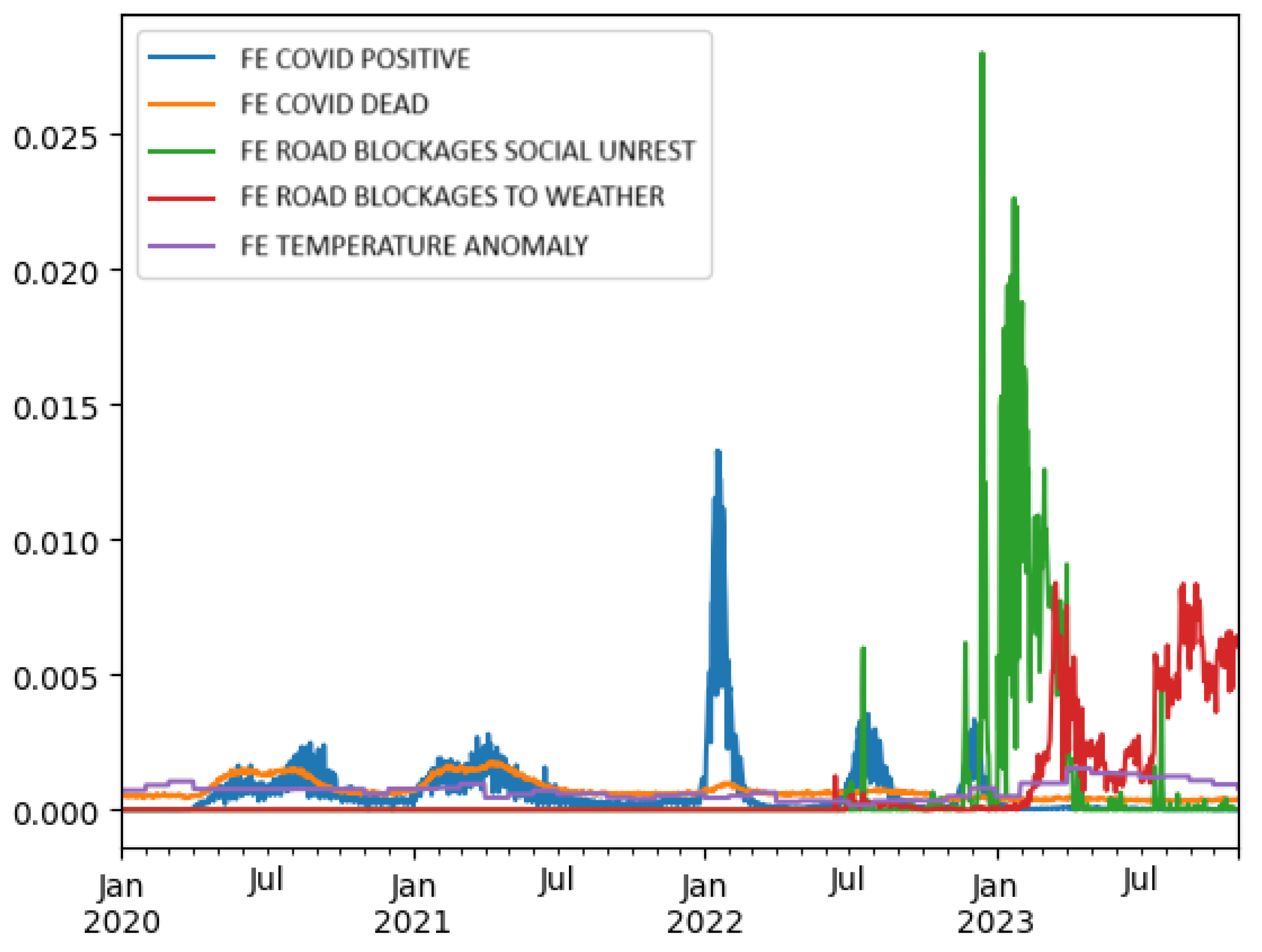
Figure 2.
Adapted CRISP-DM Model for the Analysis of EF.
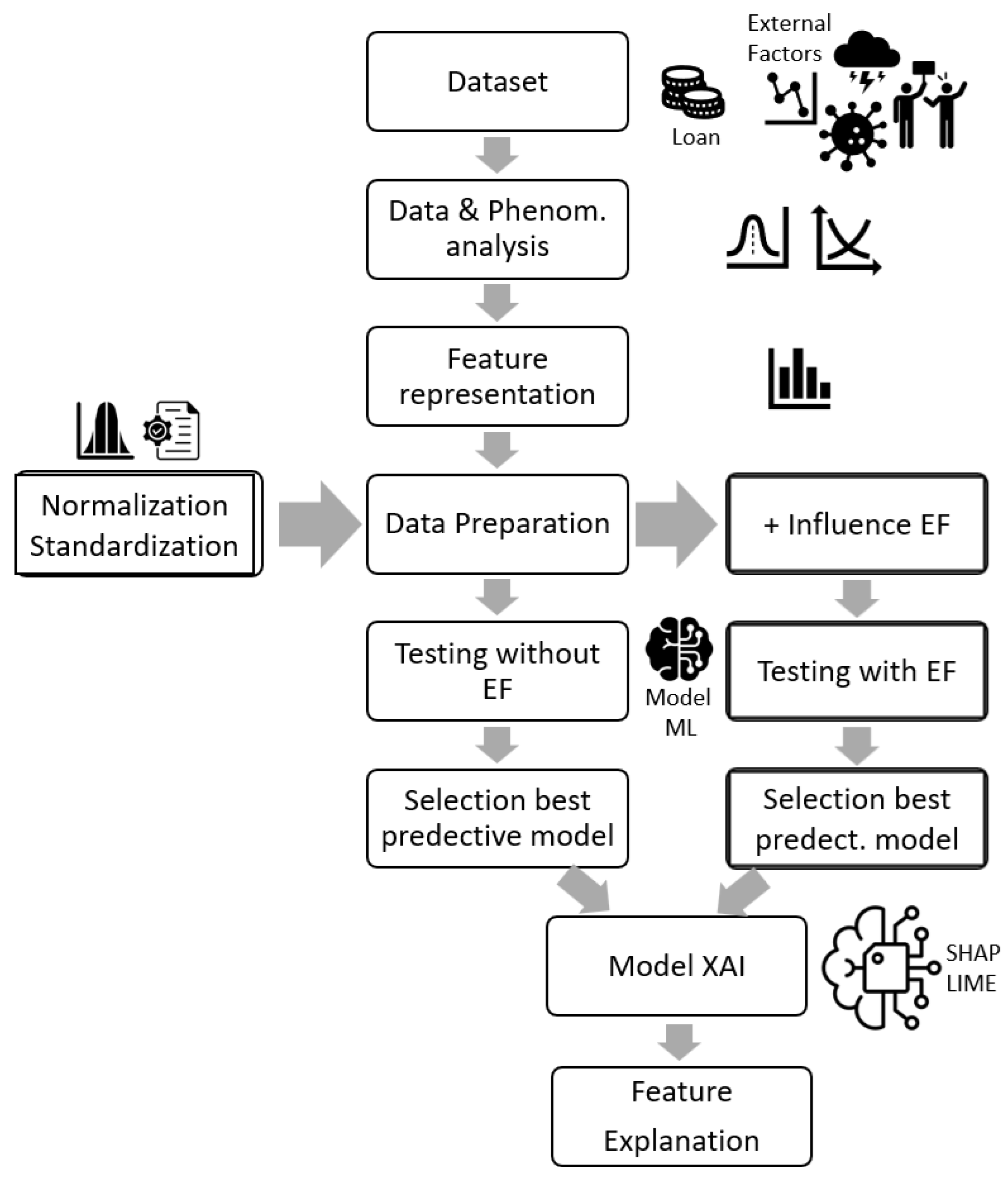
Figure 3.
Impact on Economic Activities by External Factor COVID 19.
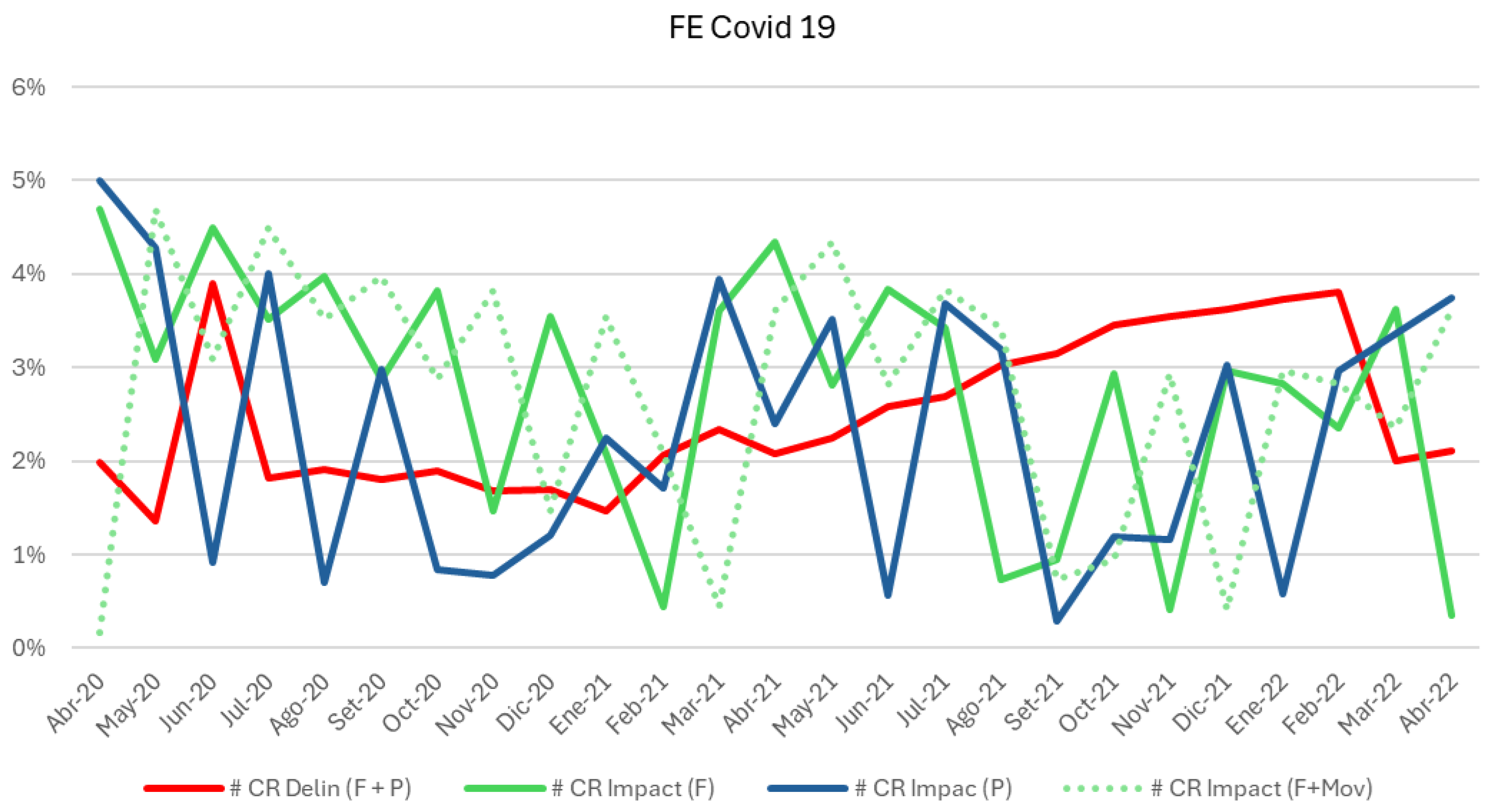
Figure 4.
Impact on Economic Activities by External Factor Social Unrest and Climatic Factors.
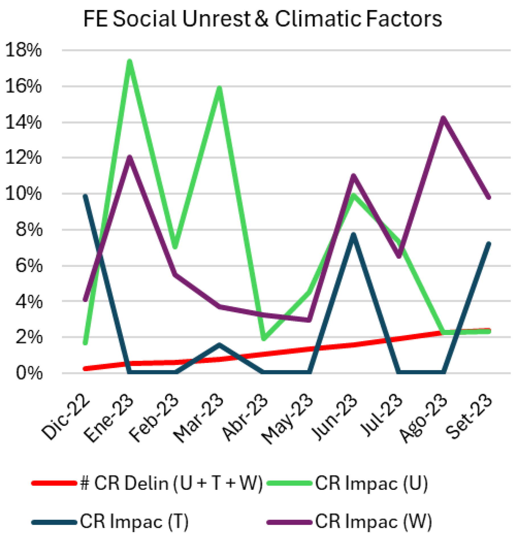
Figure 5.
Relevance of Economic Activity.
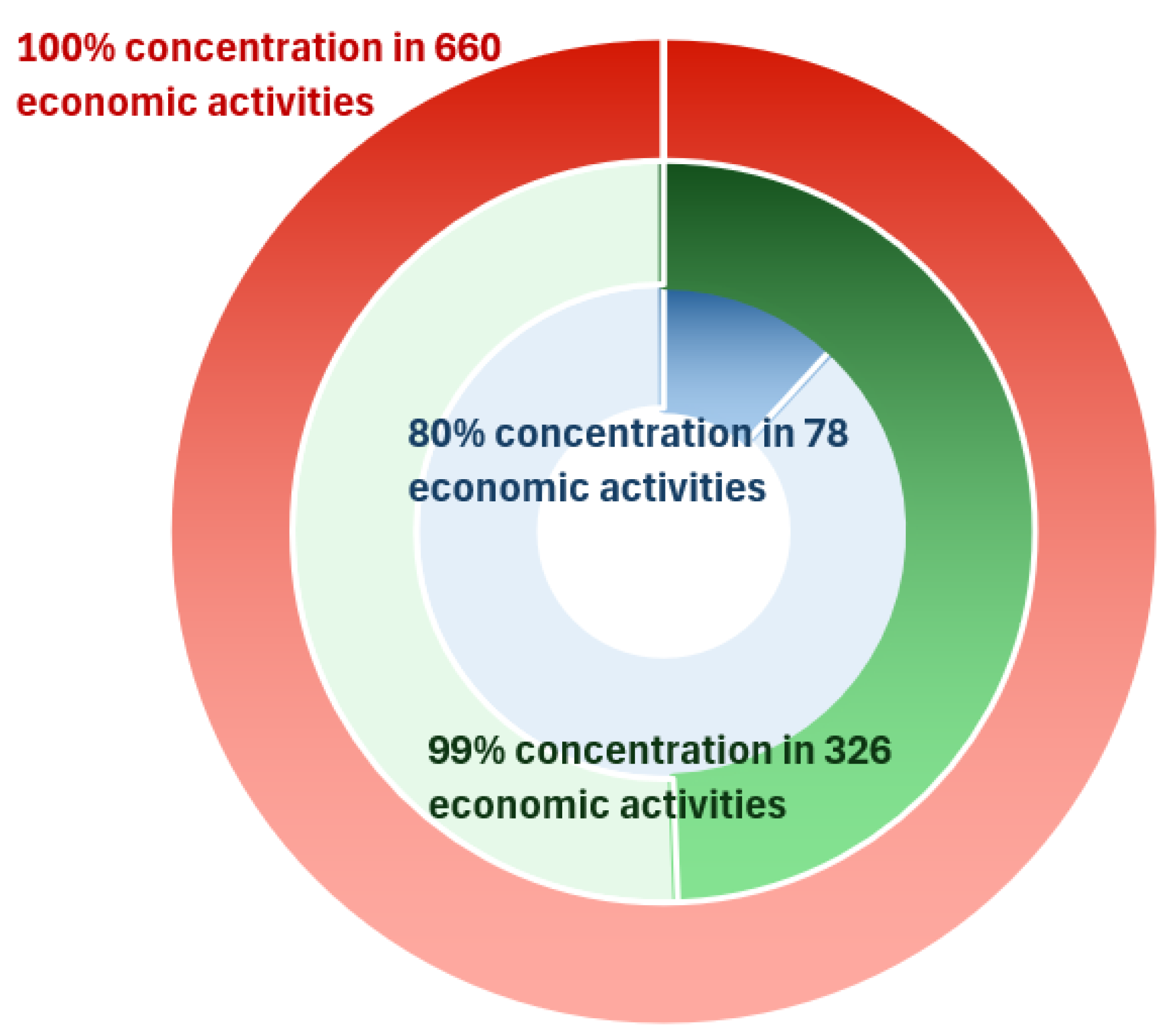
Figure 6.
Top 10 Features between SFE vs F+P scenarios: (a) XNN SHAP Analysis. (b) XNN LIME Analysis. (c) CNN SHAP Analysis. (d) CNN Lime Analysis
Figure 6.
Top 10 Features between SFE vs F+P scenarios: (a) XNN SHAP Analysis. (b) XNN LIME Analysis. (c) CNN SHAP Analysis. (d) CNN Lime Analysis
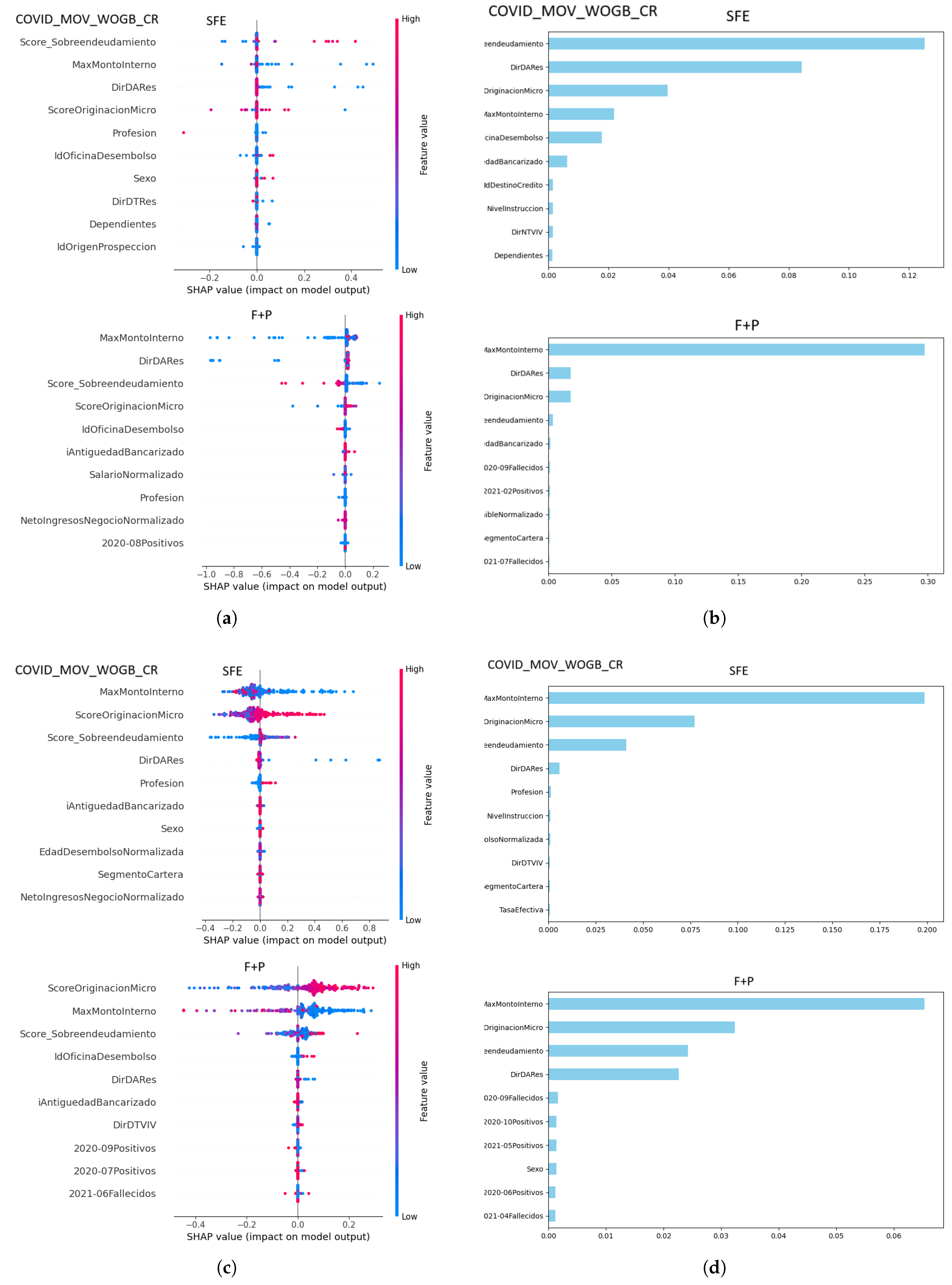
Figure 7.
Top 10 Features between SFE vs T+W scenarios: (a) XGB SHAP Analysis. (b) XGB LIME Analysis.
Figure 7.
Top 10 Features between SFE vs T+W scenarios: (a) XGB SHAP Analysis. (b) XGB LIME Analysis.
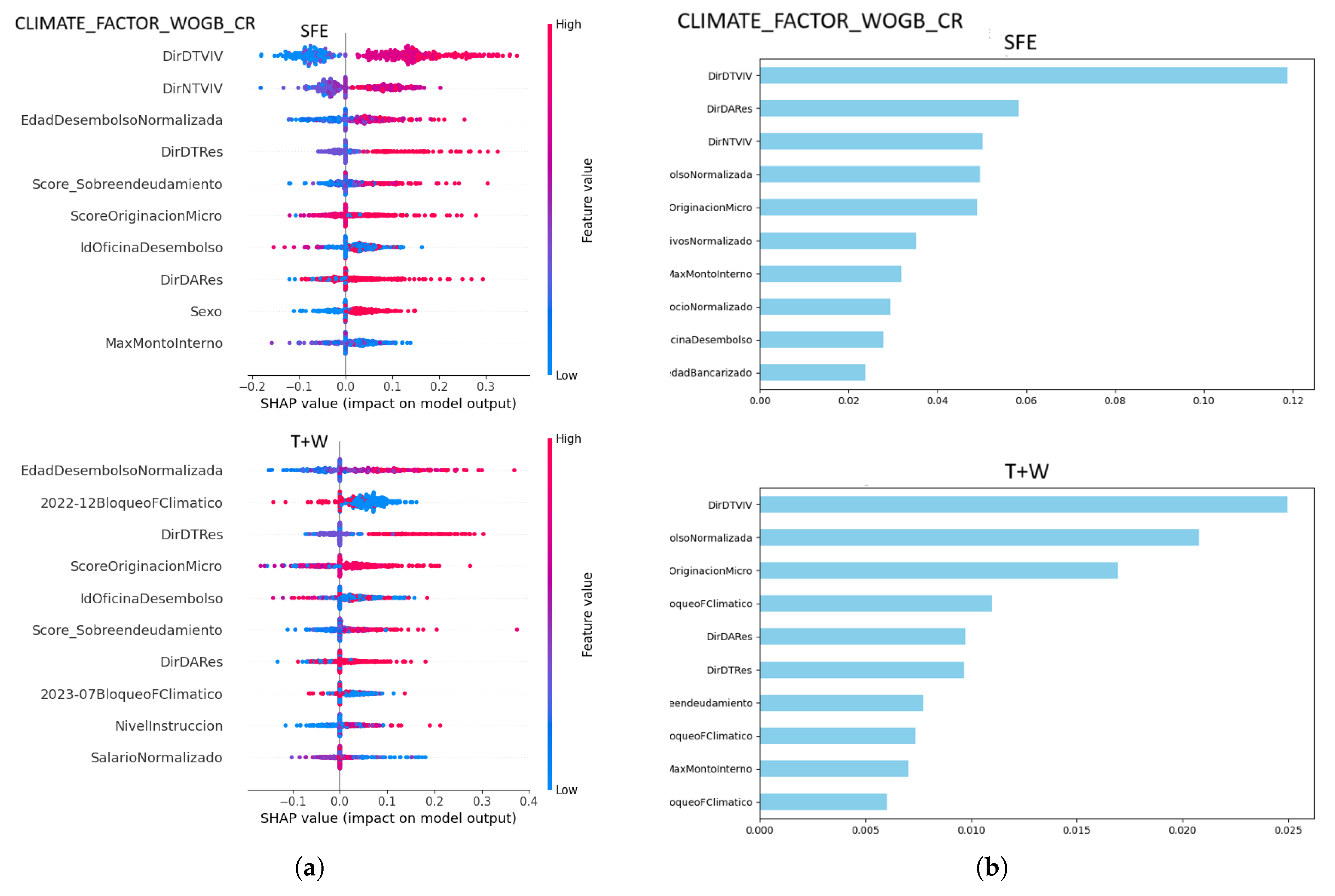
Figure 8.
SHAP XGB & CNN: Top 10 Features between U scenarios.
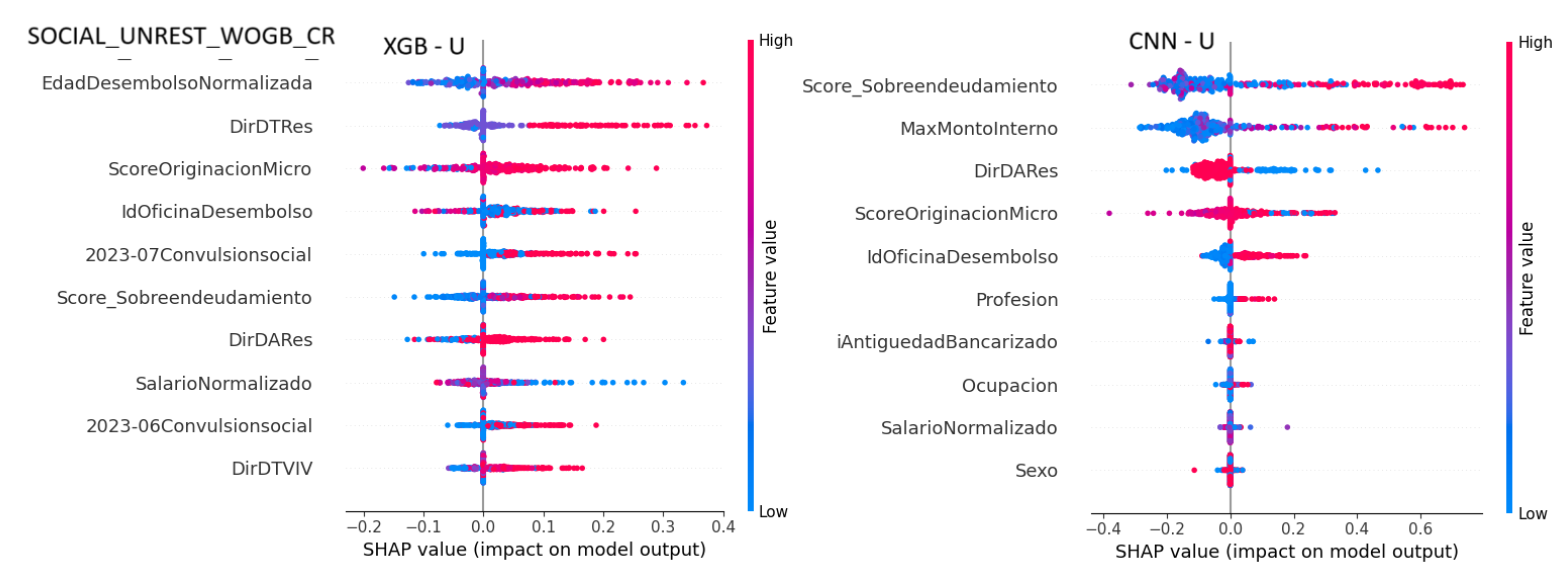
Figure 9.
SHAP CNN, XGB, & XNN: Top 10 Features between U+T+W scenarios.
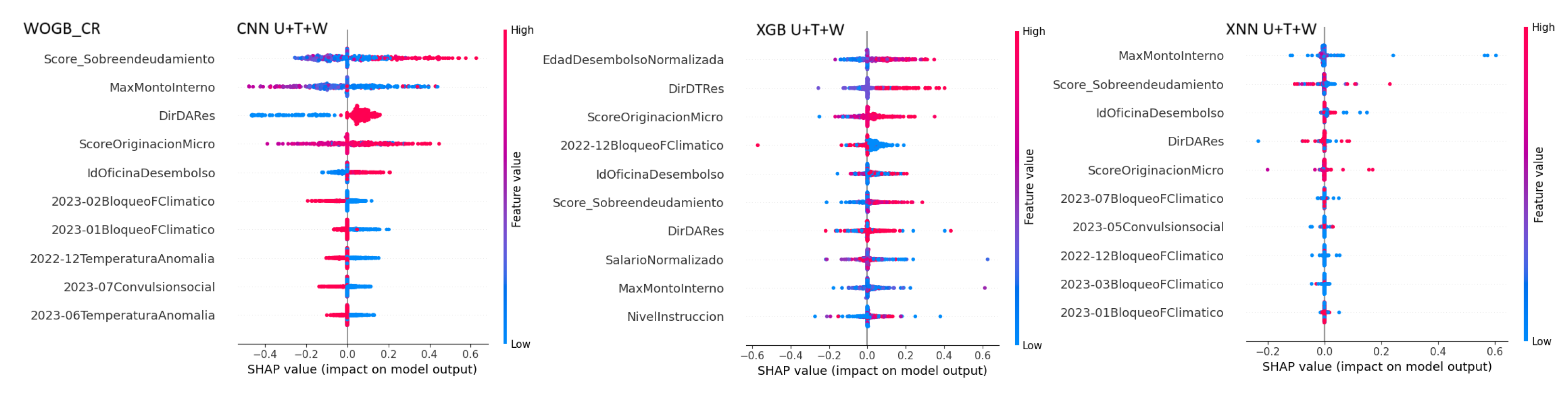
Table 1.
Research Questions.
| ID | QUESTION |
|---|---|
| RQ1 | How did the COVID-19 pandemic, through factors such as positive cases and mortality rates, influence credit defaults in different economic activities? |
| RQ2 | To what extent do climate change indicators, such as temperature anomalies and road blockages due to weather, impact credit delinquency patterns? |
| RQ3 | What is the relationship between credit delinquency and social unrest, considering disruptions to economic activities and societal stability? |
| RQ4 | How do the combined effects of external factors (COVID-19, climate change, and social unrest) contribute to variations in credit delinquency, and what are the most influential factors? |
Note: This table outlines the research questions (RQs) focusing on how external factors such as COVID-19, climate change, and social unrest influence credit default and delinquency patterns. It explored their combined effects and identified the most influential factors.
Table 2.
Datasets.
| It. | DATASET & EF | SOURCE | ROWS |
|---|---|---|---|
| x 1000 | |||
| 1 | COV-19 Positive Cases | https://www.datosabiertos.gob.pe/ | 4,523 |
| 2 | COV-19 Deaths | https://www.datosabiertos.gob.pe/ | 1,064 |
| 3 | Road Blockages | https://www.gob.pe/mtc | 271 |
| 4 | Temperature Anomaly | https://www.senamhi.gob.pe/ | 22 |
| 5 | Delinquency Activity | Model Finance | 1,945 |
| 6 | Credits with EF | Model Finance | 367 |
Note: This table presents the datasets used, including sources and the number of rows (in thousands). The datasets cover COVID-19 cases, deaths, road blockages, temperature anomalies, delinquency activity, and credits with external factors (EF).
Table 3.
Economic Activity Delinquency Stationarity
| Class. | Without EF | With EF | ||
|---|---|---|---|---|
| Eval.Start | 2018.Apr | 2019.Jan | 2020.Apr | 2022.Dec |
| Eval.End | 2020.Feb | 2019.Dec | 2023.Set | 2023.Jun |
| (#) Non-Stat. | 647 | 625 | 465 | 404 |
| (#) Stat. | 49 | 40 | 137 | 29 |
| (#) Indeterm. | 22 | 21 | 15 | 41 |
| (%) Non-Stat. | 90% | 91% | 75% | 85% |
| (%) Stat. | 7% | 6% | 22% | 6% |
| (%) Indeterm. | 3% | 3% | 2% | 9% |
| (#) Total | 718 | 686 | 617 | 474 |
| (%) Total | 100% | 100% | 100% | 100% |
Note: This table compares the economic activity delinquency stationarity with and without external factors (EF) over different evaluation periods. This highlights the proportion of stationary, non-stationary, and indeterminate cases.
Table 4.
Acronyms of Evaluated Scenarios
| Item | Scenario | Acronym |
|---|---|---|
| 1 | Without EF | SFE |
| 2 | EF COVID Dead | F |
| 3 | EF COVID Positive | P |
| 4 | EF COVID Dead & Positive | F+P |
| 5 | EF Social Unrest | U |
| 6 | EF Temperature Anomaly | T |
| 7 | EF Road blockage weather (RBW) | W |
| 8 | EF S.Unrest & Temp.Anomaly | U+T |
| 9 | EF Temp.Anomaly & RBW | T+W |
| 10 | EF S.Unrest & RBW | U+W |
| 11 | EF S.Unrest, Temp.Anomaly & RBW | U+T+W |
| 12 | With govt-backed Credit | WGB_CR |
| 13 | Without govt-backed Credit | WOGB_CR |
Note: This table lists the acronyms for the evaluated scenarios, such as social unrest (U), temperature anomaly (T), and road blockages (RBW). Combined scenarios such as U+T and U+T+W are also defined.
Table 5.
Acronyms of the Results for the Evaluated Scenarios
| Item | Results | Acronym |
|---|---|---|
| 1 | Result F minus SFE | F-S |
| 2 | Result P minus SFE | P-S |
| 3 | Result F+P minus SFE | F+P-S |
| 4 | Result U minus SFE | U-S |
| 5 | Result T minus SFE | T-S |
| 6 | Result W minus SFE | W-S |
| 7 | Result U+T minus SFE | U+T-S |
| 8 | Result T+W minus SFE | T+W-S |
| 9 | Result U+W minus SFE | U+W-S |
| 10 | Result U+T+W minus SFE | U+T+W-S |
Note: This table provides acronyms for the results of evaluated scenarios, comparing the differences between scenarios like "Result F minus SFE" and "Result U+T+W minus SFE." These comparisons are systematically abbreviated for clarity.
Disclaimer/Publisher’s Note: The statements, opinions and data contained in all publications are solely those of the individual author(s) and contributor(s) and not of MDPI and/or the editor(s). MDPI and/or the editor(s) disclaim responsibility for any injury to people or property resulting from any ideas, methods, instructions or products referred to in the content. |
© 2025 by the authors. Licensee MDPI, Basel, Switzerland. This article is an open access article distributed under the terms and conditions of the Creative Commons Attribution (CC BY) license (http://creativecommons.org/licenses/by/4.0/).
Copyright: This open access article is published under a Creative Commons CC BY 4.0 license, which permit the free download, distribution, and reuse, provided that the author and preprint are cited in any reuse.


