Submitted:
23 October 2025
Posted:
27 October 2025
You are already at the latest version
Abstract
Credit risk forecasting in consumer finance must fully account for macroeconomic fluctuations ( ) to ensure portfolio stability and meet regulatory requirements. This study constructs default probability prediction models using logistic regression, XGBoost, and LightGBM based on 5 million credit accounts, then conducts stress testing under macroeconomic scenarios including unemployment rate, inflation, and interest rate shocks. Results indicate that within a 24-month rolling window sample, the XGBoost model achieves an AUC of 0.82, surpassing logistic regression by 7.5%. Under severe recession scenarios, the model accurately captures the trend of default rates rising to 6.3% with an error margin below 0.5%. Simultaneously, stress test results provided portfolio-level Value at Risk (VaR) and Expected Shortfall (ES) intervals, enhancing the robustness of capital adequacy assessments. The study demonstrates that integrating machine learning with macroeconomic scenario analysis strengthens systemic risk monitoring, supports consumer protection, and provides quantitative tools for regulatory stress testing.
Keywords:
credit risk forecasting
; stress testing
; consumer finance
; machine learning
; macroeconomic scenarios
; portfolio stability
1. Introduction
With the rapid evolution of financial markets, credit portfolios are increasingly exposed to multifaceted risks, particularly those driven by macroeconomic fluctuations. Understanding how macroeconomic conditions influence portfolio default rates and developing robust models for risk assessment and stress testing have therefore become central issues in modern credit risk management. By integrating conventional statistical approaches with advanced machine learning techniques, this study establishes a systematic framework for credit risk evaluation and verifies its robustness through stress testing under adverse economic scenarios.
2. Data and Methods
2.1. Data Sources and Preprocessing
This study used 24 months of rolling panel data from 5 million consumer finance accounts. A multi-level dataset was constructed by combining macroeconomic indicators—urban surveyed unemployment rate, Consumer Price Index (CPI), and one-year Loan Prime Rate (LPR). At the micro level, the dataset included borrower profiles, contract terms, credit utilization, repayment behavior, and delinquency migration records. All macro variables were seasonally adjusted, transformed into logarithmic differences, and embedded into monthly panels with optimal lags selected according to AIC and BIC criteria, thereby minimizing potential information leakage [1].The preprocessing stage involved handling missing values, trimming outliers by quantiles, aligning time sequences, and discretizing continuous variables through feature binning and Weight of Evidence (WOE) encoding. Variable selection was based on the Information Value (IV) metric to ensure feature relevance. The WOE definition after binning was expressed as follows:
where Pg,i is the proportion of good samples in group i; Pb,i is the proportion of bad samples. The WOE values for all groups were then aggregated to compute the Information Value (IV), which quantified the discriminative strength of each predictor in default forecasting:
In this analysis, the default label was defined as a loan being 90 days or more past due (90DPD) within the subsequent observation window. By separating the feature construction window from the default observation window, the temporal causality between explanatory and response variables was preserved. Core variables, measurement units, and data sources are summarized in Table 1.
2.2. Model Construction
2.2.1. Logistic Regression Model
The logistic regression model serves as the baseline probability of default (PD) estimator. Inputs comprise WOE-encoded account features selected using an Information Value (IV) threshold of 0.02, yielding 18 final predictors. Each feature was binned by quantile thresholds to maintain monotonic relationships with default rates, and macroeconomic variables were introduced with a one-quarter lag to capture cyclical effects. The model employs L2-regularized maximum likelihood estimation with class weighting and monotonic sign constraints for business consistency. Hyperparameters—regularization strength (C) and class weight balance—were tuned via Time-Series Nested Cross-Validation (TSNCV; five outer and three inner folds) combined with Bayesian Optimization (BO) over the search space C ∈ [0.01, 10] and class_weight ∈ [0.5, 2.0], ensuring temporal stability and avoiding look-ahead bias. Platt calibration was applied to the validation set to correct residual bias [2]. The model’s link function is:
where =σ(·) denotes the Sigmoid function; Yt indicates whether a 90-day default occurred within the observation window; and β,γ represent the micro and macro coefficients, respectively. The objective function with class weights and L2 penalty is:
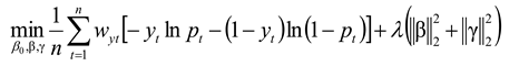
where wyt is the category weight for handling out-of-sample sparsity; λ is the regularization strength; and business monotonicity is specified as a constraint, such as βCUR ≥ 0; βMAXDPD6 ≥0; βINC≥0; γLPR≥0. The calibration mapping is defined as:
where is the uncalibrated PD, and a,b is estimated on the validation set.
2.2.2. XGBoost Model
During model construction, account features encoded via WOE are input alongside lagged macro variables. They first enter a tree model structure constrained by monotonicity to ensure consistency in the directionality of risk factors within business logic. The objective function minimized during training comprises a loss term and a regularization term, expressed as:
where yt denotes the 90-day past due (90DPD) default indicator for account t within the observation window; represents the predicted probability; is the log-loss function; fm is the m th regression tree; and Ω(fm) is the regularization term, which penalizes tree complexity to prevent overfitting. Model training adopted Time-Series Nested Cross-Validation (TSNCV) with five outer and three inner folds to preserve temporal order and prevent data leakage. Hyperparameters were optimized via Bayesian Optimization (BO) within the ranges learning_rate ∈ [0.01, 0.2], max_depth ∈ [3, 10], subsample ∈ [0.6, 1.0], colsample_bytree ∈ [0.5, 1.0], and min_child_weight ∈ [1, 10], ensuring robustness and generalization under time-dependent structures [3]. After prediction, probability outputs were bias-corrected through Platt or isotonic calibration, automatically selected based on validation performance. Macroeconomic shocks were further incorporated through a dynamic adjustment of bias terms, linking changes in unemployment, CPI, and LPR to the model’s internal intercepts. Each macro indicator was standardized over its historical distribution and used to update the baseline bias during prediction, so that shifts in the economic environment directly influenced the probability of default estimation. In this framework, rising unemployment or tightening credit conditions increased the model bias toward higher default probabilities, while improving CPI stability reduced the bias intensity. The resulting bias trajectory captured the gradual drift of credit risk under different macroeconomic regimes. Figure 1 (“Macro Shock Bias Adjustment Diagram”) illustrates the directional effect of macro variables on bias evolution, where unemployment exhibited the strongest and most persistent impact. This mechanism enhanced the model’s interpretability and allowed sensitivity tracing of PD shifts in response to external shocks.
To address temporal correlation in residuals, a block bootstrap with a 10-day block length was applied, smoothing VaR-related fluctuations across time segments. The resulting PD series were then fed into a drift monitoring module, where significant shifts in feature or macro distributions triggered parameter updates and retraining, forming an adaptive closed loop [4]. The overall workflow and feedback mechanism are illustrated in Figure 1, highlighting the interaction between feature embeddings, macroeconomic adjustments, and adaptive retraining.
2.2.3. LightGBM Model
LightGBM is applied alongside XGBoost to improve performance. It uses efficient histogram-based splitting and a leaf-wise growth strategy, balancing training speed and predictive accuracy with large-scale account samples and high-dimensional macro variables. As shown in Figure 2, LightGBM shares XGBoost’s second-order approximation objective but lowers complexity in feature splitting by accumulating gradients and second derivatives through histograms [5]. Its optimization objective is given as:
Where is the first-order gradient, is the second-order derivative, and is the leaf node output; , where T is the number of leaves, wj is the weight of the j th leaf node, and γ,λ is the regularization coefficient. LightGBM employs histogram-based gain calculation during splitting:
where G,H represent the cumulative sums of gradients and second derivatives, respectively, and L,R denote the left and right subintervals. Compared to XGBoost’s point-by-point scanning, LightGBM achieves higher efficiency, especially on rolling panels with 5 million samples [6]. Macroeconomic variables are embedded through lagged expansion, with splits correlated to unemployment, CPI, and LPR prioritized during leaf node growth.Under identical validation folds, XGBoost achieved an Area Under the Curve (AUC) of 0.82 with an average training time of 720 seconds, while LightGBM achieved an AUC of 0.81 with an average training time of 410 seconds. This comparison demonstrated a 43% reduction in training time with only a marginal decrease in classification performance. The results suggest that LightGBM provided a more efficient solution for large-scale, time-dependent credit data without compromising predictive stability.
2.2.4. Model Parameter Optimization
To improve discriminative power and calibration under rolling samples and scenario shocks, parameter tuning combines time-series nested cross-validation (TSNCV) with Bayesian optimization (BO), using multi-objective scalarization as the global criterion [7].The TSNCV structure adopts five outer folds and three inner folds to ensure temporal alignment between training and validation segments, maintaining chronological integrity. Within each inner loop, BO explores the constrained hyperparameter domain defined as learning_rate∈[0.01,0.2], max_depth∈[3,10], subsample∈[0.6,1.0], and min_child_weight ∈[1,10]. The workflow, feedback loop, and constraint gate are shown in Figure 3. Let the hyperparameter vector be and the validation fold set be . For each fold, AUC, expected calibration error (ECE), Brier score, and cross-window KS fluctuation are computed. The multi-objective scalarization integrates these metrics via a weighted aggregation function, dynamically adjusted by validation feedback to balance discrimination and calibration.Penalties apply when monotonic business priors or scenario consistency are violated. The optimization objective is:
Among these, ` ` denotes bin calibration error, ` and `ΔKS ` represent multi-window KS standard deviation; `Vmon` is the penalty for violating the monotonicity constraint `M ` (e.g., `` measures whether PD strain direction and magnitude align with regulatory expectations during macro shocks (UR↑, LPR↑, CPI↑), penalizing deviations by absolute difference); ` ` is the weight selected from the outer validation grid. During optimization, the Tree-structured Parzen Estimator (TPE) algorithm refines the posterior distribution of within prior bounds, and convergence is enforced by an early-stopping rule when the improvement of scalarized objective < 0.001 for five consecutive iterations. Final model calibration is performed via Platt or isotonic mapping, selected adaptively based on ECE minimization.
3. Empirical Analysis
3.1. Macroeconomic Scenario Design
Macro scenarios are built at monthly frequency and aligned with the account panel. The baseline path uses the trend of the past 36 months’ seasonally adjusted series, smoothed by ARIMA/HP filtering while preserving correlations among UR, CPI, and LPR [8]. The adverse scenario applies a 75th percentile shock vector from the 2008–2024 distribution, decaying via an AR(1) process with a six-month half-life and adjusted for multivariate consistency using copulas. The extreme scenario replicates the 95th percentile crisis shocks, adding linkage constraints between policy rates and inflation to ensure statistical validity. All scenarios adopt a 24-month rolling horizon to drive PD mapping and VaR/ES estimates [9].
3.2. Analysis of Stress Test Results
3.2.1. Analysis of Default Probability Changes
In the stress test results, the Probability of Default (PD) shows strong scenario dependency. As shown in Figure 4, under the baseline scenario the portfolio PD remains stable at 3%–4%, consistent with credit quality and macro conditions. Under the adverse scenario, unemployment and CPI shocks drive PD above 5% over the 24-month horizon, underscoring consumer finance sensitivity to contraction [10]. Under the extreme scenario, rising LPR and unemployment push the PD peak to about 6.3%, with persistently high levels, indicating rapid concentration of risk during downturns. These PD dynamics highlight the model’s ability to capture nonlinear shocks and confirm the importance of macro variables in portfolio transmission.
3.2.2. Portfolio Value at Risk (VaR) Measurement.
Based on scenario-based PD mapping, the tail risk of portfolio losses (LLL) is measured over a 24-month horizon. Portfolio loss is defined as
Where EADi is the exposure balance of account i, LGDi is the loss rate at risk (scenario-adjusted for macro factors), and Di is the indicator variable for default status (sampled from calibrated PDs under given scenarios). Portfolio Value at Risk (VaR) is defined at confidence level α as
To mitigate temporal autocorrelation and conditional heteroskedasticity in loss dynamics, a stationary block bootstrap method was employed. Time-ordered residuals were resampled with overlapping windows, using a fixed block length of 10 trading days. The block size was determined through the Ljung–Box test, where the lag-1 autocorrelation coefficient (ρ₁ = 0.36, p < 0.01) confirmed significant serial dependence within approximately two trading weeks. A 10-day block therefore balanced dependence preservation with variance efficiency, avoiding over-smoothing of tail losses while maintaining temporal realism.
A Gaussian copula structure was selected after empirical comparison with Student-t and Clayton copulas, as it provided the lowest Akaike Information Criterion (AIC) and better captured inter-account co-movements under moderate tail dependence. This configuration maintained macro-driven clustering effects while preventing excessive tail thickening, which was observed under the t-copula specification. Consequently, the bootstrap-copula design stabilized VaR estimation and effectively reduced bias caused by serially correlated portfolio losses.
Under the baseline scenario, the loss distribution remained narrow and consistent with historical experience. In adverse conditions, concurrent increases in unemployment (UR) and the loan prime rate (LPR) shifted the distribution rightward and thickened the tail, substantially increasing variance. Under the extreme scenario, both macro shocks produced cumulative amplification, concentrating tail mass beyond the 99th percentile and significantly elevating capital consumption requirements. The resulting stress profile highlighted the nonlinear sensitivity of portfolio risk to macroeconomic co-movements, reinforcing the need for adaptive recalibration under sustained volatility.
3.2.3. Expected Shortfall (ES) Assessment
Stress test results show that portfolio tail risk is more accurately captured by Expected Shortfall (ES). Unlike VaR, which represents loss at a fixed percentile, ES reflects the average loss beyond that threshold, providing a clearer measure of capital adequacy under extreme conditions. Under the baseline scenario, ES and VaR values are nearly identical, indicating a narrow tail and low extreme-risk exposure. In adverse scenarios, rising unemployment and interest rates thicken the tail, causing ES to exceed VaR and revealing larger losses in the extreme region. Under the extreme scenario, portfolio PD peaks at 6.3%, and ES substantially surpasses VaR, signifying a rightward tail shift and losses amplified by concentration effects. These results underscore ES’s effectiveness in capturing tail-risk sensitivity to macroeconomic shocks and its importance as a complement to VaR in capital planning and countercyclical buffer design.
3.2.4. Sensitivity Analysis
Sensitivity assessment follows the chain “macro factors → account PD → portfolio tail losses,” using elasticity and interaction decomposition under nested time-series validation to measure the marginal and joint effects of UR, LPR, and CPI. Figure 5 shows that as shocks intensify, the PD–VaR/ES response shifts from near-linear to convex. The interaction term UR×LPR has strong impact, indicating that rising unemployment and interest rates jointly thicken the tail, reinforced by Copula correlations. Robustness checks across 24-month rolling windows confirm stable elasticity rankings, with drift mainly as curvature shifts at high quantiles. This consistency ensures interpretability across macro phases. Comparing PD paths with VaR bands shows that when UR and LPR rise together, PD peaks and tail quantiles shift rightward, while the ES–VaR gap widens monotonically, reflecting nonlinear amplification of capital needs.
4. Conclusions
This study predicts and stress tests credit risk in consumer finance portfolios under macroeconomic scenarios. Using Logistic Regression, XGBoost, and LightGBM, it evaluates default probability, VaR, and ES dynamics across economic conditions. Results highlight the unemployment–interest rate linkage as a key driver of tail expansion and confirm the advantage of machine learning in capturing nonlinear shocks and systemic risk. Scenario-based calibration and sensitivity analysis further strengthen model robustness and interpretability, offering quantitative foundations for capital adequacy and countercyclical buffer design. Future research should incorporate market liquidity and policy responses into a higher-dimensional macro-financial framework to build a more comprehensive stress testing system.
References
- Abdolshah F, Moshiri S, Worthington A. Macroeconomic shocks and credit risk stress testing the Iranian banking sector. Journal of Economic Studies 2021, 48, 275–295. [Google Scholar]
- Hu, L. Hybrid Edge-AI Framework for Intelligent Mobile Applications: Leveraging Large Language Models for On-device Contextual Assistance and Code-Aware Automation. Journal of Industrial Engineering and Applied Science 2025, 3, 10–22. [Google Scholar] [CrossRef]
- de Oliveira Campino J, Galizia F, Serrano D, et al. Predicting sovereign credit ratings for portfolio stress testing. Journal of Risk Management in Financial Institutions 2021, 14, 229–241. [Google Scholar] [CrossRef]
- Rakotonirainy M, Razafindravonona J, Rasolomanana C. Macro stress testing credit risk: Case of Madagascar banking sector. Journal of Central Banking Theory and Practice 2020, 9, 199–218. [Google Scholar] [CrossRef]
- Gallas S, Bouzgarrou H, Zayati M. Analyzing Macroeconomic Variables and Stress Testing Effects on Credit Risk: Comparative Analysis of European Banking Systems. Journal of Central Banking Theory and Practice 2025, 2, 121–149. [Google Scholar] [CrossRef]
- Kanapickienė R, Keliuotytė-Staniulėnienė G, Vasiliauskaitė D, et al. Macroeconomic factors of consumer loan credit risk in central and eastern European countries. Economies 2023, 11, 102. [Google Scholar] [CrossRef]
- Kanapickienė R, Keliuotytė-Staniulėnienė G, Teresienė D, et al. Macroeconomic determinants of credit risk: Evidence on the impact on consumer credit in central and Eastern European countries. Sustainability 2022, 14, 13219. [Google Scholar] [CrossRef]
- Vangala S R, Polam R M, Kamarthapu B, et al. A Review of Machine Learning Techniques for Financial Stress Testing: Emerging Trends, Tools, and Challenges. International Journal of Artificial Intelligence, Data Science, and Machine Learning 2023, 4, 40–50. [Google Scholar]
- Mongid A, Suhartono S, Sistiyarini E, et al. Historical stress test of credit risk using montecarlo simulation: Indonesia Islamic banking. International Journal of Business and Society 2023, 24, 608–619. [Google Scholar] [CrossRef]
- Horváth, G. Corporate Credit Risk Modelling in the Supervisory Stress Test of the Magyar Nemzefi Bank. Financial and Economic Review 2021, 20, 43–73. [Google Scholar] [CrossRef]
Figure 1.
XGBoost Scenario Embedding—Feature Interaction Transmission Diagram.
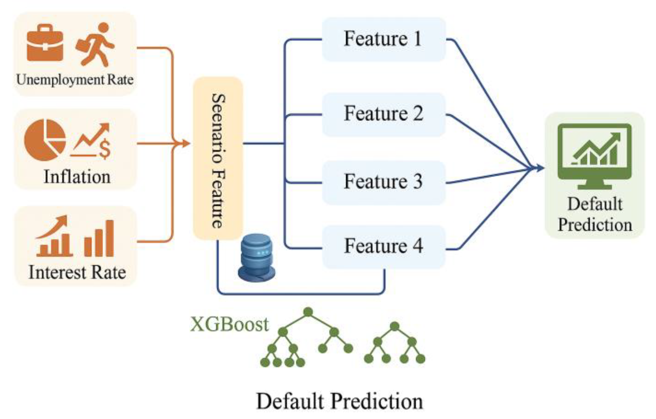
Figure 2.
LightGBM Histogram Splitting and Scenario Injection Path Diagram.
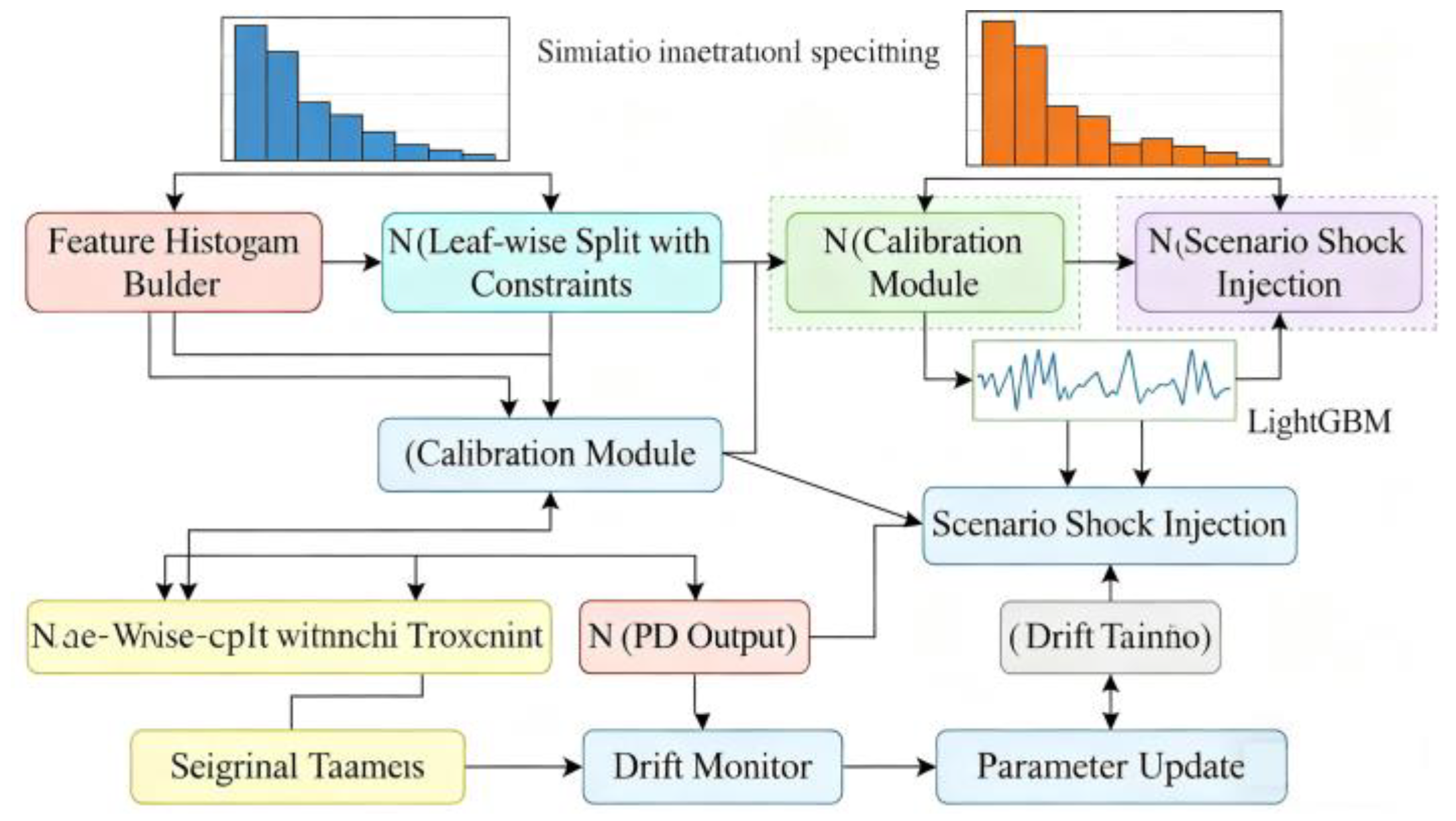
Figure 3.
Parameter Optimization—Scenario Consistency and Calibration Closed-Loop Diagram.
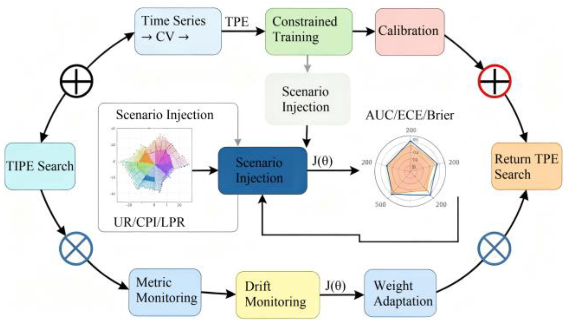
Figure 4.
Dynamic Probability of Default under Stress Testing.
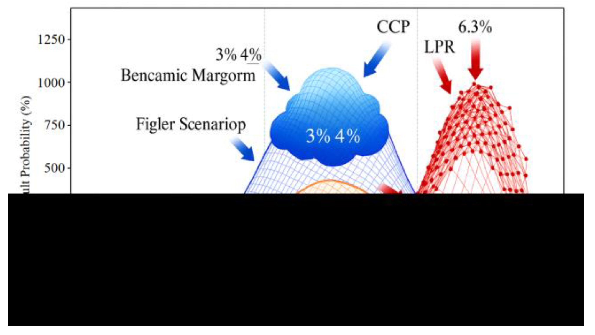
Figure 5.
Scenario Sensitivity Surface and Path Elasticity Diagram.
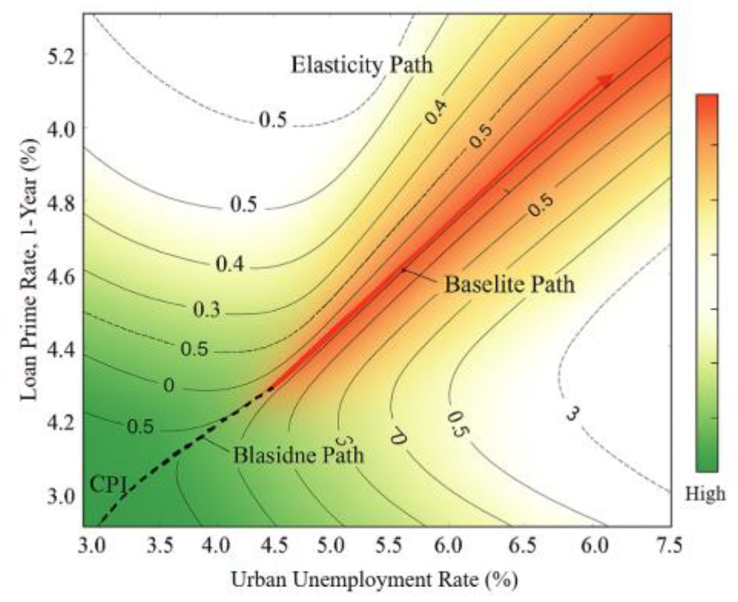

Table 1.
Summary of Sample Data and Macroeconomic Indicators.
| Category | Field/Indicator | Symbol | Value/Definition | Data Source |
| Account Profile | Age/Years | AGE | Natural age at contract signing | Institutional Core System |
| Stable Income (CNY/month) | INC | Pre-tax Monthly Income (Average of Last 3 Months) | Bank Payroll/Tax Filing | |
| Contract Terms | Annualized Interest Rate (%) | APR | Contractually Agreed Annualized Interest Rate | Contract Element Library |
| Behavior Intensity | Credit Utilization Rate/% | CUR | Current month’s used credit/credit limit | Billing System |
| Repayment Behavior | Minimum Payment Ratio/% | MPR | Actual Repayment/Minimum Required Repayment for the Current Month | Billing System |
| Credit Performance | Number of Delinquencies in Last 12 Months/Times | DLQ12 | Rolling 12-Month Count of Delinquencies ≥1 Day | Risk Data Marketplace |
| Maximum Delinquency Days in Last 6 Months/Days | MAXDPD6 | Rolling 6-Month Maximum DPD | Risk Data Marketplace | |
| Target Label | Default Indicator (0/1) | Y | Future Observation Window Reaches 90 DPD | Post-loan System |
| Macroeconomic Factors | Urban Unemployment Rate/% | UR | Monthly seasonally adjusted level | National Statistical Authority |
| CPI YoY (%) | CPIyoy | Monthly YoY Growth Rate | Statistical Bulletin | |
| LPR (1Y)/% | LPR 1Y | Monthly quote, incorporated into the model with lagged stages | Released by the Central Bank |
Disclaimer/Publisher’s Note: The statements, opinions and data contained in all publications are solely those of the individual author(s) and contributor(s) and not of MDPI and/or the editor(s). MDPI and/or the editor(s) disclaim responsibility for any injury to people or property resulting from any ideas, methods, instructions or products referred to in the content. |
© 2025 by the authors. Licensee MDPI, Basel, Switzerland. This article is an open access article distributed under the terms and conditions of the Creative Commons Attribution (CC BY) license (http://creativecommons.org/licenses/by/4.0/).
Copyright: This open access article is published under a Creative Commons CC BY 4.0 license, which permit the free download, distribution, and reuse, provided that the author and preprint are cited in any reuse.


