
Submitted:
19 February 2025
Posted:
20 February 2025
You are already at the latest version
Abstract
Currently, most studies on slope stability either neglect or consider only one of the two critical factors—rainfall conditions and crack state—that influence the stability of newly failed slopes. To address this limitation, the eleven parameters, such as the slope height, internal friction angle, cohesion, rainfall conditions, and crack state were selected as evaluation indexes. GeoStudio software was also used to simulate the slope safety factor under various parameters, and 363 sets of data were obtained. The XGBoost-PSO-SVR (eXtreme Gradient Boosting-Particle Swarm Optimization-Support Vector Regression) model was employed to train the simulation results and construct a predictive model. Compared with the single-machine methods of XGBoost and PSO-SVR, the MSE of XGBoost-PSO-SVR is reduced by 71.9% and 57.8%, respectively. Furthermore, when compared to four single-machine models—Decision Tree (DT), Naive Bayes (NB), Random Forest (RF), and K-Nearest Neighbors (KNN)—the XGBoost-PSO-SVR model demonstrated superior training performance. The predicted safety factor for a newly failed slope in Yongchun County, Fujian Province, during November 4-7, 2016, was 0.9658, which closely aligns with the actual conditions. A new way for the stability prediction of newly failed slope could be provided by this study under various factors, such as rainfall conditions and crack state.
Keywords:
eXtreme Gradient Boosting
; Particle Swarm Optimization Support Vector Regression
; newly failed slope
; red clay
; safety factor
1. Introduction
Among various geological disasters, landslides are characterized by their wide distribution, high frequency of occurrence, and significant damage. Extensive research has been conducted on slope stability analysis, yielding substantial results. However, most studies focus on slopes before sliding occurs. Even though a few scholars have explored the stability of already failed slopes, their research primarily focus on ancient landslides. Such as Yang et al., Hu et al., Zhu et al. and Frink et al. studied the stability of ancient landslides by field survey and monitoring, satellite remote sensing, optical remote sensing dynamic monitoring, drone aerial survey and numerical simulation [1-8]. While these studies have contributed to understanding ancient landslide revival, the shear strength of the sliding zone in newly failed slopes has not been restored, and surface cracks remain unblocked. Consequently, findings from ancient landslide studies cannot be directly applied to newly failed slopes. The stability of the newly failed slope at Xintang Gao Kanzi was analyzed by using the transfer coefficient method [9]. However, only the weight of the slope and the weight under a once-in-50-years heavy rain scenario were considered. The parameters considered were also limited to the natural unit weight, internal friction angle, and cohesion of both the slope and the sliding zone. The hydraulic coupling numerical simulation was used to simulate its stability by Wang et al [10]. But only three kinds of rainfall conditions, such as light rain, moderate rain and heavy rainstorm were considered, without considering the influence of crack state. It is suggested that abundant loose material sources and dominant joint structures could provide fundamental conditions for the transition from shallow to deep sliding of the slope [11]. However, only natural conditions and heavy rainfall scenarios were considered, which was insufficient. The reverse analysis method and cloud model method were used to evaluate the stability of a newly failed slope [12]. But the influence degree of crack length, width, depth and position on the stability of the slope was not considered.
Although the aforementioned analytical methods have their merits, scholars have rarely considered both rainfall conditions and crack states simultaneously, despite their interaction and mutual constraints [13-18]. At present, machine learning has been widely used to predict in various research fields. Models such as Decision Tree (DT) [19], K-Nearest Neighbors (KNN) [20], Naive Bayes (NB) [21], Random Forest (RF) [22], eXtreme Gradient Boosting (XGBoost) [23], and Support Vector Regression (SVR) [24] each have their advantages and disadvantages. For example, the XGBoost model has the advantages of non-linear data processing, low computational load, faster operation speed, and better prevention of overfitting [25-26]. However, it has the disadvantages of easy overfitting and sensitivity to outliers. The SVR model can effectively solve practical issues such as small sample sizes, nonlinearity, high dimensionality, and local minima, demonstrating excellent generalization performance [27-28]. However, it suffers from slow training and difficult parameter selection. It was believed that combining multiple single machine learning models can yield a predictive model with superior performance [29-31].
The study selected 11 parameters commonly used for red clay slope evaluation, including slope height, slope angle, cohesion, internal friction angle, rainfall conditions, and crack status. The safety factor of the slope under different parameter values was simulated and analyzed using GeoStudio software. Subsequently, an adaptive weighted XGBoost-PSO-SVR hybrid model was trained with the simulation results to establish a prediction model. The model's effectiveness of this model was verified by comparing its prediction results with those of single machine learning models like XGBoost, PSO-SVR, and DT. Finally, the model's accuracy was further validated through a case study of a recently failed slope in Yongchun County, Fujian Province. This study provided a new approach for the stability prediction of recently failed slopes under comprehensive consideration of various factors, such as rainfall conditions and crack status.
2. Materials and Methods
2.1Acquisition of Research Data
To obtain the safety factor of recently failed red clay slopes under rainfall conditions, a finite element model was established using GeoStudio software for numerical simulation. The slope soil assumed to be a single layer of red clay. Since recently failed slopes have numerous and scattered cracks, it would be a huge task to represent all the cracks in the model. Therefore, the cracks were simplified into three main types: the main crack in the slip zone, the crack at the top of the slope, and the crack on the slope surface, respectively. The length and width of the main crack in the slip zone could be equivalently processed using Equation 1 and 2. The length of the cracks at the top and surface of slope was calculated as half of the main crack length, and their width could be equivalently processed using Equation 3.
(1)
(2)
(3)
Where Lm is the equivalent length of the main crack; li is the length of each crack in the slip zone; xi is the horizontal distance of each crack from the center of the slip zone; Dm is the equivalent width of the main crack; di is the width of each crack. Dn is the equivalent width of the cracks at the top of the slope or on the surface of slope; Si is the area of each crack at the top of the slope; S is the total area of the top of the slope; L is the length of the top of the slope.
Since the study focused on recently failed slopes, a slip zone was assumed to exist. Therefore, the most dangerous slip surface of the single-layer homogeneous soil in the model was set as the slip zone. However, whether the final slip surface passed through this slip zone was determined by the numerical simulation of GeoStudio software, without forcing the slip surface to pass through the slip zone in this simulation. Taking a model with slope height of 10 meters and slope angle of 45° as an example, the final model was shown in Figure 1. In the figure, N1 represented the red clay layer base; N2 was the recently failed red clay layer; H1was the slip zone; L1 was the main crack in the slip zone; L2 was the crack at the top of the slope; L3 was the crack on the surface of slope; W1 was the groundwater level. The constitutive model of this model was selected as the Mohr-Coulomb model. Since the rainfall intensity in this simulation was relatively high, for the good infiltration channel cracks and slip zone soil, the rainfall intensity was set as a flow boundary. But for the red clay layer without cracks, the rainfall boundary condition was set as a zero-pressure water head boundary. The seepage in this model was transient seepage, and the influence of groundwater was not considered. Therefore, the groundwater level was set as close to the bottom of the slope as possible, as shown in the position of W1 in Figure 1.
The parameters selected for simulation included slope height (H), slope angle (β), cohesion (c), internal friction angle (φ), unit weight (γ), rainfall intensity (Ir), rainfall duration (Tr), main crack width (Dm), main crack depth (Lm), crack area ratio at the top of the slope (St), and crack area ratio on the surface of slope (Sf). According to the Engineering Geology Manual, the minimum unit weight of red clay is 16.5 kN/m³, and the maximum is 18.5 kN/m³. The benchmark values for the three groups were selected as 17.0 kN/m³, 17.5 kN/m³, and 18.0 kN/m³ using the equal division method. The grouping benchmark values for internal friction angle and unit weight were selected in the same way. The meteorological department defines rainfall less than 10 mm in 24 hours as light rain, between 10 mm and 25 mm as moderate rain, and between 25 mm and 50 mm as heavy rain. Therefore, 10 mm, 25 mm, and 50 mm were selected as the benchmark values for each group. For parameters such as slope height, slope angle, and rainfall duration, the benchmark values were selected based on the common classification standards used by scholars. The final benchmark values for each group of parameters were shown in Table 1. The safety factor of the slope was then calculated for different combinations of conditions in each group, with each parameter varying by ±5%, ±10%, ±15%, ±20%, and ±25% of its group benchmark value. For example, the combinations of conditions for Group II were shown in Table 2.
The density, cohesion, and internal friction angle of the cracks in this numerical simulation were all set to zero. The density of the slip zone soil was taken to be consistent with the density of the red clay being simulated. The cohesion and internal friction angle of the slip zone soil were referenced from the research results of Tang [32] and Ren [33], and were set at 19.5 kPa and 10.73°, respectively. The slope model was set as unsaturated, and the sample material was selected from the built-in clay material of GeoStudio software. The saturated and residual water content of the soil were both set at 45% and 10%, respectively. The permeability coefficients of red clay, slip zone soil, and cracks were taken as 5×10⁻¹⁰ m/s, 5×10⁻⁶ m/s, and 1 m/s, respectively. The relationship curves of matric suction with volumetric water content and water X-conductivity of the slip zone soil were shown in Figure 2 and Figure 3, respectively.
According to the above simulation scheme and parameter values, numerical simulations were conducted using GeoStudio software. Since the safety factor of the slope dynamically changes during rainfall, the safety factor obtained in this simulation was the one at the last moment of the rainfall duration. A total of 363 sets of simulation results were obtained, and a part of the results from Group II were shown in Table 3.
2.2. XGBoost
XGBoost is an algorithm based on decision trees, with decision trees being its fundamental components. During the decision tree process, subsequent trees are trained based on the residuals of the previous tree. Through continuous iterative optimization, the residuals are minimized, ultimately enhancing the overall model's prediction accuracy. The objective function of the XGBoost model consists of a loss function and a regularization term, calculated according to Equation 4 [34].
(4)
where O is the objective function; yi is the measured value of the i target; is the predicted value of the i target; l(yi, ) is the difference between yi and ; n is the number of samples; Ω(fk) is the complexity of the tree model for the k sample feature parameter fk; k is the number of sample feature parameters.
The objective function was approximated by performing a second-order Taylor expansion on it, thus transforming Equation 4 into Equation 5.
(5)
where gi and hi are the first and second derivatives of , respectively.
Since the goal of the model was to minimize the objective function, the constant term was temporarily disregarded. After removing the constant term and C from Equation 5 and summing the objective function in the form of leaf nodes, Equation 6 was obtained [35].
(6)
where I is the set of samples on each leaf; wj is the output score of each tree leaf node; T is the number of leaf nodes of the split tree; λ and γ are weight factors, controlling the weights of the corresponding parts.
2.3. SVR
SVR is a small-sample creative machine learning method based on statistical learning theory, aiming to minimize the model's structural risk. When dealing with nonlinear problems, this learning method maps the original data x to a high-dimensional feature space to obtain φ(x), thereby transforming it into a linear problem for solution. It has strong generalization performance and is effective for regression problems. Suppose there exists a training set {(xi,yi)|i=1,2,3, ∙∙∙,n}, where xi is the input vector, yi is the output target, and n is the number of samples. The input vector and output target can be described by Equation 7 [36].
(7)
where f(x)is the predicted value; wT is the weight vector; φ(x) is the mapping of the input variable x in the high-dimensional feature space; b is the threshold.
After a series of transformations and the introduction of the Lagrange function and kernel function, the objective function and kernel function of SVR were shown in Equations 8 and 9 [37].
(8)
(9)
where αi and αi* are Lagrange multipliers; K(xi,xj) is the kernel function; ∥xi−xj∥2 is the squared Euclidean distance between two feature vectors; σ is the width of the kernel function; g is the parameter of the kernel function.
C is the penalty coefficient of SVR, mainly used to control the error range of the model to avoid underfitting or overfitting; g is the kernel parameter, mainly used to control the distribution of data in the new feature space, determining the number of support vectors, and thereby affecting the speed of training and prediction. Therefore, determining the optimal parameters is a crucial part of the SVR algorithm [38].
2.4. PSO Algorithm
The PSO algorithm, proposed by Kennedy [39] and Eberhart [40], is a search algorithm inspired by the foraging behavior of birds. It is characterized by its high efficiency and fast search speed. The algorithm mainly iteratively calculates the initial position and velocity of a group of random particles to find the optimal solution [41]. Before the algorithm runs, a group of particles with vector dimension n is initialized. The position of a particle can be denoted as a point in an n-dimensional search space, with its coordinates represented as xi=(xi,1,xi,2,∙∙∙,xi,D), which is also considered a solution in the n-dimensional optimization space. Its flight velocity is denoted as vi=(vi,1,vi,2,∙∙∙,vi,D); the historical optimal coordinates of the i particle are Pi=(Pi,1,Pi,2,∙∙∙,Pi,D); and the optimal coordinates experienced by each particle are Pg=(Pg,1,Pg,2,∙∙∙,Pg,D). During the flight process, the particle swarm can iteratively calculate, as shown in Equations 10 and 11 [42].
(10)
(11)
where m is the size of the particle swarm; D is the dimension of the particle swarm; vkid is the velocity; xkid is the position; k is the iteration number; c1 and c2 are acceleration factors, controlling the state of particles maintaining pbest and gbest; r1 and r2 are random numbers between [0,1]. ω is the inertia weight, used to control the influence of the original speed on the new speed. When ω is large, the algorithm has strong global search capability, and vice versa, it has strong local search capability, which can be expressed by Equation 12.
(12)
where k is the current iteration step; kmax is the maximum iteration step; ωmax and ωmin are the maximum and minimum values of ω, respectively.
2.5. Adaptive Weighting Combination Model
The adaptive weighting combination model is an improvement based on the residual weighting method. Its main approach is to assign weights to the current sample model based on the average weight of the previous m samples [19]. The optimal m needs to be determined through trial calculations, which can be done using Equations 13 to 15.
(13)
(14)
(15)
where is the predicted value of the i sample of the combination model; is the predicted value of the i sample of the j model; ωj(i) is the residual weighting combination model weight of the j model for the i sample; is the sum of squared prediction errors of the j model for the k sample; is the adaptive weighting combination model weight.
3. Results and Discussion
3.1. Comparison of Prediction Results of PSO-SVR, XGBoost, and XGBoost-PSO-SVR
The 363 simulation results were input into the PSO-SVR and XGBoost models for training. Both models had 290 training samples and 73 testing samples. The kernel functions of SVR mainly include linear kernel, polynomial kernel, Gaussian kernel, and Sigmoid kernel. The Gaussian kernel was chosen for SVR due to its ability to handle complex non-linear problems. The PSO algorithm was used to optimize the penalty coefficient C and parameter g with 5-fold cross-validation. According to the experience of scholars, the particle swarm size N in the PSO algorithm was set to 50, the inertia weight ω to 1.2, and the learning factors c1 and c2 to 2, with the maximum iteration number Gkset to 60. The parameter settings for the XGBoost model were shown in Table 4. Based on the above parameter settings, the prediction results for PSO-SVR and XGBoost were obtained. The adaptive weighting combination model was then used to combine these two results, yielding the prediction results for XGBoost-PSO-SVR. The results were shown in Figure 4.
From Figure 4, it could be intuitively seen that when trained using the XGBoost method, two samples had significant deviations between predicted and actual values, while the predicted values of other samples were quite close to the actual values. The mean squared error (MSE) of the test set for this method was 0.0056979, with a corresponding R2 of 0.98378, indicating that the model trained using the XGBoost method could explain 98.4% of the variance in the dependent variable. This demonstrated that the training effect of this model was good. From Figure 5, it could be seen that when trained using the PSO-SVR method, three samples had significant deviations between predicted and actual values. The corresponding MSE and R2 were 0.0037367 and 0.98515, respectively, indicating that this method reduced the MSE by 34.4% compared to the XGBoost method, resulting in better training performance. From Figure 6, it can be seen that when using the XGBoost-PSO-SVR combined algorithm, only one sample had a significant deviation between predicted and actual values, and the fit of the predicted values to the actual values was higher than the above two methods. The corresponding MSE and R2 were 0.0016001 and 0.9919, respectively. It representing a 71.9% reduction in MSE and a 0.83% increase in the accuracy of the dependent variable explanation compared to the XGBoost method; and a 57.8% reduction in MSE and a 0.69% increase in the accuracy of the dependent variable explanation compared to the PSO-SVR method. Therefore, the XGBoost-PSO-SVR combined algorithm could further reduce the model's MSE and improve accuracy, resulting in the best fit. In MATLAB software, the tic and toc functions were used to calculate the start and end times of the algorithm, respectively, to determine the algorithm's execution time. The calculated execution times for PSO-SVR, XGBoost, and XGBoost-PSO-SVR were 8.14 s, 6.21 s, and 13.32 s, respectively. It can be seen that XGBoost has the fastest computation time, while XGBoost-PSO-SVR has the slowest. Since the XGBoost-PSO-SVR algorithm includes the running time of the XGBoost algorithm, the optimization time of the PSO algorithm, and the prediction time of SVR, its running time was longer than that of the individual XGBoost or PSO-SVR algorithms. However, since the data volume analyzed in this case was relatively small and the running times were all relatively short, they were within an acceptable range. If the data volume to be analyzed is larger, the appropriate algorithm should be selected by considering factors such as accuracy and running time.
3.2. Comparison of Prediction Results of XGBoost-PSO-SVR with Other Machine Learning Models
To further verify the prediction accuracy of the XGBoost-PSO-SVR combination model, four single machine learning models, namely DT, KNN, NB, and RF, were used to predict the safety factor. The comparison of the predicted safety factor values with the actual values obtained from these four machine learning models was shown in Figure 7. The MSE and R2 of the safety factor prediction results of the XGBoost-PSO-SVR combination model and the four single machine learning models were shown in Table 5.
From Figure 7 and Table 5, it could be seen that the XGBoost-PSO-SVR model had the smallest MSE, followed by the DT model, and the KNN model had the largest; the XGBoost-PSO-SVR model had the largest R2, followed by the DT model, and the KNN model had the smallest. Therefore, the training effects of the five models, from highest to lowest, were: XGBoost-PSO-SVR, DT, NB, RF, and KNN. Considering the characteristics of each machine learning model, the main reasons were as follows: The DT model usually assumed independence between attributes during construction, but in reality, the factors affecting the slope safety factor were intercoupled; the performance of the KNN model was easily affected when the number of samples of different categories varies greatly, and the samples in this case include parameters from three different groups; the NB model also assumed independence between attributes; the RF model might be affected by the majority class samples, leading to a decrease in the prediction performance of the model for minority class samples, which might occur when the model randomly assigned training and testing samples. SVR was good at handling high-dimensional data and could effectively solve nonlinear classification problems through kernel trick techniques, and the sample dimension in this case was 11, which was suitable for this model. Meanwhile, XGBoost constructed a strong learner by integrating multiple decision trees, and this integration method allowed XGBoost to significantly improve prediction accuracy. Therefore, the training effect of the XGBoost-PSO-SVR model on this sample was the best.
4. Justification
Taking a recently failed slope in Lengshuicun, Yongchun County in China, as reported in [12], the XGBoost-PSO-SVR model established in this paper was used for comparison. Since the opening width at the rear edge of the slide mass of this slope was approximately 0.3 to 1 m, the main crack width was taken as 1.0 m. Also, since the rear edge of the slope body has already moved down as a whole by about 2 to 2.5 m, the main crack depth was taken as 2.5 m. Since there was rainfall from November 4 to 7, 2016, with a total rainfall of 126.1 mm, the rainfall duration was taken as 4 days, and the rainfall intensity was taken as 31.525 mm/day. According to the field investigation, as shown in Figure 8 and Figure 9, the crack area ratio at the top of the slope was estimated to be 20%, and the crack area ratio on the surface of slope was taken as 10%. The values of the other parameters were shown in Table 6.
The parameters listed in Table 6 were input into the XGBoost-PSO-SVR model for prediction, and the results were shown in Figure 10.
From Figure 10, it could be seen that the model predicted the 74th sample for this slope, with a value of 0.966. According to the Technical Code for Building Slope Engineering of Chia (GB50330-2013), the stability state of this slope was unstable. According to the reference [12], the soil at the front edge of the slope moved forward by about 0.5 m from November 4 to 7, verifying the accuracy of the XGBoost-PSO-SVR model. The safety factors obtained by using XGBoost, PSO-SVR, DT, KNN, NB, and RF for this slope were shown in Table 7.
The numerical analysis of this slope using GeoStudio software yielded a safety factor of 0.988. From Table 7, it could be seen that the deviation between the predicted value obtained by XGBoost-PSO-SVR and the numerical analysis value was 0.022. Although this deviation was larger than that of XGBoost and DT, the prediction values of XGBoost and DT were both greater than 1. According to the Technical Code for Building Slope Engineering of Chia, the stability state of this slope should be judged as under stable, which did not match the actual situation of the slope sliding again. Therefore, in general, compared with other methods, the prediction of XGBoost-PSO-SVR was closer to the actual situation.
5. Conclusions
(1) By comparing the MSE and R2 indicators of the models, the XGBoost-PSO-SVR combined algorithm reduced the mean squared error by 71.9% and 57.8% compared to the single XGBoost and PSO-SVR methods, respectively, and increased the accuracy of the dependent variable explanation by 0.83% and 0.69%, respectively. This model had significant advantages in training accuracy and fitting effect. Moreover, compared with the four single models DT, NB, RF, and KNN, the XGBoost-PSO-SVR combined algorithm also achieved the best training effect.
(2) Using the XGBoost-PSO-SVR combined algorithm to predict the stability of a recently failed slope in Lengshuicun, Yongchun County, from November 4 to 7, 2016, the predicted safety factor was 0.966, indicating that the slope was in an unstable state. This prediction result was consistent with the actual situation.
(3) Due to the limitation of workload, this study simplified the cracks on the slope in the numerical simulation, considering only the main crack in the slip zone, the crack at the top of the slope, and the crack on the surface of slope. At the same time, the influence of groundwater and the spatial variability of slope parameters were not considered, which may cause some differences from the actual situation. Future research will focus on more reasonably considering the impact of the above factors on the stability of recently failed slopes.
Author Contributions
Conceptualization, C.Z.; data curation, D.Z.; investigation, G.L.; resources, F.W. All authors have read and agreed to the published version of the manuscript.
Funding
This research was funded by Natural Science Foundation Project of Fujian Provincial for the research project, grant number 2023J011130.
Data Availability Statement
The raw data supporting the conclusions of this article will be made available by the authors on request.
Conflicts of Interest
The authors declare no conflicts of interest.
Abbreviations
The following abbreviations are used in this manuscript:
| XGBoost | eXtreme Gradient Boosting |
| PSO | Particle Swarm Optimization |
| SVR | Support Vector Regression |
| DT | Decision Tree |
| NB | Naive Bayes |
| RF | Random Forest |
| KNN | K-Nearest Neighbors |
| MSE | Mean Squared Error |
References
- Yang, X.; Zhu, P.; Dou, X.; Yuan, Z.; Zhang, W.; Ding, B. Resurrection deformation characteristics and stability of Jiangdingya ancient landslide in Zhouqu, Gansu Province. Geological Bulletin of China 2024, 43, 947–957. [Google Scholar]
- Hu, G.; Liu, W.; Yan, Y.; Fan, X.; Zhang, Y.; Du, G.; Xiong, H.; Wang, M.; Yu, T. Reactivation characteristics and river blocking outburst simulation analysis of Sela ancient landslide in the upper reaches of Jinsha River. Acta Geologica Sinica, 2024. [CrossRef]
- Zhu, S.; Yin, Y.; Tie, Y.; Sa, L.; Gao, Y.; He, Y.; Zhao, H. Deformation characteristics and reactivation mechanism of giant ancient landslide in Wumeng mountain area: a case study of the Daguan ancient landslide. Chinese Journal of Geotechnical Engineering, 2024. [Google Scholar]
- Frink, N.T.; Pirzadeh, S.Z.; Parikh, P.C.; Pandya, M.J.; Bhat, M.K. Resurrection mechanism of retrogressive ancient landslide under cutting action: an example of an ancient landslide on National Way S206. Science Technology & Engineering 2023, 23, 15002–15009. [Google Scholar]
- Fabrizio, B.; Guido, A.; Domenico, A.; Piero, F.; Matteo, G.; Gilberto, P. Landslide susceptibility analysis with artificial neural networks used in a GIS environment. Advances in Science, Technology and Innovation 2024, 18, 291–294. [Google Scholar]
- Liu, T.; Zhang, M.; Wang, L.; Yang, L.; Yin, B. Formation and evolution mechanism of the ancient landslide and stability evaluation of the accumulation body in Jiangdingya, Zhouqu County, Guansu Province. Bulletin of Geological Science and Technology 2024, 43, 266–278. [Google Scholar]
- Zhao, W.; Cao, J.; Guo, C.; Liu, J.; Yang, Z.; Wei, C.; Wu, R. Developmental characteristics and stability simulation of Yangpo Village large-scale ancient landslides in Minxian County,Gansu Province. Geological Bulletin of China 2024, 43, 1869–1880. [Google Scholar]
- Qiu, Z.; Guo, C.; Wu, R.; Jian, W.; Ni, J.; Zhang, Y.; Min, Y. Development Characteristics and Stability Evaluation of the Shadingmai Large-scale Ancient Landslide in the Upper Reaches of Jinsha River,Tibetan Plateau. Geoscience 2024, 38, 451–463. [Google Scholar]
- Zhou, H.; Xiao, Q.; Peng, Y.; Li, C.; Qiu, Q. Stability analysis and engineering control plan optimization for secondary landslide of Gaokanzi in Enshi Xintang. Journal of Shenyang University: Natural Science 2020, 32, 147–152. [Google Scholar]
- Wang, K.; Chang, J.; Li, X.; Zhu, W.; Lu, X.; Liu, H. Mechanistic analysis of loess landslide reactivation in northern Shaanxi based on coupled numerical modeling of hydrological processes and stress strain evolution: A case study of the Erzhuangke landslide in Yan’an. The Chinese Journal of Geological Hazard and Control 2023, 34, 47–56. [Google Scholar]
- Wang, J.; Cheng, Q.; Li, X.; Liu, N.; Zhang, P. Deformation and instability analysis of the transformed secondary landslide—a case of the RK24 landslide in Yuqing-Kaili expressway. Science Technology and Engineering 2020, 20, 89–95. [Google Scholar]
- Chen, Z.; Dai, Z.; Jian, W. Cloud model for stability evaluation of recently failed soil slopes based on weight inversion of influencing factors. The Chinese Journal of Geological Hazard and Control 2023, 34, 125–133. [Google Scholar]
- Zhang, L.; Jiang, X.; Sun, R.; Gu, H.; Fu, Y.; Qiu, Y. Stability analysis of unsaturated soil slopes with cracks under rainfall infiltration conditions. Computers and Geotechnics 2024, 165, 105907. [Google Scholar] [CrossRef]
- Tang, L.; Yan, Y.; Zhang, F.; Li, X.; Liang, Y.; Yan, Y.; Zhang, H.; Zhang, X. A case study for analysis of stability and treatment measures of a landslide under rainfall with the changes in pore water pressure. Water 2024, 16, 3113. [Google Scholar] [CrossRef]
- Wei, X.; Ren, W.; Xu, W.; Cai, S.; Li, L. A Modified Method for Evaluating the Stability of the Finite Slope during Intense Rainfall. Water 2024, 16, 2877. [Google Scholar] [CrossRef]
- Zheng, D.; Pan, M.; Gao, M.; Min, C.; Li, Y.; Nian, T. Multi-factor risk assessment of landslide disasters under concentrated rainfall in Xianrendong National Nature Reserve in southern Liaoning Province. Bulletin of Geological Science and Technology 2024. [CrossRef]
- Ma, H.; Wu, R.; Zhao, W.; Wang, J.; Qi, C.; Deng, P.; Li, Y. Development characteristics and reactivation deformation mechanism of the Lumai landslide in Shannan City, Xizang. The Chinese Journal of Geological Hazard and Control 2024, 35, 32–41. [Google Scholar]
- LI, T.; Yuan, S.; Xu, J.; Hu, X.; Li, P. Two different types of models for stability assessment of rainfall triggered shallow landslides——discuss with the paper risk assessment of Shallow Loess Landslides. Mountain Research 2023, 41, 916–925. [Google Scholar]
- Khalil, A.N.; Medeiros, S.; Allan, E.; Santos, D.S.; Denise, D.F. Assessment of mine slopes stability conditions using a decision tree approach. REM - International Engineering Journal 2023, 76, 71–78. [Google Scholar]
- Abdessamad, Jari1. ; Achraf, K.; Soufiane, H.; Elmostafa, B.; Sabine, M.; Amine, J.; Hassan, M.; Abderrazak, E.; Ahmed, B. Landslide susceptibility mapping using multi-criteria decision-making (MCDM), statistical, and machine learning models in the Aube Department, France. Earth 2023, 4, 698–713. [Google Scholar] [CrossRef]
- Feezan, A.; Tang, X.; Qiu, J.; Piotr, W.; Mahmood, A.; Irfan, J. Prediction of slope stability using Tree Augmented Naive-Bayes classifier: modeling and performance evaluation. Mathematical Biosciences and Engineering 2022, 19, 4526–4546. [Google Scholar]
- Yang, L.; Cui, Y.; Xu, C.; Ma, S. Application of coupling physics–based model TRIGRS with random forest in rainfall-induced landslide-susceptibility assessment. Landslides 2024, 21, 1–15. [Google Scholar] [CrossRef]
- Fossat, E.; Aristidi, E.; Azouit, M.; Vernin, J.; Agabi, A.; Trinquet, H. Landslide susceptibility evaluation model based on XGBoost. Science Technology & Engineering 2022, 22, 10347–10354. [Google Scholar]
- Das, S.K.; Pani, S.K.; Padhy, S.; Dash, S.; Acharya, A.K. Application of machine learning models for slope instabilities prediction in open cast mines. International Journal of Intelligent Systems and Applications in Engineering 2023, 11, 111–121. [Google Scholar]
- Cao, F.; Li, P.; Zhan, T.; Sun, X.; Zhang, Y. Risk prediction model of collapse and rockfall based on XGBoost and its application in highway engineering in complex mountain area. Transportation technology and management 2024, 5, 1–4. [Google Scholar]
- Xu, J.; Hou, X.; Wu, X.; Liu, Y.; Sun, G. Slope displacement prediction using MIC-XGBoost-LSTM model. China Journal of Highway and Transport 2024, 37, 38–48. [Google Scholar]
- Ren, W.; Yang, X.; Feng, Y.; Yang, L.; Wei, J. Slope deformation prediction of SSA-SVR model based on GNSS monitoring. Safety and Environmental Engineering 2024, 31, 160–169. [Google Scholar]
- Liu, X.; Liu, Z.; Ma, L.; Ren, K.; Wang, X. Slope stability coefficient prediction and variable analysis based on Support Vector Machine. Journal of Water Resources and Architectural Engineering 2023, 21, 172–178. [Google Scholar]
- Lin, Y.; Xiong, J.; Xing, H.; Ning, X. Research on carbon emission prediction method of expressway construction based on XGBoost-SVR combined model. Journal of Central South University (Science and Technology) 2024, 55, 2588–2599. [Google Scholar]
- Ning, Y.; Cui, X.; Cui, J. Deformation prediction of open-pit mine slope based on ABC-GRNN combined model. Coal Geology & Exploration 2023, 51, 65–72. [Google Scholar]
- Wang, P. Study on stability prediction of high cutting slope based on GM-RBF combination model. Building Structure 2021, 51, 140–145. [Google Scholar]
- Tang, H. Study on instability mechanism of gently inclined soil slope and treatment method of gravel-blind ditch. Southwest University of Science and Technology 2021.
- Ren, S.; Zhang, Y.; Xu, N.; Wu, R.; Liu, X. Mobilized strength of sliding zone soils with gravels in reactivated landslides. Rock and Soil Mechanics 2021, 42, 863–873. [Google Scholar]
- Huang, K. Stability prediction of reservoir slope based on GWO-XGBoost-SHAP. Sichuan Water Resources 2024, 45, 46–51. [Google Scholar]
- Xu, J.; Hou, X.; Wu, X.; Liu, Y.; Sun, G. Research on slope displacement prediction based on MIC-XGBoost-LST model. China Journal of Highway and Transport 2024, 37, 38–48. [Google Scholar]
- Hao, J.; Wei, X.; Wang, F. Slope reliability analysis based on MABC-SVR. Journal of Xi'an University of Architecture & Technology (Natural Science Edition) 2020, 52, 161–167. [Google Scholar]
- Li, H.; Dai, S.; Zheng, J. Subsidence prediction of high-fill areas based on InSAR monitoring data and the PSO-SVR model. The Chinese Journal of Geological Hazard and Control 2024, 35, 127–136. [Google Scholar]
- Li, Q.; Pei, H.; Song, H.; Zhu, H. Prediction of slope displacement based on PSO-SVR-NGM combined with Entropy Weight Method. Journal of Engineering Geology 2023, 31, 949–958. [Google Scholar]
- Kennedy, J.; Eberhart, R. Particle swarm optimization. Piscataway, NJ: IEEE Service Center. Proc IEEE int Conf on Networks. IEEE, NJ. 1995, 1942-1948.
- Eberhart, R.; Kennedy, J. A new optimizer using particle swarm theory. Nagoya: Mhs95 Sixth International Symposium on Micro Machine & Human Science. IEEE 1995, 39–43. [Google Scholar]
- Hu, S.; Li, Y.; Shan, C.; Xue, X.; Yang, H. Research on slope stability based on improved PSO-BP neural network. Journal of Disaster Prevention and Mitigation Engineering 2023, 43, 854–861. [Google Scholar]
- Zhang, Y.; Fu, M.; Wang, P.; Liang, J.; Guo, D. Slope stability analysis model based on PSO-RVM. Science Technology and Engineering 2023, 23, 8370–8376. [Google Scholar]
Figure 1.
Schematic diagram of numerical model.
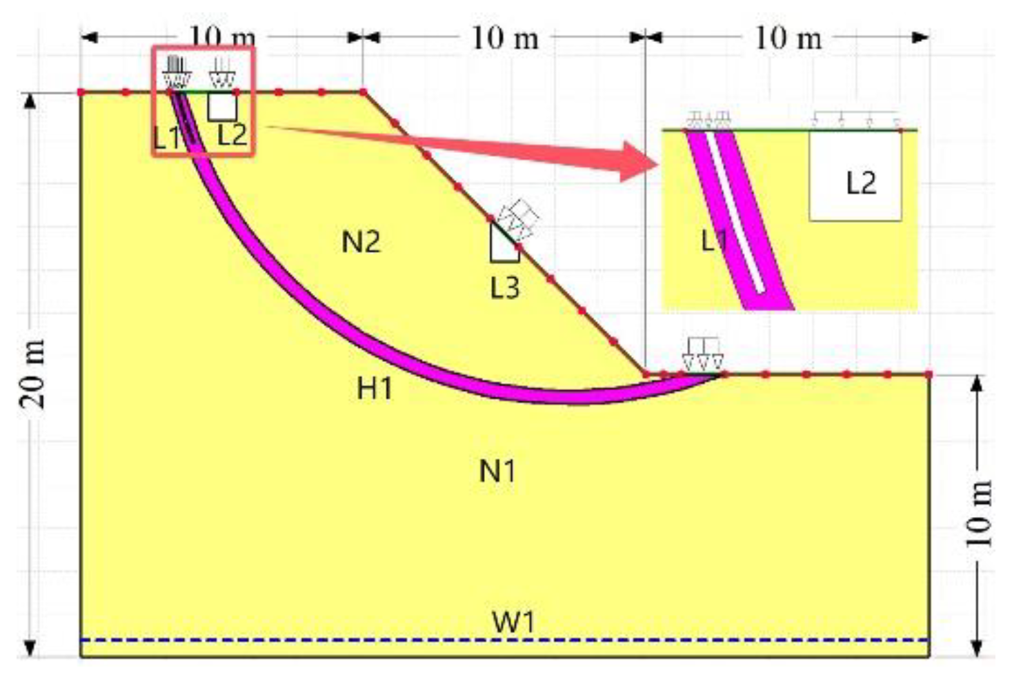
Figure 2.
Relationship curve between matric suction and volumetric water content of sliding soil.
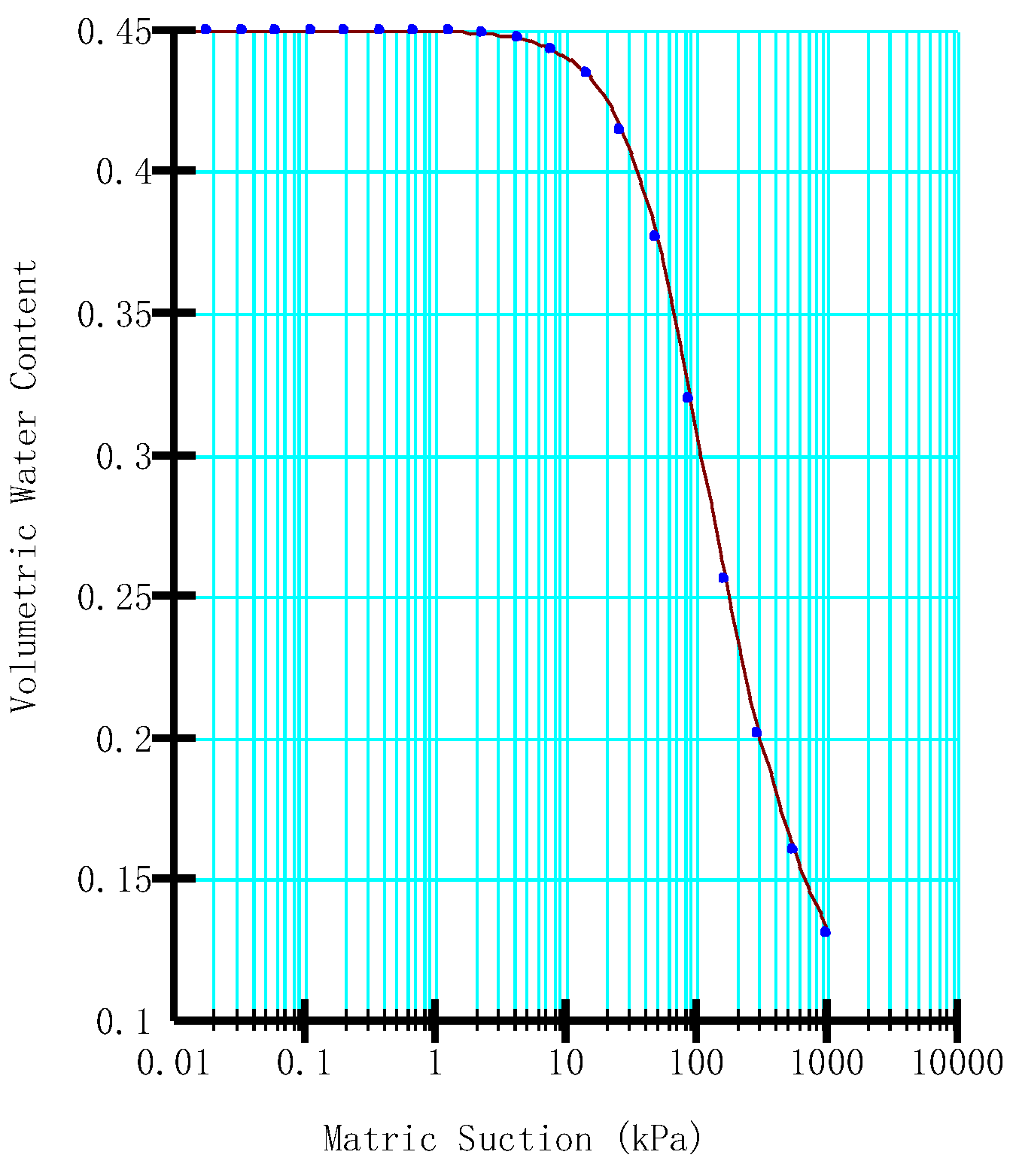
Figure 3.
Relationship curve between matric suction and water X-conductivity of sliding soil.
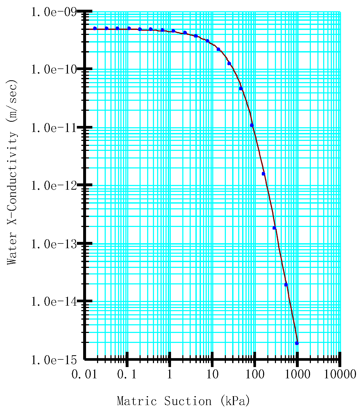
Figure 4.
Comparison between predicted values by XGBoost model and actual values.
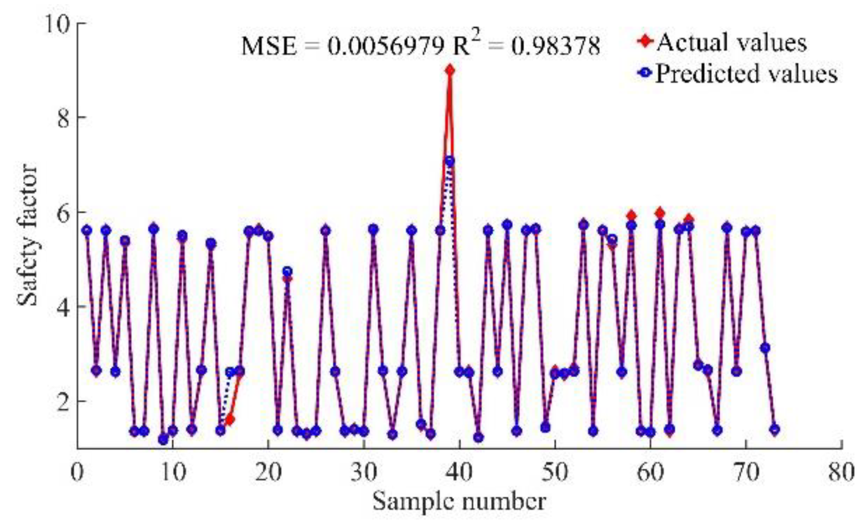
Figure 5.
Comparison between predicted values by PSO-SVR model and actual values.
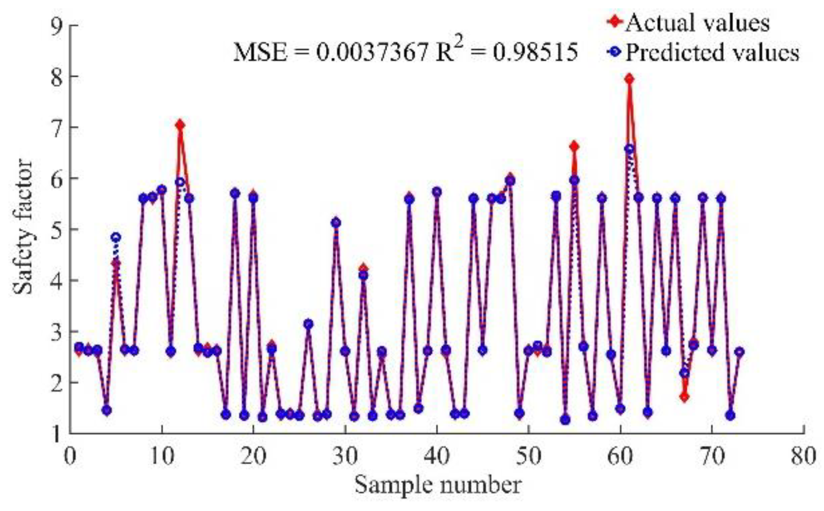
Figure 6.
Comparison between predicted values by XGBoost-PSO-SVR model and actual values.
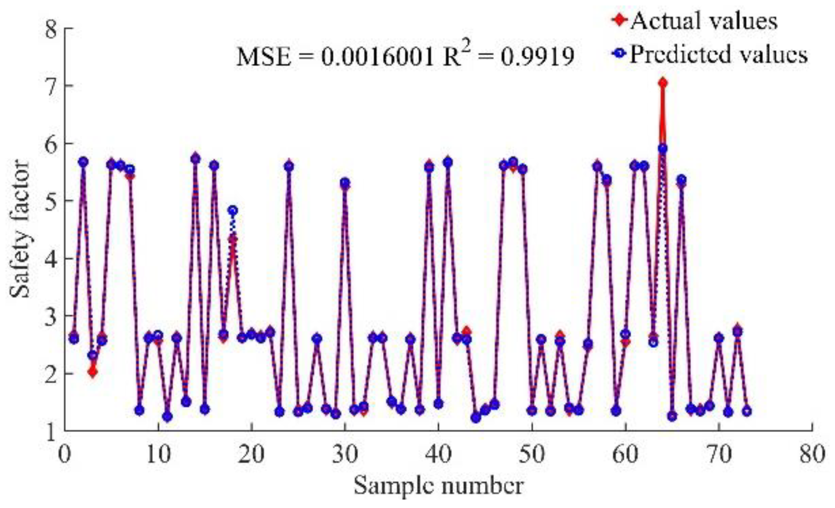
Figure 7.
Comparison between predicted values by four single-machine learning models and true values.
Figure 7.
Comparison between predicted values by four single-machine learning models and true values.
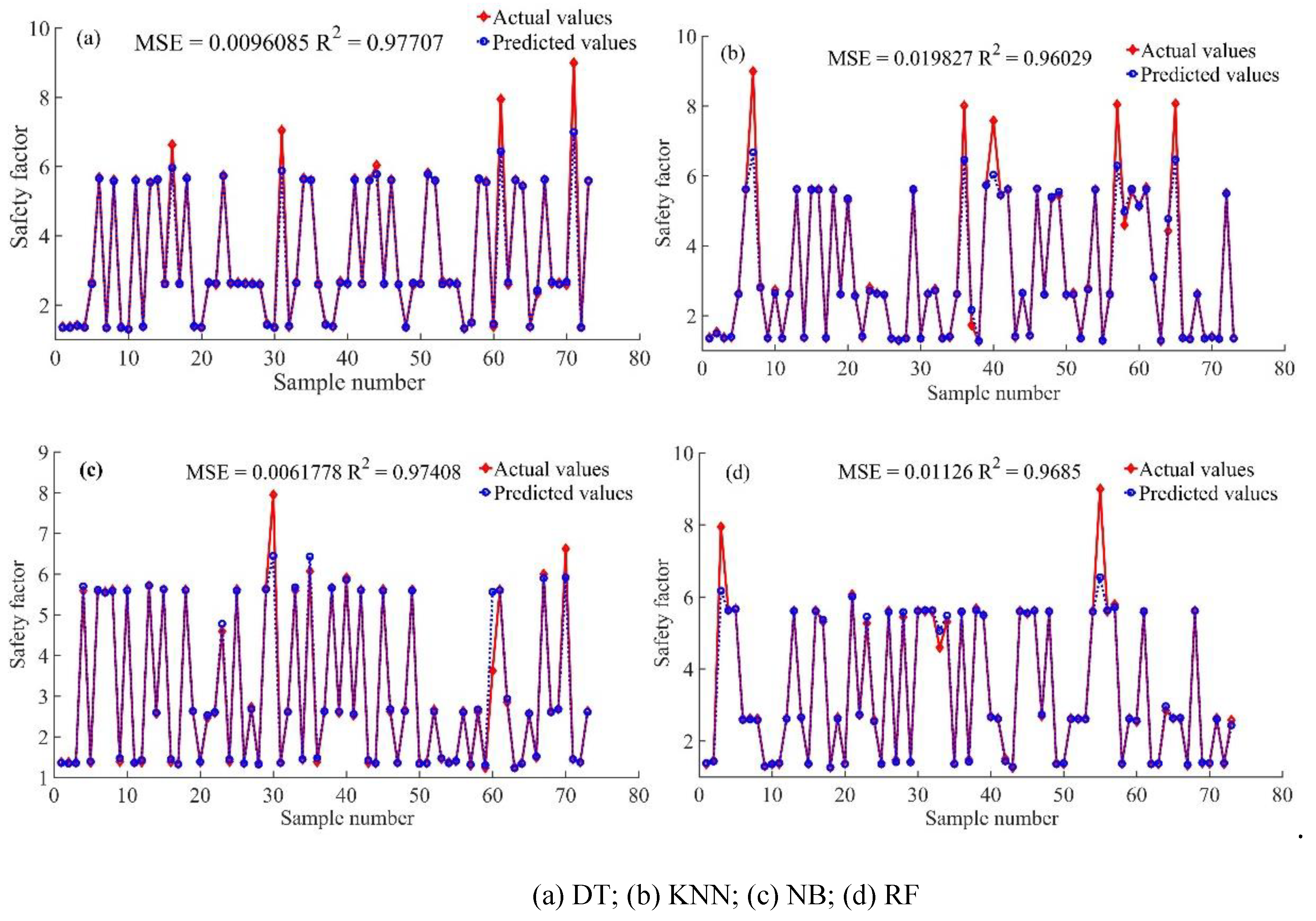
Figure 8.
Downward platforms at rear of a newly failed slope.
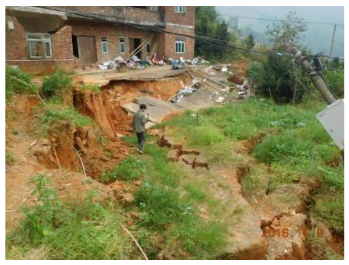
Figure 9.
A tensile crack at rear edge of the slope.
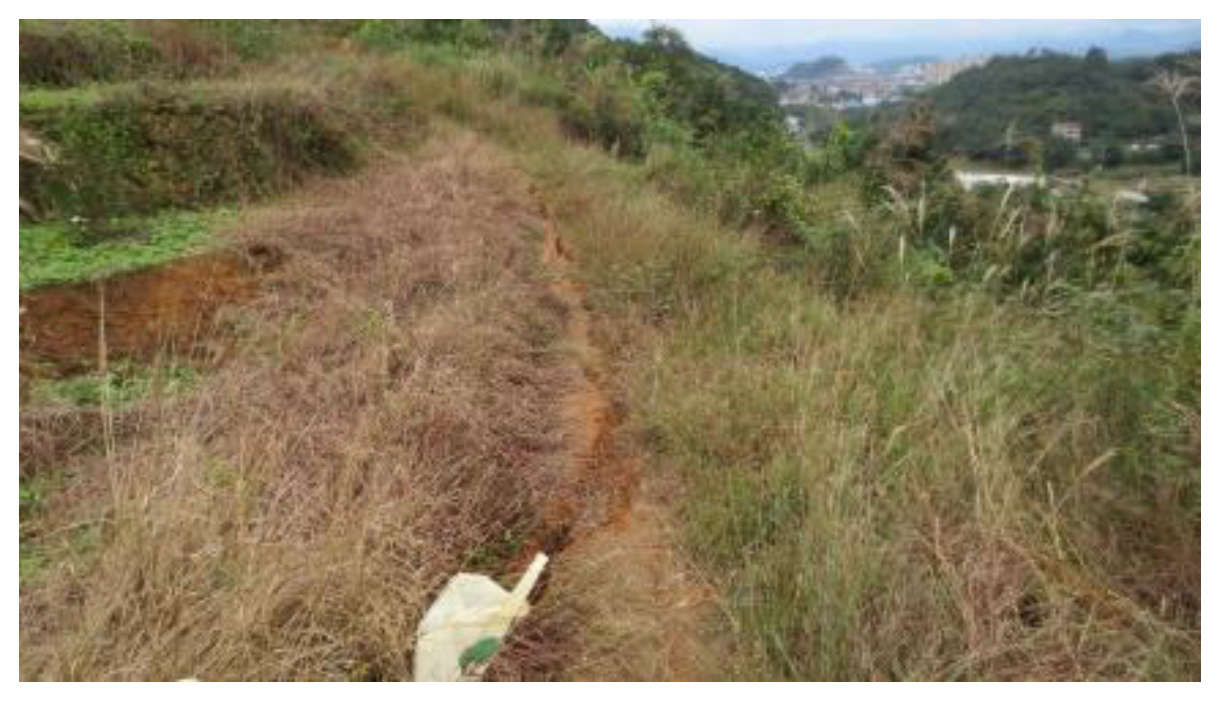
Figure 10.
The predicted results by XGBoost-PSO-SVR model.
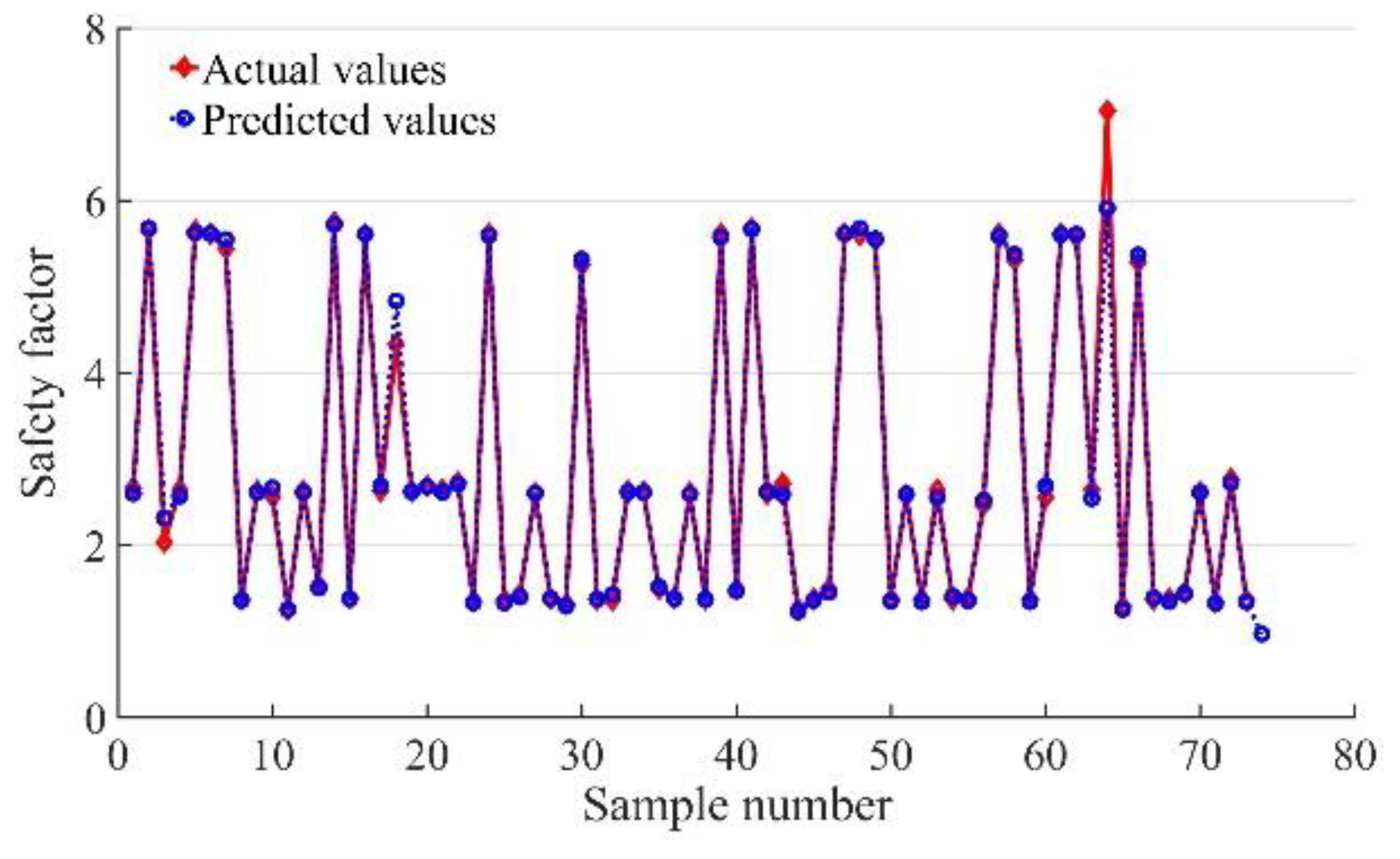

Table 1.
Numerical simulation grouping of each parameter.
| Group | H /m |
β /(︒) |
c /kPa |
φ /(︒) |
γ /(kN·m-3) |
Tr /d |
Ir /(mm·d-1) |
Dm /m |
Lm /m |
St /% |
Sf /% |
| Ⅰ | 5 | 22.5 | 79.5 | 17.25 | 17.0 | 1 | 10 | 0.05 | 1 | 5 | 5 |
| Ⅱ | 10 | 45 | 65 | 16.50 | 17.5 | 2 | 25 | 0.10 | 2 | 10 | 10 |
| Ⅲ | 15 | 67.5 | 50.5 | 15.75 | 18.0 | 3 | 50 | 0.15 | 3 | 15 | 15 |
Table 2.
Combination working conditions of various parameters in group Ⅱ.
| Combination |
H /m |
β /(︒) |
c /kPa |
φ /(︒) |
γ /(kN·m-3) |
Tr /d |
Ir /(mm·d-1) |
Dm /m |
Lm /m |
St /% |
Sf /% |
| 1 | 7.5 | 45 | 65 | 16.50 | 17.5 | 2 | 25 | 0.10 | 2 | 10 | 10 |
| 2 | 8.0 | 45 | 65 | 16.50 | 17.5 | 2 | 25 | 0.10 | 2 | 10 | 10 |
| 3 | 8.5 | 45 | 65 | 16.50 | 17.5 | 2 | 25 | 0.10 | 2 | 10 | 10 |
| 4 | 9.0 | 45 | 65 | 16.50 | 17.5 | 2 | 25 | 0.10 | 2 | 10 | 10 |
| 5 | 9.5 | 45 | 65 | 16.50 | 17.5 | 2 | 25 | 0.10 | 2 | 10 | 10 |
| 6 | 10.0 | 45 | 65 | 16.50 | 17.5 | 2 | 25 | 0.10 | 2 | 10 | 10 |
| 7 | 10.5 | 45 | 65 | 16.50 | 17.5 | 2 | 25 | 0.10 | 2 | 10 | 10 |
| 8 | 11.0 | 45 | 65 | 16.50 | 17.5 | 2 | 25 | 0.10 | 2 | 10 | 10 |
| 9 | 11.5 | 45 | 65 | 16.50 | 17.5 | 2 | 25 | 0.10 | 2 | 10 | 10 |
| 10 | 12.0 | 45 | 65 | 16.50 | 17.5 | 2 | 25 | 0.10 | 2 | 10 | 10 |
| 11 | 12.5 | 45 | 65 | 16.50 | 17.5 | 2 | 25 | 0.10 | 2 | 10 | 10 |
| 12 | 10.0 | 56.25 | 65 | 16.50 | 17.5 | 2 | 25 | 0.10 | 2 | 10 | 10 |
| ∙∙∙ | ∙∙∙ | ∙∙∙ | ∙∙∙ | ∙∙∙ | ∙∙∙ | ∙∙∙ | ∙∙∙ | ∙∙∙ | ∙∙∙ | ∙∙∙ | ∙∙∙ |
| 120 | 10.0 | 45 | 65 | 16.50 | 17.5 | 2 | 25 | 0.10 | 2 | 10 | 12 |
| 121 | 10.0 | 45 | 65 | 16.50 | 17.5 | 2 | 25 | 0.10 | 2 | 10 | 12.5 |
Table 3.
Numerical simulation results of each combination working condition in Group II.
| Combination | Safety factor | Combination | Safety factor | Combination | Safety factor |
| 1 | 3.120 | 12 | 2.783 | 23 | 2.461 |
| 2 | 2.993 | 13 | 2.726 | 24 | 2.495 |
| 3 | 2.843 | 14 | 2.688 | 25 | 2.528 |
| 4 | 2.847 | 15 | 2.654 | 26 | 2.562 |
| 5 | 2.803 | 16 | 2.641 | 27 | 2.595 |
| 6 | 2.629 | 17 | 2.629 | 28 | 2.629 |
| 7 | 2.459 | 18 | 2.612 | 29 | 2.662 |
| 8 | 2.341 | 19 | 2.602 | 30 | 2.695 |
| 9 | 2.030 | 20 | 2.594 | 31 | 2.728 |
| 10 | 1.867 | 21 | 2.586 | 32 | 2.761 |
| 11 | 1.724 | 22 | 2.579 | 33 | 2.793 |
Table 4.
Parameter values of XGBoost model.
| Parameter | Value | Parameter | Value |
| eta | 0.2 | subsample | 0.8 |
| min_child_weight | 1 | colsample_bytree | 0.8 |
| max_depth | 5 | colsample_bylevel | 1 |
| gamma | 0 | alpha | 1 |
| max_delta_step | 0 | scale_pos_weight | 1 |
Table 5.
Comparisons of safety factors prediction indicators by various models.
| Machine learning model | MSE | R2 |
| DT | 0.0096 | 0.9771 |
| KNN | 0.0198 | 0.9603 |
| NB | 0.0062 | 0.9741 |
| RF | 0.0113 | 0.9685 |
| XGBoost-PSO-SVR | 0.0016 | 0.9919 |
Table 6.
Parameter values for evaluating slope stability.
| Parameter | Value | Parameter | Value |
| H /m | 38 | Ir /(mm·d-1) | 31.525 |
| β/(︒) | 32.2 | Dm /m | 0.65 |
| c /kPa | 25 | Lm /m | 2.5 |
| φ/(︒) | 24 | St /% | 20 |
| γ/(kN·m-3) | 18.8 | Sf /% | 10 |
| Tr /d | 4 | - | - |
Table 7.
Comparisons of safety factors predicted by various models.
| Machine learning model | Predicted value | Stability state | Simulation results | Deviation |
| XGBoost-PSO-SVR | 0.966 | Unstable | 0.988 | 0.022 |
| XGBoost | 1.005 | Under stable | 0.017 | |
| PSO-SVR | 0.958 | Unstable | 0.030 | |
| DT | 1.009 | Under stable | 0.021 | |
| KNN | 0.955 | Unstable | 0.033 | |
| NB | 1.024 | Under stable | 0.036 | |
| RF | 1.017 | Under stable | 0.029 |
Disclaimer/Publisher’s Note: The statements, opinions and data contained in all publications are solely those of the individual author(s) and contributor(s) and not of MDPI and/or the editor(s). MDPI and/or the editor(s) disclaim responsibility for any injury to people or property resulting from any ideas, methods, instructions or products referred to in the content. |
© 2025 by the authors. Licensee MDPI, Basel, Switzerland. This article is an open access article distributed under the terms and conditions of the Creative Commons Attribution (CC BY) license (http://creativecommons.org/licenses/by/4.0/).
Copyright: This open access article is published under a Creative Commons CC BY 4.0 license, which permit the free download, distribution, and reuse, provided that the author and preprint are cited in any reuse.


