UAV Based Hyperspectral Imaging for PVY Detection: Machine Learning Insights

1. Introduction

Potato Virus Y (PVY) is a pathogenic virus within the Potyvirus genus and family Potyviridae [1] that is responsible for substantial losses in quality and yield in seed potatoes globally. The potato leaves may have mosaic patterns, deformations, leaf curling, and tuber necrosis depending on the strain and environmental conditions, if affected by the virus [2]. PVY is one of the most destructive pathogens in potatoes and causes economic yield losses up to 80% [3]. Though the global economic loss due to PVY is unknown at the moment, over $190 million has been reported as an annual loss in the European Union alone [4]. Thus, accurate and early detection of PVY is crucial for implementing timely management strategies to reduce economic loss and ensure food security.

The traditional approach to detecting the PVY virus includes serological assays and molecular techniques [5], such as Enzyme-Linked Immunosorbent Assay (ELISA) and Reverse Transcription Polymerase Chain Reaction (RT-PCR) [6]. While these methods are highly sensitive and specific, the process entails extensive labor, time, resource requirements, and susceptibility to human errors. The procedure involves picking leaves manually from the fields, and the virus being highly contagious [7], poses the risk of disease spread from vehicles or people walking through the field, potentially increasing pathogen spread. As agriculture moves toward precision farming, there is a growing demand for advanced, non-invasive, and high-throughput diagnostic technologies to address these limitations. Due to the increasing economic impact and need for non-invasive methods, remote sensing technologies have acquired significant attention in detecting the PVY virus. Remote sensing technologies offer efficient and non-invasive approaches for monitoring crop health and various disease infections including mosaic caused by PVY [8,9].

Remote sensing technologies utilizing multispectral and hyperspectral imaging (HSI) are pivotal in identifying physiological changes in plants that can indicate viral infections such as PVY [9]. These systems produce reflectance patterns that are correlated with the presence of PVY [10] and may allow early detection before visual symptoms manifest. Vegetation indices such as Normalized Difference Vegetation Index (NDVI) is derived from satellite imagery and researchers have found it useful to monitor crop health and growth [11,12]. The spectral signatures change with the growth stages of the crop and thus are useful for pre-symptomatic detections, significantly improving the timeliness of interventions and reducing the economic impact on yield losses.

HSI combines images and spectroscopy to provide spatial and detailed spectral information across a wide range of wavelengths, spanning from visible and near-infrared (Vis-NIR) (400-1000 nm) and shortwave infrared (SWIR) (1000-2500 nm) regions [13]. The detailed HSI spectral information is capable of capturing subtle changes in plant physiology caused by stress or disease. These changes may not be visible to the naked eye, however, they can manifest unique spectral signatures that can distinguish between healthy and infected plants. The advent of HSI in precision agriculture has wide varieties of applications, ranging from disease detection [14,15,16,17,18], weed identification[19,20,21], nutrient assessment [22,23,24,25,26], yield predictions [27,28,29,30] and soil characterization [31,32,33,34]. HSI can be integrated with UAVs for field-scale non-destructive sampling and real-time monitoring of PVY status [14]. The two biggest challenges with HSI processing are the calibration of the data using downwelling irradiacne to get the reflectance data and the high dimensionality of the HSI data as they typically consist of hundreds of spectral bands resulting in a ’data cube’ that requires advanced computational techniques to extract the meaningful information.

Advancements in machine learning (ML) and artificial intelligence have revolutionized the interpretation and capabilities of remote sensing for PVY detections. Deep learning (DL) techniques are applied to various image types such as hyperspectral, multispectral, and satellite images, achieving high classification accuracy in distinguishing healthy plants from PVY-infected potato plants [35,36]. ML and DL techniques excel at identifying patterns, reducing dimensionality, and building task-specific predictive models that make them suitable for precision agriculture applications. Commonly used ML-DL algorithms for HSI analysis include support vector machines (SVM) [37,38,39,40], random forests (RF) [41,42,43,44], and neural networks [38,41,45,46,47]. These algorithms can effectively handle high-dimensional HSI data while retaining most of the original information. Convolutional neural networks (CNNs) have particularly gained popularity in HSI analysis for their ability to extract hierarchical features as found in HSI data [45,46,47]. Labeled dataset is required for plant disease detections, and due to the expense and scarcity of such datasets unsupervised and semi-supervised learning approaches are gaining traction as viable alternatives.

While the integration of HSI and ML-DL has demonstrated considerable potential for PVY detections, several challenges remain. First, the spectral variability caused by environmental factors such as weather conditions, atmospheric illuminations, soil types and plant canopy structures will not assist in generalizing the learned models. Pre-processing techniques as discussed in Section 2.2.1 are essential for minimizing these effects and enhancing the quality of HSI data. Second, the high dimensionality of the HSI data is computationally expensive, particularly for large-scale applications. Commonly used dimensionality reduction techniques to address such issues are principal component analysis (PCA), linear discriminant analysis (LDA), and singular value decomposition (SVD) [48]. The choice of dimensionality reduction technique can significantly impact the performance of the training model. After careful evaluation, we decided to downsample the HSI data and use all the spectral bands. Third, the interpretability of ML-DL models remains a concern, especially for HSI data it is important to understand the most relevant spectral bands carrying the most valuable information for the specific tasks. We investigated various techniques and found only five small spectral regions of the HSI data carries the most relevant information as reported in Section 3.5. Nevertheless, the challenges in processing HSI data and model interpretation can be conquered, PVY detection using HSI remains relatively underexplored.

The integration of unmanned aerial vehicles (UAV) with mounted remote sensing tools has been instrumental in capturing high-resolution images and real-time monitoring of the potato fields [9]. Images collected with UAVs have high spatial resolutions and offer close-field assessments of crop health. The use of UAVs for PVY detection or any other precision agriculture management is ecological, enhances the reliability and efficiency of crop monitoring, and reduces the labor cost significantly for large-acre fields. The fusion of UAV-acquired images with machine learning and deep learning techniques has enhanced the scalability of these technologies and offers the potential to build customized systems for PVY detection using configurable integrated circuits. Producers can implement quick targeted management strategies in the infected areas of the field to reduce the spread of the virus and minimize economic loss.

Although there have been promising advancements in remote sensing techniques to detect PVY, challenges remain in the practical implementation of these systems in a real producer-field setting. Factors such as atmospheric conditions, lighting, variations in soil nutrients, moisture, crop canopy heterogeneity, and other confounding factors affect the remote sensing data. Furthermore, most of the research so far in detecting the PVY has collected their dataset in a greenhouse or lab environment by taking images of leaves or individual plants [10,49,50,51]. It thus does not simulate the real environmental conditions of an open field. The integration of UAV with hyperspectral camera distinguishes our work from the other relevant research, as we collected the dataset from an actual potato field out in the open, where all the environmental factors are a major concern. We hypothesize that the presence of PVY in producer fields can be detected using hyperspectral cameras integrated with UAVs. We also analyze and deduce the most relevant spectra that carry valuable information toward detecting PVY. This work is an extended report of our preliminary work based on hyperspectral remote sensing for PVY detection [14].

This research employs machine learning and deep learning techniques to detect the PVY virus in potato fields using hyperspectral cameras mounted on a UAV and identify the most relevant spectral bands in the visible and near-infrared spectra region. The paper is organized in a few sections. Section 2.1 details the experimental field and the hyperspectral dataset acquired using a UAV, Section 2.2 discusses the data processing and labeling procedures, Section 2.3 gives a bit of background on the machine learning and deep learning techniques used in this work followed by hyperparameter optimization approaches. The metrics used to evaluate the performance of the training models are explained in Section 2.4, followed by feature selection methods in Section 2.5 and the outline of the research in Section 2.6. The performance evaluation and comparisons are presented in Section 3. Finally, the paper is wrapped up with a discussion.

2. Materials and Methods

2.1. Field and Data

The experimental field was curated according to the need of this research and the status of individual plants was monitored. Hyperspectral data was collected using a visible and near-infrared (Vis-NIR) camera mounted on a drone suitable for remote sensing.

2.1.1. Experimental Field

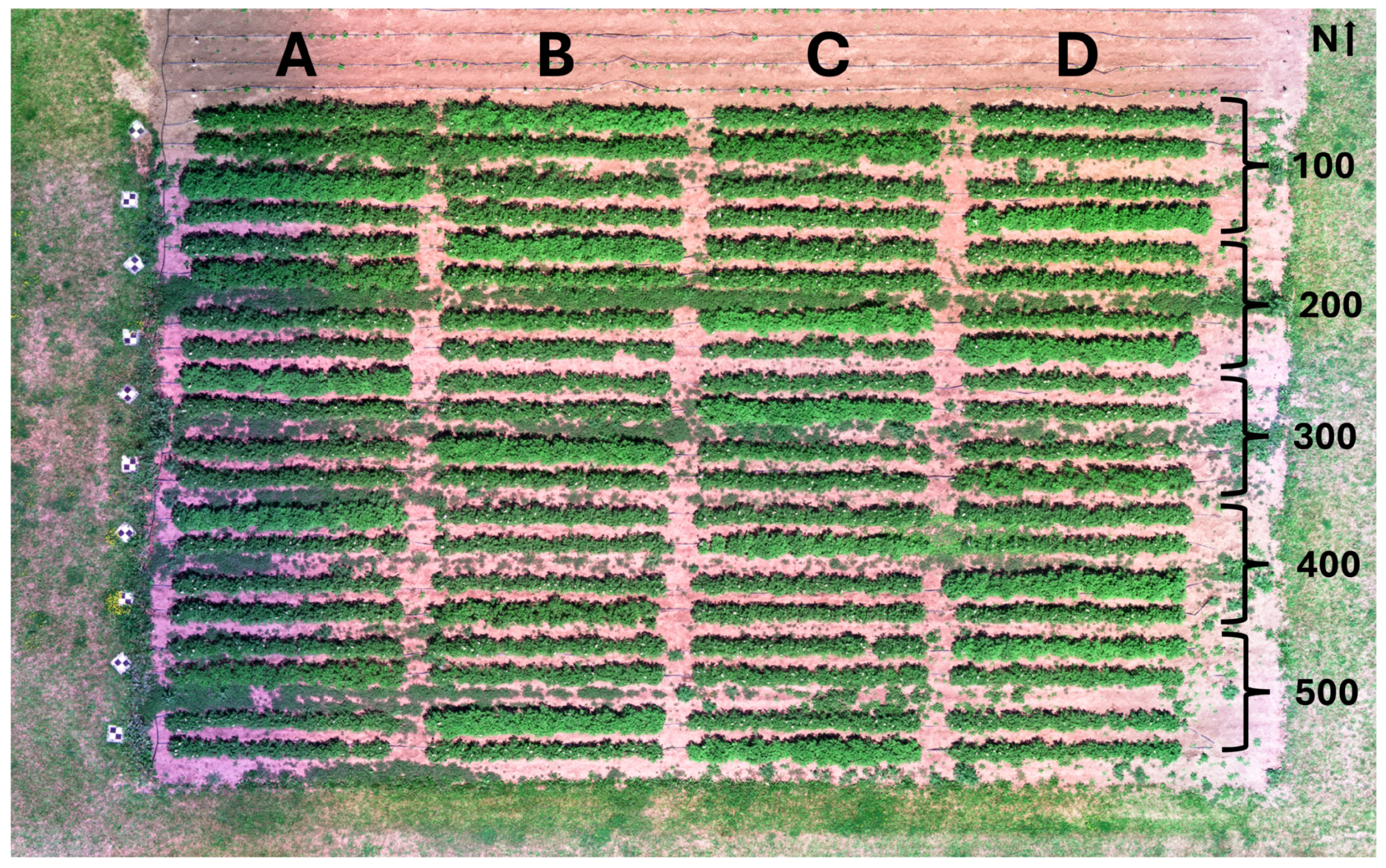
For research purposes, the experimental field, as shown in Figure 1, comprises multiple uniformly arranged plots for the PVY monitoring. Note that cloud shadow can be seen in the image, meaning the image is not downwelling irradiance corrected. We collected this mapped field using Micasense Altum-PT [52], a multi-spectral camera and used as a reference image of the field layout. The plots were planted at the Bozeman Agriculture Research and Teaching (BART) farm of Montana State University, Bozeman, MT. There are five blocks of potatoes with four rows in each of the blocks, four 20-foot plots with three feet of space, and 20 plants one foot apart. The plots were arranged to simulate family groups in generation one seed potatoes. To reduce the spread of the virus across the plots, the cultivars of potatoes in each row are as follows: one plot is experimental (susceptible to PVY), and the other three plots are Payette Russet potatoes (not susceptible to PVY). The Payette Russet variety is extremely resistant to different strains and genetic variants of PVY [53], which benefits us widely in reducing the spread of the virus and thus containing them to the desired plots.

Figure 1. Experimental field comprising of five blocks with four rows in each of the blocks. The five blocks are labeled as 100s to 500s, where they will be addressed as 101, 102, 103, high-spatial-resolution spectral data, and 104 for the four rows in the block #100. In each of the rows, one plot is susceptible to PVY, while the other three plots are resistant. The resistant cultivars are comparatively skinnier than the susceptible plots. For example, plot 101B is the experimental plot and is susceptible to PVY. Some ground control points with checkerboard patterns are placed along the west side of the field which helps in manually identifying the individual images captured by the camera.

Figure 1. Experimental field comprising of five blocks with four rows in each of the blocks. The five blocks are labeled as 100s to 500s, where they will be addressed as 101, 102, 103, high-spatial-resolution spectral data, and 104 for the four rows in the block #100. In each of the rows, one plot is susceptible to PVY, while the other three plots are resistant. The resistant cultivars are comparatively skinnier than the susceptible plots. For example, plot 101B is the experimental plot and is susceptible to PVY. Some ground control points with checkerboard patterns are placed along the west side of the field which helps in manually identifying the individual images captured by the camera.

Some of the susceptible plots were intentionally infected with PVY utilizing four different treatments to align with our research goal. In treatment one, the tubers testing positive by immunochromatography (IC) [54] were mixed 50:50 with Generation two of the Umatilla cultivar from Premiere Seed Potatoes PVY - in summer and winter. IC is a rapid diagnostic technique that utilizes antibodies binding to the target molecule to detect the presence of PVY virus in the tubers. In treatment two, the tubers testing negative by IC but from plants where sister tubers tested positive were planted. In treatment three, generation two Umatilla (UMA) cultivars from Premiere Seed Potatoes were planted. Finally, in treatment four, generation three Dark Red Norland (DRN) cultivars from Spring Creek Farms were planted. Table 1 furnishes the various treatments across the different experimental plots. The plots were tracked and later taken to the lab to perform the enzyme-linked immunosorbent assay (ELISA) test [55] to note the spread of the virus and create the ground truth for the dataset. Section 2.2.2 details about the ELISA test procedure. The Montana Seed Potato Lab was in charge of the experimental setup of the field and validating the in-season PVY status of each plant.

Table 1. Treatment descriptions across the field for all the five blocks of the experimental field. This is important to help facilitate the tracking of virus spread. T# represents the treatment used in the specific plots as mentioned in each of the rows.

Treatment	Block 100	Block 200	Block 300	Block 400	Block 500
T1 - 50% PVY	104 D	201 B	302 C	401 A	504 C
T2 - PVY+ Plants, PVY- Tubers	101 B	203 C	301 A	402 C	501 D
T3 - Uma Control	103 A	204 D	303 B	404 D	503 B
T4 - DRN Control	102 C	202 A	304 D	404 B	502 A

Table 1. Treatment descriptions across the field for all the five blocks of the experimental field. This is important to help facilitate the tracking of virus spread. T# represents the treatment used in the specific plots as mentioned in each of the rows.

Treatment	Block 100	Block 200	Block 300	Block 400	Block 500
T1 - 50% PVY	104 D	201 B	302 C	401 A	504 C
T2 - PVY+ Plants, PVY- Tubers	101 B	203 C	301 A	402 C	501 D
T3 - Uma Control	103 A	204 D	303 B	404 D	503 B
T4 - DRN Control	102 C	202 A	304 D	404 B	502 A

2.1.2. UAV and Hyperspectral Camera

Unmanned Aerial Vehicles (UAVs) or drones in general provide the ability to acquire high-spatial resolution spectral data which is a preferred tool in remote sensing. UAV systems enable disease surveys to be conducted without physically entering the field, thus reducing the risk of spreading the virus. For this project, we have used Vector Hexacopter [56] from Vision Aerial, equipped with the Resonon Pika L hyperspectral imaging camera [57], to capture high-resolution spectral data. The drone was flown at an altitude of 15 m above ground level (AGL) with a speed of 0.5 m/s to capture high-resolution images. Figure 2 shows a complete integration of the drone and the camera.

Figure 2. Resonon Pika L hyperspectral camera is mounted on the Vision Aerial Vector Hexacopter drone. A dual GPS/IMU and a downwelling irradiance sensor have been added for better GPS accuracy and to correct the reflection of lights in the captured images.

Figure 2. Resonon Pika L hyperspectral camera is mounted on the Vision Aerial Vector Hexacopter drone. A dual GPS/IMU and a downwelling irradiance sensor have been added for better GPS accuracy and to correct the reflection of lights in the captured images.

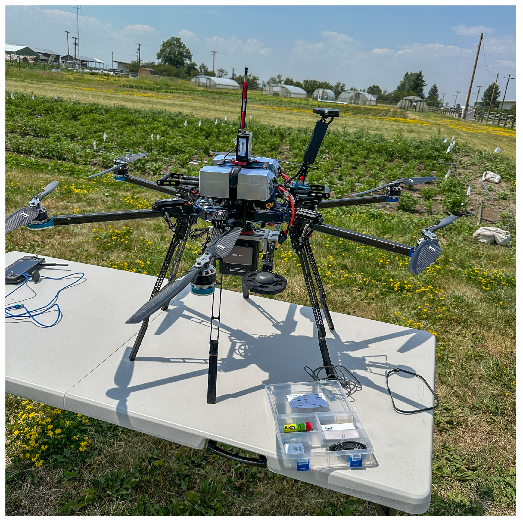
Vector Hexacopter UAV: Vector Hexacopter is an American-made industrial drone designed for longer-range missions and heavy lifting with a maximum payload capacity of 11 lbs. The drone can run for around 30 minutes with the camera attached, and the batteries can be hot-swapped if needed. The drone has six rotors and is powered by two 22000 mAh solid-state Li-ion batteries. The GPS accuracy of the drone is typically less than $\pm 1m$, however can vary up to $\pm 2.5m$. The software of the drone provides loitering that holds the position of the drone at any given moment in manual mode if the pilot does not provide any flight instructions. Mission plans are useful for autonomous flights, and brake mode, return to launch, low-battery protection, and lost link protection are some of the features that are available with the drone software.

Resonon Pika L Hyperspectral Camera: Resonon Pika L is a compact, lightweight Vis-NIR hyperspectral camera capturing 281 spectral channels across 400 - 1000 nm. The camera provides a spectral resolution of 2.7 nm with 900 spatial pixels. We have used a 17 mm focal length camera with a 17.6 degrees field of view. For better GPS accuracy an Ellipse 3D dual-antenna GPS/IMU has been added on, and to correct the light reflection of the images, a downwelling irradiance sensor has been used as well. Spectronon [58] is a free software provided by Resonon that helps in hyperspectral data acquisition and analysis.

2.1.3. Hyperspectral Dataset

The data used in this experiment were collected on July 12th, 2023 within one hour of the solar noon at the Montana State University BART farm. The Resonon Pika L hyperspectral camera generates datacubes of 2000 line scans with 900 pixels and 300 spectral channels. Note that, some of the spectral channel data are very noisy and do not contain any meaningful information, and thus need to be discarded. Unfortunately, our magnetometer of the camera failed and the data could not be geo-rectified and stitched together. Thus, we had to manually arrange the images with the help of the image orientation and the ground control points with the checkerboard patterns, to create the field layout as seen in Figure 3. A Micasense Altum-PT multispectral camera [52] mounted on a DJI Matric 600 [59] UAV, was flown five days later over the same field to create the reference image for the manual rectification and arrangement of the hyperspectral images. The geo-rectified and orthomosaic image of the field which has been used as the reference image is shown in Figure 1.

Figure 3. The relevant hyperspectral images were manually put together to recreate the field layout [14]. Due to the technical failure in the magnetometer of the camera, the images could not be geo-rectified. Hence, for the manual arrangement of the field layout, the images needed to be flipped and rotated to match the original layout of the field and account for the flight direction. The block numbers starting from 101-504 and the rows plots A, B, C, and D are labeled for reference. The numbers in green on both sides of the figure represent the image numbers, and the letter F and R stands for flipped and rotated. A calibration tarp can be seen in a few of the images, however, we have used downwelling irradiance sensor data for reflectance calibration of the images.

Figure 3. The relevant hyperspectral images were manually put together to recreate the field layout [14]. Due to the technical failure in the magnetometer of the camera, the images could not be geo-rectified. Hence, for the manual arrangement of the field layout, the images needed to be flipped and rotated to match the original layout of the field and account for the flight direction. The block numbers starting from 101-504 and the rows plots A, B, C, and D are labeled for reference. The numbers in green on both sides of the figure represent the image numbers, and the letter F and R stands for flipped and rotated. A calibration tarp can be seen in a few of the images, however, we have used downwelling irradiance sensor data for reflectance calibration of the images.

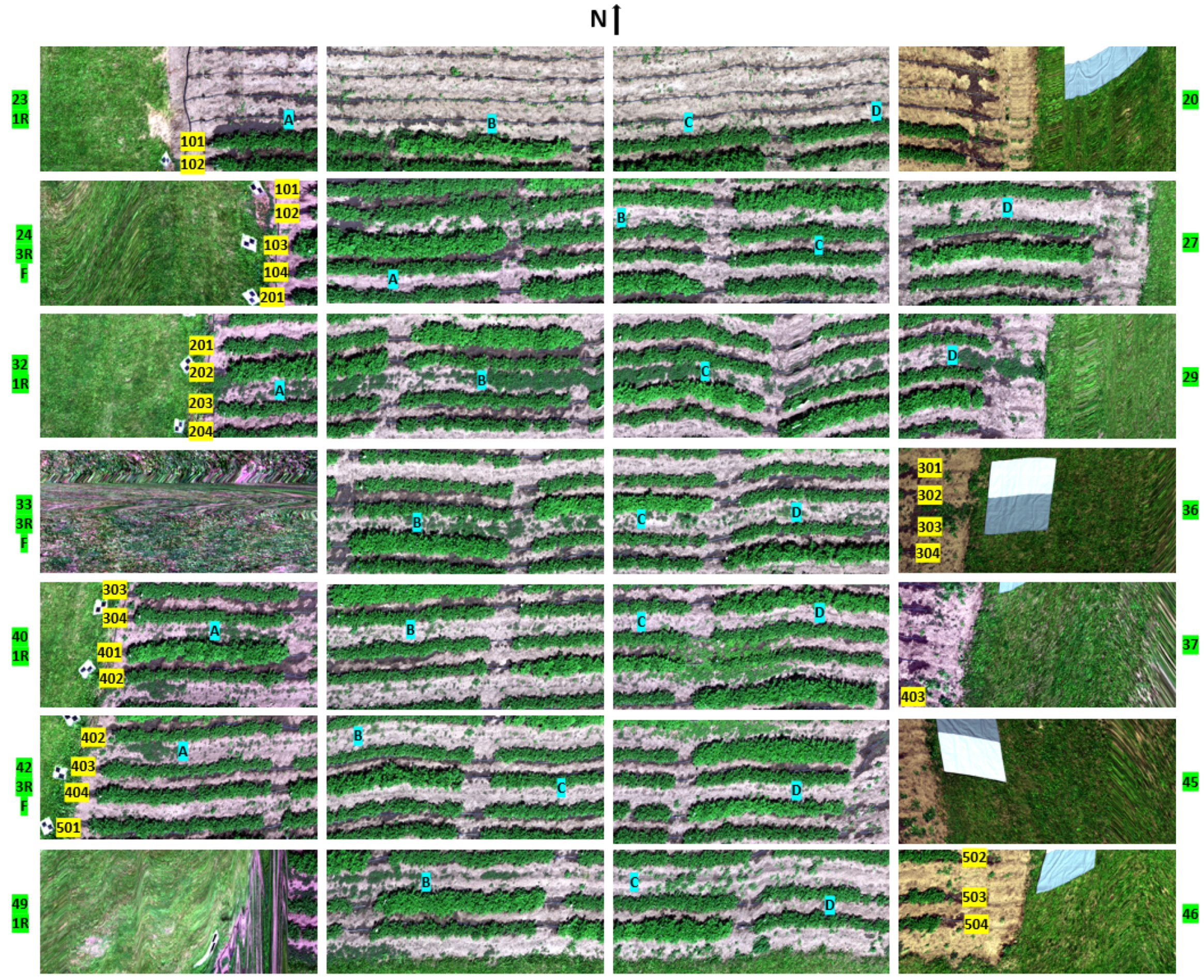
Some of the images in Figure 3 are wobbly as the drone appeared to be unstable at lower altitude flights and at a slower speed, and the issue with the IMU magnetometer prevented correction via geo-rectification. We flew the drone at 15 m AGL and 0.5 m/s as the field was comparatively smaller and we were interested in high-resolution images; however, a flight with $\ge 50m$ AGL and $3-5m/s$ speed would make the drone more stable and produce steady images. Upon investigating the collected hyperspectral images, we found 19 images with susceptible plots in them contained meaningful data and we have used those images for this experiment. Each of the images contains 2000 x 900 = 1800000 pixels. 15 images (around 80%) were used for training and validation of the machine learning models and the rest four images were used for testing the trained models.

2.2. Data Processing

The hyperspectral data captured via the Resonon Pika L camera were preprocessed utilizing the hyperspectral analysis software, Spectronon [58]. These preprocessing steps are crucial to ensure accurate and meaningful analysis.

2.2.1. Preprocessing

Figure 4 illustrates a flowchart of the necessary preprocessing steps taken to prepare the raw data for ML-DL analysis. The steps include radiometric calibration, reflectance calibration, smoothing, bad band removals, normalization, NDVI and downsampling.

Figure 4. Steps followed in this work to process the raw data before Ml-DL analysis.

Figure 4. Steps followed in this work to process the raw data before Ml-DL analysis.

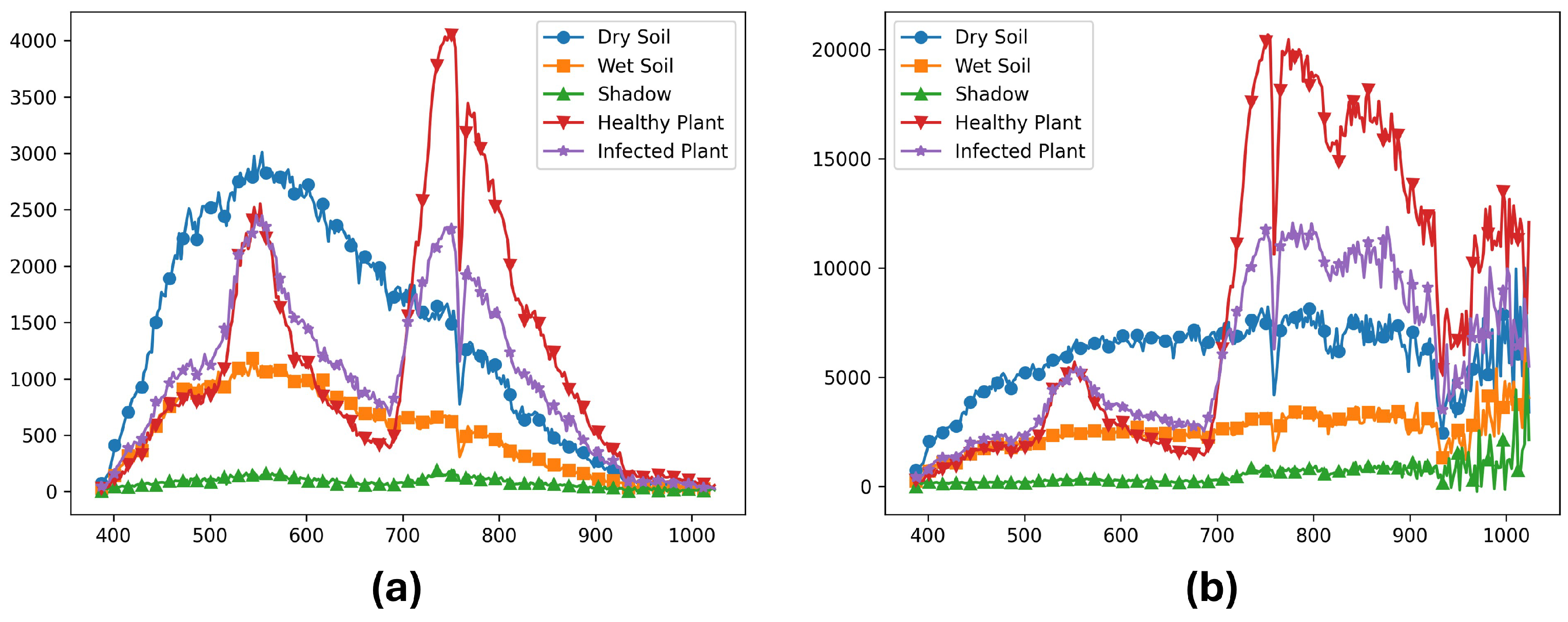
Raw Data: The raw data is uncalibrated and represented as digital numbers. This data can not be compared with data from a different instrument or illumination conditions until they are corrected to account for those differences. Figure 5(a) shows an RGB (red, green, blue) representation of a sample image of the raw data. The sample image comprises healthy and infected plants, resistant varieties, background soil, and the plants from the susceptible plots which could not be isolated due to GPS uncertainty. These non-isolated plants are labeled as unknown, as shown in Figure 5(c). The spectra of this image look very different for each of the classes as seen in Figure 6(a). The plant foliage and dry soil have high peaks in the visible spectrum, and the healthy plants exhibit high peaks in the red-edge region (680 - 750 nm), which is typical for vegetation. The infected plants also show a similar pattern, however, they are less pronounced in the near-infrared (NIR) region (> 700 nm). Shadow is almost a flat line due to the absence of illumination, and the wet soil reflects similarly to dry soil, but with a lower intensity due to water absorption.

Radiance Data: Radiance data refers to the amount of electromagnetic energy emitted or reflected from a surface per unit area and solid angle [60]. Radiance depends on the direction and intensity of the illumination. The data also changes with atmospheric effects such as scattering, absorption, etc. Radiance data for any wavelengths, $\lambda$ can be obtained from the raw data (digital numbers, $DN\left(\lambda \right)$) using Equation 1.

$$L\left(\lambda \right)={\displaystyle \frac{DN\left(\lambda \right)-D{N}_{\mathrm{dark}}}{C\left(\lambda \right)\times \Delta e}}$$

(1)

where, $L\left(\lambda \right)$ is the radiance, $D{N}_{\mathrm{dark}}$ is the dark correction signal of the hyperspectral sensor, $C\left(\lambda \right)$ is the radiometric calibration coefficient of the hyperspectral sensor, and $\Delta e$ is the exposure time of the sensor. Figure 6(b) shows the radiance calibration of all the categories. The plants vs soils became distinct after radiance calibration. Wet soil is consistent with the dry soils, but with a lower intensity, and shadows are flat with minimal reflectance across all wavelengths. Healthy plants show strong intensity at the red-edge bands and high NIR reflectance due to chlorophyll. The infected plants exhibit a similar pattern but with reduced reflectance, indicating physiological stress.

Figure 5. True color (red: 639.8 nm, green: 550.00 nm, blue: 459.7 nm) representation of the (a) raw data, (b) processed data for a sample hyperspectral image, and (c) the respective ground truth labels of the image. The raw data is captured by the camera, and the processed data is radiance and reflectance calibrated, and finally normalized. The label contains background; healthy and infected plants - these plots are susceptible to PVY; resistant - these plots are resistant to PVY; and the unknown labels meaning the unknown status of PVY.

Figure 5. True color (red: 639.8 nm, green: 550.00 nm, blue: 459.7 nm) representation of the (a) raw data, (b) processed data for a sample hyperspectral image, and (c) the respective ground truth labels of the image. The raw data is captured by the camera, and the processed data is radiance and reflectance calibrated, and finally normalized. The label contains background; healthy and infected plants - these plots are susceptible to PVY; resistant - these plots are resistant to PVY; and the unknown labels meaning the unknown status of PVY.

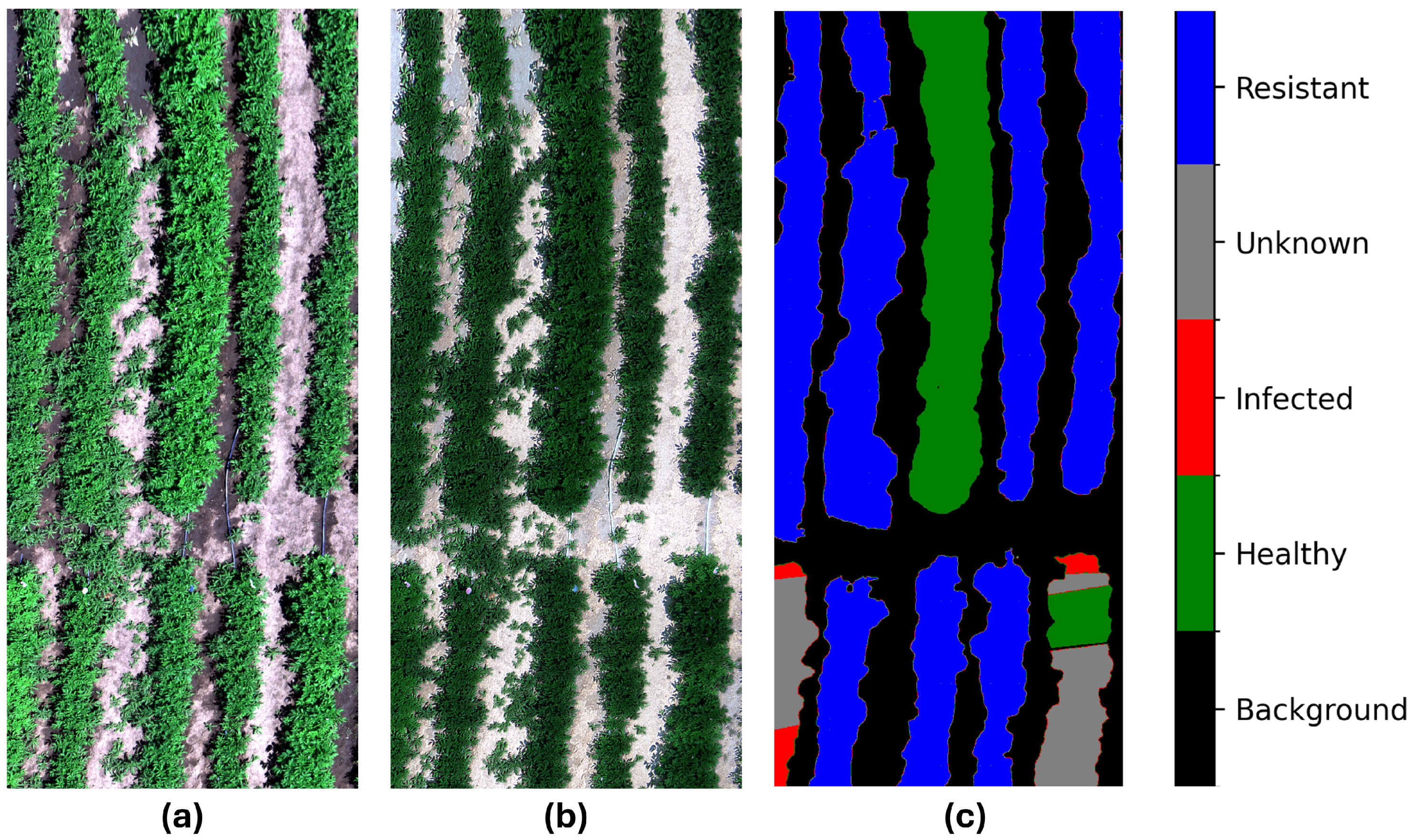
Figure 6. (a) Raw data and (b) Radiance calibrated data for dry soil, wet soil, shadow, healthy plant, and infected plant from the same sample image. The x-axis represents the wavelengths in nanometers, and the y-axis represents (a) digital numbers (DN) produced by the camera, and (b) physical units of microFlicks ($W/m^2.sr.nm$) (power per unit solid angle per unit area).

Figure 6. (a) Raw data and (b) Radiance calibrated data for dry soil, wet soil, shadow, healthy plant, and infected plant from the same sample image. The x-axis represents the wavelengths in nanometers, and the y-axis represents (a) digital numbers (DN) produced by the camera, and (b) physical units of microFlicks ($W/m^2.sr.nm$) (power per unit solid angle per unit area).

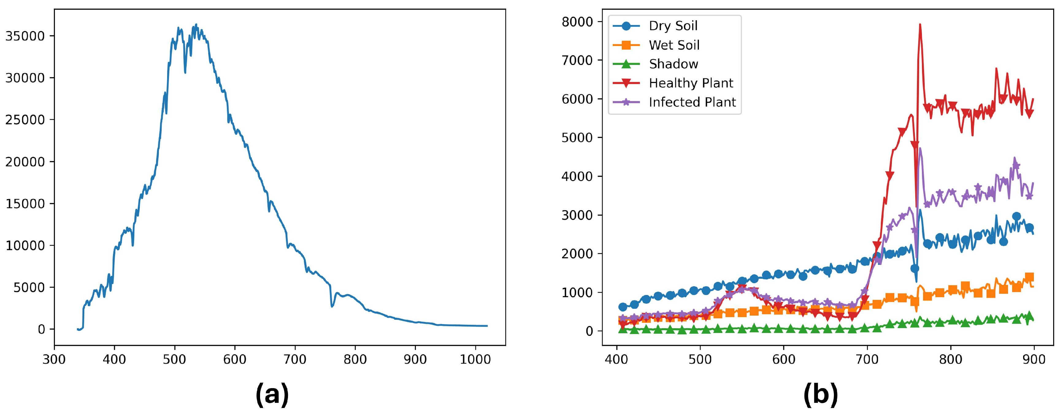
Reflectance Data: Reflectance is the ratio of the light that leaves a target to the amount of light that hits the target [61]. It is dimensionless and has no units. To calculate reflectance we need the downwelling spectral irradiance or downwelling irradiance in short, which is the amount of solar illumination reaching the ground. Figure 7(a) shows the amount of illumination that reached the ground during the time of flight, captured by a downwelling sensor mounted on the UAV and the hyperspectral camera. Let $I\left(\lambda \right)$ be the downwelling irradiance, then reflectance $R\left(\lambda \right)$ is:

$$R\left(\lambda \right)={\displaystyle \frac{\pi \times L\left(\lambda \right)}{I\left(\lambda \right)}}$$

(2)

Reflectance calibration is crucial because it allows data comparison captured at different times or with different sensors. Figure 7(b) shows the calibrated reflectance measurements for different categories. Absorption occurs at around 747 nm - 770 nm, and thus we see sudden changes in the reflectance. Shadow is as usual a flat line with almost no reflectance. We can notice distinct contrasts between dry soil and wet soil due to water absorption differences. Though both healthy and infected plants show similar spectra across the visible range, they differ in the NIR region, and the reduced pronunciation indicates the stress or infections in the plant.

Figure 7. (a) Downwelling spectra used for reflectance calibration, and (b) Reflectance calibrated data for dry soil, wet soil, shadow, healthy plant, and infected plant from the same sample image. The x-axis represents the wavelengths in nanometers, and the y-axis represents (a) downwelling irradiance physical units $W/m^2/nm$, and (b) the unitless ratio of reflectance value.

Figure 7. (a) Downwelling spectra used for reflectance calibration, and (b) Reflectance calibrated data for dry soil, wet soil, shadow, healthy plant, and infected plant from the same sample image. The x-axis represents the wavelengths in nanometers, and the y-axis represents (a) downwelling irradiance physical units $W/m^2/nm$, and (b) the unitless ratio of reflectance value.

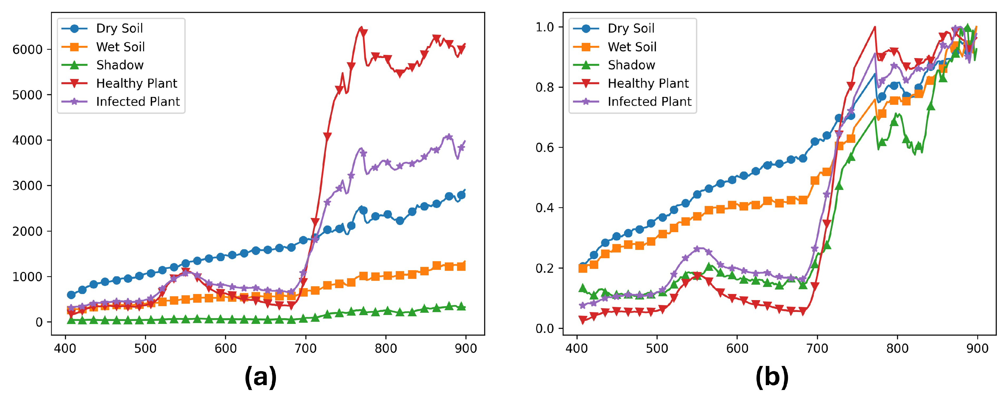
Savitzky-Golay Smoothing: To reduce the noise in the reflectance data, a Savitzky-Golay filter was fitted through the data with a 3rd-degree polynomial and 13-point slider window for the polynomial fitting by the method of linear least squares [62]. This is a widely used filter to smooth the hyperspectral data while preserving the vital spectral features. Smoothed reflectance data using the Savitzky-Golay filter can be obtained as follows:

$$R_{\mathrm{smoothed}}\left(\lambda \right)=\sum _{j=-w}^w{c}_j·R_{\lambda +j}$$

(3)

where, $R_{\mathrm{smoothed}}\left(\lambda \right)$ is the smoothed reflectance, $c_j$ are the polynomial coefficients, and w is half of the sliding window size. Figure 8(a) shows the smoothed reflectance data for all the categories. The noise is reduced in the data and looks smoother, however, the key spectral features are preserved.

Figure 8. (a) Smoothed reflectance data using Savitzky-Golay filter and (b) Normalized reflectance data for dry soil wet soil, shadow, healthy plant, and infected plant from the same sample image. Note the bad bands are discarded in the plots. The x-axis represents the wavelengths in nanometers and the y-axis represents (a) the unitless ratio of reflectance values, and (b) the normalized reflectances ranging from 0 to 1.

Figure 8. (a) Smoothed reflectance data using Savitzky-Golay filter and (b) Normalized reflectance data for dry soil wet soil, shadow, healthy plant, and infected plant from the same sample image. Note the bad bands are discarded in the plots. The x-axis represents the wavelengths in nanometers and the y-axis represents (a) the unitless ratio of reflectance values, and (b) the normalized reflectances ranging from 0 to 1.

Bad Band Removal: The hyperspectral sensor gives 300 spectral channels from 387.12 nm to 1023.5 nm. Some of the spectra in the beginning and the end are extremely noisy and do not contain any meaningful information. If the spectra are represented by band numbers 0-299, we cropped the wavelengths and kept 10-243 to remove the noisy spectra in the beginning and the ending. Due to absorption, we have also removed a few spectra (747 - 770 nm) from the red edge bands. Finally, we ended up with 223 spectral channels for the experiment.

Normalization: We normalized the data using the maximum method, where each pixel in the image is divided by the maximum intensity across all the wavelengths in that pixel. The values are then scaled to a range from 0 - 1, effectively reducing the variabilities for measurement conditions, and improving the machine learning analysis. Figure 8(b) shows the normalized reflectance spectra for a few selected pixels of the sample image. The spectral features that arise in the normalized shadow data are due to the diffuse illumination reflecting from the plant leaves leading to spectra that are similar to a plant but with much lower intensity. Figure 5(b) shows the true color representation of the sample image after completing all the preprocessing steps (raw data to normalized data).

NDVI and Downsampling: We calculated the Normalized Difference Vegetation Index (NDVI) of the images, which mostly measures the photosynthetic activities of the plants to get the vegetation [63] and potentially remove any unwanted objects from the images. NDVI is calculated from the red band and the NIR band.

$$NDVI={\displaystyle \frac{NIR-Red}{NIR+Red}}$$

(4)

We have also downsampled the images to imitate flying at a higher AGL and reduce the computational complexity of machine learning model training. If an image is $I(x,y)$, we first do a convolution with a kernel of size $k\times k$, then subsample every k-th element to downsample. For the hyperspectral cube, the third dimension or the spectral bands were not downsampled.

$$\begin{array}{c}\hfill I_{\mathrm{conv}}(x,y)=\sum _{i=0}^{k-1}\sum _{j=0}^{k-1}I(x+I,y+j)\\ \hfill I_{\mathrm{downsampled}}(x^{\prime },y^{\prime })=I_{\mathrm{conv}}(k{x}^{\prime },k{y}^{\prime })\end{array}$$

(5)

2.2.2. ELISA Test

ELISA (Enzyme-Linked Immunosorbent Assay) was performed for all the plants individually to track their PVY status. ELISA is a qualitative serological assay for the detection of PVY [55,64,65] in potato leaves. The leaf samples were collected from the field and the location of the plants in the plot was recorded. The leaf samples were then extracted in pressing trays 4000 psi using a drill press in a blotto buffer solution containing sodium azide as a preservative. This solution dilutes the enzyme conjugate to add to the immunocapture plates that had been prepared earlier. These plates are coated with IgG antibodies and blocked to prevent non-specific binding. The samples added to the plates are then incubated overnight at $4^{\circ }$C. The plates are then washed 4x with PBS (phosphate buffer saline) Tween and enzyme-conjugated antibodies are added. The plates are then incubated again at ${37}^{\circ }$C for 1-4 hours followed by another 3x wash in PBS Tween. P-nitrophenyl phosphate substrate is added and the plates are read when the controls have a suitable color (30-60’). This method ensures the detection of PVY and is crucial to creating the ground truth labels of our dataset.

2.2.3. Labeling

We have labeled the hyperspectral images to pixel levels using the ELISA test results as the ground truth reference. The dataset was labeled in a sem-manual manner using the Computer Vision Annotation Tool (CVAT) [66] platform to the background, infected, not infected, resistant, and unknown classes. A sample of the labeled data is shown in Figure 5(c). Note, the images in Figure 3 were labeled, taking Figure 1 as the reference layout of the field.

2.3. Machine Learning and Deep Learning

The hyperspectral dataset was trained and assessed using several machine learning (ML) methods, ranging from traditional algorithms to advanced deep leaning (DL) approaches. Below, we discuss the models used: Support Vector Machine (SVM), Decision Tree, k-Nearest Neighbors (KNN), Logistic Regression, Neural Network (NN), and Convolutional Neural Network (CNN).

2.3.1. Support Vector Machine

Support Vector Machine (SVM) is a supervised learning algorithm that finds the hyperplane that best separates the data into different classes leveraging the support vectors in the N-dimensional space [67]. The support vectors are the closest data points that maximize the class boundaries and define the hyperplane. Suppose we have a training dataset ${\left\{(x_i,y_i)\right\}}_{i=1}^n$, where $x_i\in {\mathbb{R}}^d$ are the features and $y_i\in \{-1,1\}$ are the labels, then the optimal margin can be obtained by minimizing:

$$\begin{array}{cc}\hfill \underset{w,b}{min}& {\displaystyle \frac{1}{2}}{\left|\right|w\left|\right|}^2\hfill \\ \hfill \mathrm{s}.\mathrm{t}.& y_i(w^{\mathrm{T}}{x}_i+b)\ge 1\hfill \end{array}$$

(6)

where, w is the weight vector and b is the bias. The decision function for a new input x will be:

$$f\left(x\right)=\mathrm{sign}(w^{\mathrm{T}}x+b)$$

(7)

For non-linear classification, kernel functions $K(x_i,x_j)$ can map the input features into higher-dimensional spaces. Some common kernels are linear kernel: $x_i^{\mathrm{T}}{x}_j$; polynomial kernel: ${(x_i^{\mathrm{T}}{x}_j+c)}^d$, where $c\ge 0$ is a free parameter to trade off the influence of higher order polynomial and d is the degree of the polynomial; and radial basis function kernel: $exp(-\gamma ||x_i-x_j|{|}^2$ etc.

2.3.2. Decision Tree

A decision tree is a non-parametric supervised learning algorithm that has a hierarchical tree-like structure partitioning the feature space into subsets based on feature values, aiming to minimize the impurities of target variables within each subset. There are two main scoring criteria Information Gain and Gini Index [68]. If the probability of class k in a node q is $p_k$, then information F can be calculated as:

$$F=-\sum _k{p}_k{\log }_2{p}_k$$

(8)

Information gain, $\Gamma$ for the jth subspace is calculated as:

$$\Gamma =F\left(\mathrm{parent}\right)-\sum _j{p}_{j}F\left({\mathrm{child}}_j\right)$$

(9)

The Gini Index, $GI$ measures the impurities in the class nodes and can be calculated from Equation 10.

$$\begin{array}{c}\hfill \mathrm{impurity},ϵ=1-\sum _k\left|\right|p\left(k\right)N_k\left(q\right)/N_k{\left|\right|}^2\\ \hfill GI=ϵ\left(\mathrm{parent}\right)-\sum _j\left(p_j\right)ϵ\left({\mathrm{child}}_j\right)\end{array}$$

(10)

here, $p_k=N_k/N\left(1\right)$ is the prior probability that a sample belongs to class k and $N_k\left(q\right)$ is the number of class k samples in node q.

2.3.3. k-Nearest Neighbors

K-nearest neighbors (KNN) is a non-parametric supervised learning algorithm that assigns a new data point based on the majority class among its k nearest neighbors [69]. First, the distance is computed between the target data point and all the points in the training data. Euclidean distance is a widely used metric for computing the distance.

$$d(x_m,x_n)=\sqrt{{\sum }_{p=1}^q{(x_{mp}-x_{np})}^2}$$

(11)

Next, the k nearest neighbors are identified based on the distances, d. Finally, the class label is assigned based on the majority set of the k-nearest neighbors.

2.3.4. Logistic Regression

Logistic regression is a statistical model that uses logistic functions to represent the binary outcome of an event [70]. For an input vector $x\in {\mathbb{R}}^d$, weight vector w, and the bias b, the probability of the positive class is:

$$P(y=1|x)={\displaystyle \frac{1}{1+e^{-(w^{\mathrm{T}}x+b)}}}$$

(12)

Instead of minimizing the loss, we can maximize the (positive) log-likelihood $\mathcal{L}(w,b)$ to estimate w and b.

$$\mathcal{L}(w,b)=\sum _{j=1}^k{y}_j\log \left(P\left(y_j\right)\right)+(1-y_j)\log (1-P\left(y_j\right))$$

(13)

2.3.5. Neural Network

Neural networks (NN) are computational models that are highly effective for learning non-linear patterns in data. This method algorithm uses interconnected neurons, called nodes, inspired by human brains [71]. A basic NN consists of three layers: an input layer that takes the input features ($x\in {\mathbb{R}}^d$); one or more hidden layers - the layer of artificial neurons that computes a weighted sum of the inputs followed by an activation function; and an output layer for the final output of the model. A NN is called a Feedforward Neural Network (FNN) when information flows in a single direction (forward) from the input layer through any hidden layers to the output layer. Unlike other NN architectures, FNNs do not have loops or connections that pass information back to earlier layers. This straightforward structure ensures that data moves strictly forward, making them simpler and easier to train compared to networks with feedback or recurrent connections. If the weights, biases, and activation function are w, b, and f respectively, then the output of a neuron is:

$$h=f(wx+b)$$

(14)

Some of the widely used activation functions are rectified linear unit (ReLU): $f\left(x\right)=max(0,x)$; sigmoid: $f\left(x\right)={\displaystyle \frac{1}{1+e^{-x}}}$; tanh: $f\left(x\right)={\displaystyle \frac{e^x-e^{-x}}{e^x+e^{-x}}}$, etc. The loss function that minimizes the error between the true label $y_j$ and predicted label ${\widehat{y}}_j$:

$$L=-{\displaystyle \frac{1}{n}}\sum _{j=1}^k[y_j\log \left({\widehat{y}}_j\right)+(1-y_j)\log (1-{\widehat{y}}_j)]$$

(15)

2.3.6. Convolutional Neural Network

Convolutional neural networks (CNN) are specialized deep-learning NN architectures that employ convolutional layers to extract feature data. The hidden layers may comprise convolutional layers, pooling layers, and fully connected layers [72]. The convolutional layer applies a kernel (filter) to the input to extract meaningful features, the pooling layer downsamples the data, and the fully connected layer connects every input neuron to every output neuron to make the final predictions. The output of a convolution for an image input of $x\in {\mathbb{R}}^{M\times N}$ and kernel $K\in {\mathbb{R}}^{p\times q}$:

$$f_{a,b}=\sum _p\sum _q{x}_{(a+p)(b+q)K_{pq}}$$

(16)

The activation functions and loss functions are similar to NN.

2.3.7. Hyperparameter Optimizations

Hyperparameter optimizations are vital in improving the performance and generalization of machine learning and deep learning models. The model parameters are learned during the training, however, the hyperparameters are set prior to the training phase to achieve the optimal model performance [73]. The process of trying several hyperparameter settings to minimize the loss function is known as hyperparameter optimization [74]. For a set of hyperparameters $\gamma$, the loss function $L\left(f\right(x,\gamma ),y)$ needs to be minimized to obtain the set of tuned hyperparameters ${\gamma }^{\prime }$. Here $f(x,\gamma )$ is the objective function, and y is the true class to be predicted.

$${\gamma }^{\prime }=\underset{\gamma }{\mathrm{argmin}}L(f(x,\gamma ),y)$$

(17)

The hyperparameters could differ based on the models used, such as kernel type, number of learners, learning rate, batch size, number of layers, and so on. Several optimization techniques exist for hyperparameter tuning; random search, grid search, and Bayesian optimization are some of the widely used methods. Random search samples from the hyperparameter space randomly, while grid search looks into all the possible combinations of the hyperparameters, making it very computationally expensive [75]. On the other hand, the Bayesian optimization technique is a probabilistic approach based on Bayes’ theorem [76], allowing efficient searching through the hyperparameter space. This method outperforms traditional techniques, especially in high-dimensional space.

2.4. Evaluation Metrics

We have used four metrics to evaluate the performance of all the models: overall accuracy, precision, recall, and F1-score. These metrics provide insights into the model’s predictive capability and are useful in classification tasks [77] like predicting the presence of PVY in potatoes. Accuracy provides the ratio of correctly predicted observations over the total observations. Accuracy is an intuitive metric, however may not be a reliable metric, especially for imbalanced datasets like ours, where we have very few infected observations compared to healthy observations. The metric precision and recall provide valuable insights in such cases. Precision is the proportion of the true positive observations with respect to all the predicted positive observations, and recall is the proportion of the true positive observations with respect to all the actual positive observations. Precision is crucial when false positives are costly and recall is crucial when failing to identify all the positive observations would be costly [78]. Precision and recall are also known as confidence and sensitivity respectively. In our case, a high recall is desirable as we aim to correctly identify the PVY-infected plants. The fourth metric is the F1 score, which is the harmonic mean of the precision and recall. This is a balanced metric that considers both the false positives and false negatives. All of these four metrics range from 0 to 1, and a high score in all the metrics means the model is performing well.

$$\begin{array}{cc}\hfill \mathrm{accuracy}& ={\displaystyle \frac{TP+TN}{TP+FP+TN+FN}}\hfill \\ \hfill \mathrm{precision}& ={\displaystyle \frac{TP}{TP+FP}}\hfill \\ \hfill \mathrm{recall}& ={\displaystyle \frac{TP}{TP+FN}}\hfill \\ \hfill \mathrm{F}1\mathrm{score}& =2\times {\displaystyle \frac{\mathrm{precision}·\mathrm{recall}}{\mathrm{precision}+\mathrm{recall}}}\hfill \end{array}$$

(18)

here, $TP$ are the correctly predicted positive observations, $TN$ are the correctly predicted negative observations, $FP$ are the incorrect predictions of positive observations, and $FN$ are the incorrect predictions of negative observations.

2.5. Band Selections

Training models with high-dimensional hyperspectral images is computationally very expensive. However, identifying the most relevant spectral bands can contribute to effective classification and make the computation of the training model less expensive. A new multi-spectral camera can be developed, which would be cheaper than a hyperspectral camera if the most relevant bands were identified. Training a model comprising hundreds of hyperspectral bands may lead to the curse of dimensionality [79] and degrade the performance of the models. Band selections or in general feature selection techniques are usually of three main types: filter type, wrapper type, and embedded type [80]. Statistical measures of the features such as feature relevance and feature variance are manipulated in the filter-type selection method to evaluate the importance of the features. This process is model-agnostic and is considered a part of the data-preprocessing process [75]. A wrapper-type selection method is model-dependent and uses a subset of the features to identify the model’s performance. A stopping criteria, such as mean squared error or accuracy, is used to terminate the model training. An embedded-type method is where the feature selection is integrated within the model-training phase, meaning the model learns the importance of different features and trains itself with those features.

2.6. Workflow

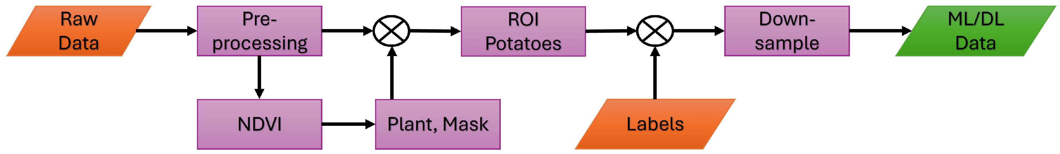
The raw data from the hyperspectral camera need to be calibrated and cleaned to remove the atmospheric effects and make the data independent of certain camera and light combinations. First, the radiance calibration is done using Equation 1, followed by Equation 2 for the reflectance calibration. A Savitzky-Golay smoothing filter is then applied using Equation 3. Some wavelength data are very noisy and are removed to clean the dataset for training the ML/DL algorithms. We then normalize the dataset. NDVI is calculated for each of the images using Equation 4, which is then used to create the potato mask using a certain threshold. We use this mask to get only the potato foliages which is downsampled using Equation 5 along with the ground-truth labels of the dataset. Our data was collected at a very low AGL and a small field, thus we downsample to recreate flying at a higher AGL which is more realistic for larger fields. The data is now prepared for Ml/DL analyses and we experiment with the algorithms mentioned in Section 2.3. Figure 9 shows the overall workflow of the steps performed to prepare the dataset for analysis. The preprocessing steps mentioned here, refers back to Figure 4.

Figure 9. Workflow diagram showing the steps involved in preparing the data for the ML/DL analyses. For the preprocessing steps, refer to Figure 4.

Figure 9. Workflow diagram showing the steps involved in preparing the data for the ML/DL analyses. For the preprocessing steps, refer to Figure 4.

3. Results

3.1. Dataset

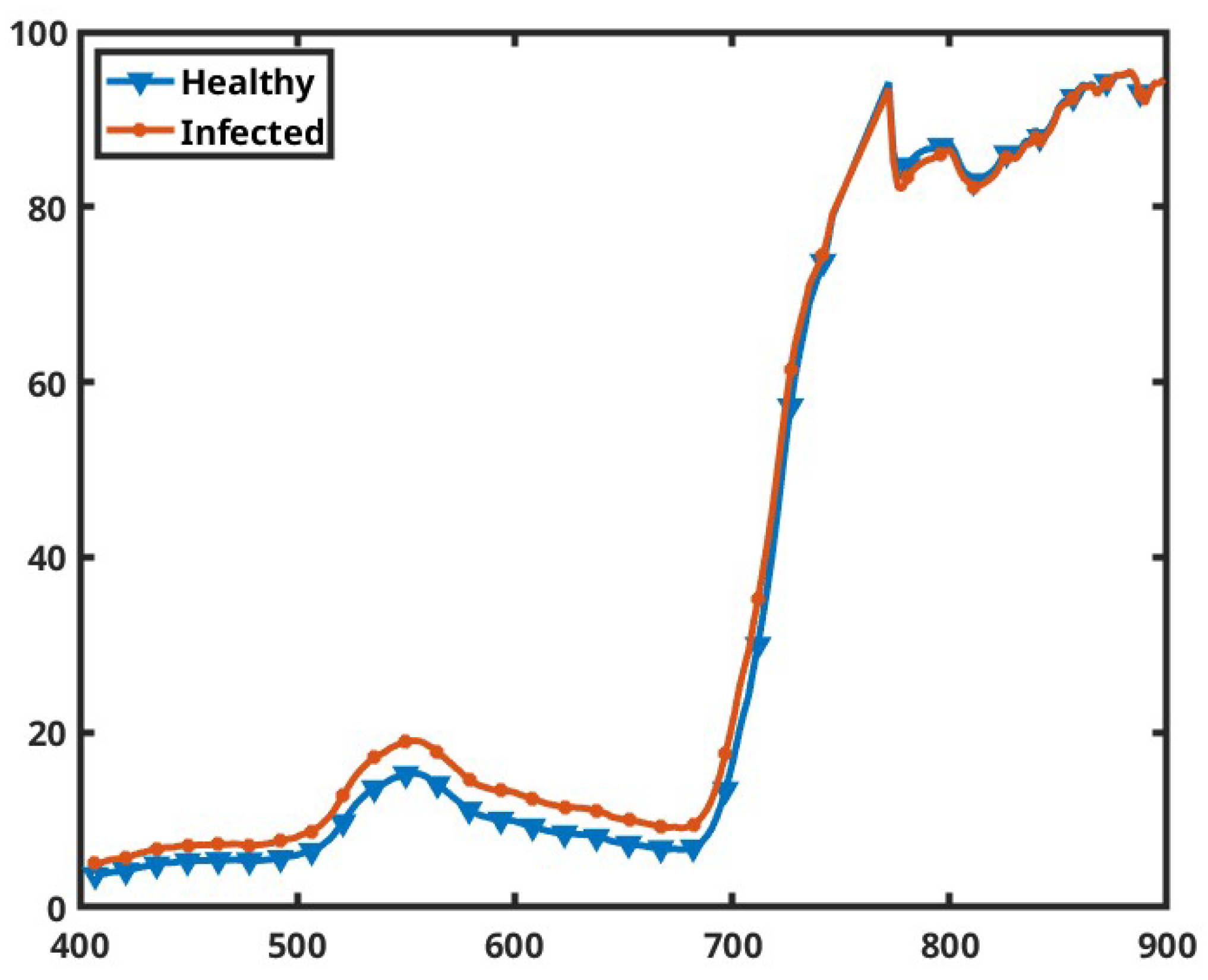
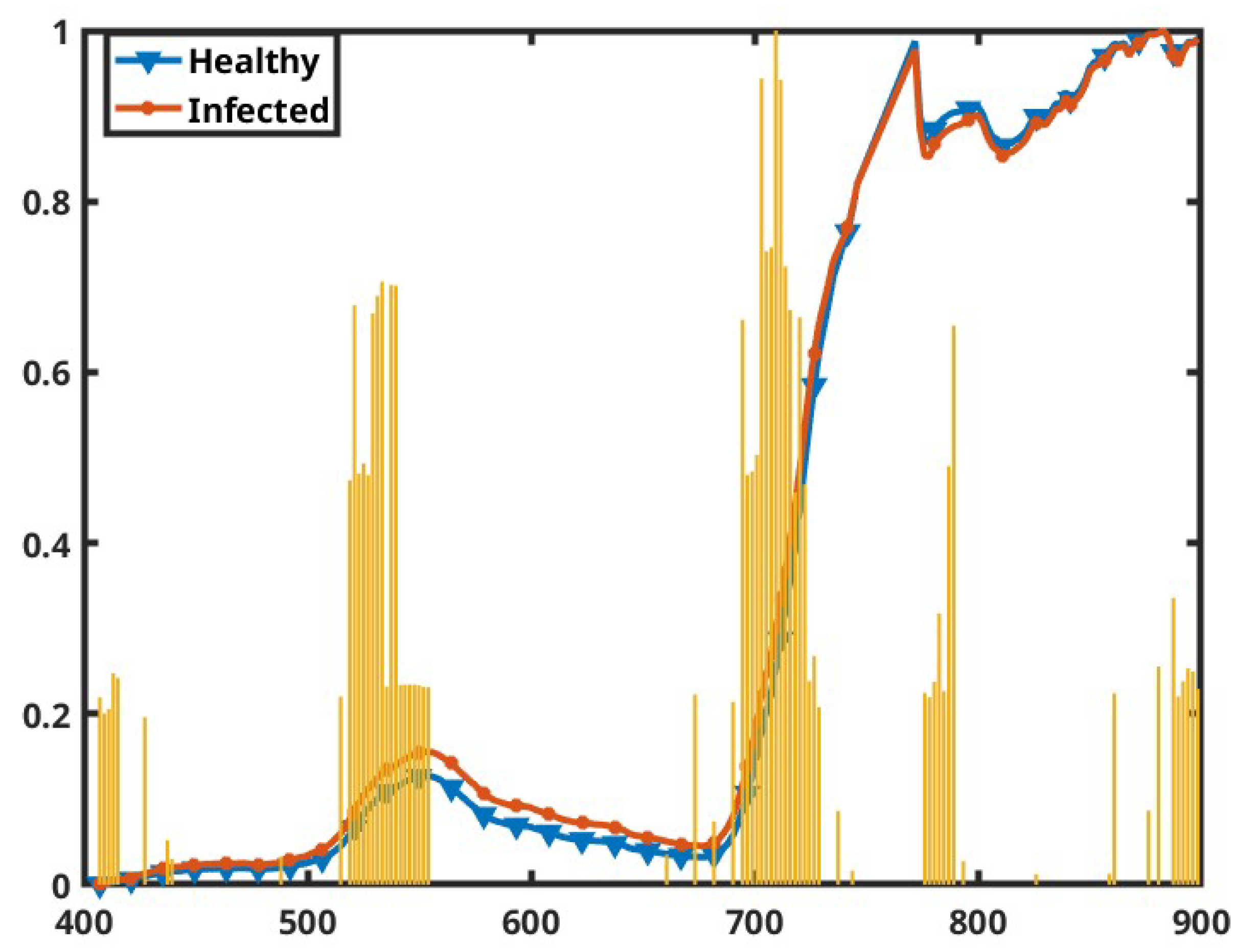
As mentioned in Section 2.1.3, we have 19 usable hyperspectral images and used 15 of them for model training and four for model testing. Some of the images did not contain any infected plants, thus four images were handpicked for testing the models. We are doing pixel-level detection, and after doing the pre-processing, cleaning, and downsampling, we ended up with 23844 hyperspectral pixels in total for all the images. 1794 of those pixels were labeled as infected and 177 of the infected pixels belong to the three test images. The other test image did not contain any infected pixels to test the confidence of the models. That leaves us with 1617 infected pixels for training and validation. To create a balanced dataset for training, we randomly picked 1617 healthy pixels from the pool of healthy pixels of the training images. Figure 10 shows the mean of all the healthy and infected pixels in the dataset. We notice some spectra differences in the visible region, however, the NIR region seems to be quite identical. It could be due to less water content differences in the plants. Note that the spectra are normalized in this figure.

Figure 10. The average spectra for all the healthy and infected pixels of the prepared dataset. The x-axis represents the wavelengths in nanometers and the y-axis shows the percentage of reflectance.

Figure 10. The average spectra for all the healthy and infected pixels of the prepared dataset. The x-axis represents the wavelengths in nanometers and the y-axis shows the percentage of reflectance.

3.2. Model Architectures and Optimizations

Bayes optimization [76] was employed with a maximum of 30 objective evaluations to fine-tune the hyperparameters of various models. For the SVM the optimal hyperparameters identified were a box constraint of 990.0862, a kernel scale of 77.3049, and a Gaussian kernel function. For the decision tree model, the optimal hyperparameters included a minimum leaf size of 27, a max number of splits value of 3151, and a split criterion of "deviance." In the KNN model, the optimal parameters were 13 for the number of neighbors and "correlation" as the distance metric. Logistic regression yielded optimal values with a lambda of 0.0104 and an "L2" regularization term.

A feedforward neural network (FNN) was developed with an input layer matching the number of features in the dataset (223). The architecture included two hidden layers containing 128 and 64 units, each followed by a ReLU activation function, and an output layer with a softmax activation function for classification.

A one-dimensional convolutional neural network (1D-CNN) was constructed. The architecture began with a convolutional layer utilizing a kernel size of 3, followed by batch normalization and a ReLU activation function. A max-pooling layer with a stride of 2 was applied to reduce dimensionality while preserving critical patterns. This was followed by a fully connected layer with 64 units and another ReLU activation layer. Finally, a fully connected layer with units equal to the number of classes (2) was added, followed by a softmax layer for predictions.

Both the FNN and CNN models were trained using the Adam optimizer for 50 epochs with a mini-batch size of 32. A 5-fold cross-validation strategy was implemented for all models where applicable to ensure robust performance evaluation.

3.3. Model Performances

We have evaluated all the optimized and trained models’ ability to identify the presence of potato virus Y in the plants using metrics such as accuracy, precision, recall, and F1-score, as shown in Table 2. Among all the models, the Convolutional Neural Network (CNN) achieved the highest scores in accuracy (0.962), precision (0.980), and F1-score (0.980). While the recall of CNN (0.980) is slightly lower than the highest observed value, it is the most reliable classifier for the task as the model is able to maintain high precision and recall. The overall balance across all metrics solidifies its position as the best model.

The Support Vector Machine (SVM) and Logistic Regression (LR) models also performed competitively, with accuracies of 0.956 and 0.952, respectively. Both models demonstrated high recall (0.987 and 0.988, respectively) and precision, resulting in F1 scores that were close to the top. These models are strong contenders and exhibit consistent performance. The highest observed recall value is 0.988 obtained by LR and Feedforward Neural Network (FNN).

In contrast, the Decision Tree (DT) and FNN models, while achieving high recall (both at 0.985 and 0.988, respectively), struggled with precision, resulting in lower F1 scores. This indicates that these models tend to produce more false positives compared to other methods. The K-Nearest Neighbors (KNN) model offered slightly better overall performance than DT and FNN, with a balanced F1 score of 0.926.

In summary, deep learning methods, particularly CNN outperformed the traditional approaches such as SVM, LR, and so on. Models like DT and FNN demonstrated notable strengths in recall but exhibited lower precision, which limits their overall effectiveness. However, in scenarios where the primary goal is to identify infected plants, these models can be advantageous. A higher recall ensures that most infected plants are correctly identified, even at the cost of mistakenly classifying some healthy plants as infected. These findings emphasize the critical importance of model selection based on specific objectives of the task and performance trade-offs.

Table 2. Classification results of Support Vector Machine (SVM), Decision Tree (DT), K-Nearest Neighbors (KNN), Logistic Regression (LR), Feedforward Neural Network (FNN), and Convolutional Neural Network (CNN) on the test set. The best result for each of the metrics is shown in bold.

Model	Accuracy	Precision	Recall	F1 score
SVM	0.956	0.966	0.987	0.977
DT	0.845	0.851	0.985	0.913
KNN	0.868	0.873	0.987	0.926
LR	0.952	0.962	0.988	0.975
FNN	0.804	0.804	0.988	0.887
CNN	0.962	0.980	0.980	0.980

Table 2. Classification results of Support Vector Machine (SVM), Decision Tree (DT), K-Nearest Neighbors (KNN), Logistic Regression (LR), Feedforward Neural Network (FNN), and Convolutional Neural Network (CNN) on the test set. The best result for each of the metrics is shown in bold.

Model	Accuracy	Precision	Recall	F1 score
SVM	0.956	0.966	0.987	0.977
DT	0.845	0.851	0.985	0.913
KNN	0.868	0.873	0.987	0.926
LR	0.952	0.962	0.988	0.975
FNN	0.804	0.804	0.988	0.887
CNN	0.962	0.980	0.980	0.980

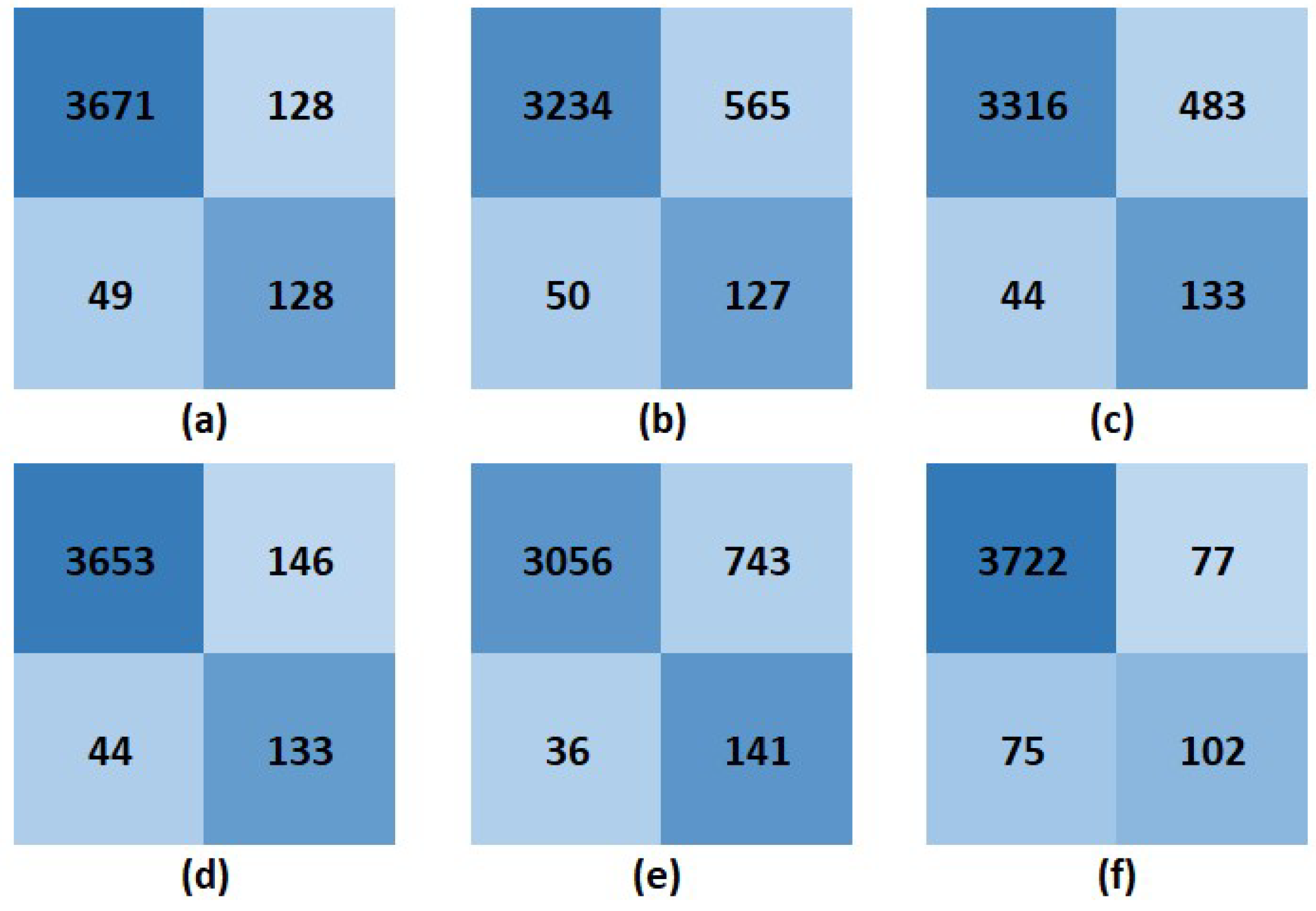
The confusion matrices summarizing the performance of the SVM, DT, KNN, LR, FNN, and CNN models are shown in Figure 11. The task for the models was to classify the healthy and infected hyperspectral pixels of the potato plants. Models like SVM, LR, and CNN demonstrate a strong balance between correctly identifying healthy plants (high specificity) and infected plants (moderate sensitivity), with CNN achieving the lowest false positive rate. FNN excels in sensitivity, with the fewest false negatives for infected plants, but struggles with specificity due to a high false-positive rate. In contrast, Decision Tree (DT) and KNN models show moderate performance, with higher false positives compared to SVM, LR, and CNN. Overall, SVM and LR provide the best trade-off between sensitivity and specificity, while CNN stands out for its reliability in identifying healthy plants, and FNN is most effective in detecting infected plants.

Figure 11. Confusion matrices for (a) Support Vector Machine, (b) Decision Tree, (c) K-Nearest Neighbors, (d) Logistic Regression, (e) Feedforward Neural Network, and (f) Convolutional Neural Network. These confusion matrices are reported by the respective models on the unseen test set.

Figure 11. Confusion matrices for (a) Support Vector Machine, (b) Decision Tree, (c) K-Nearest Neighbors, (d) Logistic Regression, (e) Feedforward Neural Network, and (f) Convolutional Neural Network. These confusion matrices are reported by the respective models on the unseen test set.

3.4. Prediction Analysis

The four images in the test set are images 26, 31, 39, and 43 from the dataset. The models were trained and tested only on the susceptible potatoes, thus in our prediction analysis we have used only the susceptible potatoes from the images. Note, we have used several PVY resistant varieties to reduce the spread of the PVY virus in the field. The predictions of the ML-DL models are shown for test image 39 in Figure 12 and for test image 43 in Figure 13. All the prediction stats are provided in Table 3.

Figure 12. Exploration of model performances on Image 39 of the test set. (a) RGB representation of the image after carefully curating the susceptible potatoes. (b) True labels of the PVY status for the image. Blue is healthy, green is infected, and yellow is background. There are 66 known infected pixels in the image shown in green color. The following subplots are the predictions of the image 31 using models: (c) Support Vector Machine, (d) Decision Tree, (e) K-Nearest Neighbors, (f) Logistic Regression, (g) Feedforward Neural Network, and (h) Convolutional Neural Network.

Figure 12. Exploration of model performances on Image 39 of the test set. (a) RGB representation of the image after carefully curating the susceptible potatoes. (b) True labels of the PVY status for the image. Blue is healthy, green is infected, and yellow is background. There are 66 known infected pixels in the image shown in green color. The following subplots are the predictions of the image 31 using models: (c) Support Vector Machine, (d) Decision Tree, (e) K-Nearest Neighbors, (f) Logistic Regression, (g) Feedforward Neural Network, and (h) Convolutional Neural Network.

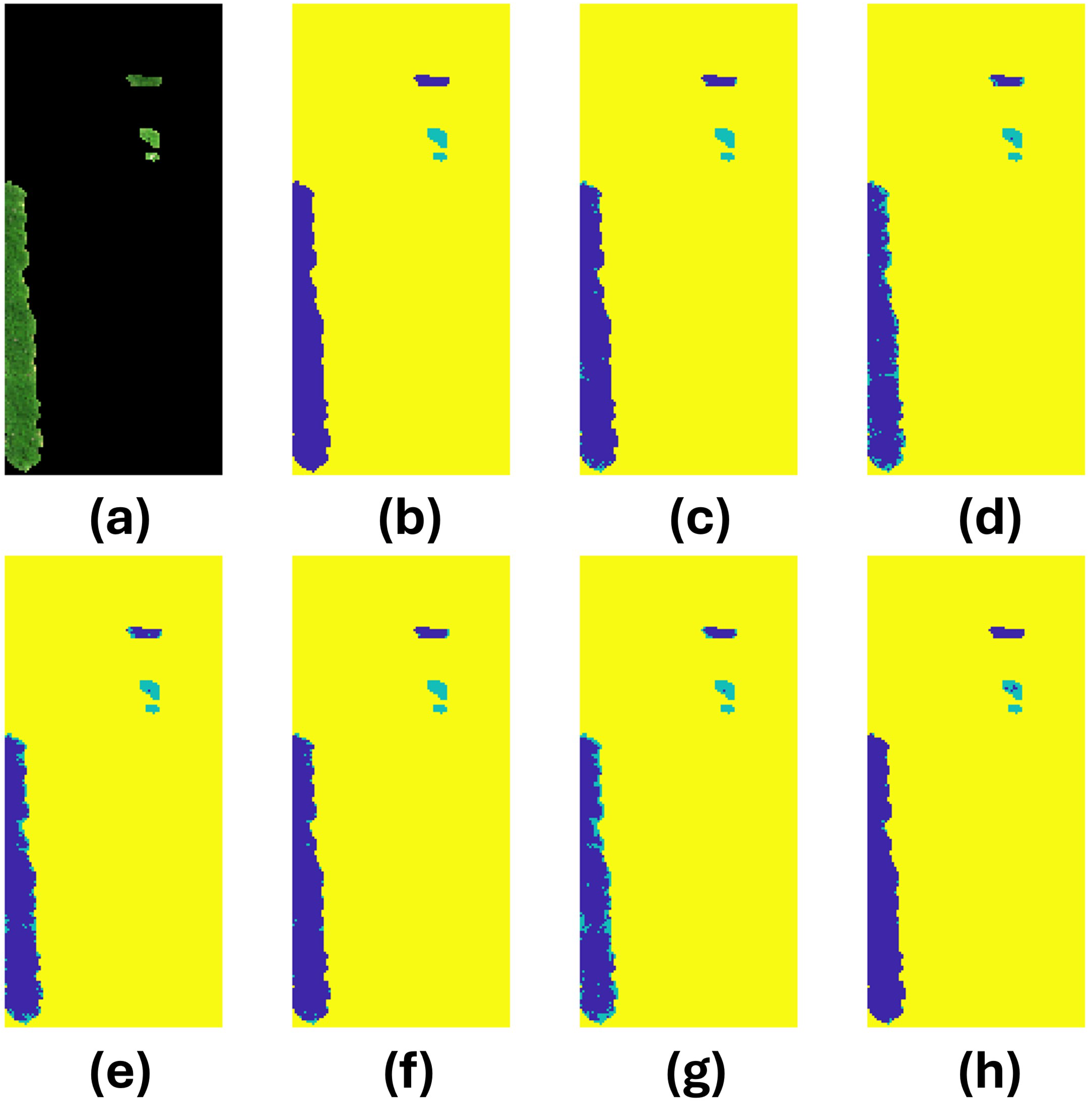
From Figure 12(b) we can see the infections are on the lower edges of the right plot. The blank portions on this plot are non-isolated plants and due to GPS issues their PVY status is unknown. Nonetheless, the plot is susceptible to PVY. From the predictions shown in subplots (c) – (h), we observe very satisfactory performance from all the models. Upon closer examination, it becomes evident that the FNN is over-predicting, identifying 303 pixels as infected. However, only 66 pixels were genuinely infected, with the FNN correctly classifying 65 of them. CNN on the other hand predicted 74 infected pixels, and correctly classified 61 infected pixels. Similarly, from Figure 13(b) we see there are no infections in this image. Other than the plot that can be seen here, the rest are resistant to PVY and thus omitted. Similar to the performance on the previous image, FNN predicted the highest number of infected pixels, however, this is not correct. CNN predicted the least number of infected pixels in the image. Since the predictions are sporadic, it is expected that we would achieve better results if we apply a low-pass filter to the predictions.

Figure 13. Exploration of model performances on Image 43 of the test set. (a) RGB representation of the image after carefully curating the susceptible potatoes. (b) True labels of the PVY status for the image. Blue is healthy, green is infected, and yellow is background. There are no known infected pixels in the image, as shown in the true labels. The following subplots are the predictions of the image 43 using models: (c) Support Vector Machine, (d) Decision Tree, (e) K-Nearest Neighbors, (f) Logistic Regression, (g) Feedforward Neural Network, and (h) Convolutional Neural Network.

Figure 13. Exploration of model performances on Image 43 of the test set. (a) RGB representation of the image after carefully curating the susceptible potatoes. (b) True labels of the PVY status for the image. Blue is healthy, green is infected, and yellow is background. There are no known infected pixels in the image, as shown in the true labels. The following subplots are the predictions of the image 43 using models: (c) Support Vector Machine, (d) Decision Tree, (e) K-Nearest Neighbors, (f) Logistic Regression, (g) Feedforward Neural Network, and (h) Convolutional Neural Network.

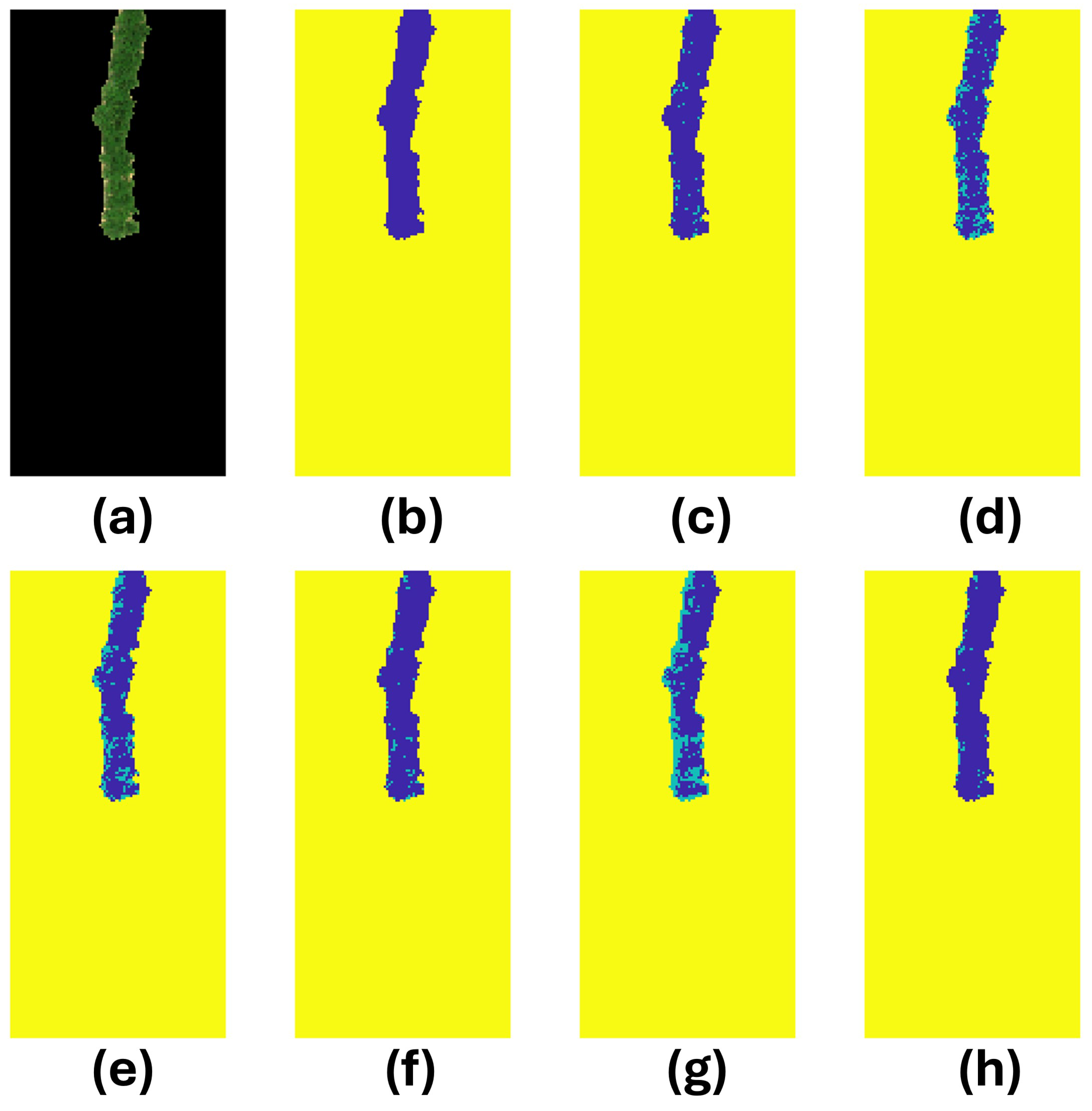
Table 3 takes a deep dive in the prediction stats of the test images. For Image 26, SVM achieved the highest accuracy ( 0.94%) with 36 correct predictions, however, LR achieveed the most correct predictions of 42. FNN significantly over-predicted with 38 correct predictions out of 77. CNN achieve high accuracy on image 31 while predicting 19 pixels correctly which is low compared to the other models. It is important to note that, CNN prohibits over-predicting, thus reducing false-positive predictions. DT and KNN also shows a pattern of over-prediction in images 39 and 43. To evaluate the robustness of the model performances, we introduced the test image 43 with no infections, and the all the models seem to struggle.

Table 3. Prediction analysis of different ML-DL models on the test sets. The table is showing the accuracy for each of the models on the images, along with the number of known infected pixels (# True Infected), the number of predicted infected pixels by the trained model (# Predicted Infected), and the number of correctly identified infected pixels (# Correct Infected).

Image	Model	Accuracy	# True Infected	# Predicted Infected	# Correct Infected
26	SVM	0.936232	54	40	36
	DT	0.817391		69	30
	KNN	0.886957		61	38
	LR	0.933333		53	42
	FNN	0.84058		77	38
	CNN	0.904348		23	22
31	SVM	0.935018	57	49	26
	DT	0.894103		95	32
	KNN	0.8929		92	30
	LR	0.927798		53	25
	FNN	0.880866		118	38
	CNN	0.942238		29	19
39	SVM	0.969717	66	111	66
	DT	0.876851		247	65
	KNN	0.902423		209	65
	LR	0.969717		111	66
	FNN	0.839166		303	65
	CNN	0.987887		74	61
43	SVM	0.957382	0	56	0
	DT	0.786149		281	0
	KNN	0.806697		254	0
	LR	0.952816		62	0
	FNN	0.70624		386	0
	CNN	0.959665		53	0

Table 3. Prediction analysis of different ML-DL models on the test sets. The table is showing the accuracy for each of the models on the images, along with the number of known infected pixels (# True Infected), the number of predicted infected pixels by the trained model (# Predicted Infected), and the number of correctly identified infected pixels (# Correct Infected).

Image	Model	Accuracy	# True Infected	# Predicted Infected	# Correct Infected
26	SVM	0.936232	54	40	36
	DT	0.817391		69	30
	KNN	0.886957		61	38
	LR	0.933333		53	42
	FNN	0.84058		77	38
	CNN	0.904348		23	22
31	SVM	0.935018	57	49	26
	DT	0.894103		95	32
	KNN	0.8929		92	30
	LR	0.927798		53	25
	FNN	0.880866		118	38
	CNN	0.942238		29	19
39	SVM	0.969717	66	111	66
	DT	0.876851		247	65
	KNN	0.902423		209	65
	LR	0.969717		111	66
	FNN	0.839166		303	65
	CNN	0.987887		74	61
43	SVM	0.957382	0	56	0
	DT	0.786149		281	0
	KNN	0.806697		254	0
	LR	0.952816		62	0
	FNN	0.70624		386	0
	CNN	0.959665		53	0

3.5. Feature Importance

Hyperspectral imaging has the potential to identify the PVY virus in potato fields. However, hyperspectral cameras provide densely sampled spectral data, which includes redundant or less significant bands. By pinpointing the most relevant bands, we can design cost-effective multispectral cameras tailored to the task of classifying the PVY virus. To identify the most relevant bands we have utilized six different feature ranking methods. They are: chi-square test [81] - evaluates the independence between each feature and target variable; minimum redundancy maximum relevance (MRMR) [82] - balances relevance and redundancy by selecting highly correlated features with the target variable but minimally correlated with each other; f-test [83] - evaluates the variance ratio between classes for each feature; rank features [84] - rank key features based on independent evaluation criteria; neighborhood component analysis (NCA) [85] - learns feature weights by optimizing a distance-based classification objective; and reliefF algorithm [85] - ranks features by considering their ability to differentiate between instances that are near each other. First, we rank the features using all these six methods independently, then normalize the score to a scale of 0 to 1. Finally, we calculated the cumulative importance of the features as shown in bar graphs in Figure 14.

The cumulative importance identifies five key regions across the spectrum centered at 411 nm, 533 nm, 709 nm, 782 nm, and 892 nm. The first two bands (411 nm and 533 nm) correspond to the spectral features influenced by the chlorophyll contents of the plants. The middle band (709 nm) identifies the critical red-edge spectra. The last two bands (782 nm and 892 nm) are the NIR bands responsible for the water content and cell structure of the plants. For reference, the mean-normalized spectra of the healthy and infected plants are also illustrated in the figure.

Figure 14. Most relevant bands across the spectra shown in the yellow bar-graphs. The line plots are the normalized mean spectra of the healthy and infected plants as indicated by the color legends - shown for reference. The x-axis represents the wavelengths in nanometers and the y-axis represents the normalized scale from 0 to 1.

Figure 14. Most relevant bands across the spectra shown in the yellow bar-graphs. The line plots are the normalized mean spectra of the healthy and infected plants as indicated by the color legends - shown for reference. The x-axis represents the wavelengths in nanometers and the y-axis represents the normalized scale from 0 to 1.

4. Discussion

The aim of this research is to develop an artificial intelligence based system that is capable of detecting PVY efficiently. It is well established that a huge amount of dataset is needed for generalizing any trained ML-DL models. A few varieties from one growing season have been used for this work. Though we have observed promising performance from the trained models, it is suspected that the performance might vary for a different variety and environmental conditions. We are working with different seed potato producers to help us collect more data. The next challenge is to label the data - it is very time-consuming and needs an expert to do a visual inspection and perform an ELISA test to identify the presence of the PVY virus. This is needed to create the ground truth to train the ML-DL models.

Unfortunately, we faced a magnetometer IMU issue with our camera, and by the time we realized the issue it was late in the season to do another flight and capture the data. This resulted in a GPS error and we were not able to perform geo-rectification on the hyperspectral images and create an orthomosaic map. An orthomosaic map is a large detailed georeferenced image of the target location created by carefully stitching the smaller images. Fortunately, after a few days, we flew another UAV with a multispectral camera that helped us manually stitch an orthomosaic map from the distorted HSI data.

We have trained our ML-DL models on a pixel-based classification task, however, it might be interesting to train the models on small-image patches that will cover more surface area, potentially providing a robust performance. Our current dataset is highly imbalanced, i.e. a few infected plants compared to healthy plants. Thus it would be helpful to have a dataset with more infected plants. It would be intriguing to investigate the changes in the model performances by the changes in the day of data collection from the growing season. There is also the scope of exploring the time-series algorithms, however might not be realistic, given that the producers would benefit from ar early-season prediction, rather than at the end of the season. Frequent HSI data over the growing season would benefit the research providing profound knowledge on how soon the PVY can be detected. The rate of the PVY spread across the field can also be estimated from frequent data collection.

Refer back to Figure 11 for the confusion matrices for all the experimental models on the test set. This level of accuracy is only detecting 80% of the diseased plants in the worst case, and has a only a 50% confidence rate when we detect a diseased plant. Because they are working to keep the disease rate in fields to less than 0.5% at this time it is not sufficient accuracy for management of the disease in seed potato or production fields as the primary tool. We have an issue of predictive power. Currently if we say something is positive we are only 50% confident in that prediction at best. It is a start, and also it may be accurate enough for field certification using a UAV system.

All the models trained on this work are based on supervised learning, i.e. the model is trained with an input having the respective output. However, it is quite expensive to create such a dataset, thus we would be interested in exploring semi-supervised and unsupervised learning models. A semi-supervised learning technique is training a model where some of the inputs are labeled and most of them are unlabeled, An unsupervised learning method involves model training with unlabeled inputs. Though we observed a high precision and recall in our hyperparameter-optimized trained models, it would be compelling to explore complex deep NNs. Different dimensionality reduction techniques need to be employed to address the ’big data’ volume of large HSI data.

5. Conclusions

Early detection of PVY in seed potatoes is crucial to minimize economic yield losses and ensure food security around the globe. In this paper, we present machine learning insights into HSI data utilizing UAVs for detecting PVY. We collected and published a new hyperspectral PVY dataset containing the ground truth labels for healthy and infected plants. The HSI data has 300 spectral bands and ranges from 400-1000 nm, however, we have curated the spectral bands to address the noise and absorptions and had 223 spectral bands. While the data is highly imbalanced, we have used a subset of the data to create a balanced dataset for training the supervised ML-DL models. We have trained several ML-DL algorithms and obtained an accuracy of 0.962% with the CNN model. The CNN model performed the best in predicting the healthy plants with a precision of 0.98% and the FNN model is better at predicting the infected plants with a recall of 0.988%. The overall F1-score of the CNN model is 0.98%, making it a robust trained model for the classification of PVY. We have also investigated all the spectra and discovered that only a few of those spectra contain the most relevant information in classifying the PVY. While there is room for improvement and generalizing the models with a bigger dataset, the results are promising and show the potential of building a customized multispectral camera integrated with a UAV focusing on early prediction of PVY.

References

- Crosslin, J.M. PVY: An old enemy and a continuing challenge. American journal of potato research 2013, 90, 2–6. [Google Scholar] [CrossRef]
- Glais, L.; Bellstedt, D.U.; Lacomme, C. Diversity, characterisation and classification of PVY. Potato virus Y: biodiversity, pathogenicity, epidemiology and management, 2017; pp. 43–76. [Google Scholar]
- Wani, S.; Saleem, S.; Nabi, S.U.; Ali, G.; Paddar, B.A.; Hamid, A. Distribution and molecular characterization of potato virus Y (PVY) strains infecting potato (Solanum tuberosum) crop in Kashmir (India). VirusDisease 2021, 32, 784–788. [Google Scholar] [CrossRef] [PubMed]
- Dupuis, B.; Nkuriyingoma, P.; Ballmer, T. Economic impact of potato virus Y (PVY) in Europe. Potato Research 2024, 67, 55–72. [Google Scholar] [CrossRef]
- Glais, L.; Chikh Ali, M.; Karasev, A.V.; Kutnjak, D.; Lacomme, C. Detection and diagnosis of PVY. Potato virus Y: Biodiversity, pathogenicity, epidemiology and management, 2017; pp. 103–139. [Google Scholar]
- MacKenzie, T.D.; Nie, X.; Singh, M. RT-PCR and real-time RT-PCR methods for the detection of potato virus Y in potato leaves and tubers. Plant Virology Protocols: New Approaches to Detect Viruses and Host Responses, 2015; pp. 13–26. [Google Scholar]
- Kumar, R.; Tiwari, R.K.; Sundaresha, S.; Kaundal, P.; Raigond, B. Potato viruses and their management. In Sustainable management of potato pests and diseases; Springer, 2022; pp. 309–335.
- Afzaal, H.; Farooque, A.A.; Schumann, A.W.; Hussain, N.; McKenzie-Gopsill, A.; Esau, T.; Abbas, F.; Acharya, B. Detection of a potato disease (early blight) using artificial intelligence. Remote Sensing 2021, 13, 411. [Google Scholar] [CrossRef]
- Sun, C.; Zhou, J.; Ma, Y.; Xu, Y.; Pan, B.; Zhang, Z. A review of remote sensing for potato traits characterization in precision agriculture. Frontiers in Plant Science 2022, 13, 871859. [Google Scholar] [CrossRef]
- Moslemkhani, C.; Hassani, F.; Azar, E.N.; Khelgatibana, F. Potential of spectroscopy for differentiation between PVY infected and healthy potato plants. Crop Prot 2019, 8, 143–151. [Google Scholar]
- Castro, R.C. Prediction of yield and diseases in crops using vegetation indices through satellite image processing. In Proceedings of the 2024 IEEE Technology and Engineering Management Society (TEMSCON LATAM). IEEE; 2024; pp. 1–6. [Google Scholar]
- Mukiibi, A.; Machakaire, A.; Franke, A.; Steyn, J. A Systematic Review of Vegetation Indices for Potato Growth Monitoring and Tuber Yield Prediction from Remote Sensing. Potato Research, 2024; pp. 1–40. [Google Scholar]
- Khojastehnazhand, M.; Khoshtaghaza, M.H.; Mojaradi, B.; Rezaei, M.; Goodarzi, M.; Saeys, W. Comparison of visible–near infrared and short wave infrared hyperspectral imaging for the evaluation of rainbow trout freshness. Food Research International 2014, 56, 25–34. [Google Scholar] [CrossRef]
- Nesar, S.; Whitaker, B.; Zidack, N.; Nugent, P. Hyperspectral remote sensing approach for rapid detection of potato virus Y. In Proceedings of the Photonic Technologies in Plant and Agricultural Science. SPIE, Vol. 12879; 2024; pp. 79–83. [Google Scholar]
- Jiang, M.; Li, Y.; Song, J.; Wang, Z.; Zhang, L.; Song, L.; Bai, B.; Tu, K.; Lan, W.; Pan, L. Study on black spot disease detection and pathogenic process visualization on winter jujubes using hyperspectral imaging system. Foods 2023, 12, 435. [Google Scholar] [CrossRef]
- Zhang, X.; Vinatzer, B.A.; Li, S. Hyperspectral imaging analysis for early detection of tomato bacterial leaf spot disease. Scientific Reports 2024, 14, 27666. [Google Scholar] [CrossRef]
- Nguyen, C.; Sagan, V.; Maimaitiyiming, M.; Maimaitijiang, M.; Bhadra, S.; Kwasniewski, M.T. Early detection of plant viral disease using hyperspectral imaging and deep learning. Sensors 2021, 21, 742. [Google Scholar] [CrossRef]
- Yadav, P.K.; Burks, T.; Frederick, Q.; Qin, J.; Kim, M.; Ritenour, M.A. Citrus disease detection using convolution neural network generated features and Softmax classifier on hyperspectral image data. Frontiers in Plant Science 2022, 13, 1043712. [Google Scholar] [CrossRef] [PubMed]
- Li, Y.; Al-Sarayreh, M.; Irie, K.; Hackell, D.; Bourdot, G.; Reis, M.M.; Ghamkhar, K. Identification of weeds based on hyperspectral imaging and machine learning. Frontiers in Plant Science 2021, 11, 611622. [Google Scholar] [CrossRef] [PubMed]
- Bharadwaj, S.; Prabhu, A.; Solanki, V. Automating Weed Detection Through Hyper Spectral Image Analysis. In Proceedings of the 2024 International Conference on Optimization Computing and Wireless Communication (ICOCWC). IEEE; 2024; pp. 1–5. [Google Scholar]
- Wei, D.; Huang, Y.; Chunjiang, Z.; Xiu, W. Identification of seedling cabbages and weeds using hyperspectral imaging. International Journal of Agricultural and Biological Engineering 2015, 8, 65–72. [Google Scholar]
- Zuo, J.; Peng, Y.; Li, Y.; Chen, Y.; Yin, T. Advancements in Hyperspectral Imaging for Assessing Nutritional Parameters in Muscle Food: Current Research and Future Trends. Journal of Agricultural and Food Chemistry 2024. [Google Scholar] [CrossRef]
- Peng, Y.; Wang, L.; Zhao, L.; Liu, Z.; Lin, C.; Hu, Y.; Liu, L. Estimation of soil nutrient content using hyperspectral data. Agriculture 2021, 11, 1129. [Google Scholar] [CrossRef]
- Teo, V.X.; Dhandapani, S.; Ang Jie, R.; Philip, V.S.; Teo Ju Teng, M.; Zhang, S.; Park, B.S.; Olivo, M.; Dinish, U. Early detection of N, P, K deficiency in Choy Sum using hyperspectral imaging-based spatial spectral feature mining. Frontiers in Photonics 2024, 5, 1418246. [Google Scholar] [CrossRef]
- Eshkabilov, S.; Stenger, J.; Knutson, E.N.; Küçüktopcu, E.; Simsek, H.; Lee, C.W. Hyperspectral image data and waveband indexing methods to estimate nutrient concentration on lettuce (Lactuca sativa L.) cultivars. Sensors 2022, 22, 8158. [Google Scholar] [CrossRef]
- Wang, Y.; Zhang, Y.; Yuan, Y.; Zhao, Y.; Nie, J.; Nan, T.; Huang, L.; Yang, J. Nutrient content prediction and geographical origin identification of red raspberry fruits by combining hyperspectral imaging with chemometrics. Frontiers in Nutrition 2022, 9, 980095. [Google Scholar] [CrossRef]
- Caporaso, N.; Whitworth, M.B.; Fisk, I.D. Protein content prediction in single wheat kernels using hyperspectral imaging. Food chemistry 2018, 240, 32–42. [Google Scholar] [CrossRef]
- Qiao, M.; He, X.; Cheng, X.; Li, P.; Luo, H.; Tian, Z.; Guo, H. Exploiting hierarchical features for crop yield prediction based on 3-d convolutional neural networks and multikernel gaussian process. IEEE Journal of Selected Topics in Applied Earth Observations and Remote Sensing 2021, 14, 4476–4489. [Google Scholar] [CrossRef]
- Zhang, Z.; Qu, Y.; Ma, F.; Lv, Q.; Zhu, X.; Guo, G.; Li, M.; Yang, W.; Que, B.; Zhang, Y.; et al. Integrating high-throughput phenotyping and genome-wide association studies for enhanced drought resistance and yield prediction in wheat. New Phytologist 2024, 243, 1758–1775. [Google Scholar] [CrossRef] [PubMed]
- Gutiérrez, S.; Wendel, A.; Underwood, J. Ground based hyperspectral imaging for extensive mango yield estimation. Computers and Electronics in Agriculture 2019, 157, 126–135. [Google Scholar] [CrossRef]
- Zhou, Y.; Biswas, A.; Hong, Y.; Chen, S.; Hu, B.; Shi, Z.; Guo, Y.; Li, S. Enhancing soil profile analysis with soil spectral libraries and laboratory hyperspectral imaging. Geoderma 2024, 450, 117036. [Google Scholar] [CrossRef]
- Xu, S.; Wang, M.; Shi, X. Hyperspectral imaging for high-resolution mapping of soil carbon fractions in intact paddy soil profiles with multivariate techniques and variable selection. Geoderma 2020, 370, 114358. [Google Scholar] [CrossRef]
- Zhao, S.; Qiu, Z.; He, Y. Transfer learning strategy for plastic pollution detection in soil: Calibration transfer from high-throughput HSI system to NIR sensor. Chemosphere 2021, 272, 129908. [Google Scholar] [CrossRef]
- Jia, S.; Li, H.; Wang, Y.; Tong, R.; Li, Q. Hyperspectral imaging analysis for the classification of soil types and the determination of soil total nitrogen. Sensors 2017, 17, 2252. [Google Scholar] [CrossRef]
- Griffel, L.M.; Delparte, D.; Whitworth, J.; Bodily, P.; Hartley, D. Evaluation of artificial neural network performance for classification of potato plants infected with potato virus Y using spectral data on multiple varieties and genotypes. Smart Agricultural Technology 2023, 3, 100101. [Google Scholar] [CrossRef]
- Polder, G.; Blok, P.M.; De Villiers, H.A.; Van der Wolf, J.M.; Kamp, J. Potato virus Y detection in seed potatoes using deep learning on hyperspectral images. Frontiers in plant science 2019, 10, 209. [Google Scholar] [CrossRef]
- Wang, Y.; Duan, H. Classification of hyperspectral images by SVM using a composite kernel by employing spectral, spatial and hierarchical structure information. Remote Sensing 2018, 10, 441. [Google Scholar] [CrossRef]
- Hasan, H.; Shafri, H.Z.; Habshi, M. A comparison between support vector machine (SVM) and convolutional neural network (CNN) models for hyperspectral image classification. In Proceedings of the IOP Conference Series: Earth and Environmental Science. IOP Publishing, Vol. 357; 2019; p. 012035. [Google Scholar]
- Wang, K.; Cheng, L.; Yong, B. Spectral-similarity-based kernel of SVM for hyperspectral image classification. Remote Sensing 2020, 12, 2154. [Google Scholar] [CrossRef]
- Guo, Y.; Yin, X.; Zhao, X.; Yang, D.; Bai, Y. Hyperspectral image classification with SVM and guided filter. EURASIP Journal on Wireless Communications and Networking 2019, 2019, 1–9. [Google Scholar] [CrossRef]
- Wang, A.; Wang, Y.; Chen, Y. Hyperspectral image classification based on convolutional neural network and random forest. Remote sensing letters 2019, 10, 1086–1094. [Google Scholar] [CrossRef]
- Wang, L.; Wang, Q. Fast spatial-spectral random forests for thick cloud removal of hyperspectral images. International Journal of Applied Earth Observation and Geoinformation 2022, 112, 102916. [Google Scholar] [CrossRef]
- Tong, F.; Zhang, Y. Exploiting spectral–spatial information using deep random forest for hyperspectral imagery classification. IEEE Geoscience and Remote Sensing Letters 2021, 19, 1–5. [Google Scholar] [CrossRef]
- Zhang, Y.; Cao, G.; Li, X.; Wang, B.; Fu, P. Active semi-supervised random forest for hyperspectral image classification. Remote Sensing 2019, 11, 2974. [Google Scholar] [CrossRef]
- Chang, Y.; Yan, L.; Fang, H.; Zhong, S.; Liao, W. HSI-DeNet: Hyperspectral image restoration via convolutional neural network. IEEE Transactions on Geoscience and Remote Sensing 2018, 57, 667–682. [Google Scholar] [CrossRef]
- He, M.; Li, B.; Chen, H. Multi-scale 3D deep convolutional neural network for hyperspectral image classification. In Proceedings of the 2017 IEEE International Conference on Image Processing (ICIP). IEEE; 2017; pp. 3904–3908. [Google Scholar]
- Zhu, J.; Fang, L.; Ghamisi, P. Deformable convolutional neural networks for hyperspectral image classification. IEEE Geoscience and Remote Sensing Letters 2018, 15, 1254–1258. [Google Scholar] [CrossRef]
- Ayesha, S.; Hanif, M.K.; Talib, R. Overview and comparative study of dimensionality reduction techniques for high dimensional data. Information Fusion 2020, 59, 44–58. [Google Scholar] [CrossRef]
- Mayer, M. Early detection of virus infections in potato by aphids and infrared remote sensing. SLU, Dept. of Crop Production Ecology, 2017. [Google Scholar]
- Griffel, L.; Delparte, D.; Edwards, J. Using Support Vector Machines classification to differentiate spectral signatures of potato plants infected with Potato Virus Y. Computers and electronics in agriculture 2018, 153, 318–324. [Google Scholar] [CrossRef]
- Chen, H.; Han, Y.; Liu, Y.; Liu, D.; Jiang, L.; Huang, K.; Wang, H.; Guo, L.; Wang, X.; Wang, J.; et al. Classification models for Tobacco Mosaic Virus and Potato Virus Y using hyperspectral and machine learning techniques. Frontiers in Plant Science 2023, 14, 1211617. [Google Scholar] [CrossRef]
- AgEagle Aerial Systems. Altum-PT Camera. https://ageagle.com/drone-sensors/altum-pt-camera/. Accessed: 2024-12-20.
- Funke, C.N.; Tran, L.T.; Karasev, A.V. Screening Three Potato Cultivars for Resistance to Potato Virus Y Strains: Broad and Strain-Specific Sources of Resistance. American Journal of Potato Research 2024, 101, 132–141. [Google Scholar] [CrossRef]
- Kondakova, O.; Butenko, K.; Skurat, E.; Drygin, Y.F. Molecular diagnostics of potato infections with PVY and PLRV by immunochromatography. Moscow University Biological Sciences Bulletin 2016, 71, 39–44. [Google Scholar] [CrossRef]
- Singh, R.; Santos-Rojas, J. Detection of potato virus Y in primarily infected mature plants by ELISA, indicator host, and visual indexing. Canadian plant disease survey 1983, 63, 39–44. [Google Scholar]
- Vision Aerial. Vector Hexacopter Drone. https://visionaerial.com/vector/. Accessed: 2024-12-18.
- Resonon. Pika L Hyperspectral Imaging Camera. https://resonon.com/Pika-L. Accessed: 2024-12-18.
- Resonon. Hyperspectral Imaging Software. https://resonon.com/software. Accessed: 2024-12-18.
- DJI. Matrice 600 - Product Support. https://www.dji.com/support/product/matrice600. Accessed: 2024-12-20.
- Liang, S. Quantitative remote sensing of land surfaces; John Wiley & Sons, 2005.
- Schowengerdt, R.A. Remote sensing: models and methods for image processing; elsevier, 2006.
- Savitzky, A.; Golay, M.J. Smoothing and differentiation of data by simplified least squares procedures. Analytical chemistry 1964, 36, 1627–1639. [Google Scholar] [CrossRef]
- Huang, S.; Tang, L.; Hupy, J.P.; Wang, Y.; Shao, G. A commentary review on the use of normalized difference vegetation index (NDVI) in the era of popular remote sensing. Journal of Forestry Research 2021, 32, 1–6. [Google Scholar] [CrossRef]
- Fageria, M.S.; Singh, M.; Nanayakkara, U.; Pelletier, Y.; Nie, X.; Wattie, D. Monitoring current-season spread of Potato virus Y in potato fields using ELISA and real-time RT-PCR. Plant Disease 2013, 97, 641–644. [Google Scholar] [CrossRef]
- Singh, R.; Somerville, T. Evaluation of the enzyme-amplified ELISA for the detection of potato viruses A, M, S, X, Y, and leafroll. American Potato Journal 1992, 69, 21–30. [Google Scholar] [CrossRef]
- CVAT.ai. CVAT: Computer Vision Annotation Tool. https://www.cvat.ai/. Accessed: 2024-12-20.
- Hearst, M.A.; Dumais, S.T.; Osuna, E.; Platt, J.; Scholkopf, B. Support vector machines. IEEE Intelligent Systems and their applications 1998, 13, 18–28. [Google Scholar] [CrossRef]
- Myles, A.J.; Feudale, R.N.; Liu, Y.; Woody, N.A.; Brown, S.D. An introduction to decision tree modeling. Journal of Chemometrics: A Journal of the Chemometrics Society 2004, 18, 275–285. [Google Scholar] [CrossRef]
- Batista, G.; Silva, D.F.; et al. How k-nearest neighbor parameters affect its performance. In Proceedings of the Argentine symposium on artificial intelligence. Citeseer; 2009; pp. 1–12. [Google Scholar]
- Kleinbaum, D.G.; Dietz, K.; Gail, M.; Klein, M.; Klein, M. Logistic regression; Springer, 2002.
- Goodfellow, I. Deep learning, 2016.
- Aloysius, N.; Geetha, M. A review on deep convolutional neural networks. In Proceedings of the 2017 international conference on communication and signal processing (ICCSP). IEEE; 2017; pp. 0588–0592. [Google Scholar]
- Liao, L.; Li, H.; Shang, W.; Ma, L. An empirical study of the impact of hyperparameter tuning and model optimization on the performance properties of deep neural networks. ACM Transactions on Software Engineering and Methodology (TOSEM) 2022, 31, 1–40. [Google Scholar] [CrossRef]
- Yang, L.; Shami, A. On hyperparameter optimization of machine learning algorithms: Theory and practice. Neurocomputing 2020, 415, 295–316. [Google Scholar] [CrossRef]
- Nesar, S.B.; Whitaker, B.M.; Maher, R.C. Machine Learning Analysis on Gunshot Recognition. In Proceedings of the 2024 Intermountain Engineering, Technology and Computing (IETC). IEEE; 2024; pp. 249–254. [Google Scholar]
- Bayes, T. An essay towards solving a problem in the doctrine of chances. Biometrika 1958, 45, 296–315. [Google Scholar] [CrossRef]
- Sokolova, M.; Lapalme, G. A systematic analysis of performance measures for classification tasks. Information processing & management 2009, 45, 427–437. [Google Scholar]
- Powers, D.M. Evaluation: from precision, recall and F-measure to ROC, informedness, markedness and correlation. arXiv preprint arXiv:2010.16061, arXiv:2010.16061 2020.
- Salimi, A.; Ziaii, M.; Amiri, A.; Zadeh, M.H.; Karimpouli, S.; Moradkhani, M. Using a Feature Subset Selection method and Support Vector Machine to address curse of dimensionality and redundancy in Hyperion hyperspectral data classification. The Egyptian Journal of Remote Sensing and Space Science 2018, 21, 27–36. [Google Scholar] [CrossRef]
- Jović, A.; Brkić, K.; Bogunović, N. A review of feature selection methods with applications. In Proceedings of the 2015 38th international convention on information and communication technology, electronics and microelectronics (MIPRO). Ieee; 2015; pp. 1200–1205. [Google Scholar]
- Liu, H.; Motoda, H. Computational methods of feature selection; CRC press, 2007.
- Peng, H.; Long, F.; Ding, C. Feature selection based on mutual information criteria of max-dependency, max-relevance, and min-redundancy. IEEE Transactions on pattern analysis and machine intelligence 2005, 27, 1226–1238. [Google Scholar] [CrossRef]
- Golugula, A.; Lee, G.; Madabhushi, A. Evaluating feature selection strategies for high dimensional, small sample size datasets. In Proceedings of the 2011 Annual International conference of the IEEE engineering in medicine and biology society. IEEE; 2011; pp. 949–952. [Google Scholar]
- Liu, H.; Motoda, H. Feature selection for knowledge discovery and data mining; Vol. 454, Springer science & business media, 2012.
- Tuncer, T.; Ertam, F. Neighborhood component analysis and reliefF based survival recognition methods for Hepatocellular carcinoma. Physica A: Statistical Mechanics and its Applications 2020, 540, 123143. [Google Scholar] [CrossRef]
Disclaimer/Publisher’s Note: The statements, opinions and data contained in all publications are solely those of the individual author(s) and contributor(s) and not of MDPI and/or the editor(s). MDPI and/or the editor(s) disclaim responsibility for any injury to people or property resulting from any ideas, methods, instructions or products referred to in the content. |
© 2024 by the authors. Licensee MDPI, Basel, Switzerland. This article is an open access article distributed under the terms and conditions of the Creative Commons Attribution (CC BY) license (https://creativecommons.org/licenses/by/4.0/).
Copyright: This open access article is published under a Creative Commons CC BY 4.0 license, which permit the free download, distribution, and reuse, provided that the author and preprint are cited in any reuse.