
Submitted:
04 May 2025
Posted:
06 May 2025
Read the latest preprint version here
Abstract
Entanglement swapping is one of the most peculiar quantum mechanical phenomena, which is a key technology to realize long-distance quantum communication and build quantum networks, and has extensive and important applications in quantum information processing. In this paper, we combine some principles of classical physics with those of quantum mechanics to propose a new theoretical framework and design a new algorithm for entanglement swapping based on it, the basic idea of which is to construct two entangled states after entanglement swapping from all possible observations. We demonstrate the algorithm by the entanglement swapping between two bipartite entangled states, and derive the results of entanglement swapping between two Bell states, which are consistent with those obtained through algebraic calculations. Our work not only provide new perspectives for exploring quantum mechanical phenomena and the principles behind them, but also can trigger in-depth exploration of the mysteries of nature.
Keywords:
1. Introduction
2. Entanglement Swapping Between Two Bell States
3. The New Algorithm for Entanglement Swapping
3.1. The Theoretical Framework

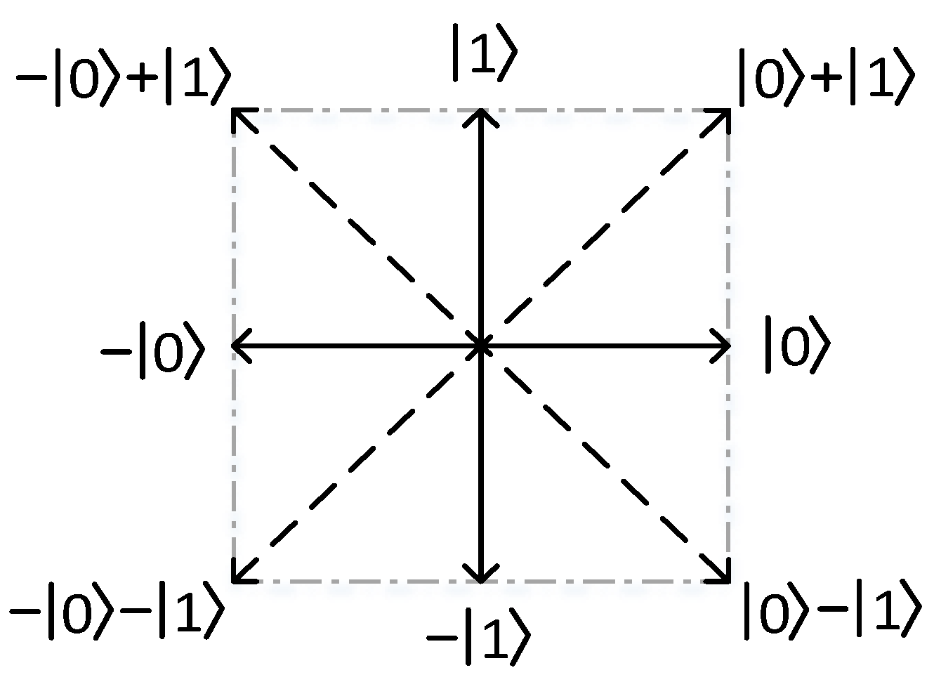
3.2. The Proposed Algorithm

| Joint state | Combinations of the states of two subsystems |
|---|---|
| 1 or | |
| 2 or | |
| 3 or | |
| 4 or |
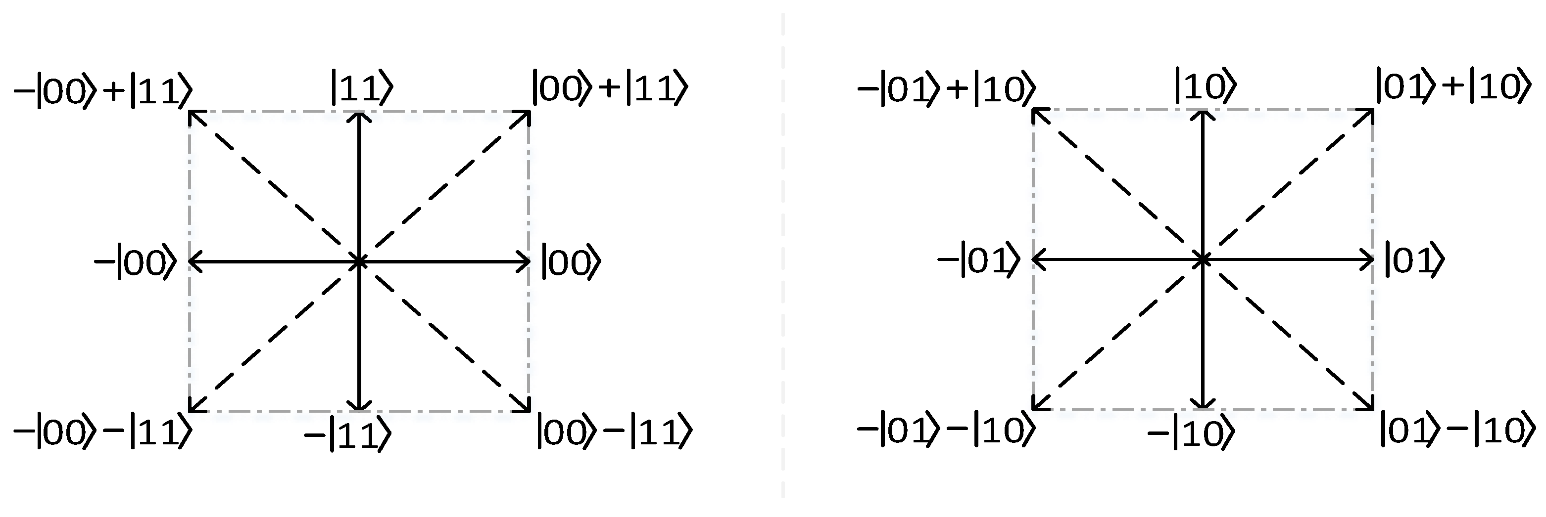
| (a) | (b) | ||||
| (c) | (d) | ||||
4. Discussion
5. Conclusion
References
- Nielsen, M. A., Chuang, I. L. Quantum Computation and Quantum Information[M]. Cambridge University Press, 2000.
- Schro¨dinger, E. Die gegenwa¨rtige Situation in der Quantenmechanik. Naturwissenschaften 1935, 23, 844–849. [Google Scholar] [CrossRef]
- Horodecki, R., Horodecki, P., Horodecki, M., Horodecki, K. (2007). Quantum entanglement. Review of Modern Physics 2007, 81(2), 865–942.
- Zukowski, M., Zeilinger, A., Horne, M. A., et al. “Event-ready-detectors” Bell experiment via entanglement swapping. Physical Review Letters 1993, 71, 4287. [CrossRef] [PubMed]
- Ji, Z. X., Fan, P. R., Zhang, H. G. (2022). Entanglement swapping for Bell states and Greenberger–Horne–Zeilinger states in qubit systems. 585, 126400.
- Zhang, H. G., Ji, Z. X., Wang, H. Z., et al. (2019). Survey on quantum information security. China Communications 2019, 16(10), 1–36. [CrossRef]
- Bennett, C. H., Brassard, G., Crépeau, C., et al. Teleporting an unknown quantum state via dual classical and Einstein-Podolsky-Rosen channels. Physical review letters 1993, 70, 1895. [CrossRef] [PubMed]
- Bose, S., Vedral, V., Knight, P. L. (1998). Multiparticle generalization of entanglement swapping. Physical Review A 1998, 57(2), 822. [CrossRef]
- Hardy, L., Song, D. D. (2000). Entanglement swapping chains for general pure states. Physical Review A 2000, 62(5), 052315. [CrossRef]
- Bouda, J., Buzˇek, V. (2001). Entanglement swapping between multi-qudit systems. Journal of Physics A: Mathematical and General 2001, 34, 4301–4311. [CrossRef]
- Karimipour, V., Bahraminasab, A., Bagherinezhad, S. (2002). Entanglement swapping of generalized cat states and secret sharing. Physical Review A 2002, 65.
- Sen, A., Sen, U., Brukner, Cˇ., Buzˇek, V., Z˙ukowski, M. (2005). Entanglement swapping of noisy states: A kind of superadditivity in nonclassicality. Physical Review A 2005, 72, 042310. [CrossRef]
- Roa, L., Mun˜oz, A., Gru˜ning, G. (2014). Entanglement swapping for X states demands threshold values. Physical Review A 2014, 89(6), 064301. [CrossRef]
- Kirby, B. T., Santra, S., Malinovsky, V. S., Brodsky, M. (2016). Entanglement swapping of two arbitrarily degraded entangled states. Physical Review A 2016, 94, 012336. [CrossRef]
- Bergou, J. A., Fields, D., Hillery, M., Santra, S., Malinovsky, V. S. (2021). Average concurrence and entanglement swapping. Physical Review A 2021, 104(2), 022425.
- Bell, J. S. (1964). On the Einstein Podolsky Rosen paradox. Physics Physique Fizika, 1964; 1, 195.
- Ji, Z. X., Fan, P. R., Zhang, H. G. (2020). Entanglement swapping theory and beyond. arXiv preprint arXiv: 2009.02555.
Disclaimer/Publisher’s Note: The statements, opinions and data contained in all publications are solely those of the individual author(s) and contributor(s) and not of MDPI and/or the editor(s). MDPI and/or the editor(s) disclaim responsibility for any injury to people or property resulting from any ideas, methods, instructions or products referred to in the content. |
© 2025 by the authors. Licensee MDPI, Basel, Switzerland. This article is an open access article distributed under the terms and conditions of the Creative Commons Attribution (CC BY) license (http://creativecommons.org/licenses/by/4.0/).


