Theoretical Foundations of Quantum Mechanics

1. Introduction

The establishment of quantum mechanics is undoubtedly one of the greatest progress made by human beings in exploring the mysteries of nature in recent hundreds of years. Unfortunately, after a century of exploration, the fundamental principles behind quantum mechanics phenomena, including quantum superposition and quantum entanglement, remain unsolved mysteries; In other words, although quantum mechanical phenomena can be described mathematically, no one can clearly explain the reasons behind these phenomena.

Quantum superposition, or superposition for short, is a peculiar quantum mechanics phenomenon, which indicates that a quantum system can be in multiple different states simultaneously [1]. The most common case is the superposition of two opposing states, and one of the most famous examples is “Schr$\ddot{\mathrm{o}}$dinger’s cat”, which can be vividly expressed as “a cat can be both alive and dead at the same time” [2].

Quantum entanglement, abbreviated as entanglement, is a quantum mechanics phenomenon built on superposition. In other words, the existence of superposition states is the prerequisite for the existence of entanglement. An entangled system is a composite of two or more subsystems, the properties of all subsystems are integrated into a holistic property, and the properties of each subsystem cannot be described separately, only the properties of the whole system can be described [1,3]. When one of the subsystems is observed, the state of the other subsystems will change immediately without any time delay, which is a shocking and unsettling phenomenon as it goes against human common sense [1].

Entanglement swapping is another quantum mechanics phenomenon, which is based on entanglement but further reveals the mystery of nature. Suppose that there are two or more entangled states that are independent of each other, and that some particles are selected from each of the entangled states, and then a joint quantum measurement is perform on them. In this way, the measured particles collapse into a new entangled state, while all unmeasured particles collapse into another new entangled state. This phenomenon is called entanglement swapping [4]. entanglement swapping is one of the core resources for preparing quantum repeaters, which makes long-distance quantum communication and large-scale quantum networks possible [3,4,5]; In addition, entanglement swapping provides a new approach for the preparation of entangled states and is also an important resource for designing quantum cryptography protocols and quantum algorithms [4,6,7].

It is not very difficult to mathematically characterize the basic situations of the aforementioned quantum mechanics phenomena; however, as mentioned earlier, it is very difficult to explain why such a characterization is possible. We believe that relying solely on scientific exploration can not find the ideal answer that can explain the principles of quantum mechanics, hence we turn our attention to ancient Chinese philosophy. Inspired by some theories in the I Ching and the Tao Te Ching, we in this paper combine the law of conservation of energy in classical physics with some existing principles of quantum mechanics to propose a theoretical framework, which can provide a new perspective for understanding quantum mechanical phenomena. Based on the proposed theoretical framework, we design a new algorithm for entanglement swapping. We demonstrate the algorithm through the entanglement swapping between two entangled states with two particles each, and then verify the correctness of the algorithm through the entanglement swapping between two Bell states (also commonly referred to as Einstein-Podolsky-Rosen pairs, abbreviated as EPR pairs [8]), in which the entanglement swapping is achieved by performing a Bell measurement on the first particle in each state.

In the following text, we will describe the proposed theoretical framework in Sec. 2. In Sec. 3, we will introduce several core theories in the I Ching and the Tao Te Ching, and elaborate on our viewpoints, which contributes to a better understanding of our proposed theoretical framework. In Sec. 4, we will first introduce the algebraic algorithm for entanglement swapping between two Bell states, then show our proposed algorithm. Finally, we make a summary in Sec. 5.

2. The Proposed Theoretical Framework

From classical physics theory, it is known that energy cannot appear out of thin air, and matter is no exception [9]. Obviously, at the beginning of the birth of the universe, there must have been nothing at all, that is, the origin of the universe was empty; In other words, the empty state is the starting state of the universe. However, the birth of infinite energy and countless kinds of substances in the universe indicates that the origin of the universe is all-encompassing; From this perspective, the all-encompassing state is the beginning state of the universe. By the way, as for how primitive energy emerged, it seems to me that there will probably never be an answer to this question.

To sum up, the origin of the universe is both “empty” and “all-embracing”, which can be said to be the superposition or mixture of the two opposing states. Using mathematical representations in quantum mechanics, we would like to represent the “empty state” and “all-embracing state” separately as $\left|\mathcal{N}\right.〉$ and $\left|\mathcal{Y}\right.〉$, and use $\left|\mathcal{O}\right.〉$ to represent the origin state of the universe, then one can get

$$\begin{array}{c}\hfill \left|\mathcal{O}\right.〉=\left|\mathcal{N}\right.〉+\left|\mathcal{Y}\right.〉.\end{array}$$

(1)

Furthermore, we can say that all things in the universe are the superposition of two opposite states, and their states can also be expressed in a form similar to the formula. For example, when we discuss or make a judgment about the existence of something, it is actually because we have made local observations of $\left|\mathcal{O}\right.〉$, which leads to its collapse, and thus we get the observation result $\left|\mathcal{Y}\right.〉$ or $\left|\mathcal{N}\right.〉$, where $\left|\mathcal{Y}\right.〉$ and $\left|\mathcal{N}\right.〉$ represent the two states of “existence” and “nonexistence”, respectively. Incidentally, due to local observations, our judgment is undoubtedly one-sided.

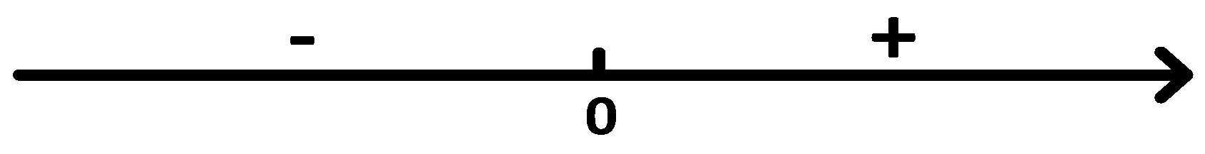
In the scientific community, it is generally believed that there is energy in the universe first, and then energy is transformed into various substances. However, the premise of accepting this viewpoint is that energy exists, that is, $\left|\mathcal{O}\right.〉$ is observed to collapse into the state $\left|\mathcal{Y}\right.〉$. As mentioned above, according to the law of conservation of energy, energy cannot be generated out of thin air, hence the total energy in the universe must be zero, which means that energy must be divided into positive energy and negative energy, and both are equal in quantity (that is, they are balanced), so as to ensure that the total energy is zero. Let us take the number axis as an example. The positive and negative energies correspond to the positive and negative half axes of the number axis, respectively, and the number 0 in the center of the number axis corresponds to the state after adding the two energies, as shown in Figure 1.

Figure 1.

Figure 1.

To further explore the state of the origin of the universe, let us assume that there is a quantum system that is always isolated from the outside world, which means that there has never been any energy exchange between the system and the external environment. As mentioned above, the energy possessed by the system includes positive energy and negative energy, and they are balanced. Here, we might as well use $\left|\phi \right.〉$ to represent the state of the system, and $\left|\alpha \right.〉$ and $\left|\beta \right.〉$ to represent the states of the positive and negative energy of the system, respectively, where $\left|\phi \right.〉$ can be assumed to be of any dimension. Without loss of generality, we would like to assume that $\left|\phi \right.〉$ is a d-dimensional quantum system (also often referred to as a d-level quantum system). Due to the energy of the system is zero, we can write it as

$$\begin{array}{c}\hfill \left|\phi \right.〉={\left(0,0,\dots ,0\right)}^{\mathrm{T}},\end{array}$$

(2)

that is, $\left|\phi \right.〉$ is a vector containing d zeros. Furthermore, let us represent $\left|\alpha \right.〉$ as

$$\begin{array}{c}\hfill \left|\alpha \right.〉={\left({\gamma }_1,{\gamma }_2,\dots ,{\gamma }_d\right)}^{\mathrm{T}}.\end{array}$$

(3)

Since the balance between the positive energy and negative energy, we have

$$\begin{array}{c}\hfill \left|\beta \right.〉={\left(-{\gamma }_1,-{\gamma }_2,\dots ,-{\gamma }_d\right)}^{\mathrm{T}}=-\left|\alpha \right.〉={\mathrm{e}}^{i\pi }\left|\alpha \right.〉.\end{array}$$

(4)

It is obvious that

$$\begin{array}{c}\hfill \left|\alpha \right.〉+\left|\beta \right.〉\equiv \left|\phi \right.〉.\end{array}$$

(5)

When conducting local observations on the system (i.e., performing quantum measurements on $\left|\alpha \right.〉$ or $\left|\beta \right.〉$), based on the theory of quantum measurements, only the state $\left|\alpha \right.〉$ can be obtained, attributed to

$$\begin{array}{c}\hfill \left.〈\beta \right|M_m^{+}{M}_m\left|\beta \right.〉=\left.〈\alpha \right|{\mathrm{e}}^{-i\pi }{M}_m^{+}{M}_m{\mathrm{e}}^{i\pi }\left|\alpha \right.〉=\left.〈\alpha \right|M_m^{+}{M}_m\left|\alpha \right.〉,\end{array}$$

(6)

where $M_m$ represents a measurement operator with m as the indicator [1]. Obviously, when the observation result is $\left|\alpha \right.〉$, the original state of the system is the superposition of $\left|\alpha \right.〉$ and $\left|\beta \right.〉$ (i.e., $-\left|\alpha \right.〉$), which is an interesting and shocking phenomenon. More precisely, since the probability of the observation result being either $\left|\alpha \right.〉$ or $\left|\beta \right.〉$ is 50% (they are balanced), we can denote the system $\left|\phi \right.〉$ as

$$\begin{array}{c}\hfill \left|\phi \right.〉={\displaystyle \frac{1}{\sqrt{2}}}\left(\left|\alpha \right.〉+\left|\beta \right.〉\right).\end{array}$$

(7)

In what follows, let us delve into $\left|\alpha \right.〉$ in more detail. Assuming that the states $\left|\xi \right.〉$ and $\left|\overline{\xi }\right.〉$ can be observed from $\left|\alpha \right.〉$, then we might as well denote $\left|\alpha \right.〉$ as

$$\begin{array}{c}\left|\alpha \right.〉={\eta }_1\left|\xi \right.〉+{\eta }_2\left|\overline{\xi }\right.〉,\\ \mathrm{s}.\mathrm{t}.{∥{\eta }_1∥}^2+{∥{\eta }_2∥}^2=1.\end{array}$$

(8)

In fact, it is well known that a quantum system in the real world cannot be completely isolated from the outside world, thus there must be energy exchange with the external environment, meaning that there is an increase or decrease of positive energy and negative energy, which often makes them unbalanced. In this case, the coefficients ${\eta }_1$ and ${\eta }_2$ in the above equation are often not equal. Nonetheless, we focus our attention on the observation results rather than the coefficients, for the sake of simplicity, we would like to set ${\eta }_1={\eta }_2={\displaystyle \frac{1}{\sqrt{2}}}$, such that $\left|\alpha \right.〉={\displaystyle \frac{1}{\sqrt{2}}}\left(\left|\xi \right.〉+\left|\overline{\xi }\right.〉\right)$. Then we have

$$\begin{array}{cc}\hfill \left|\phi \right.〉=& {\displaystyle \frac{1}{\sqrt{2}}}\left(\left|\alpha \right.〉+\left|\beta \right.〉\right)\hfill \\ \hfill =& {\displaystyle \frac{1}{\sqrt{2}}}\left\{{\displaystyle \frac{1}{\sqrt{2}}}\left(\left|\xi \right.〉+\left|\overline{\xi }\right.〉\right)+\left[-{\displaystyle \frac{1}{\sqrt{2}}}\left(\left|\xi \right.〉+\left|\overline{\xi }\right.〉\right)\right]\right\}\hfill \\ \hfill =& {\displaystyle \frac{1}{\sqrt{2}}}\left\{{\displaystyle \frac{1}{\sqrt{2}}}\left(\left|\xi \right.〉-\left|\overline{\xi }\right.〉\right)+\left[-{\displaystyle \frac{1}{\sqrt{2}}}\left(\left|\xi \right.〉-\left|\overline{\xi }\right.〉\right)\right]\right\}\hfill \\ \hfill =& {\displaystyle \frac{1}{2}}\left[\left|\xi \right.〉+\left(-\left|\xi \right.〉\right)\right]+{\displaystyle \frac{1}{2}}\left[\left|\overline{\xi }\right.〉+\left(-\left|\overline{\xi }\right.〉\right)\right].\hfill \end{array}$$

(9)

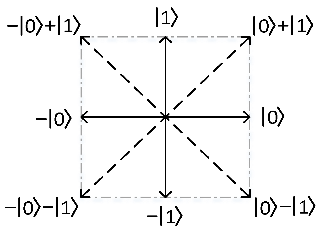
As can be seen from Eq. 9, in addition to $\left|\xi \right.〉$, the states $\left|\overline{\xi }\right.〉$, ${\displaystyle \frac{1}{\sqrt{2}}}\left(\left|\xi \right.〉+\left|\overline{\xi }\right.〉\right)$ and ${\displaystyle \frac{1}{\sqrt{2}}}\left(\left|\xi \right.〉-\left|\overline{\xi }\right.〉\right)$ can be observed from the system $\left|\phi \right.〉$, which is undoubtedly an interesting and shocking phenomenon. Indeed, to be precise, countless states can be observed from $\left|\phi \right.〉$, and the observed states are entirely determined by measurement operators. Let us give a few familiar examples. Assuming that $\left|\alpha \right.〉$ is in the state $\left|+\right.〉={\displaystyle \frac{1}{\sqrt{2}}}\left(\left|0\right.〉+\left|1\right.〉\right)$, then one can get

$$\begin{array}{cc}\hfill \left|\phi \right.〉=& {\displaystyle \frac{1}{\sqrt{2}}}\left\{{\displaystyle \frac{1}{\sqrt{2}}}\left(\left|0\right.〉+\left|1\right.〉\right)+\left[-{\displaystyle \frac{1}{\sqrt{2}}}\left(\left|0\right.〉+\left|1\right.〉\right)\right]\right\}\hfill \\ \hfill =& {\displaystyle \frac{1}{\sqrt{2}}}\left\{{\displaystyle \frac{1}{\sqrt{2}}}\left(\left|0\right.〉-\left|1\right.〉\right)+\left[-{\displaystyle \frac{1}{\sqrt{2}}}\left(\left|0\right.〉-\left|1\right.〉\right)\right]\right\}\hfill \\ \hfill =& {\displaystyle \frac{1}{2}}\left[\left|0\right.〉+\left(-\left|0\right.〉\right)\right]+{\displaystyle \frac{1}{2}}\left[\left|1\right.〉+\left(-\left|1\right.〉\right)\right].\hfill \end{array}$$

(10)

It can be seen that there are four states that can be observed from the system $\left|\phi \right.〉$, as follows:

$$\begin{array}{c}\hfill \left|0\right.〉,\left|1\right.〉,\left|+\right.〉,\left|-\right.〉,\end{array}$$

(11)

where $\left|-\right.〉={\displaystyle \frac{1}{\sqrt{2}}}\left(\left|0\right.〉-\left|1\right.〉\right)$. In other words, if the system is observed locally, the four states shown in Eq. 11 can be observed. Treating $\left|0\right.〉$ and $\left|1\right.〉$ as vectors, we can establish a coordinate system as shown in Figure 2. Note here that the global phase of each state in the figure is artificially specified, not constant (similarly hereinafter). For example, for the states in the horizontal direction, the vector to the right is specified to be $\left|0\right.〉$ and the vector to the left is $-\left|0\right.〉$; Of course, the reverse can be specified, that is, swapping the positions of $\left|0\right.〉$ and $-\left|0\right.〉$ is also possible. We adopt the regulations shown in Figure 2 only out of habit.

Figure 2.

Figure 2.

Next, let us consider the case of conducting local observations on two quantum systems. To study this problem, let us assume that there are two independent quantum systems, $\left|{\Psi }_1\right.〉$ and $\left|{\Psi }_2\right.〉$, in the states of

$$\begin{array}{cc}\hfill & \left|{\Psi }_1\right.〉={\displaystyle \frac{1}{\sqrt{2}}}\left\{{\displaystyle \frac{1}{\sqrt{2}}}\left(\left|u_1\right.〉+\left|{\overline{u}}_1\right.〉\right)+\left[-{\displaystyle \frac{1}{\sqrt{2}}}\left(\left|u_1\right.〉+\left|{\overline{u}}_1\right.〉\right)\right]\right\},\hfill \\ \hfill & \left|{\Psi }_2\right.〉={\displaystyle \frac{1}{\sqrt{2}}}\left\{{\displaystyle \frac{1}{\sqrt{2}}}\left(\left|u_2\right.〉+\left|{\overline{u}}_2\right.〉\right)+\left[-{\displaystyle \frac{1}{\sqrt{2}}}\left(\left|u_2\right.〉+\left|{\overline{u}}_2\right.〉\right)\right]\right\},\hfill \end{array}$$

(12)

where $\left\{\left|u_1\right.〉,\left|{\overline{u}}_1\right.〉\right\}$ and $\left\{\left|u_2\right.〉,\left|{\overline{u}}_2\right.〉\right\}$ are the observation results of $\left|{\Psi }_1\right.〉$ and $\left|{\Psi }_2\right.〉$, respectively. Then we can get

$$\begin{array}{cc}\hfill & \left|{\Psi }_1\right.〉\otimes \left|{\Psi }_2\right.〉\hfill \\ \hfill =& {\displaystyle \frac{1}{\sqrt{2}}}\left\{{\displaystyle \frac{1}{\sqrt{2}}}\left(\left|u_1\right.〉+\left|{\overline{u}}_1\right.〉\right)+\left[-{\displaystyle \frac{1}{\sqrt{2}}}\left(\left|u_1\right.〉+\left|{\overline{u}}_1\right.〉\right)\right]\right\}\otimes {\displaystyle \frac{1}{\sqrt{2}}}\left\{{\displaystyle \frac{1}{\sqrt{2}}}\left(\left|u_2\right.〉+\left|{\overline{u}}_2\right.〉\right)+\left[-{\displaystyle \frac{1}{\sqrt{2}}}\left(\left|u_2\right.〉+\left|{\overline{u}}_2\right.〉\right)\right]\right\}\hfill \\ \hfill \Rightarrow & {\displaystyle \frac{1}{2\sqrt{2}}}\left\{\left(\left|u_1{u}_2\right.〉+\left|u_1{\overline{u}}_2\right.〉+\left|{\overline{u}}_1{u}_2\right.〉+\left|{\overline{u}}_1{\overline{u}}_2\right.〉\right)+\left[-\left(\left|u_1{u}_2\right.〉+\left|u_1{\overline{u}}_2\right.〉+\left|{\overline{u}}_1{u}_2\right.〉+\left|{\overline{u}}_1{\overline{u}}_2\right.〉\right)\right]\right\}\hfill \end{array}$$

(13a)

$$\begin{array}{cc}\hfill =& {\displaystyle \frac{1}{2}}\left\{{\displaystyle \frac{1}{\sqrt{2}}}\left(\left|u_1{u}_2\right.〉+\left|{\overline{u}}_1{\overline{u}}_2\right.〉\right)+\left[-{\displaystyle \frac{1}{\sqrt{2}}}\left(\left|u_1{u}_2\right.〉+\left|{\overline{u}}_1{\overline{u}}_2\right.〉\right)\right]\right\}\hfill \\ \hfill & +{\displaystyle \frac{1}{2}}\left\{{\displaystyle \frac{1}{\sqrt{2}}}\left(\left|u_1{\overline{u}}_2\right.〉+\left|{\overline{u}}_1{u}_2\right.〉\right)+\left[-{\displaystyle \frac{1}{\sqrt{2}}}\left(\left|u_1{\overline{u}}_2\right.〉+\left|{\overline{u}}_1{u}_2\right.〉\right)\right]\right\}\hfill \end{array}$$

(13b)

$$\begin{array}{cc}\hfill =& {\displaystyle \frac{1}{2}}\left\{{\displaystyle \frac{1}{\sqrt{2}}}\left(\left|u_1{u}_2\right.〉-\left|{\overline{u}}_1{\overline{u}}_2\right.〉\right)+\left[-{\displaystyle \frac{1}{\sqrt{2}}}\left(\left|u_1{u}_2\right.〉-\left|{\overline{u}}_1{\overline{u}}_2\right.〉\right)\right]\right\}\hfill \\ \hfill & +{\displaystyle \frac{1}{2}}\left\{{\displaystyle \frac{1}{\sqrt{2}}}\left(\left|u_1{\overline{u}}_2\right.〉-\left|{\overline{u}}_1{u}_2\right.〉\right)+\left[-{\displaystyle \frac{1}{\sqrt{2}}}\left(\left|u_1{\overline{u}}_2\right.〉-\left|{\overline{u}}_1{u}_2\right.〉\right)\right]\right\}.\hfill \end{array}$$

(13c)

Note here that the second step in the above equation has undergone probability normalization. From Eqs. 13a, 13b and 13c, it can be seen that the following states can be observed from the composite system $\left|{\Psi }_1\right.〉\otimes \left|{\Psi }_2\right.〉$:

$$\begin{array}{c}\left\{\left|u_1{u}_2\right.〉,\left|u_1{\overline{u}}_2\right.〉,\left|{\overline{u}}_1{u}_2\right.〉,\left|{\overline{u}}_1{\overline{u}}_2\right.〉\right\},\\ \left\{\left|{\chi }_1\right.〉,\left|{\chi }_2\right.〉,\left|{\chi }_3\right.〉,\left|{\chi }_4\right.〉\right\},\\ \mathrm{where}\left|{\chi }_1\right.〉={\displaystyle \frac{1}{\sqrt{2}}}\left(\left|u_1{u}_2\right.〉+\left|{\overline{u}}_1{\overline{u}}_2\right.〉\right),\left|{\chi }_2\right.〉={\displaystyle \frac{1}{\sqrt{2}}}\left(\left|u_1{u}_2\right.〉-\left|{\overline{u}}_1{\overline{u}}_2\right.〉\right),\\ \left|{\chi }_3\right.〉={\displaystyle \frac{1}{\sqrt{2}}}\left(\left|u_1{\overline{u}}_2\right.〉+\left|{\overline{u}}_1{u}_2\right.〉\right),\left|{\chi }_4\right.〉={\displaystyle \frac{1}{\sqrt{2}}}\left(\left|u_1{\overline{u}}_2\right.〉-\left|{\overline{u}}_1{u}_2\right.〉\right).\end{array}$$

(14)

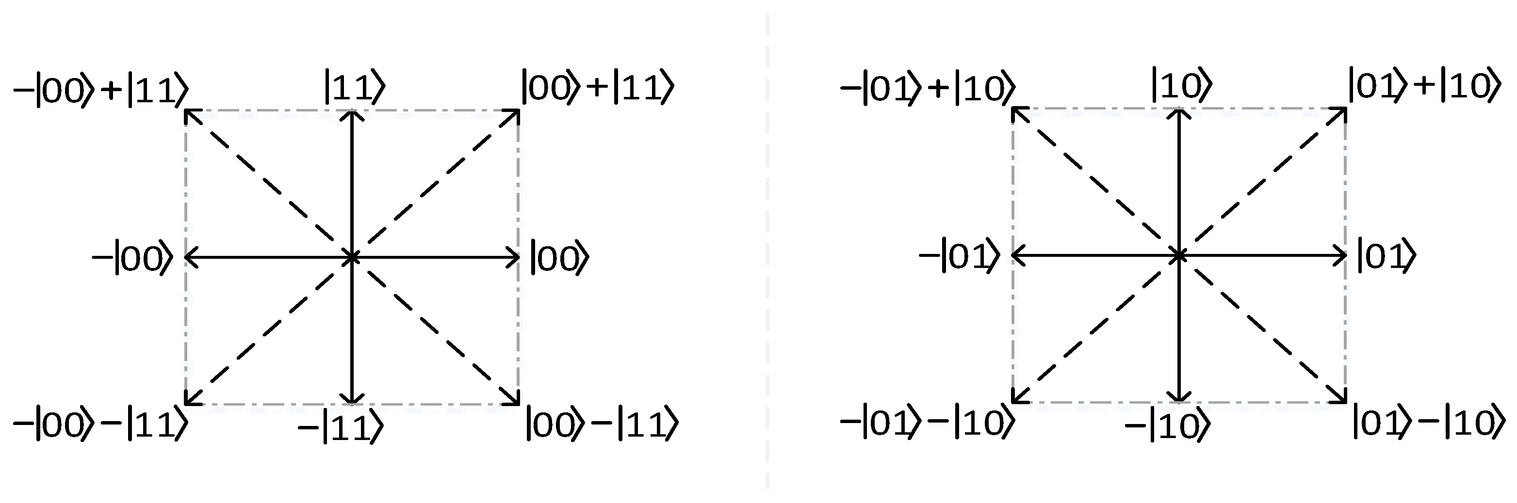
A familiar example is when $u_1\in \{0,1\},{\overline{u}}_1\in \{0,1\}\setminus \left\{u_1\right\}$ and $u_2\in \{0,1\},{\overline{u}}_2\in \{0,1\}\setminus \left\{u_2\right\}$, one can observe the following states:

$$\begin{array}{c}\left\{\left|00\right.〉,\left|01\right.〉,\left|10\right.〉,\left|11\right.〉\right\},\\ \left\{\left|{\varphi }^{+}\right.〉,\left|{\varphi }^{-}\right.〉,\left|{\psi }^{+}\right.〉,\left|{\psi }^{-}\right.〉\right\},\end{array}$$

(15)

where $\left|{\varphi }^{+}\right.〉,\left|{\varphi }^{-}\right.〉,\left|{\psi }^{+}\right.〉,\left|{\psi }^{-}\right.〉$ are Bell states (see Eq. 19). This example shows a surprising result, which may explain why Bell states exist in nature. Of course, as before, countless types of quantum states can be observed from $\left|{\Psi }_1\right.〉\otimes \left|{\Psi }_2\right.〉$, which will not be elaborated here. By the way, two coordinate systems can be established, as shown in Figure 3.

Figure 3.

Figure 3.

3. Discussion

From the law of conservation of energy, it is known that energy is constantly transforming or transferring, meaning that positive and negative energy in the universe are continuously converting into each other. Since the total energy in the universe is always zero, when a certain amount of positive energy is converted into negative energy, there must simultaneously be an equal amount of negative energy converted into positive energy. In short, the two are antagonistic, coexisting, balanced, and constantly transforming into each other, which is completely consistent with the Yin-Yang theory in the I Ching (also called the “Book of Changes”) [10]: Yin and Yang are opposing, coexisting, balanced and mutually transforming, where Yin and Yang refer to two opposing things, respectively, such as positive energy and negative energy, the wave and particle nature of light, continuous signals and discrete signals, etc.

As mentioned above, the existence of Yin and Yang is due to local observations, that is, the existence of any two opposing matter is the result of local observations. If Yin and Yang are balanced and a holistic observation can be made, the result would be “emptiness” (“void” or “nothingness”), which may validate the Buddhist idea that everything is empty. Due to the quantization of energy, we hold the opinion that the sense organs on human bodies are essentially quantum measuring instruments, while human beings are programmed, emotional, and self-aware “intelligent robots”, and our observations and judgments depend on the database in the “brain”. Specifically, we measure the received energy through our physical senses (quantum measuring instruments), then analyze and process the measurement results based on the data in our own database, and finally make actions such as judgments or feedback.

In short, the origin of the universe is like Doraemon’s pocket, which looks empty, but can take out anything that one wants. Through local observations of “emptiness”, people observe the existence of infinite positive and negative energy, and believe that energy is transformed into countless and diverse substances, which is consistent with the statement of Tao Te Ching [10]: all things in the world are born of existence, and existence is born of nothingness. People may ask: What is the state of “emptiness" and what force created it? In Tao Te Ching, it is stated that “Tao gives birth to one, one gives birth to two, two gives birth to three, and three gives birth to everything”. Therefore, the answer we find is that the “Tao” gives birth to “emptiness”. Here, “one” is “emptiness”, corresponding to the state $\left|\phi \right.〉$ in Eq. 7, while “two” refers to the positive and negative energy (if referred to as Yin and Yang, it would be more general), plus the state after the fusion of positive and negative energy, there is “three”.

Tao Te Ching states that the “Tao” is unknowable and unspeakable, and one possible important reason, we believe, is that humans are unable to observe the universe as a whole, but only small parts. For example, if we live in a virtual world created for us by a quantum computer with infinite computing power, we will never know what this computer looks like. In other words, the fundamental and eternal principles followed by the evolution of all things in the universe are unknowable and indescribable. On the contrary, the truth that can be explained clearly is definitely not eternal (these so-called truths are merely the truths put forward and recognized by people), as stated in Tao Te Ching: The principle that can be spoken is not the eternal principle. Based on this point, the truths that can be clearly articulated are not the ultimate truth.

According to the principle of Yin-yang balance, a clear explanation is equivalent to an unclear explanation. In other words, the more clearly we can describe a state, the greater the gap between it and the original state of things. On the contrary, if the state of a thing is more difficult to describe, then this state is more likely to be close to the real state of the thing. As mentioned earlier, it is difficult to describe the state formed by the mixing of two opposite states, yet this state is the most authentic. By the way, regarding the theoretical framework proposed in this article, if you find the framework very clear and you understand it, it also indicates that you do not understand it.

4. The New Algorithm for Entanglement Swapping

The original idea of entanglement swapping was included in the quantum teleportation scheme proposed by Bennett et al. in 1992 [11]. Soon afterwards, Zeilinger et al. experimentally realised entanglement swapping for the first time, and formally proposed the concept of entanglement swapping [5]. Subsequently, Bose et al. formulated the entanglement swapping of 2-level cat states [12]. Hardy and Song characterized the entanglement swapping of general pure states [13]. Bouda and Bu$\check{\mathrm{z}}$ek generalized the entanglement swapping case for two qudit systems to the case of multiple qudit systems [14]. Karimipour et al. introduced generalized cat states in d-level systems and derived the formulas of the entanglement swapping between d-level cat states and d-level Bell states [15]. Sen et al. investigated various entanglement swapping schemes for Werner states [16]. Roa et al. studied the entanglement swapping of X states [17]. Kirby et al. proposed a general analytical solution for entanglement swapping of arbitrary two-qubit states, which provides a comprehensive method for analyzing entanglement swapping in quantum networks [18]. Recently, Bergou et al. investigated the connection between entanglement swapping and concurrence [19].

In what follows, we will provide a detailed description of the proposed algorithm for entanglement swapping. Before that, let us first introduce the entanglement swapping between two Bell states.

4.1. Entanglement Swapping Between Two Bell States

The algebraic calculation process of entanglement swapping can be simply described as the expansion of a polynomial composed of vectors, combining like terms, permutation, followed by the re-expansion of the polynomial, and then combining like terms [20]. In what follows, we will introduce the entanglement swapping between two Bell states. Bell states contains four different states, which can be denoted as [20]

$$\begin{array}{c}\left|\phi \left({\lambda }_1,{\lambda }_2\right)\right.〉={\displaystyle \frac{1}{\sqrt{2}}}{\left[\left|0{\lambda }_2\right.〉+{(-1)}^{{\lambda }_1}\left|1{\overline{\lambda }}_2\right.〉\right]}_{1,2},\\ {\lambda }_1,{\lambda }_2\in \{0,1\},\end{array}$$

(16)

where the subscripts 1,2 denote the two particles in each state (similarly hereinafter). It is known that four Bell states form a complete orthogonal basis, i.e., the Bell basis [4], which are widely used as measurement operators to extract information carried on entangled states or for realizing entanglement swapping.

Let us suppose that there are two Bell states, denoted as ${\left|\phi \left({\lambda }_1^1,{\lambda }_2^1\right)\right.〉}_{1,2}$ and ${\left|\phi \left({\lambda }_1^2,{\lambda }_2^2\right)\right.〉}_{3,4}$, where the subscripts 1,2 and 3,4 denote the particles in the two Bell states, respectively, and suppose that a Bell measurement is performed on the first particle in each state, such that the entanglement swapping between two Bell states can be expressed as [20]

$$\begin{array}{cc}\hfill & {\left|\phi \left({\lambda }_1^1,{\lambda }_2^1\right)\right.〉}_{1,2}\otimes {\left|\phi \left({\lambda }_1^2,{\lambda }_2^2\right)\right.〉}_{3,4}\hfill \\ \hfill =& {\displaystyle \frac{1}{2}}{\left[\left|0{\lambda }_2^{1}0{\lambda }_2^2\right.〉+{(-1)}^{{\lambda }_1^2}\left|0{\lambda }_2^{1}1{\overline{\lambda }}_2^2\right.〉+{(-1)}^{{\lambda }_1^1}\left|1{\overline{\lambda }}_2^{1}0{\lambda }_2^2\right.〉+{(-1)}^{{\lambda }_1^1+{\lambda }_1^2}\left|1{\overline{\lambda }}_2^{1}1{\overline{\lambda }}_2^2\right.〉\right]}_{1234}\hfill \end{array}$$

(17a)

$$\begin{array}{c}\hfill \Rightarrow {\displaystyle \frac{1}{2}}{\left[\left|00{\lambda }_2^1{\lambda }_2^2\right.〉+{(-1)}^{{\lambda }_1^2}\left|01{\lambda }_2^1{\overline{\lambda }}_2^2\right.〉+{(-1)}^{{\lambda }_1^1}\left|10{\overline{\lambda }}_2^1{\lambda }_2^2\right.〉+{(-1)}^{{\lambda }_1^1+{\lambda }_1^2}\left|11{\overline{\lambda }}_2^1{\overline{\lambda }}_2^2\right.〉\right]}_{1324}\end{array}$$

(17b)

$$\begin{array}{cc}\hfill =& {\displaystyle \frac{1}{4}}\left[1+{(-1)}^{{\lambda }_1^1+{\lambda }_1^2}\right]\left(\left|\phi \left(0,0\right)\right.〉\left|\phi \left(0,{\lambda }_1^2\right)\right.〉\pm \left|\phi \left(1,0\right)\right.〉\left|\phi \left(1,{\overline{\lambda }}_1^2\right)\right.〉\right)\hfill \\ \hfill +& {\displaystyle \frac{1}{4}}\left[1-{(-1)}^{{\lambda }_1^1+{\lambda }_1^2}\right]\left(\left|\phi \left(1,0\right)\right.〉\left|\phi \left(0,{\lambda }_1^2\right)\right.〉\pm \left|\phi \left(0,0\right)\right.〉\left|\phi \left(1,{\overline{\lambda }}_1^2\right)\right.〉\right)\hfill \\ \hfill +& {\displaystyle \frac{1}{4}}\left[{(-1)}^{{\lambda }_1^2}+{(-1)}^{{\lambda }_1^1}\right]\left(\left|\phi \left(0,1\right)\right.〉\left|\phi \left(0,{\lambda }_2^2\right)\right.〉\pm \left|\phi \left(1,1\right)\right.〉\left|\phi \left(1,{\overline{\lambda }}_2^2\right)\right.〉\right)\hfill \\ \hfill +& {\displaystyle \frac{1}{4}}\left[{(-1)}^{{\lambda }_1^2}-{(-1)}^{{\lambda }_1^1}\right]\left(\left|\phi \left(1,1\right)\right.〉\left|\phi \left(0,{\lambda }_2^2\right)\right.〉\pm \left|\phi \left(0,1\right)\right.〉\left|\phi \left(1,{\overline{\lambda }}_2^2\right)\right.〉\right).\hfill \end{array}$$

(17c)

This formula demonstrates a detailed algebraic calculation process for deriving entanglement swapping results. Eq. 17a shows the result after the expansion of polynomials and the merging of similar terms; Eq. 17b shows the result after permutation; Eq. 17c shows the result after the re-expansion of the polynomial and the combining of like terms.

Ref. [4] provides another expression for entanglement swapping between two Bell states, which are given by

$$\begin{array}{cc}\hfill & {\left(\left|0i\right.〉\pm \left|1\overline{i}\right.〉\right)}_{12}\otimes {\left(\left|0i\right.〉\pm \left|1\overline{i}\right.〉\right)}_{34}\hfill \\ \hfill \Rightarrow & \left\{\begin{array}{cc}\hfill & {\left|{\varphi }^{+}\right.〉}_{13}{\left|{\varphi }^{+}\right.〉}_{24}+{\left|{\varphi }^{-}\right.〉}_{13}{\left|{\varphi }^{-}\right.〉}_{24}\pm {\left|{\psi }^{+}\right.〉}_{13}{\left|{\psi }^{+}\right.〉}_{24}\pm {\left|{\psi }^{-}\right.〉}_{13}{\left|{\psi }^{-}\right.〉}_{24}\mathrm{if}\phantom{i}i=0;\hfill \\ \hfill & {\left|{\varphi }^{+}\right.〉}_{13}{\left|{\varphi }^{+}\right.〉}_{24}-{\left|{\varphi }^{-}\right.〉}_{13}{\left|{\varphi }^{-}\right.〉}_{24}\pm {\left|{\psi }^{+}\right.〉}_{13}{\left|{\psi }^{+}\right.〉}_{24}\mp {\left|{\psi }^{-}\right.〉}_{13}{\left|{\psi }^{-}\right.〉}_{24}\mathrm{if}\phantom{i}i=1,\hfill \end{array}\right.\hfill \end{array}$$

(18a)

$$\begin{array}{cc}\hfill & {\left(\left|0i\right.〉\pm \left|1\overline{i}\right.〉\right)}_{12}\otimes {\left(\left|0i\right.〉\mp \left|1\overline{i}\right.〉\right)}_{34}\hfill \\ \hfill \Rightarrow & \left\{\begin{array}{c}\phantom{-}{\left|{\varphi }^{+}\right.〉}_{13}{\left|{\varphi }^{-}\right.〉}_{24}+{\left|{\varphi }^{-}\right.〉}_{13}{\left|{\varphi }^{+}\right.〉}_{24}\mp {\left|{\psi }^{+}\right.〉}_{13}{\left|{\psi }^{-}\right.〉}_{24}\mp {\left|{\psi }^{-}\right.〉}_{13}{\left|{\psi }^{+}\right.〉}_{24}\mathrm{if}\phantom{i}i=0;\hfill \\ -{\left|{\varphi }^{+}\right.〉}_{13}{\left|{\varphi }^{-}\right.〉}_{24}+{\left|{\varphi }^{-}\right.〉}_{13}{\left|{\varphi }^{+}\right.〉}_{24}\pm {\left|{\psi }^{+}\right.〉}_{13}{\left|{\psi }^{-}\right.〉}_{24}\mp {\left|{\psi }^{-}\right.〉}_{13}{\left|{\psi }^{+}\right.〉}_{24}\mathrm{if}\phantom{i}i=1,\hfill \end{array}\right.\hfill \end{array}$$

(18b)

$$\begin{array}{cc}\hfill & {\left(\left|0i\right.〉\pm \left|1\overline{i}\right.〉\right)}_{12}\otimes {\left(\left|0\overline{i}\right.〉\pm \left|1i\right.〉\right)}_{34}\hfill \\ \hfill \Rightarrow & \left\{\begin{array}{cc}\hfill & {\left|{\varphi }^{+}\right.〉}_{13}{\left|{\psi }^{+}\right.〉}_{24}+{\left|{\varphi }^{-}\right.〉}_{13}{\left|{\psi }^{-}\right.〉}_{24}\pm {\left|{\psi }^{+}\right.〉}_{13}{\left|{\varphi }^{+}\right.〉}_{24}\pm {\left|{\psi }^{-}\right.〉}_{13}{\left|{\varphi }^{-}\right.〉}_{24}\mathrm{if}\phantom{i}i=0;\hfill \\ \hfill & {\left|{\varphi }^{+}\right.〉}_{13}{\left|{\psi }^{+}\right.〉}_{24}-{\left|{\varphi }^{-}\right.〉}_{13}{\left|{\psi }^{-}\right.〉}_{24}\pm {\left|{\psi }^{+}\right.〉}_{13}{\left|{\varphi }^{+}\right.〉}_{24}\mp {\left|{\psi }^{-}\right.〉}_{13}{\left|{\varphi }^{-}\right.〉}_{24}\mathrm{if}\phantom{i}i=1,\hfill \end{array}\right.\hfill \end{array}$$

(18c)

$$\begin{array}{cc}\hfill & {\left(\left|0i\right.〉\pm \left|1\overline{i}\right.〉\right)}_{12}\otimes {\left(\left|0\overline{i}\right.〉\mp \left|1i\right.〉\right)}_{34}\hfill \\ \hfill \Rightarrow & \left\{\begin{array}{c}\phantom{-}{\left|{\varphi }^{+}\right.〉}_{13}{\left|{\psi }^{-}\right.〉}_{24}+{\left|{\varphi }^{-}\right.〉}_{13}{\left|{\psi }^{+}\right.〉}_{24}\mp {\left|{\psi }^{+}\right.〉}_{13}{\left|{\varphi }^{-}\right.〉}_{24}\mp {\left|{\psi }^{-}\right.〉}_{13}{\left|{\varphi }^{+}\right.〉}_{24}\mathrm{if}\phantom{i}i=0;\hfill \\ -{\left|{\varphi }^{+}\right.〉}_{13}{\left|{\psi }^{-}\right.〉}_{24}+{\left|{\varphi }^{-}\right.〉}_{13}{\left|{\psi }^{+}\right.〉}_{24}\pm {\left|{\psi }^{+}\right.〉}_{13}{\left|{\varphi }^{-}\right.〉}_{24}\mp {\left|{\psi }^{-}\right.〉}_{13}{\left|{\varphi }^{+}\right.〉}_{24}\mathrm{if}\phantom{i}i=1,\hfill \end{array}\right.\hfill \end{array}$$

(18d)

where the inessential coefficients are ignored, and $\left|{\varphi }^{+}\right.〉,\left|{\varphi }^{-}\right.〉,\left|{\psi }^{+}\right.〉,\left|{\psi }^{-}\right.〉$ represent four Bell states, respectively, which can be denoted as

$$\begin{array}{c}\left|{\varphi }^{+}\right.〉={\displaystyle \frac{1}{\sqrt{2}}}\left(\left|00\right.〉+\left|11\right.〉\right),\left|{\varphi }^{-}\right.〉={\displaystyle \frac{1}{\sqrt{2}}}\left(\left|00\right.〉-\left|11\right.〉\right),\\ \left|{\psi }^{+}\right.〉={\displaystyle \frac{1}{\sqrt{2}}}\left(\left|01\right.〉+\left|10\right.〉\right),\left|{\psi }^{-}\right.〉={\displaystyle \frac{1}{\sqrt{2}}}\left(\left|01\right.〉-\left|10\right.〉\right).\end{array}$$

(19)

Eq. 19 is another way to characterize four Bell states besides Eq. 16, and this characterization is widely adopted in various quantum information processing tasks.

4.2. The Proposed Algorithm

From Eq. 13a, it can be seen that when $\left|u_1{u}_2\right.〉$ is obtained, the combination of the states of the two systems is $\left\{\left|u_1\right.〉,\left|u_2\right.〉\right\}$ or $\left\{-\left|u_1\right.〉,-\left|u_2\right.〉\right\}$. Furthermore, to obtain state $\left|{\chi }_1\right.〉$ (see Eq. 14), the state combinations of the two systems are the four combinations shown in Table 1, numbered ➀, ➁, ➂ and ➃. Similarly, the state combinations of the two systems can be derived when the states $\left|{\chi }_2\right.〉$, $\left|{\chi }_3\right.〉$ and $\left|{\chi }_4\right.〉$ are obtained, respectively, which will not be repeated here.

In what follows, let us introduce the new algorithm for deriving entanglement swapping results. For simplicity, we would only like to consider the entanglement swapping between two composite systems each containing two systems; Specifically, the entanglement swapping between two-particle entangled states (also known as bipartite entangled states). Of course, the algorithm is also applicable to multi-particle entangled states, since multi-particle states are just the generalization of two-particle states. Let us assume that there are two bipartite entangled states that are independent of the external environment and each other. Without loss of generality, let us represent the two states as ${\left|{\mathcal{A}}^{\pm }\right.〉}_{1,2}$ and ${\left|{\mathcal{B}}^{\pm }\right.〉}_{3,4}$, respectively, which are given by

$$\begin{array}{c}\hfill {\left|{\mathcal{A}}^{\pm }\right.〉}_{1,2}={\displaystyle \frac{1}{\sqrt{2}}}\left|a_1{a}_2\right.〉\pm {\displaystyle \frac{1}{\sqrt{2}}}\left|{\overline{a}}_1{\overline{a}}_2\right.〉,\\ \hfill {\left|{\mathcal{B}}^{\pm }\right.〉}_{3,4}={\displaystyle \frac{1}{\sqrt{2}}}\left|b_1{b}_2\right.〉\pm {\displaystyle \frac{1}{\sqrt{2}}}\left|{\overline{b}}_1{\overline{b}}_2\right.〉.\end{array}$$

(20)

Note here that the states $-{\left|{\mathcal{A}}^{\pm }\right.〉}_{1,2}$ and $-{\left|{\mathcal{B}}^{\pm }\right.〉}_{3,4}$ are ignored here, because the entangled states involved in entanglement swapping are obtained through observations (i.e., the states after the systems collapse), rather than the original states of the systems. By the way, the ignorance of $-{\left|{\mathcal{A}}^{\pm }\right.〉}_{1,2}$ and $-{\left|{\mathcal{B}}^{\pm }\right.〉}_{3,4}$ does not affect the correctness of the algorithm, and also makes the proposed algorithm look more concise.

Now, let us assume that the first particle in both ${\left|{\mathcal{A}}^{\pm }\right.〉}_{3,4}$ and ${\left|{\mathcal{B}}^{\pm }\right.〉}_{1,2}$ is observed simultaneously, and the observation result is denoted as ${\mathcal{M}}_1$, while the state that the remaining subsystems collapse onto is denoted as ${\mathcal{M}}_2$. In addition, we use the symbol $\mathcal{S}$ to represent the combinations of the states of the two particles. Indeed, the entanglement swapping between ${\left|{\mathcal{A}}^{\pm }\right.〉}_{1,2}$ and ${\left|{\mathcal{B}}^{\pm }\right.〉}_{3,4}$ include four cases: $\left\{{\left|{\mathcal{A}}^{+}\right.〉}_{1,2},{\left|{\mathcal{B}}^{+}\right.〉}_{3,4}\right\}$, $\left\{{\left|{\mathcal{A}}^{+}\right.〉}_{1,2},{\left|{\mathcal{B}}^{-}\right.〉}_{3,4}\right\}$, $\left\{{\left|{\mathcal{A}}^{-}\right.〉}_{1,2},{\left|{\mathcal{B}}^{+}\right.〉}_{3,4}\right\}$, and $\left\{{\left|{\mathcal{A}}^{-}\right.〉}_{1,2},{\left|{\mathcal{B}}^{-}\right.〉}_{3,4}\right\}$. For the first case, all the possible states of the particles and the corresponding observation results are listed in the four sub-tables in Table 2 (Note that for the sake of simplicity, unnecessary coefficients are ignored in the table.)

From the four sub-tables, we can summarize the following corresponding relationships:

$$\begin{array}{ccc}\hfill \left(a\right)& \left\{\begin{array}{c}\left(\left|a_1{b}_1\right.〉+\left|{\overline{a}}_1{\overline{b}}_1\right.〉,\left|a_2{b}_2\right.〉+\left|{\overline{a}}_2{\overline{b}}_2\right.〉\right),\hfill \\ \left(\left|a_1{\overline{b}}_1\right.〉+\left|{\overline{a}}_1{b}_1\right.〉,\left|a_2{\overline{b}}_2\right.〉+\left|{\overline{a}}_2{b}_2\right.〉\right),\hfill \end{array}\right.\left(b\right)\hfill & \hfill \left\{\begin{array}{c}\left(\left|a_1{b}_1\right.〉-\left|{\overline{a}}_1{\overline{b}}_1\right.〉,\left|a_2{b}_2\right.〉-\left|{\overline{a}}_2{\overline{b}}_2\right.〉\right),\hfill \\ \left(-\left|a_1{\overline{b}}_1\right.〉+\left|{\overline{a}}_1{b}_1\right.〉,-\left|a_2{\overline{b}}_2\right.〉+\left|{\overline{a}}_2{b}_2\right.〉\right),\hfill \end{array}\right.\\ \hfill \left(c\right)& \left\{\begin{array}{c}\left(\left|a_1{b}_1\right.〉-\left|{\overline{a}}_1{\overline{b}}_1\right.〉,\left|a_2{b}_2\right.〉-\left|{\overline{a}}_2{\overline{b}}_2\right.〉\right),\hfill \\ \left(\left|a_1{\overline{b}}_1\right.〉-\left|{\overline{a}}_1{b}_1\right.〉,\left|a_2{\overline{b}}_2\right.〉-\left|{\overline{a}}_2{b}_2\right.〉\right),\hfill \end{array}\right.\left(d\right)\hfill & \hfill \left\{\begin{array}{c}\left(\left|a_1{b}_1\right.〉+\left|{\overline{a}}_1{\overline{b}}_1\right.〉,\left|a_2{b}_2\right.〉+\left|{\overline{a}}_2{\overline{b}}_2\right.〉\right),\hfill \\ \left(-\left|a_1{\overline{b}}_1\right.〉-\left|{\overline{a}}_1{b}_1\right.〉,-\left|a_2{\overline{b}}_2\right.〉-\left|{\overline{a}}_2{b}_2\right.〉\right),\hfill \end{array}\right.\end{array}$$

(21)

then we can get the result of the entanglement swapping between ${\left|{\mathcal{A}}^{+}\right.〉}_{1,2}$ and ${\left|{\mathcal{B}}^{+}\right.〉}_{3,4}$,

$$\begin{array}{cc}\hfill {\left|{\mathcal{A}}^{+}\right.〉}_{1,2}\otimes {\left|{\mathcal{B}}^{+}\right.〉}_{3,4}⟶& \left(\left|a_1{b}_1\right.〉+\left|{\overline{a}}_1{\overline{b}}_1\right.〉\right)\otimes \left(\left|a_2{b}_2\right.〉+\left|{\overline{a}}_2{\overline{b}}_2\right.〉\right)\hfill \\ \hfill +& \left(\left|a_1{\overline{b}}_1\right.〉+\left|{\overline{a}}_1{b}_1\right.〉\right)\otimes \left(\left|a_2{\overline{b}}_2\right.〉+\left|{\overline{a}}_2{b}_2\right.〉\right)\hfill \\ \hfill +& \left(\left|a_1{b}_1\right.〉-\left|{\overline{a}}_1{\overline{b}}_1\right.〉\right)\otimes \left(\left|a_2{b}_2\right.〉-\left|{\overline{a}}_2{\overline{b}}_2\right.〉\right)\hfill \\ \hfill +& \left(\left|a_1{\overline{b}}_1\right.〉-\left|{\overline{a}}_1{b}_1\right.〉\right)\otimes \left(\left|a_2{\overline{b}}_2\right.〉-\left|{\overline{a}}_2{b}_2\right.〉\right).\hfill \end{array}$$

(22)

In a similar way, we can further obtain the results for other entangled swapping cases, which are given by

$$\begin{array}{cc}\hfill {\left|{\mathcal{A}}^{+}\right.〉}_{1,2}\otimes {\left|{\mathcal{B}}^{-}\right.〉}_{3,4}⟶& \left(\left|a_1{b}_1\right.〉+\left|{\overline{a}}_1{\overline{b}}_1\right.〉\right)\otimes \left(\left|a_2{b}_2\right.〉-\left|{\overline{a}}_2{\overline{b}}_2\right.〉\right)\hfill \\ \hfill -& \left(\left|a_1{\overline{b}}_1\right.〉+\left|{\overline{a}}_1{b}_1\right.〉\right)\otimes \left(\left|a_2{\overline{b}}_2\right.〉-\left|{\overline{a}}_2{b}_2\right.〉\right)\hfill \\ \hfill +& \left(\left|a_1{b}_1\right.〉-\left|{\overline{a}}_1{\overline{b}}_1\right.〉\right)\otimes \left(\left|a_2{b}_2\right.〉+\left|{\overline{a}}_2{\overline{b}}_2\right.〉\right)\hfill \\ \hfill -& \left(\left|a_1{\overline{b}}_1\right.〉-\left|{\overline{a}}_1{b}_1\right.〉\right)\otimes \left(\left|a_2{\overline{b}}_2\right.〉+\left|{\overline{a}}_2{b}_2\right.〉\right),\hfill \end{array}$$

(23)

$$\begin{array}{cc}\hfill {\left|{\mathcal{A}}^{-}\right.〉}_{1,2}\otimes {\left|{\mathcal{B}}^{+}\right.〉}_{3,4}⟶& \left(\left|a_1{b}_1\right.〉+\left|{\overline{a}}_1{\overline{b}}_1\right.〉\right)\otimes \left(\left|a_2{b}_2\right.〉-\left|{\overline{a}}_2{\overline{b}}_2\right.〉\right)\hfill \\ \hfill +& \left(\left|a_1{\overline{b}}_1\right.〉+\left|{\overline{a}}_1{b}_1\right.〉\right)\otimes \left(\left|a_2{\overline{b}}_2\right.〉-\left|{\overline{a}}_2{b}_2\right.〉\right)\hfill \\ \hfill +& \left(\left|a_1{b}_1\right.〉-\left|{\overline{a}}_1{\overline{b}}_1\right.〉\right)\otimes \left(\left|a_2{b}_2\right.〉+\left|{\overline{a}}_2{\overline{b}}_2\right.〉\right)\hfill \\ \hfill +& \left(\left|a_1{\overline{b}}_1\right.〉-\left|{\overline{a}}_1{b}_1\right.〉\right)\otimes \left(\left|a_2{\overline{b}}_2\right.〉+\left|{\overline{a}}_2{b}_2\right.〉\right),\hfill \end{array}$$

(24)

$$\begin{array}{cc}\hfill {\left|{\mathcal{A}}^{-}\right.〉}_{1,2}\otimes {\left|{\mathcal{B}}^{-}\right.〉}_{3,4}⟶& \left(\left|a_1{b}_1\right.〉+\left|{\overline{a}}_1{\overline{b}}_1\right.〉\right)\otimes \left(\left|a_2{b}_2\right.〉+\left|{\overline{a}}_2{\overline{b}}_2\right.〉\right)\hfill \\ \hfill -& \left(\left|a_1{\overline{b}}_1\right.〉+\left|{\overline{a}}_1{b}_1\right.〉\right)\otimes \left(\left|a_2{\overline{b}}_2\right.〉+\left|{\overline{a}}_2{b}_2\right.〉\right)\hfill \\ \hfill +& \left(\left|a_1{b}_1\right.〉-\left|{\overline{a}}_1{\overline{b}}_1\right.〉\right)\otimes \left(\left|a_2{b}_2\right.〉-\left|{\overline{a}}_2{\overline{b}}_2\right.〉\right)\hfill \\ \hfill -& \left(\left|a_1{\overline{b}}_1\right.〉-\left|{\overline{a}}_1{b}_1\right.〉\right)\otimes \left(\left|a_2{\overline{b}}_2\right.〉-\left|{\overline{a}}_2{b}_2\right.〉\right),\hfill \end{array}$$

(25)

If let $a_1,{\overline{a}}_1,a_2,{\overline{a}}_2,b_1,{\overline{b}}_1,b_2,{\overline{b}}_2\in \left\{0,1\right\}$, one can get the entanglement swapping between the Bell states, given by

$$\begin{array}{c}{\left|{\varphi }^{+}\right.〉}_{1,2}\otimes {\left|{\varphi }^{+}\right.〉}_{3,4}\to {\left|{\varphi }^{+}\right.〉}_{1,3}\otimes {\left|{\varphi }^{+}\right.〉}_{2,4}+{\left|{\varphi }^{-}\right.〉}_{1,3}\otimes {\left|{\varphi }^{-}\right.〉}_{2,4}+{\left|{\psi }^{+}\right.〉}_{1,3}\otimes {\left|{\psi }^{+}\right.〉}_{2,4}+{\left|{\psi }^{-}\right.〉}_{1,3}\otimes {\left|{\psi }^{-}\right.〉}_{2,4},\end{array}$$

(26a)

$$\begin{array}{c}{\left|{\varphi }^{+}\right.〉}_{1,2}\otimes {\left|{\psi }^{+}\right.〉}_{3,4}\to {\left|{\varphi }^{+}\right.〉}_{1,3}\otimes {\left|{\psi }^{+}\right.〉}_{2,4}+{\left|{\psi }^{+}\right.〉}_{1,3}\otimes {\left|{\varphi }^{+}\right.〉}_{2,4}+{\left|{\varphi }^{-}\right.〉}_{1,3}\otimes {\left|{\psi }^{-}\right.〉}_{2,4}+{\left|{\psi }^{-}\right.〉}_{1,3}\otimes {\left|{\varphi }^{-}\right.〉}_{2,4},\end{array}$$

(26b)

$$\begin{array}{c}{\left|{\psi }^{+}\right.〉}_{1,2}\otimes {\left|{\varphi }^{+}\right.〉}_{3,4}\to {\left|{\varphi }^{+}\right.〉}_{1,3}\otimes {\left|{\psi }^{+}\right.〉}_{2,4}+{\left|{\psi }^{+}\right.〉}_{1,3}\otimes {\left|{\varphi }^{+}\right.〉}_{2,4}-{\left|{\varphi }^{-}\right.〉}_{1,3}\otimes {\left|{\psi }^{-}\right.〉}_{2,4}-{\left|{\psi }^{-}\right.〉}_{1,3}\otimes {\left|{\varphi }^{-}\right.〉}_{2,4},\end{array}$$

(26c)

$$\begin{array}{c}{\left|{\psi }^{+}\right.〉}_{1,2}\otimes {\left|{\psi }^{+}\right.〉}_{3,4}\to {\left|{\varphi }^{+}\right.〉}_{1,3}\otimes {\left|{\varphi }^{+}\right.〉}_{2,4}+{\left|{\psi }^{+}\right.〉}_{1,3}\otimes {\left|{\psi }^{+}\right.〉}_{2,4}-{\left|{\varphi }^{-}\right.〉}_{1,3}\otimes {\left|{\varphi }^{-}\right.〉}_{2,4}-{\left|{\psi }^{-}\right.〉}_{1,3}\otimes {\left|{\psi }^{-}\right.〉}_{2,4},\end{array}$$

(26d)

$$\begin{array}{cc}\hfill & {\left|{\varphi }^{+}\right.〉}_{1,2}\otimes {\left|{\varphi }^{-}\right.〉}_{3,4}\to {\left|{\varphi }^{+}\right.〉}_{1,3}\otimes {\left|{\varphi }^{-}\right.〉}_{2,4}+{\left|{\varphi }^{-}\right.〉}_{1,3}\otimes {\left|{\varphi }^{+}\right.〉}_{2,4}-{\left|{\psi }^{+}\right.〉}_{1,3}\otimes {\left|{\psi }^{-}\right.〉}_{2,4}-{\left|{\psi }^{-}\right.〉}_{1,3}\otimes {\left|{\psi }^{+}\right.〉}_{2,4},\hfill \end{array}$$

(27a)

$$\begin{array}{cc}\hfill & {\left|{\varphi }^{+}\right.〉}_{1,2}\otimes {\left|{\psi }^{-}\right.〉}_{3,4}\to {\left|{\varphi }^{+}\right.〉}_{1,3}\otimes {\left|{\psi }^{-}\right.〉}_{2,4}-{\left|{\psi }^{+}\right.〉}_{1,3}\otimes {\left|{\varphi }^{-}\right.〉}_{2,4}+{\left|{\varphi }^{-}\right.〉}_{1,3}\otimes {\left|{\psi }^{+}\right.〉}_{2,4}-{\left|{\psi }^{-}\right.〉}_{1,3}\otimes {\left|{\varphi }^{+}\right.〉}_{2,4},\hfill \end{array}$$

(27b)

$$\begin{array}{cc}\hfill & {\left|{\psi }^{+}\right.〉}_{1,2}\otimes {\left|{\varphi }^{-}\right.〉}_{3,4}\to -{\left|{\varphi }^{+}\right.〉}_{1,3}\otimes {\left|{\varphi }^{-}\right.〉}_{2,4}+{\left|{\psi }^{+}\right.〉}_{1,3}\otimes {\left|{\varphi }^{-}\right.〉}_{2,4}+{\left|{\varphi }^{-}\right.〉}_{1,3}\otimes {\left|{\psi }^{+}\right.〉}_{2,4}-{\left|{\psi }^{-}\right.〉}_{1,3}\otimes {\left|{\varphi }^{+}\right.〉}_{2,4},\hfill \end{array}$$

(27c)

$$\begin{array}{cc}\hfill & {\left|{\psi }^{+}\right.〉}_{1,2}\otimes {\left|{\psi }^{-}\right.〉}_{3,4}\to -{\left|{\varphi }^{+}\right.〉}_{1,3}\otimes {\left|{\varphi }^{-}\right.〉}_{2,4}+{\left|{\psi }^{+}\right.〉}_{1,3}\otimes {\left|{\psi }^{-}\right.〉}_{2,4}+{\left|{\varphi }^{-}\right.〉}_{1,3}\otimes {\left|{\varphi }^{+}\right.〉}_{2,4}-{\left|{\psi }^{-}\right.〉}_{1,3}\otimes {\left|{\psi }^{+}\right.〉}_{2,4},\hfill \end{array}$$

(27d)

$$\begin{array}{cc}\hfill & {\left|{\varphi }^{-}\right.〉}_{1,2}\otimes {\left|{\varphi }^{+}\right.〉}_{3,4}\to {\left|{\varphi }^{+}\right.〉}_{1,3}\otimes {\left|{\varphi }^{-}\right.〉}_{2,4}+{\left|{\psi }^{+}\right.〉}_{1,3}\otimes {\left|{\psi }^{-}\right.〉}_{2,4}+{\left|{\varphi }^{-}\right.〉}_{1,3}\otimes {\left|{\varphi }^{+}\right.〉}_{2,4}+{\left|{\psi }^{-}\right.〉}_{1,3}\otimes {\left|{\psi }^{+}\right.〉}_{2,4},\hfill \end{array}$$

(28a)

$$\begin{array}{cc}\hfill & {\left|{\varphi }^{-}\right.〉}_{1,2}\otimes {\left|{\psi }^{+}\right.〉}_{3,4}\to {\left|{\varphi }^{+}\right.〉}_{1,3}\otimes {\left|{\psi }^{-}\right.〉}_{2,4}+{\left|{\psi }^{+}\right.〉}_{1,3}\otimes {\left|{\varphi }^{-}\right.〉}_{2,4}+{\left|{\varphi }^{-}\right.〉}_{1,3}\otimes {\left|{\psi }^{+}\right.〉}_{2,4}+{\left|{\psi }^{-}\right.〉}_{1,3}\otimes {\left|{\varphi }^{+}\right.〉}_{2,4},\hfill \end{array}$$

(28b)

$$\begin{array}{cc}\hfill & {\left|{\psi }^{-}\right.〉}_{1,2}\otimes {\left|{\varphi }^{+}\right.〉}_{3,4}\to -{\left|{\varphi }^{+}\right.〉}_{1,3}\otimes {\left|{\psi }^{-}\right.〉}_{2,4}-{\left|{\psi }^{+}\right.〉}_{1,3}\otimes {\left|{\varphi }^{-}\right.〉}_{2,4}+{\left|{\varphi }^{-}\right.〉}_{1,3}\otimes {\left|{\psi }^{+}\right.〉}_{2,4}+{\left|{\psi }^{-}\right.〉}_{1,3}\otimes {\left|{\varphi }^{+}\right.〉}_{2,4},\hfill \end{array}$$

(28c)

$$\begin{array}{cc}\hfill & {\left|{\psi }^{-}\right.〉}_{1,2}\otimes {\left|{\psi }^{+}\right.〉}_{3,4}\to -{\left|{\varphi }^{+}\right.〉}_{1,3}\otimes {\left|{\varphi }^{-}\right.〉}_{2,4}-{\left|{\psi }^{+}\right.〉}_{1,3}\otimes {\left|{\psi }^{-}\right.〉}_{2,4}+{\left|{\varphi }^{-}\right.〉}_{1,3}\otimes {\left|{\varphi }^{+}\right.〉}_{2,4}+{\left|{\psi }^{-}\right.〉}_{1,3}\otimes {\left|{\psi }^{+}\right.〉}_{2,4},\hfill \end{array}$$

(28d)

$$\begin{array}{cc}\hfill & {\left|{\varphi }^{-}\right.〉}_{1,2}\otimes {\left|{\varphi }^{-}\right.〉}_{3,4}\to {\left|{\varphi }^{+}\right.〉}_{1,3}\otimes {\left|{\varphi }^{+}\right.〉}_{2,4}-{\left|{\psi }^{+}\right.〉}_{1,3}\otimes {\left|{\psi }^{+}\right.〉}_{2,4}+{\left|{\varphi }^{-}\right.〉}_{1,3}\otimes {\left|{\varphi }^{-}\right.〉}_{2,4}-{\left|{\psi }^{-}\right.〉}_{1,3}\otimes {\left|{\psi }^{-}\right.〉}_{2,4},\hfill \end{array}$$

(29a)

$$\begin{array}{cc}\hfill & {\left|{\varphi }^{-}\right.〉}_{1,2}\otimes {\left|{\psi }^{-}\right.〉}_{3,4}\to {\left|{\varphi }^{+}\right.〉}_{1,3}\otimes {\left|{\psi }^{+}\right.〉}_{2,4}-{\left|{\psi }^{+}\right.〉}_{1,3}\otimes {\left|{\varphi }^{+}\right.〉}_{2,4}+{\left|{\varphi }^{-}\right.〉}_{1,3}\otimes {\left|{\psi }^{-}\right.〉}_{2,4}-{\left|{\psi }^{-}\right.〉}_{1,3}\otimes {\left|{\varphi }^{-}\right.〉}_{2,4},\hfill \end{array}$$

(29b)

$$\begin{array}{cc}\hfill & {\left|{\psi }^{-}\right.〉}_{1,2}\otimes {\left|{\varphi }^{-}\right.〉}_{3,4}\to {\left|{\varphi }^{+}\right.〉}_{1,3}\otimes {\left|{\psi }^{+}\right.〉}_{2,4}-{\left|{\psi }^{+}\right.〉}_{1,3}\otimes {\left|{\varphi }^{+}\right.〉}_{2,4}-{\left|{\varphi }^{-}\right.〉}_{1,3}\otimes {\left|{\psi }^{-}\right.〉}_{2,4}+{\left|{\psi }^{-}\right.〉}_{1,3}\otimes {\left|{\varphi }^{-}\right.〉}_{2,4},\hfill \end{array}$$

(29c)

$$\begin{array}{cc}\hfill & {\left|{\psi }^{-}\right.〉}_{1,2}\otimes {\left|{\psi }^{-}\right.〉}_{3,4}\to {\left|{\varphi }^{+}\right.〉}_{1,3}\otimes {\left|{\varphi }^{+}\right.〉}_{2,4}-{\left|{\psi }^{+}\right.〉}_{1,3}\otimes {\left|{\psi }^{+}\right.〉}_{2,4}-{\left|{\varphi }^{-}\right.〉}_{1,3}\otimes {\left|{\varphi }^{-}\right.〉}_{2,4}+{\left|{\psi }^{-}\right.〉}_{1,3}\otimes {\left|{\psi }^{-}\right.〉}_{2,4},\hfill \end{array}$$

(29d)

It can be seen that the cases shown in Eqs. (26a, 26d, 29a, 29d) are included in Eq. 18a; Eqs. (27a, 27d, 28a, 28d) are included in Eq. 18b; Eqs. (26b, 26c, 29b, 29c) are included in Eq. 18c; and Eqs. (27b, 27c, 28b, 28c) are included in Eq. 18d. In this way, the correctness of the algorithm is verified.

5. Conclusion

We have combined the law of conservation of energy with the principles of quantum mechanics to propose a theoretical framework, and designed a new algorithm for entanglement swapping based on the framework. We demonstrated the computation process of the algorithm through the entanglement swapping between two bipartite entangled states, and verified its correctness through the entanglement swapping of two Bell states. Our work provides new ideas and perspectives for studying the principles of quantum mechanics and exploring the mysteries of nature. Unfortunately, if the universe is seen as a composite system containing countless subsystems, then one can only observe a small subset of all the subsystems but not the entire system, thus cannot know the truth. A very unsettling question is: What force created the fundamental rules that govern the operation of all things in the universe?

References

- Nielsen, M. A., Chuang, I. L. Quantum Computation and Quantum Information. Cambridge University Press, 2000.
- Schro¨dinger, E. (1935). Die gegenwa¨rtige Situation in der Quantenmechanik. Naturwissenschaften, 23(50), 844-849.
- Horodecki, R., Horodecki, P., Horodecki, M., Horodecki, K. (2007). Quantum entanglement. Review of Modern Physics, 81(2), 865-942. [CrossRef]
- Ji, Z. X., Fan, P. R., Zhang, H. G. (2022). Entanglement swapping for Bell states and Greenberger–Horne–Zeilinger states in qubit systems. Physica A: Statistical Mechanics and its Applications, 585, 126400. [CrossRef]
- Zukowski, M., Zeilinger, A., Horne, M. A., et al. “Event-ready-detectors” Bell experiment via entanglement swapping. Physical Review Letters, 1993, 71(26), 4287. [CrossRef]
- Zhang, H. G., Ji, Z. X., Wang, H. Z., et al. (2019). Survey on quantum information security. China Communications, 16(10), 1-36. [CrossRef]
- Ji, Z. X., Fan, P. R., Zhang, H. G. (2020) Security proof of qudit-system-based quantum cryptography against entanglement-measurement attack. arXiv preprint, arXiv: 2012.14275. [CrossRef]
- Bell, J. S. (1964). On the Einstein Podolsky Rosen paradox. Physics Physique Fizika, 1(3), 195.
- Halliday, D., Resnick, R., Walker, J. Fundamentals of Physics[M]. Wiley, 2013.
- Zeng, S. Q., Liu, J. Z. The I Ching is really easy. Shaanxi Normal University Press, 2009.
- Bennett, C. H., Brassard, G., Crépeau, C., et al. Teleporting an unknown quantum state via dual classical and Einstein-Podolsky-Rosen channels. Physical review letters, 1993, 70(13): 1895. [CrossRef]
- Bose, S., Vedral, V., Knight, P. L. (1998). Multiparticle generalization of entanglement swapping. Physical Review A, 57(2), 822. [CrossRef]
- Hardy, L., Song, D. D. (2000). Entanglement swapping chains for general pure states. Physical Review A, 62(5), 052315. [CrossRef]
- Bouda, J., Buzˇek, V. (2001). Entanglement swapping between multi-qudit systems. Journal of Physics A: Mathematical and General, 34(20), 4301-4311. [CrossRef]
- Karimipour, V., Bahraminasab, A., Bagherinezhad, S. (2002). Entanglement swapping of generalized cat states and secret sharing. Physical Review A, 65(4). [CrossRef]
- Sen, A., Sen, U., Brukner, Cˇ., Buzˇek, V., Z˙ukowski, M. (2005). Entanglement swapping of noisy states: A kind of superadditivity in nonclassicality. Physical Review A, 72(4), 042310. [CrossRef]
- Roa, L., Mun˜oz, A., Gru˜ning, G. (2014). Entanglement swapping for X states demands threshold values. Physical Review A, 89(6), 064301. [CrossRef]
- Kirby, B. T., Santra, S., Malinovsky, V. S., Brodsky, M. (2016). Entanglement swapping of two arbitrarily degraded entangled states. Physical Review A, 94(1), 012336. [CrossRef]
- Bergou, J. A., Fields, D., Hillery, M., Santra, S., Malinovsky, V. S. (2021). Average concurrence and entanglement swapping. Physical Review A, 104(2), 022425. [CrossRef]
- Ji, Z. X., Fan, P. R., Zhang, H. G. (2020). Entanglement swapping theory and beyond. arXiv preprint, arXiv: 2009.02555. [CrossRef]