
Submitted:
15 February 2025
Posted:
17 February 2025
You are already at the latest version
Abstract
This study presents a methodological framework for incorporating LCA principles into the preliminary design phase of an offshore vessel, based on the case of the wind farm installation vessel (WTIVs). The proposed approach diverges from traditional ship design methodologies by treating environmental impact as a key criterion and integrates the LCA into the early design stages of offshore vessels which is a novelty toward the sustainability-driven ship design. On the basis of steps usually conducted in preliminary ship design a parametric analysis was conducted to estimate the life-cycle emissions associated with shipbuilding, operation, maintenance, and dismantling phases, with special attention given to the operational profiles of WTIVs. Using statistical regression models, ship characteristics such as displacement, lightship weight, and main dimensions were correlated with LCA-relevant factors, enabling the quantification of emissions at an early design stage. Power demand estimation for different operational scenarios—free running transit, dynamic positioning, and stationary installation—highlighted the significant contribution of offshore-specific vessel activities to life-cycle emissions. The results demonstrate that the structure operational phases remain the dominant contributor to overall emissions, particularly through CO₂ and NOx production. However, emissions from shipbuilding, maintenance, and dismantling also play a critical role, reinforcing the need for early design interventions The findings emphasize the importance of integrating LCA considerations into the design spiral to achieve optimized trade-offs between environmental sustainability, operational efficiency, and economic feasibility. This study provides a foundation for future research into multi-objective optimization models that incorporate LCA into offshore vessel design.
Keywords:
LCA methodology in ship design
; wind turbine installation vessel
; offshore ship preliminary design
1. Introduction
The objective of this study is aimed to develop a comprehensive methodology for the preliminary design of offshore fleet vessels, taking into account all stages of the ship's life cycle. The proposed approach diverges from the traditional design problem framework, where design assumptions are typically based on performance metrics such as speed, deadweight, deck working area, or the number of TEUs. While these parameters remain critical, they are treated as inequality constraints within the design process, rather than fixed assumptions. The unique operational characteristics of offshore vessels necessitate a specialized approach to the design problem. Unlike transport vessels, offshore specialized ships operate under non-uniform cycles, often requiring capabilities such as dynamic positioning, operation in harsh weather conditions, emergency stand-by, and specific operational cycles, such as those required for offshore wind farm installation. The distinct demands of these vessels must be carefully integrated into the design optimization to ensure both functional and environmental performance throughout their lifecycle. For the case study on incorporating the Life Cycle Assessment (LCA) methodology into the preliminary ship design phase, a wind farm installation vessel (WTIV) intended for deploying wind turbines in the Polish Exclusive Economic Zone (EEZ) of the Baltic Sea wind energy project, was selected.
In this chapter, we address the significance of the research and provide an overview of the current state of the field by organizing the literature review thematically into the following key areas relevant to the proposed methodology:
- Application of life cycle assessment in ship design and construction: This section explores the integration of LCA methodologies into the design and construction of ships, emphasizing its role in evaluating environmental impacts throughout a vessel's life cycle.
- Consideration of the unique characteristics of offshore vessels in sustainability-focused design: Here, we examine the specific operational and structural features of offshore vessels that must be accounted for in the design process, particularly in relation to sustainability objectives.
- Review and analysis of critical calculation methods and the merits used currently for methodology formulation: This section discusses and critically reviews the various calculation techniques and models essential to the development of the proposed design methodology.
The types and fundamental structure of life cycle assessment methodologies applied to ships are analyzed in [1]. A framework for the LCA method is proposed, with the primary categories of environmental impact assessment discussed. Particular emphasis is placed on techniques commonly employed to minimize energy consumption and environmental impact across three key phases: ship construction, operation, and decommissioning. The need for modernization in the materials used during ship construction and scrapping processes is highlighted. Additionally, the hierarchy of solid waste management is presented [1]. The article provides a holistic overview of the LCA method, it does not specifically address its application to the ship design phase or early-stage design estimations. It outlines the key issues that should be considered when performing life cycle assessments of marine vessels. In [2], the ship is considered as a series of subsystems, with the hull and engine room identified as the most significant contributors to atmospheric pollutant emissions. The paper presents the results of LCA studies for processes identified throughout the ship's life cycle. Algorithms for estimation of weld lengths during manufacturing and the emissions from zinc anodes were developed. The attention was given to evaluating the impact of the adopted assumptions and the uncertainty in the obtained results. The study focused on LCA assessments related specifically to the emission of selected atmospheric gases during the operational life cycle of transport vessels. The results were presented for a single ship type, a tanker.
It has been recognized that the fuel consumption and the use of materials for manufacturing are the most important factors influencing life cycle performance of a marine vessel [3]. The comparison of the environmental impacts of 25 investigated scenarios with different fuel consumption and light displacement tonnage was conducted. Since most of the gas emissions come from fuel combustion during the ship's operation phase, the study considered the Energy Efficiency Design Index (EEDI). The EEDI is a crucial component of the International Maritime Organization (IMO) regulations aimed to lower the carbon intensity of the world fleet. The index requires that the amount of CO2 emitted by a vessel per tonne-mile of work (cargo transported) be set using a formula based on the technical design parameters for a given ship [4]. It’s formulation however is based strictly on the basis of transportation principles and it’s not a best matched instrument to asses emissions of the offshore vessels that often do not carry out any transportation work.
The study [3] considered changing the EEDI by installing additional systems, such as solar energy systems. Adding additional systems would reduce fuel consumption, but would increase the ship's displacement. As a consequence, emissions from the production, maintenance and also operation phases may increase [3]. A Panamax bulk carrier was chosen as a reference example. The conclusions of the article focus on two indicators and one type of ship was considered during the research.
It is not an obvious task to apply LCA method for the early design phases of a ship, especially formulated in a multicriteria decision making process. An example can be found in [5]. A specific life cycle model was developed and related metrics in shipbuilding design, supporting decision-making processes, manufacturing/assembly practices, maintenance were defined. The model provides a common structure for life cycle assessment (LCA) and life cycle cost analysis (LCCA) including the way to retrieve and to collect necessary data for the analysis starting from the available project documentation and design models. Different design configurations for hull and hatches of a luxury yacht have been analysed using the proposed model.
In study [6] a novel methodology, Process Chain Analysis (PCA), was proposed to enable a precise assessment of various factors influencing a vessel's emissions throughout its entire life cycle. The analysis results indicated that a speed of 12 knots represents the optimal solution for tankers in terms of emission efficiency. The developed method was prepared and validated for a one type of transport ship.
The LCA method was applied to the decision-making process for optimal configurations of marine propulsion systems from the economic and environmental points of view [7]. Studies proved that the method can be useful for accelerating the life cycle analysis which allows to obtain the long-term view of economic and environmental impacts for particular products or systems installed on ships. The method was used for assessment of configuration of propulsion systems.
Interesting conclusions concerning energy efficiency, which is one of the LCA method measures, for offshore vessels were presented in [8]. Offshore vessels deal with time-sensitive logistics and sophisticated marine operations for high-value offshore oil and gas installations. Empirical findings showed that energy efficient vessels fare worse both in terms of rates and utilization, reflecting industry preferences for high-powered vessels given the requirements for on-time operations, such that environmental considerations and energy efficiency is of secondary importance, [8]. These results show that there is a need to seek compromise solutions already at the early design stages of such vessels, so that suboptimal technical approaches aimed at improving energy efficiency do not penalize the vessel's ability to perform its functions. A blended formulation between life cycle cost (LCC) and life cycle assessment (LCA) was developed and presented in [9] and was implemented and applied to a Ro-Ro passenger ship design process in order to verify and validate the method. A new holistic multi-objective design approach for the optimization of arctic offshore supply vessels (OSVs) for cost- and eco-efficiency [10]. The approach was intended to be used in the conceptual design phase of an arctic OSV. Environmental investigation of a bulk carrier type of the ship from emissions and energy saving technologies was the subject of investigations in [11] and [12]. The importance of considering emissions not only during operation but also throughout the entire life cycle of the vessel, including construction, operation, and decommissioning phases, was emphasized in [13] by the presentation of greenhouse gas emissions from cargo ships and shipping activities.
The research [14] focused on the lifecycle environmental benefits of fully battery-powered ships compared to traditional marine diesel engines. The comparative analysis revealed that battery-powered vessels offer significant reductions in greenhouse gas emissions but not always be the best solution for propulsion system. Similar conclusions were presented in [15]. The paper evaluated the viability, environmental impacts, and economic feasibility of different energy carriers for three vessels of different ship types: a RoPax ferry, a tanker, and a service vessel. The results showed that battery electric and compressed hydrogen options may not be viable for some ships due to insufficient available onboard space for energy storage needed for the vessel's operational range [15]. Similarly, in the works [16] and [17] the issue of reducing CO2 emissions through the use of alternative fuels, i.e. methanol and hydrogen, and their impact on the service operation vessels (SOVs) design process was presented, including the limitations related to the storage of these fuels, in particular hydrogen. Integration of multi-source maritime information to estimate ship exhaust emissions [18] under varying environmental conditions, such as wind, waves, and currents provided a more nuanced understanding of how external factors influence emissions, which is crucial for developing accurate emission inventories and regulatory frameworks.
Life cycle assessment of marine propulsion systems, comparing the GHG emissions of various technologies and design variants can lead to the conclusion that different functional applications require individual approach [19]. Through three case studies involving a platform supply vessel, chemical tanker, and express boat, conventional fuels and engines were examined, as well as emerging alternatives like ammonia and electrification using batteries and fuel cells. The three case studies reveal no single ideal propulsion system for reducing GHG emissions. Some systems may reduce emissions in one application but have drawbacks in others. The operational profile of a vessel is the decisive factor [19].
Manufacturing and recycling of ships is a phase of where significant emissions take place [20,21], although it is recognized that operational phase has the greatest contribution [2]. A case study [20], comparing the environmental impacts of hand lay-up and vacuum infusion methods in yacht manufacturing indicated that production methods significantly affect the overall environmental footprint of marine vessels, highlighting the importance of manufacturing choices in sustainability assessments. It was as well confirmed that if a ship is purposefully designed and manufactured for the hull reuse it would demonstrate significant reduction of CO2 emissions when two life cycles are under assessment. If it is required that a vessel’s hull be designed for dismantling to improve reuse, the operation and maintenance schedule must ensure the value of the steel is retained and the data must flow between key stakeholders on the quality of the steel [21].
The study of the LCA of steel [22] used in the ship recycling industry in Bangladesh study revealed the environmental implications of steel production and recycling processes, emphasizing the need for sustainable practices in ship dismantling operations due to the other, possible adverse impacts on environment recognized by the study. Comprehensive life cycle impact assessment methodology including all phases of ship existence quantifying the potential environmental risk and creating an economic index [23] confirmed that almost all the environmental impact of a ship during its life cycle occurs at the operation stage. It was revealed that the primary environmental impact categories are acidification, global warming, resource consumption and urban air pollution [23].
LCA methodology has been proposed as a tool for regulatory frameworks to improve the level of unwanted emissions in marine industry. The work [24] examined the role of LCA as a complementary tool to regulatory measures aimed at improving shipping energy efficiency. The findings suggest that LCA can provide valuable insights that enhance regulatory frameworks, ultimately leading to better environmental outcomes in the shipping industry. The International Maritime Organization's (IMO) initiatives and standards for ship energy efficiency and their implications for the industry are being introduced to the industry. This activity was reviewed [25] from the effectiveness of these initiatives in promoting energy-efficient technologies and practices within the maritime sector. It was concluded however [26] that more precise input data should be obtained to improve the methodology to develop generally accepted emission inventories for an effective environmental policy plan and the importance of accurate emission assessments for effective environmental management in shipping was underscored [26].
The above overview of life cycle assessment methodologies applied to maritime sector, ship design and operation underscores the importance of integrating environmental considerations into the lifecycle of marine vessels. However, a key limitation emerges from the current body of research—the application of LCA methodologies at the preliminary design stages remains underexplored, particularly for specialized offshore vessels that exhibit distinct operational profiles compared to traditional cargo ships.
The studies reviewed emphasize that LCA is predominantly employed in post-design phases or operational assessments. While significant advancements have been made in evaluating emissions and energy efficiency (e.g., through tools like the Energy Efficiency Design Index (EEDI) [3,4]), these methodologies often fall short in addressing the unique requirements of offshore vessels. Offshore vessels, such as those used for windfarm installation or oil and gas operations, have operational cycles that diverge fundamentally from those of conventional transport ships. These vessels may often prioritize high-powered propulsion systems to meet time-sensitive logistical demands or environmental loads, where energy efficiency is not always a primary design consideration [8].
The potential for LCA to influence decision-making during early design is highlighted in studies [5,9,10]. However, the limited scope and application reflect a broader gap in research: the systematic incorporation of LCA as a criterion alongside traditional design specifications such as performance, safety, and cost.
Integrating LCA into early design phases offers the following advantages:
- Early LCA considerations allows designers to identify and mitigate potential environmental impacts during the design phase rather than retroactively addressing them post-construction or during operation.
- Offshore vessels often operate in challenging environments requiring specific design adaptations.
- Incorporating LCA into multicriteria decision frameworks enables a holistic evaluation of trade-offs among environmental, economic, and operational metrics [9].
For further design analysis we have selected a windfarm offshore installation vessel to run through the preliminary design phase and check for the possible places where the LCA should be taken into account. The rationale behind taking such a vessel type under first consideration is they represent a prime opportunity to implement LCA methodologies at early stages. These vessels must reconcile operational efficiency with environmental sustainability, as they play a critical role in supporting the transition to renewable energy. Running a preliminary design through an LCA lens should address the specific environmental challenges posed by offshore operations, such as variable weather conditions and extended deployment durations and to provide a benchmark for evaluating the trade-offs between energy efficiency and functional performance, ensuring that compromises do not hinder operational effectiveness.
2. Materials and Methods
The ship design process is a structured and iterative methodology that transforms operational requirements and constraints into a feasible and hopefully optimized vessel design to ensure the vessel meets technical, regulatory, and economic goals. Usually it is carried out by so called design spiral representing the iterative nature of the ship design process. It emphasizes that ship design is not a linear progression but rather an evolving process where multiple aspects are revisited and refined iteratively. The spiral consists of successive cycles, each addressing and integrating various design aspects. For conceptual or initial design the spiral contains such activities like functional definition, determination of main dimensions, preliminary weigh assessment, power estimation, stability calculations and vessel compartmentation. In this chapter we present the results of such a design synthesis to identify initial LCA merits and to seek for relations between usual ship’s technical characteristics, being the subject of design parametric studies.
2.1. Functional Definition and Mission Profile Development
This section contains a detailed definition of the vessel's mission profile focusing on the size, weight, and transport requirements of wind turbine components. Operational parameters such as water depth, environmental conditions and installation cycles are also analyzed.
As demand for alternative energy sources grows, the need for offshore wind turbines has increased significantly. The rising capacity of wind turbines has led to larger and heavier components, requiring the adaptation of installation vessels in terms of payload and lifting capabilities. Increasing turbine capacities present challenges for onboard equipment, particularly cranes, which must handle larger and heavier towers, nacelles, and rotor blades. The design of the cargo deck must also account for the operational capabilities of installation ports. The assumption was made the vessel was designed for Polish offshore wind concessions located in the Baltic Sea. For Polish offshore concessions, the construction of wind farms in the Baltic Sea is a new undertaking and presents challenges for the shipbuilding industry and port infrastructure. Figure 1 shows general overview of the Polish windfarm concessions and locations of most important logistics infrastructure.
The vessel’s concept, presented in this chapter, is based on the following assumptions:
- Operating area: The Baltic Sea, the Polish offshore wind energy concession zones.
- Vessel function: Transportation and installation of wind turbines.
- Vessel type: Self-elevating platform (jack-up vessel).
- Turbine capacity: Minimum of 4 sets (tower, nacelle, rotor blades), up to 6 sets
- Water depth: Up to 60 meters, vessel transitional speed – 12 kts.
- Boundary operational environmental conditions (worst working scenario): wind speed VA = 10 m/s, current speed VC = 1 m/s, wave height HS = 4 m.
In the preliminary design phase, the analysis of similar vessels is a critical component. It enables the assessment of existing ships with functional and qualitative characteristics comparable to the vessel under design. For the design of a wind turbine installation vessel, functional analysis is crucial from the outset to determine its fundamental parameters. The analysis of similar solutions is best conducted by compiling a list of comparable vessels and creating a database.
Vessels designed for offshore wind turbine installation are characterized by large area-based cargo spaces, allowing the transportation and installation of multiple turbine sets during a single voyage and relatively low usage of displacement by the payload. These vessels are often self-elevating (jack-up units), enabling them to perform installation tasks without the need for additional floating cranes. Precise positioning of jack-up legs is achieved using a dynamic positioning (DP) system. Typically, these vessels are equipped with a DP Class 2 system, which features redundant control system configurations, ensuring that a single failure does not result in the loss of positional accuracy. A critical piece of equipment is the crane, distinguished by its height and lifting capacity. It is used for turbine installation on wind farms and, in the absence of appropriate cranes at the installation port, for transferring turbine components onto the vessel's deck. The development of wind energy has driven demand for larger cargo spaces and increased lifting capacities of cranes installed on such vessels.
The selection of similar vessels for database creation in the design process is based on the parameters of the project’s initial assumptions. For the vessel being designed, one key assumption is the minimum number of turbine sets to be transported, which must be at least four. Another assumption is the water depth in which the vessel will operate, specified as 60 meters. Vessels included in the database should represent a comparable technological generation. The selection of similar vessels for database creation in the design process is based on the parameters defined in the project assumptions. For the designed vessel, one of the key criteria is the minimum number of turbine sets it must transport, which is at least four. The vessels included in the list should represent a similar technological generation. With the rapid technological advancements in wind turbines, the capacity and size of turbines have increased, necessitating the development of larger and more capable vessels for their installation.
The compiled dataset includes 21 vessels, most of which have been constructed, while few are in the final design phase. The data was extracted from the information presented in [28,29,30,31,32,33,34,35,36]. The list is divided into three sections:
- First section: Includes basic geometric parameters and their statistical relationships, along with information on vessel speed, dynamic positioning (DP) system class, and maximum crew capacity.
- Second section: Provides details on the energy system of selected vessels, the power of the ship's power plant, as well as the number and capacity of thrusters and bow thrusters.
- Third section: Contains information on cargo capacity and the equipment used for its installation and the lifting operations required for jack-up functionality.
Not all needed data was available and not all technical characteristics could be used, e.g. for the determination of statistical assessment for all ships. Selected most important technical characteristics some of the ships from the database ships were presented in Table 1. Database of similar vessels is crucial at this stage to utilize statistical relationships derived from it, such as determining the main dimensions.
At this stage of the ship design process, empirical formulas are applied when available, and a series of assumptions are adopted. A properly prepared list of similar vessels allows for the correction of calculated values by comparing the results with the data of the vessels included in the database. Jack-up vessels for the transportation and installation of wind turbines are not yet mass-produced, which means there are no established empirical formulas available for determining their main dimensions. For such vessels, key dimensions such as length and breadth are primarily determined by the number and size of the turbines to be transported.
The designed vessel will be configured to transport six wind turbines. Currently, there is a global trend toward installing wind turbines with increasingly higher capacities. For the Polish offshore concessions, the planned installations involve wind turbines with a capacity of 14 MW. Using available sources [37], a table was created summarizing the technical parameters of 10 MW and 15 MW wind turbines, Table 2. Subsequently, the dimensions of individual turbine components were estimated and compiled in Table 3.
Additionally, based on the available data, the nacelle's width was determined to be 8 meters, and its length to be 20 meters. After estimating the technical parameters of the wind turbine components, it was possible to position them on a conceptual deck view of the vessel. This view, shown in Figure 2, maintains the proportions of the vessel and the dimensions of the turbine components. Based on this arrangement, the length between perpendiculars (LOA) and the breadth (B) of the designed vessel were determined.
2.2. Determination of Main Dimensions and Hull Weight Estimation
The selection of the ship's main dimensions and lightship weight estimation are fundamental to the long-term performance, efficiency, and environmental impact of the vessel throughout its life cycle and cascades afterwards through all the consecutive design, construction, operation, and decommissioning stages. Main dimensions—length, breadth, depth, and draft—determine the hull form, payload capacity, and hydrodynamic efficiency of an offshore ship. Their selection is interdependent with operational requirements and directly influences the ship's life cycle assessment (LCA) merits.
The relationship between length-to-breadth (L/B) ratio and resistance determines the propulsion power needed to sustain desired operational speeds. Suboptimal L/B ratios can lead to excessive fuel consumption, higher greenhouse gas (GHG) emissions, and increased operational costs. L/B ratio influences the area of the deck, which is very important installation operations of the wind turbine installation vessel. A smaller L/B ratio improves the ship's installation operational capabilities and stability, while a larger L/B ratio favors better resistance-propulsion characteristics. This reduces fuel consumption and lowers GHG emissions, which play a significant role in LCA analysis. These two criteria are in conflict, and the design process should aim to find a reasonable optimum. Draft selection affects the wave-making resistance and maneuverability. For offshore ships operating in variable-depth environments, draft constraints necessitate careful optimization to minimize energy losses. Larger dimensions often necessitate stronger structural reinforcements, affecting material usage and weight. This has a direct impact on embodied energy and carbon during manufacturing phase. Lightship weight estimation encompasses the structural weight, outfitting, and machinery weight, without payload and stores. Accurate prediction at the preliminary design stage is essential for achieving buoyancy-weight balance. In general smaller lightship weight always improves the environmental merits in all phases of the life cycle but can adversely impact safety requirements. Underweight design may compromise strength, requiring retrofitting that increases lifecycle costs and environmental footprint. Exact lightship weight estimates guide the selection of materials for the hull and superstructure impacts manufacturing phase in terms of emissions. Ships with poorly optimized dimensions or weights often face frequent retrofitting to meet operational requirements or regulatory standards. These interventions increase costs and environmental impacts over the life span of the vessel, especially maintenance and retrofitting phases.
As the first step the breadth B and length overall LOA, were chosen on the basis of functional considerations related to the arrangement of wind turbine elements, Figure 2, to be installed on the deck of the vessel after few iterations. Then a statistical relation for T = f(B) was prepared for the relevant ships from the database, Figure 3.
Using the formula it was possible to determine draft of the ship and then the same approach was used to determine the ship’s hull height, Figure 4. At this stage four most important hull dimensions were estimated: LOA, B, T, H.
The next step is to make an attempt to estimate ship’s lightship weight LSW and the displacement D. These are characteristics needed to ensure the balance between gravitational and buoyancy forces providing basic floating capability.
Displacement of a ship is expressed by the following formula:
where: L, B, T – are ship dimensions and waterline length is used here, we assume length overall for the first estimation, – is the hull volume, CB – ship’s hull block coefficient, ρ – is the water density; ρ = 1.025 t/m3, k – is the appendage coefficient; k ≈ 1.005.
For this estimation we derived a statistical relation of a form: D = f(LBT), where displacement is expressed as the product of main dimensions.
Estimation of lightship weight LSW is more difficult at this stage, since there is no physical formula which can be used as a pattern, what can be known is the LSW mostly depends upon three main dimensions: L, B and the ship’s hull height H, as they represent a steel block around a ship’s structure, but there is no linearity between these variables. It was assumed that the statistical formula of the following form, would be useful for this estimation:
To find coefficients a, k1, k2, k3 in this equation, the ships from the database for which lightship weight data were available were used. The data was used to perform a logarithmic transformation of both sides of the equation to linearize it.
This allowed us to use multiple linear regression techniques to estimate coefficients, using ordinary least squares regression. The results are following: a = 0.0238, k1 = 1.121, k2 = 1.991, k3 = 0.195, and the formula explaining lightship weight LSW of a wind turbine installation vessel as a function of L, B, H, has the following form:
The model presented relatively good overall performance, with the correlation coefficient R2 = 0.953 calculated for all predicated and database pairs, the mean relative error was 14.5%, with the largest errors for smaller ships in the database.
Using the formula presented in Figure 5 and formulas (1) and (3) it was possible to determine block coefficient CB = 0.74, for further calculations we adopted the value of CB = 0.8 to ensure buoyancy reserve and to correct for difference between length over all LOA used in the statistics above, and the ship’s length of the waterline LWL. Then the equation (1) was recalculated for the new value of D. Moreover using the data provided by [29], the coordinates of longitudinal (LCG) and vertical (VCG) centers of gravity were estimated. Resultant deadweight DWT was calculated as well. Treating the vessel's deadweight tonnage (DWT) at this stage of design and for this type of vessel as a resultant parameter—derived from the specified displacement and the lightship weight characteristics—is entirely appropriate. The cargo requirements primarily pertain to ensuring adequate deck area, while the total weight of the transported cargo is of secondary importance.
The summary of estimations made in this part was presented in Table 4. The main ship particulars serve as an input to the next step of preliminary design phase, namely the assessment ship’s power requirements and in the case of the wind turbine installation vessels at least two operational modes are important. The first is free running transit mode and the second is dynamic positioning (DP) mode why ship prepares itself to the working, elevated position.
2.3. Hull Shape Design and Hydrostatics
With the main particulars estimated in the previous part the hull shape was designed. The hull shape directly impacts hydrodynamic resistance during transit. A streamlined design minimizes fuel consumption by reducing drag, lowering operational energy demand, and thus decreasing greenhouse gas emissions during the vessel's operational lifecycle. The shape of the hull should balance transit efficiency with stability during dynamic positioning (DP) operations and when the vessel is stationary for installation tasks.
The designed hull shape is presented in Figure 6 and 3D view of the hull is presented in Figure 7. The most important inputs for the shape design are obviously the main particulars of the vessel and the hull shape coefficients, block coefficient in this case as in was previously determined. The skeg was designed to improve directional stability since the transom must be very wide to ensure required large area of the deck. For vessels with the small L/B ratio skeg also minimizes yawing and rolling motions and flat shape of the stern lines give better versatility for DP thrusters arrangement.
Hydrostatics parameters were calculated along to the hull shape design to ensure all of the necessary requirements related to the buoyancy and stability. The results are presented in Table 5.
As it was expected the hull has relatively large values of hydrostatics parameters important for stability, both transverse (small) and longitudinal (large) metacentric radii are sufficient and this should result in good initial stability and large initial values of righting moment. Longitudinal position of buoyancy is located almost amidships which should be neutral for resistance characteristics and ensure trimming control.
2.4. Power Estimation
The estimation of a ship's power plant is crucial for the Life Cycle Assessment (LCA) of a wind turbine installation vessel. The power plant directly influences the vessel's environmental impact across various operational modes. The power plant is a major contributor to emissions and energy use. WTIVs operate in a range of modes, each with distinct power requirements:
Transit mode:
- Movement of the vessel between ports or installation sites.
- Requires propulsion power; emissions are influenced by speed, hull resistance, range and fuel type.
Dynamic positioning (DP) mode:
- Used during turbine installation to maintain position in varying environmental conditions (e.g., wind, waves, currents).
- A high-energy-demand mode that often requires multiple thrusters and significant auxiliary power.
Stationaryinstallation mode:
- Includes jacking up the vessel (for jack-up WTIVs), crane operations, and lifting turbine components.
- Power is mainly used for cranes, jacking systems, and auxiliary systems rather than propulsion.
Standby or idle mode:
- Occurs when the vessel is stationary but not actively installing turbines.
- Minimal power demand for basic hoteling and auxiliary systems.
Port operations mode, ballasting, deballasting:
- Involves docking, loading turbines, and maintenance.
- Power is needed for maneuvering, cargo handling, and auxiliary systems.
- Adjusting the vessel's draft and stability, especially during jacking operations or loading/unloading.
- Involves significant auxiliary power use for pumps.
For the analysis presented in the paper we have selected the following profiles to be estimated for the purpose of power generation:
1. Transit mode as this operation represents a significant portion of the vessel's operational profile, especially when moving between ports and installation sites. Here the propulsion system's power requirements and fuel consumption during transit largely dictate the design of the main engines and the overall efficiency of the power plant.
2. Dynamic positioning (DP) mode, the reason is a DP work is a critical, high-energy-demand mode that drives the sizing of thrusters and auxiliary power systems. Thruster power requirements depend on environmental conditions (e.g., wind, waves, and currents), vessel size, and positioning precision, making this mode essential for determining the power plant's peak auxiliary load.
3. Stationary installation mode. Power requirements for these systems influence the sizing of auxiliary engines, especially since propulsion is minimal during this mode.
It is anticipated the stationary installation mode except from some extraordinary situations like e.g. concurrent operations of cranes, jacking systems, and ballast pumps causing temporary spikes in energy demand, should not exceed the power requirements of transit or DP modes.
2.4.1. Power Estimation in Transit Mode
In the case of transit mode, hull resistance calculations were carried out using the statistical Holtrop method [38]. This scenario pertains to the vessel freely navigating at a constant speed to the location where it will perform offshore wind turbine installation operations. A design speed of 12 knots was assumed for this mode. Generally, transit mode has lower energy demands compared to operations in dynamic positioning (DP) mode, however, this is subject to variations depending on prevailing sea conditions, wind, and wave parameters. For this case and the speed of 12 knots, the hull resistance was determined to be, RT = 773 kN. Based on the results of resistance calculations, the maximum propulsion power demand for transit for the ship's power plant is determined using the following formula:
where: P – propulsion power [kW], RT – is the total ship resistance during transit speed, [kN], V – vessel’s speed [m/s], η – overall propulsion efficiency, k – sea margin.
The overall propulsion demand in transit mode, assuming that k = 10% and η = 60% will be then P = 8800 kW.
2.4.2. Power Estimation – DP Mode
Estimation for the DP operations should include considerations for the environment, namely waves, wind and current forces and it should take into account the worst adopted scenario. We applied here the method of calculation presented in [39,40] and with the relevant approach to data on necessary coefficients used for calculations. The coefficients necessary to compute environmental loads were adapted from the data for similar or functionally similar ships. The forces acting on a floating unit cause a displacement of its position from the desired, maintained position. Calculating the external forces exerted by the marine environment is essential for determining the total required thrust, power and selecting the equipment for the dynamic positioning system. The calculations of the external forces acting on the vessel due to the marine environment are based on the assumed data provided in Table 6.
To carry out the calculations of the subsequent stages, it was necessary to calculate the projection of the frontal windage area, the projection of the side windage area, and the projection of the underwater lateral area of the hull onto the symmetry plane. The first two values were calculated based on data of a similar vessel due to the lack of data for the designed vessel necessary for these calculations at this stage of the project. The results are presented in Table 7.
Estimation of wind forces. The average wind forces acting on the positioned vessel at a vessel speed of V = 0 can be calculated using the formulas below. The calculation results are compiled in Table 8.
where: ρA – air density [kg/m3], SX – projection of the frontal area [m2], SY – projection of the side area [m2], L–ship length [m], VA –wind speed [m/s], CAX, CAY, CAm(βA) – coefficients of aerodynamic drag being the function of relative wind direction (βA), βA – relative wind direction.
Estimation of current forces. The average forces exerted by the current on a dynamically positioned vessel at a ship velocity of V = 0 were calculated using the following equations. The calculation results are presented in Table 9.
where: ρW – water density [kg/m3], F – projection of the underwater side surface of the hull on the symmetry plane [m2], L – ship length [m], VC – current velocity [m/s], CCX, CCY, CCm – coefficients of forces and moment of resistance due to the ocean current, βC – current direction relative to the vessel.
The effect of wave action on a dynamically positioned vessel. The average forces exerted by an irregular wave on a dynamically positioned vessel at a ship velocity of V = 0 can be calculated using the formulas below:
where: ρW – water density [kg/m3], g – gravitational acceleration [m/s2], B – ship breadth [m], CWX, CWY, CWm – wave drift force coefficients for regular waves, dependent on the wave direction relative to the ship (βW), ω – regular wave frequency, βW – wave direction relative to the ship, Sξξ(ω) – spectral energy density function of wave motion.
Spectral energy density of wave motion. Before calculating the effect of wave action on a dynamically positioned vessel, it was necessary to determine the standard spectral energy density of wave motion. The following formula was used for the calculations:
where A and B are variables depending on the wave parameters: , .
A summary of the calculated values is presented in Table 10 (spectral energy density of waves) and Table 11 (wave drift forces).
Resultant forces of marine environment can be calculated as follows:
During position keeping, the total resultant thrust of all thrusters in the DP system must exceed the total resultant environmental forces acting on the vessel, even under the worst-case scenario of the assumed environmental parameters. This is necessary to maintain system redundancy and account for momentary peaks in loads. For this reason, the calculated thrust forces of the thrusters are increased by 10%. The results of the calculations for the resultant thrust force of the DP system's thrusters are presented in Table 12.
Resultant required thrust forces of the DP system's thrusters:
where: RSX, RSY, RSZ – total environmental forces acting on the vessel (worst DP scenario), TCX, TCY, TCZ – total thrust forces generated by all thrusters, including the main propulsion system, CTX, CTY, CTZ – coefficients increasing the thrust relative to the environmental forces acting on the vessel.
The table above presents the results of the calculations for the total forces exerted by the marine environment in the most power-demanding scenario, where the largest wind, current, and wave forces are assumed to act simultaneously from the same direction. This represents an extreme case, the occurrence of which is expected to be rare under normal operational conditions, but it cannot be entirely ruled out. In this situation the required (lateral) thrust should be not less than 3135 kN.
Estimation of power for the required thrust is based on a typical coefficients of specific thrust related to the power input. The total power load needed for DP mode can by estimated as:
where: PDP – the total power of the DP thrusters, [kW], TP – the total thrust generated by the DP thrusters, [kN], CP – the specific thrust-to-power coefficient for a given thruster, assumed 0.16 [kN/kW].
According to the formula 21, the total power needed for DP operations can reach up to 19.6 MW in the most unfavorable condition. This is the power that should be used for the purpose of propellers/thruster configuration layout. Two aft propellers of azimuthing pulling type, that provide propulsion during free running participate in the DP operations, thus the 8.8 MW (4.400 MW each propeller) needed for propulsion can be included. The remaining 10.8 MW should be allocated e.g. among two bow thruster and one stern thruster, but the subject of thrust allocation is not under consideration for the scope of this paper.
To ensure the vessel's safety and operational capability in such scenarios, the ship's power plant must be designed to provide sufficient power to generate the required thrust through the DP system. This includes accounting for redundancy to handle peak loads. Simultaneously, the power plant must also supply adequate energy for the ship's auxiliary systems, which are critical to maintaining onboard functionality and habitability. These systems include, but are not limited to, ventilation, air conditioning, lighting, navigation and communication equipment, refrigeration, and other essential devices.
2.4.3. Power Estimation – Stationary Installation Mode
The stationary installation mode of a Wind Turbine Installation Vessel (WTIV) is the situation when installing operations are carried out while the vessel is raised on its legs or the legs are being deployed. The following types of energy demand are to be considered: jack-up system power, the load needed for crane operations, supporting systems such as lighting, heating, ventilation, air conditioning (HVAC), and accommodation for personnel on board, environmental and ballast systems. The loads during stationary installation mode were estimated on the basis of power needed for jacking-up system, crane and loads necessary for powering other ship systems. The results are presented in Table 13.
The result of calculations from sections 2.4.1, 2.4.2, 2.4.3 were presented in Table 14 in the form of simplified power balance for the purpose of selection of ship generators and what is more important for the objective of this paper, the LCA analysis. The total installed power should not be less than 21.3 MW.
2.5. General Arrangement
On the basis of the mission profile and the selected main particulars the general arrangement of ship was prepared. The deck size was informed by the desired turbine characteristics and the number to be installed. Accommodation was planned in the fore part of the ship, the engine room below the working deck area, as it requires significant portion of space for the power generators and systems. The necessary tanks, ballast, fuel etc. provide volume for stores and maintaining ship stability and trim. The hull is divided into watertight compartments providing boundaries of between functional areas. The space for lowering jacking up system consist of four moonpools. Frame spacing was adopted as 0.7 m. The result spatial planning of the vessel is presented in Figure 8.
2.6. Life Cycle Analysis of the Design
In the sections 2.1–2.5 the very initial phases of ship design for the case of a wind turbine installation vessel were presented to make a first estimation of basic ship technical parameters. In usual design practice at this stage the LCA analysis is not performed especially for an offshore vessel since there are not sufficient details on a design related to all installed systems and other technical specification. Our intention is to introduce this possibility and to show that it is still feasible and purposeful to propose the application of the LCA for such early design stages and to make an attempt at parametrization of the LCA merits as a function of ship’s main particulars.
Let the boundaries of the LCA, for the presented analysis, be the following phases of the life-cycle:
- Shipbuilding,
- Operation,
- Maintenance,
- Dismantling.
Shipbuilding, dismantling and maintenance are the phases where shipyard-like process dominate with the use of energy and materials and cutting, welding, transport, sandblasting and painting processes dominate. It is clear that they are mostly dependent on two factors: material amount (structure mass or surface to be processed) and the local energy use and supply. Whereas the latter factor is out of the scope of the analysis of the paper and can be incorporated by the particular design, the former can be taken into account.
Shipbuilding and dismantling emissions are related to the mass parameter. The transport and spatial structures completion or dismantling processes dominate these phases. The total emissions are mostly related to the mass of the structure to be erected and for ships they depend on the lightship weight. The lightship weight has been defined by the formulas (2) and (3) and it is the function of main ship dimensions.
Maintenance emissions sources are the processes related to the periodical drydocking of a ship. The most important processes to contribute in this case are: cleaning, sand blasting, painting, occasional cutting and welding. They are the function of the ship surface processed and the relevant ship geometrical design variable for parametrization is the wetted surface area (WSA) of the hull, since the processes considered here are performed mostly within the external surface of the hull. The wetted surface can be either calculated as part of hydrostatics calculations (Table 5) or for the purpose of parametrization a regression formulas can be used, e.g. well known Denny-Mumford empirical formula of the following form:
The considered emission, in the respective time period, can be calculated for shipbuilding, maintenance and dismantling phases according to the following equation:
where: ES,M,D,i is the emission of the considered i-type [t] and S, M, D are the indexes representing shipbuilding, maintenance or dismantling phases, ki – specific emission index expressed in tons of emission per ton of the processed steel or per area for processed hull surface or, as we will show further, per kW of the power used, is the ship’s geometrical or weight design variable used for parametrization.
The emission index k can be taken either from the existing data of other completed ships in operation or estimated on the basis of the shipyard data.
The emissions for operational phase requires more considerations. As it was presented in the literature review the operational phase contributes most to the life-cycle of the vessel and the use of the power installed in the power plant is the most significant factor. For this purpose a time analysis (percentage of time used) of operational profiles presented in Table 14 should be carried out and further the level of the maximum power, as defined in Table 14, utilized should be considered. Table 14 presents the maximum power installed to handle the possible peaks in loading due to the least favorable for DP system environmental forces and it is very unlikely that the ship would use it in major portion of the time. This is the most important difference when analyzing emissions for offshore vessels in comparison with the regular transport ships – the real emissions are dependent on environmental variables and can be the subject probabilistic approach calculations, especially for DP operations. The following formula has been adopted to estimate the emissions for operational phase, including three considered cases in Table 14:
where: EOi is total emission of a considered type, tFR – is the time percentage of free running operational phase, PFR – is the power used for free running, tDP – is the time percentage of dynamic positioning operational phase, PDP – is the power used for dynamic positioning operational phase, kEL – is the maximum power loading factor from environmental forces, tIW – is the time percentage of installation work operational phase, PIW – is the power used for installation force, ki – specific emission index expressed in tons of emission per kW of generated power.
For the purpose of the calculations presented in the next parts of the paper, the specific indexes of particular emissions ki, discussed in formulas 23 and 24 for the considered operational phases are defined by the means of the following parametrization:
For shipbuilding and dismantling:
For maintenance:
For operational phase:
In the above formulas index 0 denotes the reference emissions of ships designed before or being in operation and their respective design variables and characteristics (LSA, WSA and P) for which the emissions can be known.
3. Results
The parametric calculation model described in the previous section was utilized to evaluate the Life Cycle Assessment (LCA) performance of the designed wind turbine installation vessel. The emissions covered by the calculations were: CO2, CO, SO2, NOx, PM (all), CH4, VOCs, except for operational data for volatile organic compounds where source data was missing. The purpose of the assessment was to provide an understanding of its environmental impact from the chosen emissions analyzed. Data on the specific emission factors ki have been estimated on the basis of data presented in [2] where the total emissions of a vessel of similar displacement were published. The source data of the vessel being the subject of analysis for one year of operation are presented in Table 15.
The shipbuilding, maintenance and dismantling emissions are assumed to be distributed evenly within the entire life cycle, despite occurring as one-time events (shipbuilding and dismantling) or periodically (maintenance). However, this approach is justified, particularly when the presented parametric model is applied to the optimization process of the vessel’s main characteristics. In such cases, the emission functions become objective functions that balance economically favorable solutions, such as the net present value. Further the reference vessel principal characteristics were estimated (LSW and WSA) and the above emissions were parametrized to obtain the specific emission factors ki. The result of this parametrization is presented in Table 16.
The results of calculation of emissions per year for shipbuilding, maintenance and dismantling phases are presented in Table 17. The contribution of different types of emissions under consideration are presented in Figure 9. The CO emission for different phases under consideration is presented in Figure 10.
Operational phase requires some assumptions to be made related to the percentage of time used for different profiles described in Table 14. Considering that the average installation time per turbine, according to the industry average [41], is approximately 2 days (min.0.7 days per turbine, maximum 3.2), the average distance between turbines is 1 nautical mile (Nm), approx. 10xD, the vessel carries components for installing six turbines, and the distance from the installation port (e.g. port of Ustka) to the offshore wind farm can be 60 Nm, with an average port stay of 3 days per cycle, it can be assumed that the vessel will complete 15.5 installation cycles per year. This estimation also accounts for a 85% vessel utilization rate over the annual operational period. For the basic variant of calculations it was assumed that in one operational cycle the ship spends 1 day in free running transit mode, 12 days in installation work and 4 days in DP operations mode. The ship would spend approx. 264 days of work at sea, excluding port days.
The above assumptions lead to the following time percentage utilization of modes in the Table 14 and in formula 24: tFR = 6%, tIW = 71, tDP = 23%. For the initial calculations and illustration purposes the maximum power loading factor kel was assumed at the value of 0.6. The results of calculations are presented in Table 18.
The presented calculations and inventory of emissions of operational phase show that in terms of total mass of emission, the effect of greenhouse and climate influence, dominates the overall impact, however other emissions contribute substantially, with the NOx being the next most contributing. The comparison of other emissions excluding CO2 are presented in Figure 11.
4. Discussion
A key finding of this work is the significant role played by operational emissions, particularly from installation work and dynamic positioning (DP) operational modes. Unlike conventional cargo vessels, offshore installation vessels exhibit highly variable energy demands due to their specialized functions, including DP-intensive operations and high-load crane and jacking up system usage as it is presented in Table 14 and, and for emissions characteristics in Table 18. Emissions in these types of operation highly depend on environmental loads which are the subject of probability assessment and in real-life operational conditions a specific area purposed ship design can be proposed tailored for particular area of planned installation activities. It is a clear need to redefine a traditional EEDI-like indicators to better address the specific type of work of an offshore vessel. The uncertainty in environmental conditions affecting DP operations introduces variability in emissions calculations. Future work would explore the incorporation of probabilistic methods to refine LCA estimations under different operational scenarios in the early design stages.
We assumed here that the solution for power generation is a traditional, internal combustion type and the influence of emerging energy-efficient technologies, such as hybrid propulsion systems and alternative fuels, could be examined within the LCA framework to determine their viability for offshore vessels. However, the rationale behind the presented research was to incorporate LCA methodology into the initial design stages regardless the types of energy generation. If such an emerging types of energy generation technologies (e.g. methanol, hydrogen, electric propulsion) are to be included for the proposed design the specific emission indexes ki, calculated and presented in Table 16 should reviewed but the other parts of proposed approach remains the same.
Furthermore, while operational emissions dominate the vessel’s environmental impact, shipbuilding, maintenance and dismantling phases (Table 17 and Figure 9) also contribute significantly, particularly through steel production and structural assembly. The parametric approach used in this study demonstrates that early-stage weight estimation and wetted surface are determinant of life-cycle emissions.
To achieve a final ship design or construct a vessel with technical characteristics that are supposed to mitigate environmental risks and to reduce the overall emissions, it is essential to evaluate the potential environmental impact during the initial stages of the project. In the conceptual design phase, the primary objective is to ascertain the principal dimensions, their ratios, and coefficients that define the ship's shape and layout as early as possible, to take into account environmental factors. The presented integration of LCA-based analysis into the ship design spiral presents an opportunity to transition toward more sustainable vessel configurations. A multi-objective optimization framework that balances environmental, economic, and operational performance could be proposed and provide valuable insights for designers and policymakers.
Future studies should expand this approach by evaluating design alternatives to further reduce the environmental footprint of offshore vessels. Using the approach proposed in the paper, the following multicriteria optimization task can be proposed:
where: Env, Econ, Perf, Saf denote objective functions referring to the groups of environmental, economic, performance and safety merits of a design, parametrized with: – a vector of a design solution, being the subject of equality and inequality constraints, related to the usual constraints like buoyancy, functionality, regulatory, etc.:
5. Conclusions
The results of this study underline the relevance of incorporating LCA at the preliminary stages of offshore vessel design. At this stage of development the method provides a parametric tool that can be used at initial design phases to consider different design variants from the LCA merits point of view and in informing early-stage design decisions for offshore wind farm installation vessels. While prior research on LCA in the maritime industry has largely focused on operational efficiency and regulatory compliance of existing ships, this study highlights the potential for integrating sustainability as a design driver rather than a post-design assessment tool. Finally, while this study focuses on wind farm installation vessels, the proposed methodology can be extended to other offshore vessel types, such as service operation vessels (SOVs), diving support vessels, research ships or cable-laying ships, broadening its applicability within the maritime sector in terms of specialized vessel approach. The results could also emphasize the need for regulatory bodies and ship designers to consider LCA-driven design practices, ensuring that offshore vessels contribute positively to the sustainability goals of the maritime and renewable energy sectors.
Author Contributions
Conceptualization, D.N. and T.A.; methodology, D.N., T.A., A.Z.; validation, D.N., A.Z.; formal analysis, D.N. and A.Z.; resources, D.N., T.A., A.Z.; writing—original draft preparation, D.N. and T.A.; writing—review and edition A.Z.; visualization, assumptions for the WTIV procedure: D.N; D.N.,T.A.; initial design procedure for WTIV, D.N. and T.A., design data parametrization, D.N. and T.A.; power estimation methods and WTIV operational modes, D.N. and A.Z.; LCA indicators parametrization, D.N. and A.Z.; results presentation and discussion, D.N., T.A., A.Z. All authors have read and agreed to the published version of the manuscript.
Conflicts of Interest
The authors declare no conflicts of interest.
References
- Shama, M. Life Cycle Assessment of Ships. In Maritime Transportation and Exploitation of Ocean and Coastal Resources; Guedes Soares, C., Garbatov, Y., Fonseca, N., Eds.; Taylor & Francis, 2006; pp 1751–1758. [CrossRef]
- S. Chatzinikolaou and N.P. Ventikos, Applications of Life Cycle Assessment in Shipping, In Proceedings of 2nd Int. Symposium on Naval Architecture and Maritime, INT-NAM, Istanbul Turkey, 2014.
- Dong, D. T.; Cai, W. Life-Cycle Assessment of Ships: The Effects of Fuel Consumption Reduction and Light Displacement Tonnage. Proceedings of the Institution of Mechanical Engineers, Part M: Journal of Engineering for the Maritime Environment 2020, 234, 143–153. [Google Scholar] [CrossRef]
- MARPOL. International Convention for the Prevention of Pollution from Ships—Annex VI—Regulations for the Prevention of Air Pollution from Ships—Chapter 4—Regulations on Energy Efficiency for Ships—Regulation 24—Required EEDI. Available online: https://imorules.com/GUID-82DA0CF7-5A83-476B-A1F5-B455E4610E58.html (accessed on 11 October 2024).
- Favi, C.; Germani, M.; Campi, F.; Mandolini, M.; Manieri, S.; Marconi, M.; Vita, A. Life Cycle Model and Metrics in Shipbuilding: How to Use Them in the Preliminary Design Phases. Procedia CIRP 2018, 69, 523–528. [Google Scholar] [CrossRef]
- Nian, V.; Yuan, J. A Method for Analysis of Maritime Transportation Systems in the Life Cycle Approach – The Oil Tanker Example. Applied Energy 2017, 206, 1579–1589. [Google Scholar] [CrossRef]
- Jeong, B.; Wang, H.; Oguz, E.; Zhou, P. An Effective Framework for Life Cycle and Cost Assessment for Marine Vessels Aiming to Select Optimal Propulsion Systems. Journal of Cleaner Production 2018, 187, 111–130. [Google Scholar] [CrossRef]
- Adland, R.; Cariou, P.; Wolff, F.-C. When Energy Efficiency Is Secondary: The Case of Offshore Support Vessels. Transportation Research Part D: Transport and Environment 2019, 72, 114–126. [Google Scholar] [CrossRef]
- Gualeni, P.; Maggioncalda, M. Life Cycle Ship Performance Assessment (LCPA): A Blended Formulation between Costs and Environmental Aspects for Early Design Stage. ISP 2018, 65, 127–147. [Google Scholar] [CrossRef]
- Kondratenko, A. , Bergström, M., Reutskii, S., & Kujala, P. A holistic multi-objective design optimization approach for arctic offshore supply vessels. Sustainability 2021, 13, 5550. [Google Scholar] [CrossRef]
- Bilgili, L.; Celebi, U. B. Developing a New Green Ship Approach for Flue Gas Emission Estimation of Bulk Carriers. Measurement 2018, 120, 121–127. [Google Scholar] [CrossRef]
- Dong, T.; Buzuku, S.; Elg, M.; Schönborn, A.; Ölcer, A.I. Environmental Performance of Bulk Carriers Equipped with Synergies of Energy-Saving Technologies and Alternative Fuels. JMSE 2024, 12, 425. [Google Scholar] [CrossRef]
- Quang, P. K.; Dong, D. T.; Van, T. V.; Hai, P.T.T. Greenhouse Gas Emissions of a Cargo Ship from a Life Cycle Perspective. IJESD 2020, 11, 347–351. [Google Scholar] [CrossRef]
- Jeong, B.; Jeon, H.; Kim, S.; Kim, J.; Zhou, P. Evaluation of the Lifecycle Environmental Benefits of Full Battery Powered Ships: Comparative Analysis of Marine Diesel and Electricity. JMSE 2020, 8, 580. [Google Scholar] [CrossRef]
- Kanchiralla, F. M.; Brynolf, S.; Olsson, T.; Ellis, J.; Hansson, J.; Grahn, M. How Do Variations in Ship Operation Impact the Techno-Economic Feasibility and Environmental Performance of Fossil-Free Fuels? A Life Cycle Study. Applied Energy 2023, 350, 121773. [Google Scholar] [CrossRef]
- Bortnowska, M. Projected Reductions in CO2 Emissions by Using Alternative Methanol Fuel to Power a Service Operation Vessel. Energies 2023, 16, 7419. [Google Scholar] [CrossRef]
- Bortnowska, M.; Zmuda, A. The Possibility of Using Hydrogen as a Green Alternative to Traditional Marine Fuels on an Offshore Vessel Serving Wind Farms. Energies 2024, 17, 5915. [Google Scholar] [CrossRef]
- Huang, L.; Wen, Y.; Geng, X.; Zhou, C.; Xiao, C. Integrating Multi-Source Maritime Information to Estimate Ship Exhaust Emissions under Wind, Wave and Current Conditions. Transportation Research Part D: Transport and Environment 2018, 59, 148–159. [Google Scholar] [CrossRef]
- Ellingsen, L. A.-W.; Jenssen, J. I. LCA of Marine Propulsion; 623610–01; Asplan Viak AS commissioned by NCE Maritime CleanTech, 2020.
- Cucinotta, F.; Guglielmino, E.; Sfravara, F. Life Cycle Assessment in Yacht Industry: A Case Study of Comparison between Hand Lay-up and Vacuum Infusion. Journal of Cleaner Production 2017, 142, 3822–3833. [Google Scholar] [CrossRef]
- Gilbert, P.; Wilson, P.; Walsh, C.; Hodgson, P. The Role of Material Efficiency to Reduce CO2 Emissions during Ship Manufacture: A Life Cycle Approach. Marine Policy 2017, 75, 227–237. [Google Scholar] [CrossRef]
- Rahman, S. M. M.; Handler, R. M.; Mayer, A.L. Life Cycle Assessment of Steel in the Ship Recycling Industry in Bangladesh. Journal of Cleaner Production 2016, 135, 963–971. [Google Scholar] [CrossRef]
- Kameyama, M.; Hiraoka, K.; Tauchi, H. Study on Life Cycle Impact Assessment for Ships; Vol. 7 No. 3; National Maritime Research Institute, 2007.
- Blanco-Davis, E.; Zhou, P. Life Cycle Assessment as a Complementary Utility to Regulatory Measures of Shipping Energy Efficiency. Ocean Engineering 2016, 128, 94–104. [Google Scholar] [CrossRef]
- Tadros, M.; Ventura, M.; Guedes Soares, C. Review of the IMO Initiatives for Ship Energy Efficiency and Their Implications. J. Marine. Sci. Appl. 2023, 22, 662–680. [Google Scholar] [CrossRef]
- Nunes, R. A. O.; Alvim-Ferraz, M. C. M.; Martins, F. G.; Sousa, S.I.V. The Activity-Based Methodology to Assess Ship Emissions - A Review. Environmental Pollution 2017, 231, 87–103. [Google Scholar] [CrossRef] [PubMed]
- BalticWind.EU. https://balticwind.eu/szesc-kolejnych-lokalizacji-ii-fazy-polskiego-offshore-przyznane/ (Accessed 19th January 2025).
- Ahn, D.; Shin, S.; Kim, S.; Kharoufi, H.; Kim, H. Comparative Evaluation of Different Offshore Wind Turbine Installation Vessels for Korean West–South Wind Farm. International Journal of Naval Architecture and Ocean Engineering 2017, 9, 45–54. [Google Scholar] [CrossRef]
- Goh, K. Current developments of wind turbine installation vessels, International Maritime Conference – Indo Pacific 2022, available at: https://www.knudehansen.com/news/indo-pacific-2022/(Accessed 19th January 2025).
- Wong Kb, G.; Dev, A. K. Preliminary Design of a 4Th Generation Wind Turbine Installation Vessel. In ICSOT India: Technical Innovation in Shipbuilding; RINA, 2013; 137–150. [CrossRef]
- COES China Offshore Engineering Solutions Ltd. (COES Caledonia). https://www.coescaledonia.com/wp-content/uploads/2019/08/WindTurbineInstallationVessel.pdf. (Accessed 19 January 2025).
- Neptun Ship Design. https://www.neptun-germany.com/projects/#c229. (Accessed 20 March 2022).
- Deme Group. https://www.deme-group.com/technologies/innovation. (Accessed 19 January 2025).
- Crist, S.A. https://crist.com.pl/kategoria/offshore-wind. (Accessed 19 January 2025).
- Knud, E. Hansen. https://www.knudehansen.com/references. (Accessed 19 January 2025).
- Offshore WIND https://www.offshorewind.biz/vessels/seajacks-scylla/. (Accessed 19 January 2025).
- Gaertner, E.; Rinker, J.; Sethuraman, L.; Zahle, F.; Anderson, B.; Barter, G.; Abbas, N.; Meng, F.; Bortolotti, P.; Skrzypinski, W.; Scott, G.; Feil, R.; Bredmose, H.; Dykes, K.; Shields, M.; Allen, C.; Viselli, A. Definition of the IEA 15-Megawatt Offshore Reference Wind; International Energy Agency (IEA) Wind Task 37; National Renewable Energy Laboratory (NREL), 2022.
- Holtrop, J. , Mennen, G. G. J. An Approximate Power Prediction Method. International Shipbuilding Progress 1982, 29, 166–170. [Google Scholar] [CrossRef]
- Szelangiewicz, T.; Żelazny, K. An Approximate Method for Calculating Total Ship Resistance on a given Shipping Route under Statistical Weather Conditions and Its Application in the Initial Design of Container Ships. Scientific Journals of the Maritime University of Szczecin 2015, 116, 99–106. [Google Scholar] [CrossRef]
- Szelangiewicz, T. Low Frequency Motions of A Moored Ship in a Regular Wave Group with Sea Current; The International Society of Offshore and Polar Engineers ISOPE, Conf. Proc. Singapore, 1993.
- https://sea-impact.com/blog/2020/04/08/offshore-wind-installation-time (Accessed 25th January 2025).
Figure 1.
General overview of the Polish windfarm concessions and locations of most important logistics infrastructure, [27].
Figure 1.
General overview of the Polish windfarm concessions and locations of most important logistics infrastructure, [27].
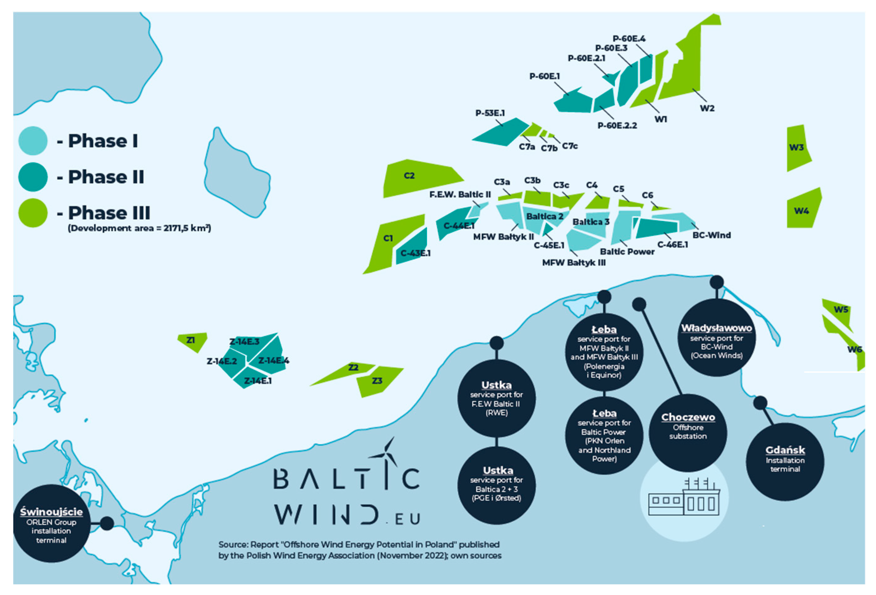
Figure 2.
The arrangement of transported stack of components for 6 turbines on the deck of the installation vessel.
Figure 2.
The arrangement of transported stack of components for 6 turbines on the deck of the installation vessel.
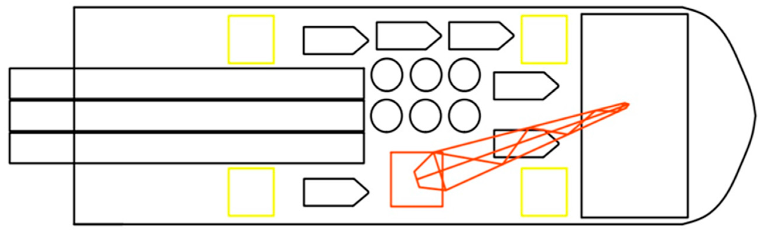
Figure 3.
The relation T = f(B) used to determine the draft of the vessel.
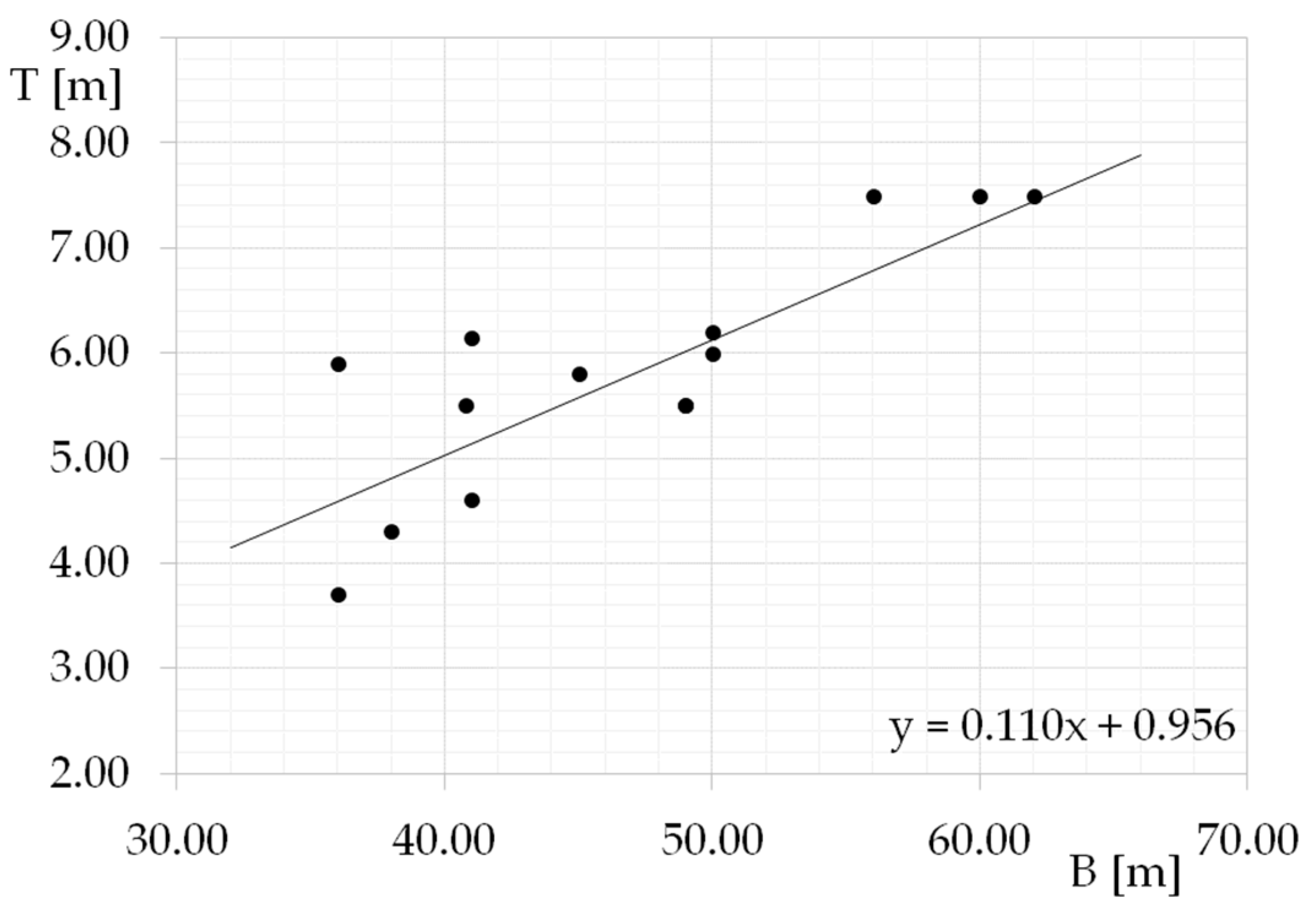
Figure 4.
The relation H = f(T) used to determine the height of the vessel.
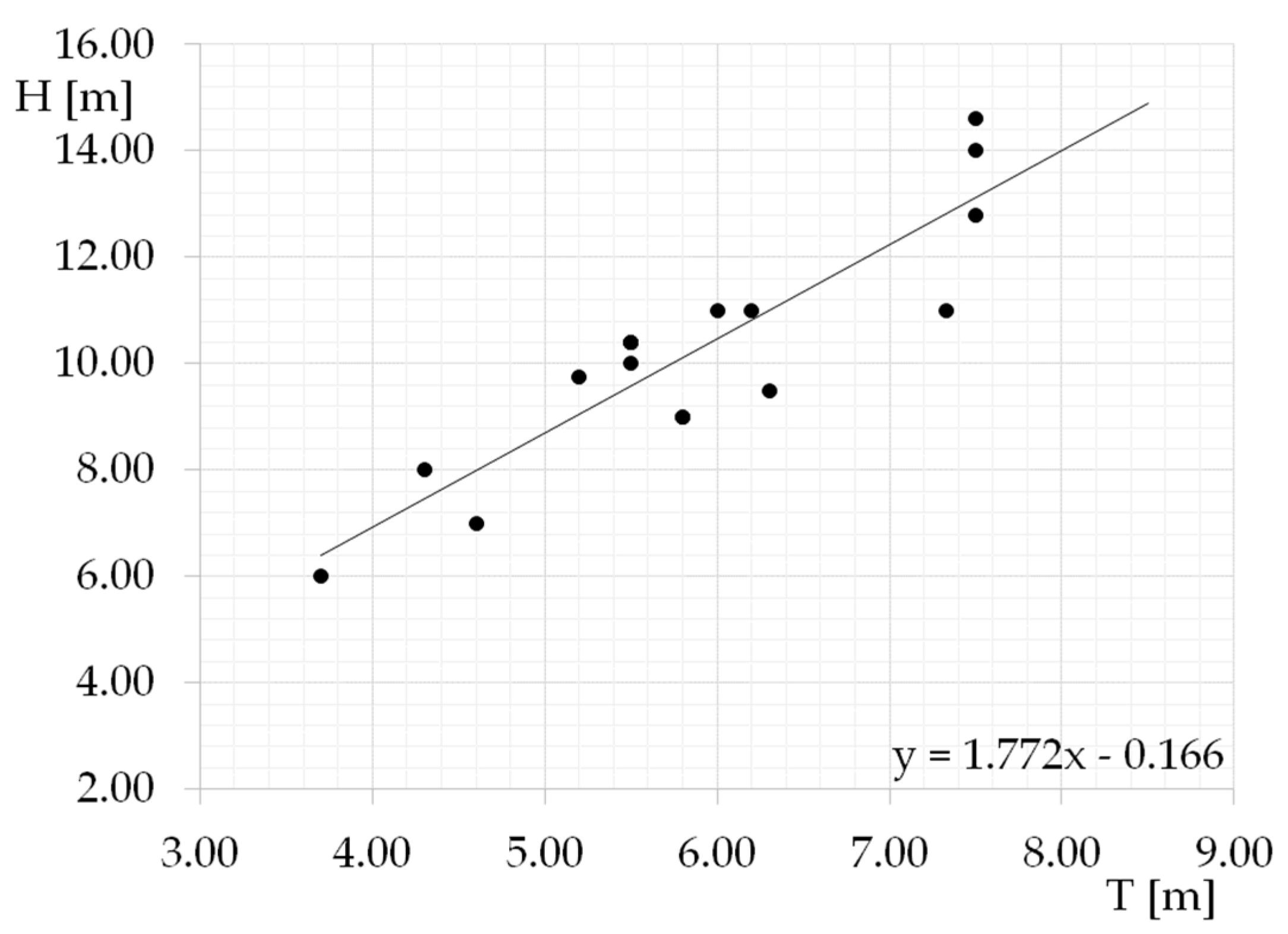
Figure 5.
The relation D = f(LBT) used to determine the displacement of the vessel.
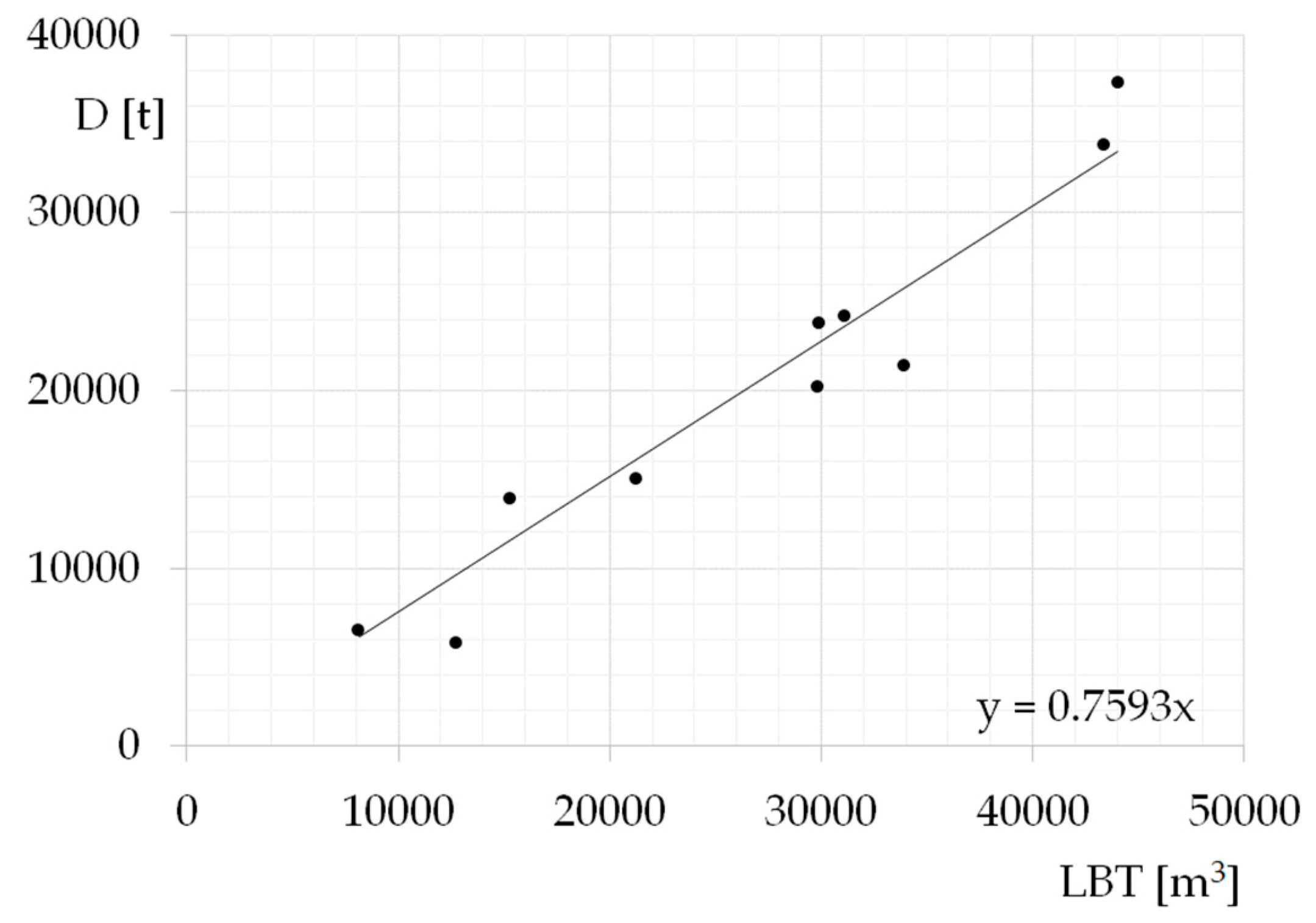
Figure 6.
The lines plan of the design vessel.
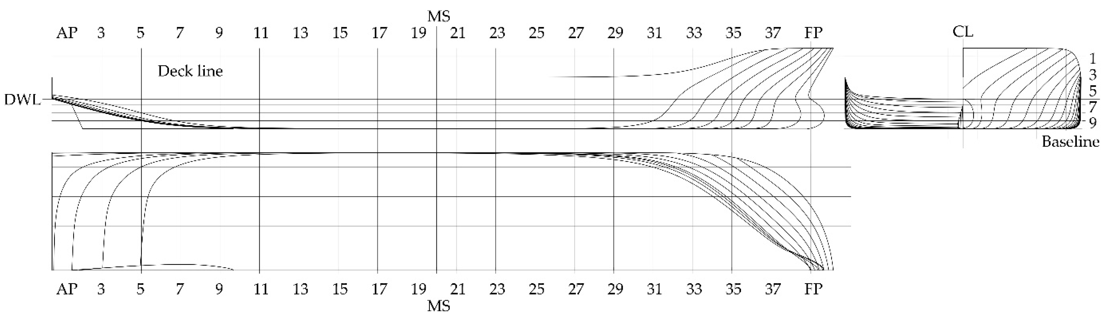
Figure 7.
3D view of the vessel.
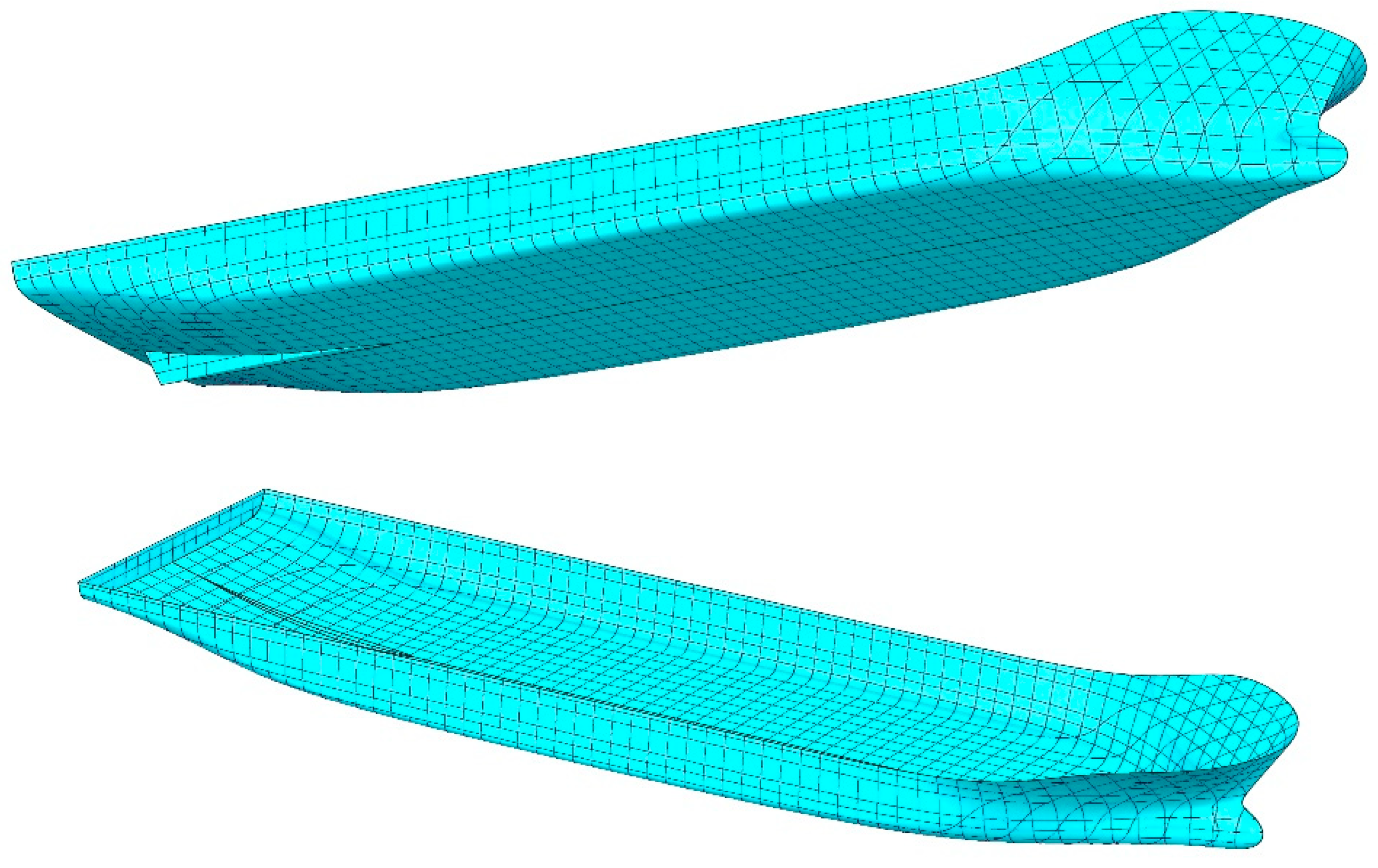
Figure 8.
General arrangement of the designed vessel.
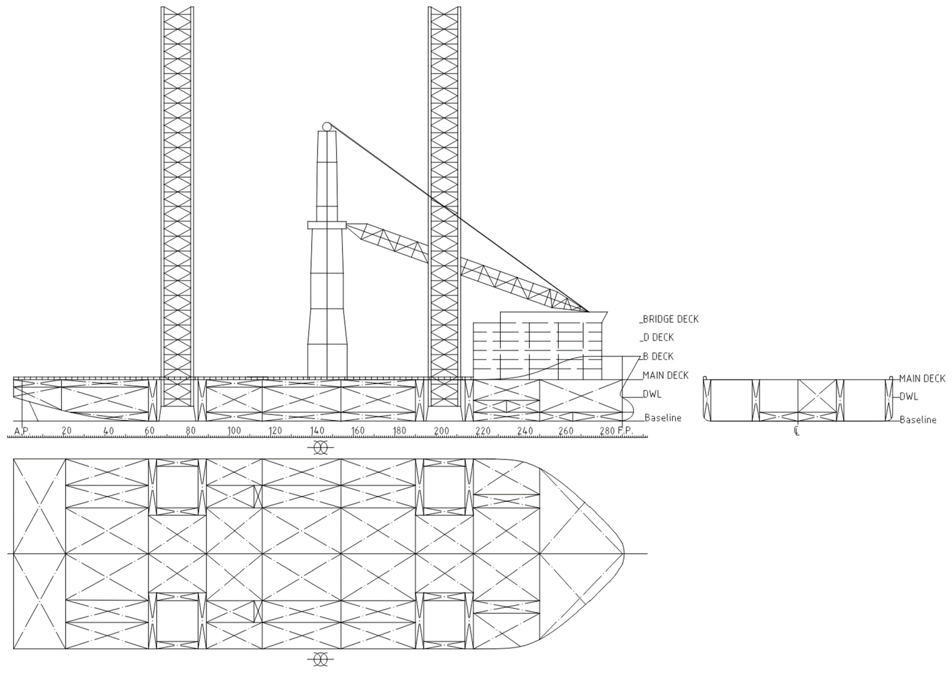
Figure 9.
Contribution of different types of emssion of the wind turbine installation vessel in the total yearly emissions in the shipbuilding, maintenance and dismantling phases.
Figure 9.
Contribution of different types of emssion of the wind turbine installation vessel in the total yearly emissions in the shipbuilding, maintenance and dismantling phases.
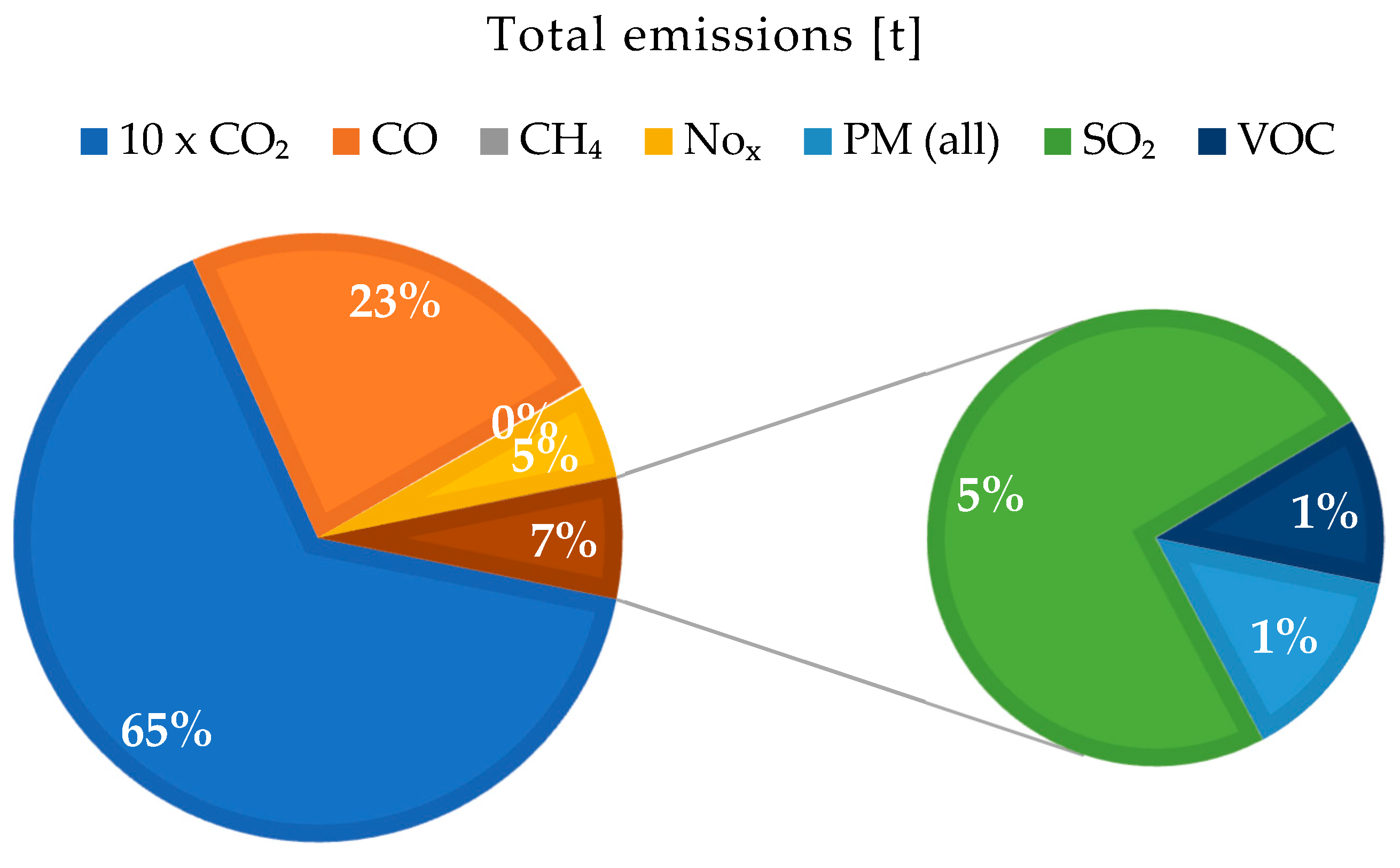
Figure 10.
CO emissions for different phases.
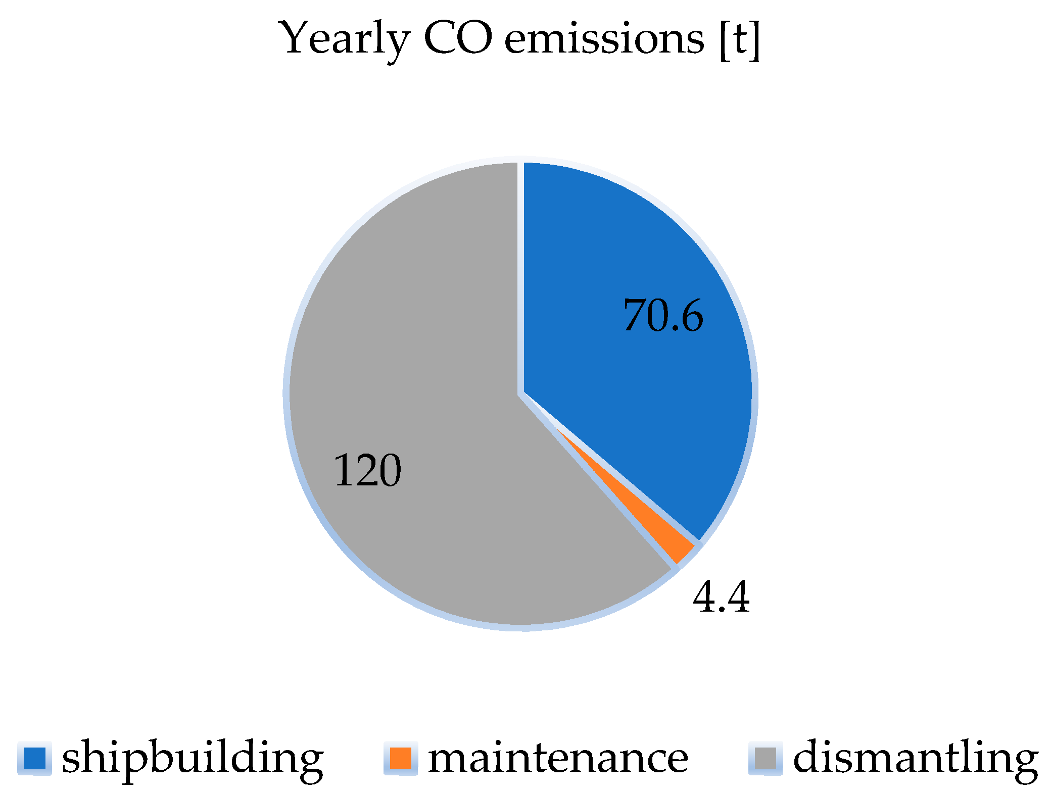
Figure 11.
The comparison of emissions excluding CO2.
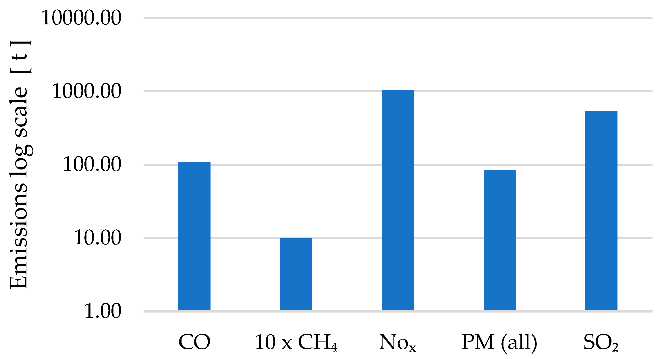

Table 1.
Selected basic design parameters of the similar ships in the list [28,29,30,31,32,33,34,35,36].
| no | Name | Year built | LOA [m] | B/T | L/B | H/T | B [m] | T [m] | H [m] |
|---|---|---|---|---|---|---|---|---|---|
| 1 | Blue Amber | design | 197.00 | 7.47 | 3.52 | 1.87 | 56.00 | 7.50 | 14.00 |
| 2 | Innovation | 2015 | 147.50 | 5.73 | 3.51 | 1.50 | 42.00 | 7.33 | 11.00 |
| 4 | Pacific Orca | 2012 | 160.90 | 8.91 | 3.28 | 1.89 | 49.00 | 5.50 | 10.40 |
| 5 | Seajacks Scylla | 2015 | 139.00 | 8.33 | 2.78 | 1.83 | 50.00 | 6.00 | 11.00 |
| 6 | Ulam | design | 199.09 | 8.27 | 3.21 | 1.71 | 62.00 | 7.50 | 12.80 |
| 7 | Voltaire | 2022 | 169.30 | 8.00 | 2.82 | 1.95 | 60.00 | 7.50 | 14.60 |
| 8 | Vole au vent | 2013 | 140.40 | 6.51 | 3.42 | 1.51 | 41.00 | 6.30 | 9.50 |
Table 2.
Technical parameters of large wind turbines, to be erected by the installation vessel [37].
Table 2.
Technical parameters of large wind turbines, to be erected by the installation vessel [37].
| Part | Height [m] | Weight [t] | Diameter [m] | Length [m] |
|---|---|---|---|---|
| Technical parameters of 10 MW wind turbine | ||||
| Tower | 119 | 605 | 8 | - |
| Nacelle | - | 674 | - | - |
| Blade | - | 41 | - | 86 |
| Technical parameters of 15 MW wind turbine | ||||
| Tower | 150 | 860 | 10 | - |
| Nacelle | - | 1017 | - | - |
| Blade | - | 65 | - | 117 |
Table 3.
Estimated technical parameters of 14 MW wind turbine, to be erected by the designed installation vessel.
Table 3.
Estimated technical parameters of 14 MW wind turbine, to be erected by the designed installation vessel.
| Technical parameters of 14 MW wind turbine | ||||
|---|---|---|---|---|
| Part | Height [m] | Weight [t] | Diameter [m] | Length [m] |
| Tower | 144 | 809 | 9.5 | - |
| Nacelle | - | 948 | - | - |
| Blade | - | 60 | - | 111 |
Table 4.
The summary of estimations of main particulars and mass characteristics.
| Technical characteristics | Symbol | Value | Unit |
|---|---|---|---|
| Length overall | LOA | 212.00 | [m] |
| Waterline length | LWL | 205.80 | [m] |
| Breadth | B | 64.00 | [m] |
| Height | H | 14.00 | [m] |
| Draft | T | 8.00 | [m] |
| Block coefficient | CB | 0.80 | [-] |
| Displacement | D | 86240 | [t] |
| Lightship weight | LSW | 59104 | [t] |
| DWT | DWT | 27136 | [t] |
| Longitudinal center of gravity | LCG | 100,21 | [m] |
| Vertical center of gravity | VCG | 18,07 | [m] |
Table 5.
The summary of estimations of main particulars and mass characteristics.
| Hydrostatics property | Value | Unit |
|---|---|---|
| WL Length | 205.50 | m |
| Breadth max on WL | 63.97 | m |
| Wetted Area | 14230.48 | m2 |
| Max sectional area | 507.29 | m2 |
| Waterplane Area | 11625.19 | m2 |
| Prismatic coefficient (CP) | 0.797 | |
| Block coefficient (CB) | 0.80 | |
| Sectional area coefficient (CM) | 0.99 | |
| Waterplane area coefficient (CWP) | 0.88 | |
| Longitudinal position of buoyancy center KB | 99.68 | from AP [m] |
| Longitudinal position of floatation center LCF | 92.38 | from AP [m] |
| Vertical position of buoyancy center KB | 4.21 | m |
| Bmtrans. | 43.56 | m |
| BMlong. | 405.08 | m |
| Kmtrans. | 47.77 | m |
| KMlong. | 409.29 | m |
| Immersion (TPc) | 119.16 | tonne/cm |
| MTc | 1628.51 | tonne·m |
| hull shape slenderness ratio | 4.72 |
Table 6.
The input data set used for external forces calculation.
| Variable | Symbol | Value | Unit |
|---|---|---|---|
| Wind speed | VA | 10 | [m/s] |
| Current speed | VC | 1 | [m/s] |
| Wave height | HS | 4 | [m] |
| Average wave period | T1 | 5 | [s] |
| Wind direction relative to the vessel | βA | 0÷180 | [o] |
| Wave direction relative to the vessel | βW | 0÷180 | [o] |
| Current direction relative to the vessel | βC | 0÷180 | [o] |
| Coefficients increasing drag relative to environmental forces | CTX, CTY, CTM | 1,1 | [-] |
| Regular wave frequency | ω | 0.2÷0.4 | [1/s] |
Table 7.
Summary of ship’s projected areas.
| Ship particular | Symbol | Value | Unit |
| Projection of the frontal area | SX | 2496 | [m2] |
| Projection of the side area | SY | 4500 | [m2] |
| Projection of the side underwater area in the symmetry plane | F | 1615 | [m2] |
Table 8.
Average wind forces calculation result.
| βA [⁰] | RAX [kN] | RAY [kN] | MAZ [kNm] |
| 0.00 | 60.28 | 0.00 | 0.00 |
| 30.00 | 87.55 | 129.38 | -5145.24 |
| 60.00 | 57.41 | 183.71 | -4720.89 |
| 90.00 | -14.35 | 214.76 | -954.79 |
| 120.00 | -34.44 | 219.94 | 2121.75 |
| 150.00 | -80.37 | 103.50 | 3023.49 |
| 180.00 | -63.15 | 0.00 | 0.00 |
Table 9.
Forces exerted by the current.
| βC [⁰] | RCX [kN] | RCY [kN] | Mcz [kNm] |
| 0 | 8.95 | 0.00 | 0.00 |
| 30 | 20.35 | 325.58 | -11680.33 |
| 60 | 18.72 | 651.17 | -13348.94 |
| 90 | 0.81 | 691.87 | 0.00 |
| 120 | -16.28 | 651.17 | 10011.71 |
| 150 | -22.79 | 325.58 | 11680.33 |
| 180 | -12.21 | 0.00 | 0.00 |
Table 10.
Results of calculations of spectral energy density.
| ω | Value | Unit |
| 0.2 | 1.1E-296 | [m2s] |
| 0.4 | 7.6E-17 | [m2s] |
| 0.6 | 1.1E-02 | [m2s] |
| 0.8 | 9.1E-01 | [m2s] |
| 1.0 | 1.5E+00 | [m2s] |
| 1.2 | 1.0E+00 | [m2s] |
| 1.4 | 6.2E-01 | [m2s] |
Table 11.
Results of wave forces calculations.
| βC [⁰] | Rwx [kN] | Rwy [kN] | Mwz [kNm] |
| 0 | 184.023 | 0.000 | 0.000 |
| 30 | 240.831 | 229.653 | -5748.403 |
| 60 | 301.019 | 897.712 | -4785.262 |
| 90 | -4.339 | 1943.161 | 2005.813 |
| 120 | -344.945 | 951.925 | -8498.818 |
| 150 | -223.605 | 231.779 | 2585.017 |
| 180 | -180.768 | 0.000 | 890.645 |
Table 12.
Results of thrust forces calculation.
| TCX [kN] | TCY [kN] | MCZ [kNm] |
|---|---|---|
| 278.58 | 0.00 | 0.00 |
| 383.60 | 753.07 | -24831.37 |
| 414.86 | 1905.85 | -25140.61 |
| -19.66 | 3134.77 | 1156.13 |
| -435.24 | 2005.33 | 3998.10 |
| -359.44 | 726.95 | 19017.72 |
| -281.74 | 0.00 | 979.71 |
Table 13.
Power loads for stationary installation mode.
| No. | System | Power load max. [kW] |
|---|---|---|
| 1 | Jack up system | 4000 |
| 2 | Main crane | 1500 |
| 4 | Pumps, power plant systems | 500 |
| 5 | Other ship system (HVAC, navigation, lights etc.) | 1200 |
| Total | 6750 |
Table 14.
Power balance for the considered cases.
| Operational mode | Propulsion thrusters [kW] | DP thrusters [kW] | Jack up [kW] | Main crane [kW] | Pumps, power plant, Other loads [kW] | Max. Total load [kW] |
|---|---|---|---|---|---|---|
| Free running transit | 8800 | - | - | - | 1700 | 10500 |
| DP work | 8800 | 10800 | - | - | 1700 | 21300 |
| Jacking up and installation work | - | - | 4000 | 1500 | 1700 | 7200 |
Table 15.
The source data emissions for the reference vessel [2], recalculated for 1 year of operation.
Table 15.
The source data emissions for the reference vessel [2], recalculated for 1 year of operation.
| Emissions 1 year | Operation | Shipbuilding | Maintenance | Dismantling | Total Life Cycle | |
|---|---|---|---|---|---|---|
| CO2 | tons | 42400.00 | 916.00 | 384.80 | 340.40 | 44041 |
| CO | tons | 126.80 | 18.12 | 3.26 | 30.88 | 179 |
| CH4 | tons | 1.12 | 0.16 | 0.06 | 0.09 | 1 |
| NOx | tons | 1216.00 | 5.12 | 3.68 | 4.28 | 1229 |
| PM (all) | tons | 98.00 | 0.92 | 0.35 | 0.90 | 100 |
| SO2 | tons | 628.00 | 4.08 | 2.96 | 5.12 | 640 |
| VOC | tons | 0.80 | 2.31 | 0.01 | 3 |
Table 16.
The specific emission indexes ki.
| Operation | Shipbuilding | Maintenance | Dismantling | |
|---|---|---|---|---|
| Emission | [te*/kW] | [te*/t] | [te*/m2] | [te*/t] |
| CO2 | 4.46E+00 | 6.04E-02 | 3.66E-02 | 2.24E-02 |
| CO | 1.33E-02 | 1.19E-03 | 3.11E-04 | 2.04E-03 |
| CH4 | 1.18E-04 | 1.07E-05 | 5.63E-06 | 5.62E-06 |
| NOx | 1.28E-01 | 3.38E-04 | 3.50E-04 | 2.82E-04 |
| PM (all) | 1.03E-02 | 6.04E-05 | 3.31E-05 | 5.93E-05 |
| SO2 | 6.61E-02 | 2.69E-04 | 2.81E-04 | 3.38E-04 |
| VOC | 5.27E-05 | 2.20E-04 | 7.89E-07 |
te* - tons of emission.
Table 17.
The results of calculation of emissions for shipbuilding, maintenance and dismantling phases.
Table 17.
The results of calculation of emissions for shipbuilding, maintenance and dismantling phases.
| Shipbuilding | Maintenance | Dismantling | Total emissions | |
|---|---|---|---|---|
| emissions yearly | [t] | [t] | [t] | [t] |
| CO2 | 3569.31 | 521.03 | 1326.41 | 5416.75 |
| CO | 70.61 | 4.42 | 120.33 | 195.35 |
| CH4 | 0.63 | 0.08 | 0.33 | 1.04 |
| NOx | 19.95 | 4.98 | 16.68 | 41.61 |
| PM (all) | 3.57 | 0.47 | 3.51 | 7.55 |
| SO2 | 15.90 | 4.00 | 19.95 | 39.85 |
| VOC | 3.12 | 3.13 | 0.05 | 6.29 |
Table 18.
Operational phase emissions calculated for the wind turbine installation vessel – different operational profiles and total emission, yearly.
Table 18.
Operational phase emissions calculated for the wind turbine installation vessel – different operational profiles and total emission, yearly.
| tFR = 6%, | tDP = 23%., kel = 0.6 | tIW = 71 | 100% of op. time | |
| Types of emission | Free Running - Transit | DP operation | Installation Work | Total Emissions |
| [t] | [t] | [t] | [t] | |
| CO2 | 2811.79 | 10932.51 | 22815.66 | 36560 |
| CO | 8.41 | 32.69 | 68.23 | 109 |
| CH4 | 0.07 | 0.29 | 0.60 | 1 |
| NOx | 80.64 | 313.54 | 654.34 | 1049 |
| PM (all) | 6.50 | 25.27 | 52.73 | 85 |
| SO2 | 41.65 | 161.92 | 337.93 | 542 |
Disclaimer/Publisher’s Note: The statements, opinions and data contained in all publications are solely those of the individual author(s) and contributor(s) and not of MDPI and/or the editor(s). MDPI and/or the editor(s) disclaim responsibility for any injury to people or property resulting from any ideas, methods, instructions or products referred to in the content. |
© 2025 by the authors. Licensee MDPI, Basel, Switzerland. This article is an open access article distributed under the terms and conditions of the Creative Commons Attribution (CC BY) license (http://creativecommons.org/licenses/by/4.0/).
Copyright: This open access article is published under a Creative Commons CC BY 4.0 license, which permit the free download, distribution, and reuse, provided that the author and preprint are cited in any reuse.


