On a Higgs-Mediated Relation Between Elementary Particles and Spacetime and Its Physical Consequences

1. Introduction

The Higgs mechanism [1,2] is one of the essential ingredients of the Standard Model (SM), which in turn constitutes the current overall framework for the theoretical study of elementary particles. Initially proposed as a hypothesis aimed at the “soft” introduction (i.e. without loss of renormalizability) of the mass terms into the SM Lagrangian, it has been placed on a secure basis by subsequent experimental results, culminating in the confirmation of the existence of the Higgs boson H₀ in the past decade [3]. Here we propose a theoretical description that traces the Higgs mechanism back to a particular internal geometry of the point-events of physical spacetime, giving it a fundamental value. We show that it is possible to deduce, from this interpretation of the mechanism, a set of non-trivial physical results, even apparently far from the starting argument. Some of these results are already known, but are here obtained within the framework of a line of reasoning more stringent than the conventional one, while others are completely new. Among these results we point out: 1) a simple explanation of the spatial delocalization of particles and of their behavior in experiments such as the double slit one; 2) a coherent explanation of quantum jumps; 3) a classicalization mechanism, in principle experimentally testable, independent of the existence of environmental degrees of freedom; 4) a theory of flavor mixing in the weak interaction mediated by charged current, with a calculation scheme of the mixing coefficients; 5) a possible solution to the problem of the discrepancy between vacuum energy and cosmological constant.

The idea behind the proposal is the following. It is assumed that ordinary spacetime is immersed in a five-dimensional Euclidean space E₅ and that each point-event is the point of tangency, on spacetime, of a de Sitter space immersed in E₅. It is assumed that the spaces tangent to the same point-event or to nearby point-events, although they can geometrically penetrate and intersect each other in E₅, are non-interacting, in the sense that the matter distributed in one of these spaces interacts only with the matter present in the same space. In other words, matters belonging to different spaces do not “see” each other; this is equivalent to defining the de Sitter space, tangent to spacetime at a defined point-event, as an internal structure of that point.

Instead, it is assumed that distinct elements of matter belonging to the same space influence each other through the gravitational interaction internal to that space. It should be noted that this interaction is not the gravitational interaction acting on spacetime and well known to us; in particular, the internal gravitational constant of the de Sitter space considered, which regulates the interaction between the elements of matter contained in it, is not Newton's gravitational constant. Matter is assumed to be distributed, within the single de Sitter space, according to a homogeneous and constant density sized both by the vacuum expectation value (VEV) of the Higgs field and by the mass of the Higgs boson [4]. By imposing that the density is a source of negative pressure, the de Sitter space can be obtained as a solution to Einstein's gravitational equations according to an appropriate choice of the internal gravitational constant. This construction then connects the Higgs vacuum to a multiplicity of de Sitter spaces in one-to-one correspondence with the point-events of spacetime through a tangency relation, and it is equivalent to defining an internal geometry of the point-events. It is then possible to consider a further set of de Sitter spaces, tangent to each point-event of spacetime, whose internal gravitational constant is defined in accordance with a total mass content proportional to the VEV with a fixed proportionality constant, as prescribed by the SM for elementary fermions. These spaces are a rescaled version of the spaces associated with the VEV, and are solutions of the same gravitational equations with a different value of the gravitational constant. They can be considered as a version of the de Sitter spaces associated with the VEV but with a different energy content. Each of these spaces then implements a single positional eigenstate of a quantum entity that is an elementary particle (elementary fermion) of the SM [5].

One can select n spaces associated with the positional eigenstates of n distinct particles; the set of spaces thus selected corresponds to the tensorial product of n positional eigenstates of these particles. While this product “lives” on the configurational space of the n particles, the points of tangency of the de Sitter spaces so selected belong to the usual spacetime.

The quantum entity “elementary particle” is, in this line of reasoning, defined as a particular solution of the quantum extension of Einstein’s gravitational equations, i.e. as a solution of a suitably chosen Wheeler-de Witt (WdW) equation. Among the asymptotic solutions of this equation, the harmonic and the decreasing exponential ones are of particular interest. The harmonic solutions depend on a time parameter defined by the distance scale, which can be connected to the internal global time of the de Sitter space. We identify this variable with the particle’s proper time, measured by an external observer “at rest” with respect to it. It can be related to the internal closed slicing time. The application of the relativistic covariance rules transforms the harmonic solution into a de Broglie plane phase wave, delocalized over the entire space of contemporaneity of the particle in spacetime. From the linearity of the evolution equation it follows that the most general free solution is given by the generic superposition of plane waves that satisfies the dispersion relation. We then obtain the Klein-Gordon equation. In summary: the Higgs mechanism defines the mass of the SM particles, and therefore also their proper time, conjugated to the mass. The fact that the evolution of the particles is defined only by the proper time is the origin of the spatial delocalization of these quantum entities [6].

Exponential solutions do not support the relation between internal time of de Sitter space and external time measurable by an observer; they are therefore related to physical situations in which the evolution of the particle in external time stops. Their further characteristics are evanescence and violation of unitarity. These solutions therefore describe instantaneous processes of disappearance of the particle state from spacetime or of appearance of the same state in spacetime, or both. We propose to use them to model the discontinuous variation of the particle state, i.e. quantum jumps, thus providing a dynamical basis for the projection postulate [7,8].

The possibility of describing in dynamical terms the state reduction processes as effects of the ordinary interactions between elementary particles described by SM solves an old conceptual problem of quantum theories [9]. It also allows the construction of classicalization models that are not affected by the traditional problems of the absence of selection and justification of the preferred basis [10]. The decoherence involved in these models implies an actual violation of unitarity at the microscopic level, and not a mere concealment of coherence through the trace operation on the environmental degrees of freedom; the latter, in fact, are not relevant in this description. This element can in principle allow the experimental distinction between the proposed classicalization scheme and others based on a more conventional view of decoherence.

The redefinition of elementary particles as quantum de Sitter spaces tangent to spacetime (with a quantum delocalized tangency point) implies the need to consequently redefine the interaction of SM elementary fermions with gauge bosons (γ, W^±, Z₀, H₀, gluons, graviton). The model we propose assumes that in the free propagation phase the gauge bosons are structureless, while in the coupling with external fermionic lines the single boson dissociates into a pair of elementary fermions; one of these annihilates the entering state, while the other appears as the exiting state. If the fermionic states entering (exiting) the vertex are two, both are annihilated (created) by the pair of elementary fermions generated by the dissociation, thus giving rise to the annihilation (creation) of a pair. The process can be described with diagrams that can be related to Feynman diagrams, although they are distinct from them. The dissociation mechanism is studied in some detail, and it is shown that only in weak interactions mediated by charged current does flavor mixing occur. A calculation of the amplitude of the interaction vertex is proposed and it is shown that it is diagonalized, on the basis of flavors, by the experimental mixing matrices (Cabibbo-Kobayashi-Maskawa or CKM for quarks, Pontecorvo-Maki-Nakagawa-Sakata or PMNS for leptons). A further, more speculative, application of the interaction-induced gauge boson dissociation scheme concerns the photon, and consists in an attempt to derive its coupling constant (fine structure constant).

The finite value of the de Sitter radius of elementary particles implies a finite value of the energy required for an interaction to create a positional eigenstate of a particle. Since, in such creation, the energy involved in the process self-interacts gravitationally, the existence of a lower limit of such self-interaction is demonstrated. This limit defines, in a natural way, the cosmological constant. The latter then comes to represent a structural constraint connected to the potential processes of localization of matter in spacetime, without relation to the vacuum energy. This result constitutes a possible way out of the gigantic discrepancy between vacuum energy and the cosmological constant.

The scheme proposed for the elementary fermions of the SM could be extended also to hadrons, by replacing the vacuum expectation value of the Higgs field with that of the mesonic fields of phenomenological models with spontaneous symmetry breaking, such as the sigma model [11,12]. The single hadron then corresponds to a de Sitter space tangent to spacetime [13,14,15]. The points of tangency of the de Sitter spaces of the quarks belonging to the hadron are confined within the vertical projection of the hadronic de Sitter space on spacetime. This confinement is obtained automatically if one assumes that the strong charge of quarks and gluons is in fact dislocated on the hadronic de Sitter space, and only projected on spacetime [16,17,18]. One thus obtains a simple ab initio explanation of the confinement, both geometric and color.

The plan of the presentation is as follows. The basic principles and assumptions are stated in Section 2. Subsections 2.1, 2.2 present the geometric representation of the Higgs vacuum and of the elementary fermions of the SM, in essentially semiclassical terms. The transition to quantization, via the WdW equation, is described in subsection 2.3. A suitable physical interpretation of the harmonic solutions of the WdW allows the introduction of elementary particles as spatially delocalized entities described by quantum-relativistic wave equations, an aspect that is discussed in subsection 2.4. The exponential solutions of the WdW are interpreted as a formal description of quantum jumps in subsection 2.5.

In subsection 2.6 this dynamic description of the quantum discontinuity, which completes the usual Von Neumann projection postulate, is applied to the problem of decoherence and classicalization, with the discussion of specific examples. Subsection 2.7 is devoted to an interpretation of the cosmological constant in the terms already exposed, with some numerical evaluations. Subsection 2.8 is a marginal note referring to previous works and discusses the possible extension of the line of reasoning of the paper to the hadronic case. In particular, the possibility of defining, within the proposed scheme, an ab initio confinement condition both in geometric and color terms is recalled.

Section 3 is devoted to the SM gauge bosons. Subsection 3.1 qualitatively presents a model of the interaction between these bosons and the SM elementary fermions within the conceptual framework outlined above. The model is detailed in subsection 3.2. Subsection 3.3 presents the proposed interaction mechanism in graphical form, and contains only diagrams. These are compared to traditional Feynman diagrams in order to facilitate a visualization of the processes described in the previous subsection. Subsection 3.4 is an attempt to justify the value of the fine structure constant on the basis of the model detailed in subsection 3.2. Subsection 3.5 is devoted to the computation of the mixing parameters of the charged current-mediated weak interaction. Conclusions are given in Section 4.

2. Basic Principles

2.1. A Representation of the Higgs Vacuum

Let us consider Einstein's gravitational equations with cosmological term:

$$R_{\mu \nu }\hspace{0.17em}\hspace{0.17em}-\hspace{0.17em}\hspace{0.17em}\hspace{0.17em}{\displaystyle \frac{R}{2}}\hspace{0.17em}{g}_{\mu \nu }\hspace{0.17em}\hspace{0.17em}+\hspace{0.17em}\hspace{0.17em}\hspace{0.17em}\hspace{0.17em}{\Lambda }_0{g}_{\mu \nu }\hspace{0.17em}\hspace{0.17em}=\hspace{0.17em}\hspace{0.17em}\chi T_{\mu \nu }$$

(1)

with the usual meaning of the terms. Let us consider the case in which matter can be schematized as an ideal fluid with mass density η, which we will assume to be homogeneous and constant, and four-velocity u_μ:

$$T_{\mu \nu }\hspace{0.17em}\hspace{0.17em}=\hspace{0.17em}\hspace{0.17em}\left(\eta \hspace{0.17em}\hspace{0.17em}+\hspace{0.17em}\hspace{0.17em}{\displaystyle \frac{p}{c^2}}\right)\hspace{0.17em}{u}_{\mu }{u}_{\nu }\hspace{0.17em}\hspace{0.17em}+\hspace{0.17em}\hspace{0.17em}p{g}_{\mu \nu }$$

(2)

For a negative pressure p with p + ηc² = 0, Eq.(1) becomes:

$$R_{\mu \nu }\hspace{0.17em}\hspace{0.17em}-\hspace{0.17em}\hspace{0.17em}\hspace{0.17em}{\displaystyle \frac{R}{2}}\hspace{0.17em}{g}_{\mu \nu }\hspace{0.17em}\hspace{0.17em}+\hspace{0.17em}\hspace{0.17em}\hspace{0.17em}\hspace{0.17em}({\Lambda }_0\hspace{0.17em}+\hspace{0.17em}\chi \eta c^2)g_{\mu \nu }\hspace{0.17em}\hspace{0.17em}=\hspace{0.17em}\hspace{0.17em}\hspace{0.17em}\hspace{0.17em}0$$

(3)

which is the equation of a de Sitter space with an "effective" cosmological constant Λ = Λ₀ + χηc². If Λ₀ = 0, we have Λ = χηc² = R. We note that it is possible to arrive at the same result if we start from the full contraction of Eq.(1) without a cosmological term:

$$2R\hspace{0.17em}\hspace{0.17em}=\hspace{0.17em}\hspace{0.17em}{\displaystyle \frac{8\pi G}{c^4}}\hspace{0.17em}T\hspace{0.17em}$$

(4)

(where we placedχ = 8πG/c⁴), noting that for a negative pressure p = -ηc²we have:

$$T_{\mu \nu }\hspace{0.17em}\hspace{0.17em}=\hspace{0.17em}\hspace{0.17em}\left(\eta \hspace{0.17em}+\hspace{0.17em}{\displaystyle \frac{p}{c^2}}\right)u_{\mu }{u}_{\nu }\hspace{0.17em}\hspace{0.17em}+p{g}_{\mu \nu }\hspace{0.17em}\hspace{0.17em}\hspace{0.17em}=\hspace{0.17em}\hspace{0.17em}\hspace{0.17em}p{g}_{\mu \nu }\hspace{0.17em}\hspace{0.17em}\hspace{0.17em}\hspace{0.17em}\Rightarrow \hspace{0.17em}\hspace{0.17em}\hspace{0.17em}\hspace{0.17em}T\hspace{0.17em}\hspace{0.17em}=\hspace{0.17em}\hspace{0.17em}{g}^{\mu \nu }{T}_{\mu \nu }\hspace{0.17em}\hspace{0.17em}=\hspace{0.17em}\hspace{0.17em}-2p\hspace{0.17em}\hspace{0.17em}=\hspace{0.17em}\hspace{0.17em}2\eta c^2$$

(5)

and therefore:

$$R\hspace{0.17em}\hspace{0.17em}=\hspace{0.17em}\hspace{0.17em}{\displaystyle \frac{8\pi G}{c^4}}\hspace{0.17em}\eta c^2\hspace{0.17em}\hspace{0.17em}=\hspace{0.17em}\hspace{0.17em}\hspace{0.17em}{\displaystyle \frac{3}{r_{dS}^2}}$$

(6)

where r_dS is the de Sitter radius of the space described by Eq.(6).

Let us now consider the Higgs field, which is introduced in the usual way, as an iso-doublet Ω of scalar fields defined on the space SU(2) of the weak isospin. These fields will depend on the spacetime position. We denote by ε (having the dimensions of an energy) the expectation value of the vacuum (VEV), defined in the usual way. Let’s consider the energy e defined by the relation:

$${\left|\hspace{0.17em}\Omega \hspace{0.17em}\right|}^2\hspace{0.17em}\hspace{0.17em}\hspace{0.17em}=\hspace{0.17em}\hspace{0.17em}\hspace{0.17em}\hspace{0.17em}{\Omega }^{+}\Omega \hspace{0.17em}\hspace{0.17em}\hspace{0.17em}=\hspace{0.17em}\hspace{0.17em}\hspace{0.17em}\hspace{0.17em}\epsilon \hspace{0.17em}e$$

(7)

The symmetry breaking, that is the passage from e = 0 (the "false vacuum") to e = ε (the "true vacuum"), corresponds in the SU(2) space to the choice of a specific direction of the spinor Ω of norm ε as the new vacuum state. |Ω| = ε must be a stable point of the potential of the free Higgs field. Therefore, this potential must be even in ε(e - ε) and then be expressed by a sum of even powers of (|Ω|² - ε²). The only possibility compatible with renormalization is that of a completely harmonic dynamics of the variable ε(e - ε), in accordance with the usual choice of a potential proportional to ε²(e - ε)², that is (|Ω|² - ε²)².

Having made these premises, let us now come to the idea underlying our proposal. It consists in assuming that spacetime is immersed in an E₅ space, and that each point-event of spacetime is the point of tangency, on spacetime, of a de Sitter space in E₅. We assume that these spaces are non-interacting in the sense that, although spaces tangent to the same point-event or to nearby point-events can overlap or intersect in E₅, the matter contained in the regions of overlap interacts only with the matter located in the same space. In other words, the matter of each space does not “see” the matter of other spaces. As regards the interaction of distinct portions of matter of the same space, we assume that it is of a single type, that is, that it is a gravitational interaction describable through Eq.(1). A crucial observation at this point is the following: there is no reason why the gravitational constant G internal to these spaces should coincide with Newton's gravitational constant operating on spacetime. In fact, these are entirely different spaces between which there exists a mere geometric relation of tangency. There is no relationship between the internal gravitation of these spaces and the "external" gravitation acting on spacetime. It is then possible to consider the situation in which the tangent spaces are solutions of Eq.(6) with the conditions:

$$G\hspace{0.17em}\hspace{0.17em}\hspace{0.17em}=\hspace{0.17em}\hspace{0.17em}\hspace{0.17em}{\displaystyle \frac{\hslash c}{{\left(\frac{\epsilon }{c^2}\right)}^2}}\hspace{0.17em}\hspace{0.17em}=\hspace{0.17em}\hspace{0.17em}{G}_0\hspace{0.17em}$$

(8)

and:

$$r_{dS}\hspace{0.17em}\hspace{0.17em}\hspace{0.17em}=\hspace{0.17em}\hspace{0.17em}\hspace{0.17em}{\displaystyle \frac{\hslash }{M_{H_0}c}}\hspace{0.17em}\hspace{0.17em}=\hspace{0.17em}\hspace{0.17em}{r}_{dS,0}$$

(9)

where M_H0 is the mass of the Higgs boson H₀. As can be seen from Eq.(6), the solution exists if:

$$\eta \hspace{0.17em}\hspace{0.17em}\hspace{0.17em}=\hspace{0.17em}\hspace{0.17em}\hspace{0.17em}{\eta }_0\hspace{0.17em}\hspace{0.17em}\hspace{0.17em}=\hspace{0.17em}\hspace{0.17em}\hspace{0.17em}{\displaystyle \frac{M_{H_0}^2{c}^4}{{\hslash }^2}}\hspace{0.17em}\hspace{0.17em}\hspace{0.17em}{\left({\displaystyle \frac{\epsilon }{c^2}}\right)}^2\hspace{0.17em}\hspace{0.17em}{\displaystyle \frac{3}{8\pi \hslash c}}\hspace{0.17em}\hspace{0.17em}$$

(10)

that is, if the density is chosen as a suitable function of the constants M_H0 and ε. Denoting with M the total mass content of space:

$$\eta \hspace{0.17em}\hspace{0.17em}\hspace{0.17em}=\hspace{0.17em}\hspace{0.17em}\hspace{0.17em}{\displaystyle \frac{M}{\frac{8\pi }{3}\hspace{0.17em}{\left(\frac{k\hslash }{Mc}\right)}^3}}\hspace{0.17em}\hspace{0.17em}\hspace{0.17em}=\hspace{0.17em}\hspace{0.17em}\hspace{0.17em}{\displaystyle \frac{3}{8\pi }}\hspace{0.17em}{\displaystyle \frac{M^4{c}^3}{{\hslash }^3{k}^3}}\hspace{0.17em}\hspace{0.17em}$$

(11)

where:

$$r_{dS}\hspace{0.17em}\hspace{0.17em}=\hspace{0.17em}\hspace{0.17em}{\displaystyle \frac{k\hslash }{Mc}}\hspace{0.17em}$$

(12)

then η₀ turns out to be the geometric mean of the following densities computed with k = 1:

$${\eta }_{H_0}\hspace{0.17em}\hspace{0.17em}\hspace{0.17em}=\hspace{0.17em}\hspace{0.17em}\hspace{0.17em}{\displaystyle \frac{3}{8\pi }}\hspace{0.17em}{\displaystyle \frac{M_{H_0}^4{c}^3}{{\hslash }^3}}\hspace{0.17em}\hspace{0.17em}\hspace{0.17em}$$

(13)

$${\eta }_{\epsilon }\hspace{0.17em}\hspace{0.17em}\hspace{0.17em}=\hspace{0.17em}\hspace{0.17em}\hspace{0.17em}{\displaystyle \frac{3}{8\pi }}\hspace{0.17em}{\displaystyle \frac{{\left(\frac{\epsilon }{c^2}\right)}^4{c}^3}{{\hslash }^3}}\hspace{0.17em}\hspace{0.17em}\hspace{0.17em}$$

(14)

that is:

$${\eta }_0\hspace{0.17em}\hspace{0.17em}=\hspace{0.17em}\hspace{0.17em}\sqrt{\hspace{0.17em}{\eta }_{H_0}\hspace{0.17em}{\eta }_{\epsilon }\hspace{0.17em}\hspace{0.17em}}$$

(15)

The mass content of space is then:

$${\displaystyle \frac{8\pi }{3}}\hspace{0.17em}{\eta }_0\hspace{0.17em}{\left({\displaystyle \frac{\hslash }{M_{H_0}c\hspace{0.17em}}}\right)}^3\hspace{0.17em}\hspace{0.17em}\hspace{0.17em}\hspace{0.17em}=\hspace{0.17em}\hspace{0.17em}\hspace{0.17em}\hspace{0.17em}\hspace{0.17em}{M}_{H_0}^{-1}\hspace{0.17em}{\left({\displaystyle \frac{\epsilon }{c^2}}\right)}^2\hspace{0.17em}$$

(16)

as one might expect from (15). The physical idea is that the VEV of the Higgs field is nothing more than a measure of the gravitational constant (8), while the mass of the Higgs boson is a measure of the de Sitter radius (9) or the curvature –R₀ = 3/r_dS,0². Another way to define the same physical situation [4] is to write the self-interaction potential of the field in the form:

$$V(\Omega )\hspace{0.17em}\hspace{0.17em}\hspace{0.17em}=\hspace{0.17em}\hspace{0.17em}\hspace{0.17em}{\displaystyle \frac{\sqrt{Det(g_{\mu \nu })}}{4\pi }}\hspace{0.17em}\hspace{0.17em}\left[{\displaystyle \frac{R_0}{6}}\hspace{0.17em}{\Omega }^{+}\Omega \hspace{0.17em}\hspace{0.17em}-\hspace{0.17em}\hspace{0.17em}{\displaystyle \frac{{\chi }_0{R}_0}{36}}\hspace{0.17em}{\left({\Omega }^{+}\Omega \right)}^2\right]\hspace{0.17em}$$

(17)

whereχ₀ = 8πG₀/c⁴. Posing:

$$R_0\hspace{0.17em}\hspace{0.17em}\hspace{0.17em}=\hspace{0.17em}\hspace{0.17em}\hspace{0.17em}6{\mu }^2\hspace{0.17em}\hspace{0.17em}\hspace{0.17em}\hspace{0.17em}\hspace{0.17em}\hspace{0.17em}\hspace{0.17em}\hspace{0.17em}\hspace{0.17em}\hspace{0.17em}$$

(18)

and assuming the conventional relation between the VEV and the mass M_W of the W boson:

$$\epsilon \hspace{0.17em}\hspace{0.17em}\hspace{0.17em}\hspace{0.17em}=\hspace{0.17em}\hspace{0.17em}\hspace{0.17em}\hspace{0.17em}\hspace{0.17em}{\displaystyle \frac{\sqrt{2}\hspace{0.17em}{c}^2}{g}}\hspace{0.17em}{M}_W\hspace{0.17em}\hspace{0.17em}$$

(19)

(g represents the electroweak coupling constant), from the expansion around ε in the usual way we then have:

$$\epsilon \hspace{0.17em}\hspace{0.17em}\hspace{0.17em}\hspace{0.17em}\hspace{0.17em}=\hspace{0.17em}\hspace{0.17em}\hspace{0.17em}\hspace{0.17em}{c}^2\hspace{0.17em}{\left({\displaystyle \frac{3}{{\chi }_0}}\right)}^{1/2}\hspace{0.17em}\hspace{0.17em}\hspace{0.17em}\hspace{0.17em}\hspace{0.17em}\Rightarrow \hspace{0.17em}\hspace{0.17em}\hspace{0.17em}\hspace{0.17em}\hspace{0.17em}\hspace{0.17em}\hspace{0.17em}\hspace{0.17em}\hspace{0.17em}{\chi }_0\hspace{0.17em}\hspace{0.17em}=\hspace{0.17em}\hspace{0.17em}{\displaystyle \frac{3}{2}}\hspace{0.17em}{\displaystyle \frac{g^2}{M_W^2}}\hspace{0.17em}\hspace{0.17em}$$

(20)

$$M_{H_0}\hspace{0.17em}\hspace{0.17em}\hspace{0.17em}=\hspace{0.17em}\hspace{0.17em}\hspace{0.17em}{\displaystyle \frac{\hslash }{c}}\hspace{0.17em}{\left(-\hspace{0.17em}{\displaystyle \frac{R_0}{3}}\right)}^{1/2}\hspace{0.17em}\hspace{0.17em}\hspace{0.17em}\hspace{0.17em}\hspace{0.17em}\Rightarrow \hspace{0.17em}\hspace{0.17em}\hspace{0.17em}\hspace{0.17em}\hspace{0.17em}\hspace{0.17em}\hspace{0.17em}{R}_0\hspace{0.17em}\hspace{0.17em}=\hspace{0.17em}\hspace{0.17em}-\hspace{0.17em}{\displaystyle \frac{3M_{H_0}^2{c}^2}{{\hslash }^2}}\hspace{0.17em}\hspace{0.17em}$$

(21)

$$V(\Omega )\hspace{0.17em}\hspace{0.17em}\hspace{0.17em}=\hspace{0.17em}\hspace{0.17em}\hspace{0.17em}{\mu }^2\hspace{0.17em}{\Omega }^{+}\Omega \hspace{0.17em}\hspace{0.17em}+\hspace{0.17em}\hspace{0.17em}\lambda \hspace{0.17em}{\left({\Omega }^{+}\Omega \right)}^2\hspace{0.17em}\hspace{0.17em}\hspace{0.17em}$$

(22)

where λ = -χ₀R₀/36 and:

$${\mu }^2\hspace{0.17em}\hspace{0.17em}=\hspace{0.17em}\hspace{0.17em}\hspace{0.17em}\hspace{0.17em}-{\displaystyle \frac{1}{2}}\hspace{0.17em}{\displaystyle \frac{M_{H0}^2{c}^2}{{\hslash }^2}}\hspace{0.17em}\hspace{0.17em}$$

(23)

We can now note that in general, substituting (11), (12) in (6) we have:

$$G\hspace{0.17em}\hspace{0.17em}=\hspace{0.17em}\hspace{0.17em}{\displaystyle \frac{k\hslash c}{M^2}}\hspace{0.17em}$$

(24)

This result can be obtained by replacing, in (8), ε/c² with M/k^1/2. This allows us to extend the representation to the elementary fermions of the SM. According to the SM, the mass M of the fermion is proportional to the VEV, the constant of proportionality being the coupling constant of the fermion to the Higgs field. We therefore have (M/k^1/2) = f(ε/c²) and therefore, from (8) and (24), G = G₀/f². In other words, the genesis of the mass M of the fermion (more correctly, of the ratio M/k^1/2; we will see the meaning of the factor k in a subsequent subsection) derives from a rescaling of the internal gravitational constant, which in turn induces a new de Sitter radius expressed no longer by (9), but by (12).

Thus, the positional eigenstate of a SM elementary fermion will in fact be associated not to the point-event O, but to the fermionic de Sitter space tangent to O, solution of (6) with gravitational constant (24), de Sitter radius (12) and density (11). The mass content of this space is:

$${\displaystyle \frac{8\pi }{3}}\hspace{0.17em}\eta \hspace{0.17em}{\left({\displaystyle \frac{\hslash }{Mc\hspace{0.17em}}}\right)}^3\hspace{0.17em}\hspace{0.17em}\hspace{0.17em}\hspace{0.17em}=\hspace{0.17em}\hspace{0.17em}\hspace{0.17em}\hspace{0.17em}\hspace{0.17em}M\hspace{0.17em}$$

(25)

as can be easily verified by direct substitution of (11). For the particles we therefore have the following scaling relations:

$${\displaystyle \frac{r_{dS}^2}{r_0^2}}\hspace{0.17em}\hspace{0.17em}=\hspace{0.17em}\hspace{0.17em}{\displaystyle \frac{M_0^2}{M^2}}\hspace{0.17em}\hspace{0.17em}=\hspace{0.17em}\hspace{0.17em}{\displaystyle \frac{G}{G_0}}\hspace{0.17em}\hspace{0.17em}=\hspace{0.17em}\hspace{0.17em}{\displaystyle \frac{1}{f^2}}\hspace{0.17em}\hspace{0.17em}$$

(26)

where:

$$r_0\hspace{0.17em}\hspace{0.17em}=\hspace{0.17em}\hspace{0.17em}\sqrt{k}\hspace{0.17em}\hspace{0.17em}{\displaystyle \frac{\hslash c}{\epsilon }}\hspace{0.17em};\hspace{0.17em}\hspace{0.17em}\hspace{0.17em}\hspace{0.17em}\hspace{0.17em}\hspace{0.17em}\hspace{0.17em}\hspace{0.17em}\hspace{0.17em}\hspace{0.17em}\hspace{0.17em}\hspace{0.17em}\hspace{0.17em}{M}_0\hspace{0.17em}\hspace{0.17em}=\hspace{0.17em}\hspace{0.17em}\hspace{0.17em}\sqrt{k}\hspace{0.17em}\hspace{0.17em}{\displaystyle \frac{\epsilon }{c^2}}\hspace{0.17em}\hspace{0.17em}$$

(27)

The replacement of the VEV of the Higgs field, ε, with the rest energy of the fermion, Mc² ∝ ε, can be seen as the passage from the Higgs field to a scalar field ξ, internal to the fermionic de Sitter space, whose VEV reproduces ξ₀ = Mc²/k^1/2. We then obtain U(ξ) = [ξ² – (Mc²)²/k]². Therefore, ξ₀/(8πr_dS³/3) = p/k^1/2, where p is the pressure modulus. It is possible to introduce the dimensionless self-potential:

$$V\left(\xi \right)\hspace{0.17em}\hspace{0.17em}=\hspace{0.17em}\hspace{0.17em}{\displaystyle \frac{U\left(\xi \right)}{{\left(M{c}^2\right)}^2}}\hspace{0.17em}\hspace{0.17em}=\hspace{0.17em}\hspace{0.17em}{\left[{\left({\displaystyle \frac{\xi }{M{c}^2}}\right)}^2\hspace{0.17em}\hspace{0.17em}-\hspace{0.17em}\hspace{0.17em}{\left({\displaystyle \frac{1}{k^{1/2}}}\right)}^2\right]}^2\hspace{0.17em}\hspace{0.17em}\hspace{0.17em}=\hspace{0.17em}\hspace{0.17em}\hspace{0.17em}{\left({\xi }^2\hspace{0.17em}\hspace{0.17em}-\hspace{0.17em}\hspace{0.17em}{\xi }_0^2\right)}^2\hspace{0.17em}\hspace{0.17em}$$

(28)

where ξ, ξ₀ are now dimensionless and ξ₀ = 1/k^1/2. For continuity with previous works [16] we will also express, without any loss of generality, the dimensionless quantity ξ as ξ = r/r_dS, where r is a length of positive, zero or negative value.

2.2. Digression on the K Factor

In Eq. (12) we have inserted a factor k that converts the Compton wavelength of the particle into the de Sitter radius of the space associated with it. We now want to clarify the physical meaning of this factor. Consider two interacting elementary fermions, 1 and 2, and let:

$$E_{\mathit{int}}\hspace{0.17em}\hspace{0.17em}=\hspace{0.17em}\hspace{0.17em}{\displaystyle \frac{\hslash c}{L}}$$

(29)

be their positional interaction energy in the center-of-mass frame. Let d be their spatial distance in that frame and:

$$E_{\mathit{sol}}\hspace{0.17em}\hspace{0.17em}=\hspace{0.17em}\hspace{0.17em}{\displaystyle \frac{\hslash c}{d}}$$

(30)

the energy required by the uncertainty principle to resolve this distance. Given the symmetry of the system, it is possible to set:

$${\displaystyle \frac{E_{i\mathit{nt}}}{E_{sol}}}\hspace{0.17em}\hspace{0.17em}\hspace{0.17em}=\hspace{0.17em}\hspace{0.17em}\hspace{0.17em}\hspace{0.17em}\hspace{0.17em}{\displaystyle \frac{d}{L}}\hspace{0.17em}\hspace{0.17em}\hspace{0.17em}=\hspace{0.17em}\hspace{0.17em}\hspace{0.17em}\hspace{0.17em}{\displaystyle \frac{q_1{q}_2}{\hslash c}}\hspace{0.17em}$$

(31)

where q₁, q₂ are attributes of the interacting fermions 1 and 2 respectively. This relation can also be written in the more familiar Coulomb form:

$$E_{\mathit{int}}\hspace{0.17em}\hspace{0.17em}\hspace{0.17em}=\hspace{0.17em}\hspace{0.17em}\hspace{0.17em}\hspace{0.17em}\hspace{0.17em}{\displaystyle \frac{q_1{q}_2}{d}}\hspace{0.17em}$$

(32)

from which it follows that q₁, q₂ are the interaction charges of the two fermions. As can be seen from (30), the singularity of Coulomb's law at d = 0 arises from the singularity of E_sol in accordance with the uncertainty principle.In the case of two fermions of the same type (for example, two electrons) we have | q₁ | = | q₂ | = q and:

$$\hspace{0.17em}{\displaystyle \frac{d}{L}}\hspace{0.17em}\hspace{0.17em}\hspace{0.17em}=\hspace{0.17em}\hspace{0.17em}\hspace{0.17em}\hspace{0.17em}{\displaystyle \frac{q^2}{\hslash c}}\hspace{0.17em}$$

(33)

The threshold for the creation of a fermion corresponds to a value of L defined by the relation:

$$E_{\mathit{int}}\hspace{0.17em}\hspace{0.17em}=\hspace{0.17em}\hspace{0.17em}{\displaystyle \frac{\hslash c}{L}}\hspace{0.17em}\hspace{0.17em}=\hspace{0.17em}\hspace{0.17em}M{c}^2\hspace{0.17em}\hspace{0.17em}\hspace{0.17em}\Rightarrow \hspace{0.17em}\hspace{0.17em}\hspace{0.17em}L\hspace{0.17em}\hspace{0.17em}=\hspace{0.17em}\hspace{0.17em}{\displaystyle \frac{\hslash }{Mc}}\hspace{0.17em}\hspace{0.17em}$$

(34)

where M is the mass of the single fermion. The corresponding value of d is:

$$\hspace{0.17em}d\hspace{0.17em}\hspace{0.17em}\hspace{0.17em}=\hspace{0.17em}\hspace{0.17em}\hspace{0.17em}\hspace{0.17em}{\displaystyle \frac{q^2}{\hslash c}}\hspace{0.17em}L\hspace{0.17em}\hspace{0.17em}=\hspace{0.17em}\hspace{0.17em}{\displaystyle \frac{q^2}{M{c}^2}}$$

(35)

The interaction energy E_int = Mc², the threshold for the production of the fermion, must correspond to a resolution energy E_sol of the interaction distance d equal to that required by the uncertainty principle to distinguish the de Sitter radius r_dS of the generated fermion. As can be seen from (30), this implies that d equals r_dS. The Eq.(35) therefore becomes:

$$r_{dS}\hspace{0.17em}\hspace{0.17em}=\hspace{0.17em}\hspace{0.17em}\hspace{0.17em}{\displaystyle \frac{q^2}{M{c}^2}}\hspace{0.17em}$$

(36)

The de Sitter radius of an elementary fermion therefore coincides with its classical radius. Comparing (36) and (12) we have:

$$k\hspace{0.17em}\hspace{0.17em}=\hspace{0.17em}\hspace{0.17em}{\displaystyle \frac{q^2}{\hslash c}}\hspace{0.17em}\hspace{0.17em}$$

(37)

This is then the expression of the factor k. It can be noted that the charge comes to play a dual role: that of coupling constant between fermions in Coulomb law (32) and that of coupling constant between mass and curvature of the single fermionic space in (36). In relation to this aspect it must be noted that the energetic singularity expressed by (32) does not correspond, in this description, to any "charged material point" located in the tangency point O of the fermionic de Sitter space on the spacetime. The charge, as can be seen from (36), is a global property of this space and is not "located in O". Inserting (37) into (24) we obtain the relation:

$$q^2\hspace{0.17em}\hspace{0.17em}=\hspace{0.17em}\hspace{0.17em}G{M}^2\hspace{0.17em}$$

(38)

From (38) and (36) we obtain:

$$r_{dS}\hspace{0.17em}\hspace{0.17em}=\hspace{0.17em}\hspace{0.17em}{\displaystyle \frac{GM}{c^2}}\hspace{0.17em}$$

(39)

In other words, the de Sitter radius is at the same time the classical radius of the fermion and its “gravitational” radius in the sense of the internal gravitational interaction. It can be noted that by setting r_dS = c/H₀, where H₀ is the Hubble constant of the fermionic de Sitter space, from (39), (11), (12) it follows that:

$$\eta \hspace{0.17em}\hspace{0.17em}=\hspace{0.17em}\hspace{0.17em}{\displaystyle \frac{3H_0^2}{8\pi G}}\hspace{0.17em}\hspace{0.17em}$$

(40)

That is, the density of matter inside such a space is always the critical density. In relations (36), (37), (38) the squared charge q²must be understood as the sum of the squared charges associated with the different interactions to which the fermion contributes:

$$q^2\hspace{0.17em}\hspace{0.17em}=\hspace{0.17em}\hspace{0.17em}\hspace{0.17em}{q}_{electromagnetic}^2\hspace{0.17em}\hspace{0.17em}+\hspace{0.17em}\hspace{0.17em}\hspace{0.17em}{q}_{weak}^2\hspace{0.17em}\hspace{0.17em}+\hspace{0.17em}\hspace{0.17em}\hspace{0.17em}{q}_{strong}^2\hspace{0.17em}\hspace{0.17em}\hspace{0.17em}\hspace{0.17em}\hspace{0.17em}$$

(41)

For charged leptons the last term is zero, while the first term dominates the second; we can therefore assume q ≈ q_{electromagnetic}. In the case of neutrinos the first and third terms are zero, so we have q = q_weak. For quarks the situation is analogous to that of charged leptons, with the difference that the third term is not zero1.

2.3. Quantization

As we have seen, the rescaled de Sitter spaces represent the positional eigenstates of an elementary particle. The spacetime propagation of the particle is described by a quantum-mechanical equation of motion. In order to derive it, it is preliminarily necessary to move from the description of the particle de Sitter space based on Einstein's gravitational equations, developed in the previous subsections, to the corresponding quantum description based on the quantum version of those equations; that is, on the Wheeler-De Witt (WdW) equation [19,20]. We therefore consider a Friedmann-Robertson-Lemaitre-Walker space with closed spatial sections, filled with a homogeneous and isotropic fluid whose pressure is p and whose density is η, these quantities being connected by the equation of state p = wη (we use here units c = 1). In addition is assumed the presence of a massless scalar field ξ. The relevant Wheeler-De Witt equation can be written in the form [21]:

$$\left(a^2\hspace{0.17em}{\displaystyle \frac{{\partial }^2}{\partial a^2}}\hspace{0.17em}\hspace{0.17em}+a\hspace{0.17em}{\displaystyle \frac{\partial }{\partial a}}\hspace{0.17em}\hspace{0.17em}+\hspace{0.17em}\hspace{0.17em}{\displaystyle \frac{{\omega }_0^2{a}^{2q}\hspace{0.17em}\hspace{0.17em}-\hspace{0.17em}\hspace{0.17em}{a}^4}{{\hslash }^2}}-\hspace{0.17em}\hspace{0.17em}\hspace{0.17em}{\displaystyle \frac{{\partial }^2}{\partial {\xi }^2}}\right)\hspace{0.17em}\Psi (a,\hspace{0.17em}\xi )\hspace{0.17em}\hspace{0.17em}\hspace{0.17em}=\hspace{0.17em}\hspace{0.17em}\hspace{0.17em}0\hspace{0.17em}\hspace{0.17em}$$

(42)

where a is the scale factor and ω₀ is an integration constant dependent on the energy density on a defined hyper-surface Σ. The parameter q = 3(1 - w)/2 defines the matter scheme: radiation for w = 1/3, dust for w = 0 and pure cosmological constant for w = -1. Our case is the latter; we have q = 3 and ω₀² = Λ. Posingζ = ln(a/a₀), where a₀ is the reference scale factor, Eq. (42) can be rewritten as:

$$\left({\displaystyle \frac{{\partial }^2}{\partial {\zeta }^2}}\hspace{0.17em}\hspace{0.17em}-\hspace{0.17em}\hspace{0.17em}{\displaystyle \frac{{\partial }^2}{\partial {\xi }^2}}\hspace{0.17em}\hspace{0.17em}+\hspace{0.17em}\hspace{0.17em}{\displaystyle \frac{\Lambda \hspace{0.17em}{a}_0^6{e}^{6\zeta }\hspace{0.17em}\hspace{0.17em}-\hspace{0.17em}\hspace{0.17em}\hspace{0.17em}{a}_0^4{e}^{4\zeta }}{{\hslash }^2}}\right)\hspace{0.17em}\Psi \left(\zeta ,\hspace{0.17em}\xi \right)\hspace{0.17em}\hspace{0.17em}=\hspace{0.17em}\hspace{0.17em}0\hspace{0.17em}$$

(43)

The Wheeler-De Witt equation does not contain time. This fact constitutes the origin of the well-known "problem of time" [22,23], which we do not delve into here. But what if the quantity ζ, which appears in Eq. (43) as a delocalized quantum variable, is taken as a time label? In this case it becomes an external parameter which, being dimensionless, can be written in the form ζ = T/θ, where the variable T and the constant θ are time intervals. The scale factor then takes the form a = a₀exp(T/θ). This is in fact the expression of the distance scale in a de Sitter space with cosmic time T and a cosmological constant Λ = 3/θ², solution of the Friedmann equation:

$${\left({\displaystyle \frac{\dot{a}}{a}}\right)}^2\hspace{0.17em}=\hspace{0.17em}\hspace{0.17em}\hspace{0.17em}{\displaystyle \frac{\Lambda }{3}}\hspace{0.17em}\hspace{0.17em}$$

(44)

in which the point denotes the derivation with respect to T. Limiting ourselves to considering only negative values of T (i.e. values prior to the instant at which a = a₀), for | T | →∞ the non-differential term of Eq.(43) vanishes and it becomes a D'Alembert equation:

$$\left({\displaystyle \frac{{\partial }^2}{\partial {\zeta }^2}}\hspace{0.17em}\hspace{0.17em}-\hspace{0.17em}\hspace{0.17em}{\displaystyle \frac{{\partial }^2}{\partial {\xi }^2}}\hspace{0.17em}\right)\hspace{0.17em}\hspace{0.17em}\Psi (\zeta ,\hspace{0.17em}\xi )\hspace{0.17em}\hspace{0.17em}=\hspace{0.17em}\hspace{0.17em}0\hspace{0.17em}\hspace{0.17em}$$

(45)

In fact, (43) is well approximated by (45) for | T | >>θ. As can be seen from (44), θ is the de Sitter time θ = r_dS/c. We now look for separable solutions of (45), of the form Ψ(ζ, ξ) = Φ(ζ)Γ(ξ). We first have exponential solutions of the type:

$$\Phi (\zeta )\hspace{0.17em}\hspace{0.17em}\hspace{0.17em}=\hspace{0.17em}\hspace{0.17em}\hspace{0.17em}{e}^{C\zeta }\hspace{0.17em}\hspace{0.17em}=\hspace{0.17em}\hspace{0.17em}\hspace{0.17em}{e}^{-\hspace{0.17em}{\displaystyle \frac{C\left|\hspace{0.17em}T\hspace{0.17em}\right|}{\theta }}}\hspace{0.17em}\hspace{0.17em}\hspace{0.17em}$$

(46)

$$\Gamma (\xi )\hspace{0.17em}\hspace{0.17em}\hspace{0.17em}=\hspace{0.17em}\hspace{0.17em}\hspace{0.17em}{e}^{-C\xi }\hspace{0.17em}\hspace{0.17em}\hspace{0.17em}\hspace{0.17em}\hspace{0.17em}$$

(47)

where C is an arbitrary constant. Then there are harmonic solutions of the type:

$$\Phi (\zeta )\hspace{0.17em}\hspace{0.17em}\hspace{0.17em}=\hspace{0.17em}\hspace{0.17em}\hspace{0.17em}{e}^{\pm ik\hspace{0.17em}\zeta }\hspace{0.17em}\hspace{0.17em}=\hspace{0.17em}\hspace{0.17em}\hspace{0.17em}{e}^{\pm \hspace{0.17em}{\displaystyle \frac{ikT}{\theta }}}\hspace{0.17em}\hspace{0.17em}=\hspace{0.17em}\hspace{0.17em}{e}^{\pm \hspace{0.17em}{\displaystyle \frac{iM{c}^{2}T}{\hslash }}}\hspace{0.17em}\hspace{0.17em}\hspace{0.17em}\hspace{0.17em}\hspace{0.17em}\hspace{0.17em}$$

(48)

$$\Gamma (\xi )\hspace{0.17em}\hspace{0.17em}\hspace{0.17em}=\hspace{0.17em}\hspace{0.17em}\hspace{0.17em}{e}^{\pm \hspace{0.17em}ik\xi }\hspace{0.17em}\hspace{0.17em}\hspace{0.17em}$$

(49)

In the last step of (48) the constant k, in principle arbitrary, has been assigned the value defined by (37). This choice allows, thanks to (36), the derivation of the de Broglie phase factor [24] if the variable ±T is identified with the proper time t of the particle. Naturally this identification, which we will discuss later, is only possible for harmonic solutions. To underline this difference we will indicate T, in exponential solutions, with the symbol τ. Setting, in Eq.(45), ξ = r/r_dS, ζ = T/θ it becomes:

$$\left({\displaystyle \frac{{\partial }^2}{c^2\partial T^2}}\hspace{0.17em}\hspace{0.17em}-\hspace{0.17em}\hspace{0.17em}{\displaystyle \frac{{\partial }^2}{\partial r^2}}\hspace{0.17em}\right)\hspace{0.17em}\hspace{0.17em}\Psi (T,\hspace{0.17em}r)\hspace{0.17em}\hspace{0.17em}=\hspace{0.17em}\hspace{0.17em}0\hspace{0.17em}\hspace{0.17em}$$

(50)

This is the form in which it has been discussed in a previous work [16].

2.4. Quantum Delocalization

As we saw in the previous subsection, for | T | >>θ the WdW equation is approximated by a D’Alembert equation, whose harmonic solutions can be identified with the de Broglie phase factor of the particle. This identification consists in assuming that t = ±T is the proper time of the particle. Writing the scale factor in the form:

$${\displaystyle \frac{a_0}{a}}\hspace{0.17em}\hspace{0.17em}\hspace{0.17em}=\hspace{0.17em}\hspace{0.17em}\hspace{0.17em}{e}^{-\hspace{0.17em}{\displaystyle \frac{T}{\theta }}}\hspace{0.17em}\hspace{0.17em}=\hspace{0.17em}\hspace{0.17em}\hspace{0.17em}\cosh \left({\displaystyle \frac{t_g}{\theta }}\right)\hspace{0.17em}$$

(51)

where t_g is the closed slicing time, connected to the global time X₀ by the relation [25]:

$${\displaystyle \frac{X_0}{\theta }}\hspace{0.17em}\hspace{0.17em}=\hspace{0.17em}\hspace{0.17em}\sinh \left({\displaystyle \frac{t_g}{\theta }}\right)\hspace{0.17em}$$

(52)

then for positive values of t_g much greater than θ, we have:

$${\displaystyle \frac{a_0}{a}}\hspace{0.17em}\hspace{0.17em}\hspace{0.17em}\approx \hspace{0.17em}\hspace{0.17em}\hspace{0.17em}{e}^{{\displaystyle \frac{t_g}{\theta }}\hspace{0.17em}\hspace{0.17em}+\hspace{0.17em}\hspace{0.17em}\ln 2}\hspace{0.17em}\hspace{0.17em}\hspace{0.17em}\hspace{0.17em}\hspace{0.17em}\Rightarrow \hspace{0.17em}\hspace{0.17em}\hspace{0.17em}\hspace{0.17em}\hspace{0.17em}T\hspace{0.17em}\hspace{0.17em}\approx \hspace{0.17em}\hspace{0.17em}-t_g\hspace{0.17em}\hspace{0.17em}-\hspace{0.17em}\hspace{0.17em}\theta \ln 2\hspace{0.17em}$$

(53)

That is, the “external” time T equals the opposite of the internal closed slicing time, up to a translation. This means that if the point of tangency of the particle de Sitter space is slid, on this space, along a time axis without varying its spatial coordinates, the variation of the “internal” time t_g is opposite in sign to the variation of the “external” time T. This variation corresponds, in E₅, to a variation of X₀ according to (52). From now on we will use the proper time variable t = ±T instead of the variable T, with respect to the harmonic solutions.

According to this position, the particle of mass M corresponds [Eq.(48)] to a phase wave exp(±iMc²t/ħ). Under a Lorentz transformation (ict,0,0,0) → (x₀, x₁, x₂,x₃), this phase wave becomes an ordinary plane wave in Minkowski spacetime:

$$e^{\pm \hspace{0.17em}\hspace{0.17em}i{\displaystyle \frac{M{c}^{2}t}{\hslash }}}\hspace{0.17em}\hspace{0.17em}\hspace{0.17em}\to \hspace{0.17em}\hspace{0.17em}\hspace{0.17em}\hspace{0.17em}{e}^{\pm \hspace{0.17em}\hspace{0.17em}i\hspace{0.17em}{\displaystyle \frac{E{t}^{\prime }\hspace{0.17em}\hspace{0.17em}-\hspace{0.17em}\hspace{0.17em}p•x}{\hslash }}}\hspace{0.17em}\hspace{0.17em}$$

(54)

with:

$$E^2\hspace{0.17em}\hspace{0.17em}-\hspace{0.17em}\hspace{0.17em}{p}^2{c}^2\hspace{0.17em}\hspace{0.17em}\hspace{0.17em}=\hspace{0.17em}\hspace{0.17em}\hspace{0.17em}\hspace{0.17em}{M}^2{c}^4\hspace{0.17em}$$

(55)

In (54), t′ is the new time in the frame in which the particle is in motion with momentum p and energy E. It is immediately seen that the plane wave (54) is a solution of the Klein Gordon equation:

$${\hslash }^2{c}^2\left({\displaystyle \frac{{\partial }^2}{c^2\partial {t^{\prime }}^2}}\hspace{0.17em}\hspace{0.17em}-\hspace{0.17em}\hspace{0.17em}\nabla \right)\hspace{0.17em}\Psi \hspace{0.17em}\hspace{0.17em}\hspace{0.17em}+\hspace{0.17em}\hspace{0.17em}\hspace{0.17em}{M}^2{c}^4\Psi \hspace{0.17em}\hspace{0.17em}\hspace{0.17em}=\hspace{0.17em}\hspace{0.17em}0$$

(56)

Since (56) is linear, a linear combination of plane waves of the type (54) satisfying (55) is still a solution of (56). This remains true even if the momenta p of the different superposed plane waves are different, provided that the superposition coefficients are functions of these momenta only. The general solution of (56) is, in fact, the most general superposition of plane waves satisfying constraint (55) [26]:

$$\Psi \left(\overrightarrow{x},t\right)\hspace{0.17em}\hspace{0.17em}=\hspace{0.17em}\hspace{0.17em}\hspace{0.17em}{\displaystyle \int d^3(p)}\hspace{0.17em}A(p)\hspace{0.17em}{e}^{i\hspace{0.17em}{\displaystyle \frac{p•x\hspace{0.17em}\hspace{0.17em}-\hspace{0.17em}\hspace{0.17em}Et}{\hslash }}}\hspace{0.17em}$$

(57)

of course under the general conditions of existence of such a solution [in (57) we have included only the positive frequencies and removed the apex in t]. We can therefore introduce wave packets into spacetime and study their evolution starting from given initial conditions.

The introduction of spin does not seem to present any particular difficulties. For example, the free motion of an electron will be described by a plane wave of the type (54) multiplied by a column vector whose four elements are independent of the coordinates. It is easily demonstrated (ref. [26], page 399 and following) that this product is a solution of the Dirac equation if the condition (55) is satisfied.

There are two points that appear relevant. The first is that, although each de Broglie factor (54) carries information related to the particle de Sitter space, the insertion of more factors in a wave packet comes to represent additional information that is absent at the level of de Sitter space. This information is related to the statistical distribution of the orientation of the time axis of de Sitter space in the four-dimensional frame of reference adopted by an “external” observer; in other words: to the statistical distribution of the momentum of the particle. This distribution is a characteristic of the relationship that is created between de Sitter space and spacetime (direction of the time axis of de Sitter space at the point of tangency O, with respect to the observer's own time axis), and therefore it cannot be defined by the pure internal dynamics of de Sitter space. The same considerations apply to the position of the point of tangency on spacetime, and to its statistical distribution within the packet.

This brings us to the second point. The fact that four-momentum and position are not encoded in the internal dynamics of de Sitter space, but emerge from a relation with “external” spacetime, leads to the consequence that these quantities are, in general, indefinite. In (54), the relation of the particle to space is mediated by t; the spatial position appears secondly after application of the relativistic transformation that leaves the phase unchanged. There is not, at the “native” or “primordial” level, something that defines the position (i.e. the point of tangency). From the application of the usual interpretation of quantum theory, the meaning of (54) is that if an interaction localized the particle at a specific point, this would happen with the same probability at every point. Eq.(57), or its equivalent relation according to a given wave equation, allows the calculation of that probability in the general case.

Similarly, p appears in (54) after application of the relativistic transformation. The Fourier transform of the initial condition on the packet provides the function A(p) which expresses the delocalization of p at the initial instant. From Eqs. (56), (57) it is then possible to obtain the statistical distribution of the momentum at each subsequent instant.

We can therefore conclude by stating that in the proposed scheme the particle appears, from the spacetime perspective emerging under the condition | t_g | >>θ = r_dS/c, as a delocalized entity according to the usual quantum theory. The localization of a particle in space occurs through its local interactions with other particles. Such interactions are in fact expressed by operators that are diagonal in the representation of the spatial coordinates. To give an example, consider a particle described by the wave function ψ(x,t), which at time t interacts with a second particle described by the interaction operator O(x′, t) and let ϕ(y, t) be the wave function of the particle emerging from this interaction.Posingψ(x,t) =〈 x | ψ〉, ϕ(y, t) = 〈 y | ϕ〉, O(x′, t) = Σ_x′ | x′〉〈x′ | O | x′〉〈x′ |, the interaction amplitude is expressed as:

$$\left.〈\hspace{0.17em}\varphi \hspace{0.17em}\right|\hspace{0.17em}O\hspace{0.17em}\left|\hspace{0.17em}\psi \hspace{0.17em}\right.〉\hspace{0.17em}\hspace{0.17em}=\hspace{0.17em}\hspace{0.17em}{\displaystyle \int dx\hspace{0.17em}dy\hspace{0.17em}d{x}^{\prime }}〈\hspace{0.17em}\varphi \hspace{0.17em}\hspace{0.17em}\left|y\right.〉\left.〈\hspace{0.17em}y\hspace{0.17em}\right|\hspace{0.17em}[\hspace{0.17em}\hspace{0.17em}\left|x^{\prime }\right.〉\left.〈x^{\prime }\right|\hspace{0.17em}O\hspace{0.17em}\left|x^{\prime }\right.〉\left.〈x^{\prime }\right|\hspace{0.17em}]\hspace{0.17em}\hspace{0.17em}\left|\hspace{0.17em}x\hspace{0.17em}\right.〉\hspace{0.17em}\hspace{0.17em}\left.〈x\hspace{0.17em}\right|\hspace{0.17em}\psi 〉\hspace{0.17em}\hspace{0.17em}=\hspace{0.17em}\hspace{0.17em}{\displaystyle \int dx\hspace{0.17em}\varphi \ast (x,t)\hspace{0.17em}O(x,t)\psi (x,t)}$$

(58)

which is a superposition of terms in the usual three-dimensional space, no longer labeled by the particle index. The diagonality of the interaction operator in fact induces a trace with respect to the coordinates of the three particles involved, and the result is an integral over a function of the point in a three-dimensional space independent of the particle. This space is the spacetime of our usual perception, generated by the local nature of the interactions. Spacetime, in other words, is not the set of possible positions of a particle (which instead constitutes its configurational space), but the geometric locus of possible interactions between particles. This geometric locus is independent of the specific particles participating in the interactions.

Thus, while the coordinates of the configurational space of a particle are the Fourier conjugate variables of the momentum and therefore a property of the particle, spacetime is a space-trace of interactions between particles completely independent of the individual particles [27]. The emergence of spacetime is a reflection of the locality of interactions.

2.5. Quantum Discontinuity

Let us now return to the exponential solutions (46), (47). The solution exp(-C|τ |/θ), as we have chosen to denote it, can exist for τ ∈ (-∞, 0] or τ ∈ [0, +∞). We assume a physical interpretation for these solutions, which also allows us to fix the otherwise arbitrary parameter C.

The position eigenstate of a particle is relative to the point of tangency O of the particle de Sitter space on spacetime. De Sitter space is closed because, in any internal spatial direction, its maximum extension is 2πr_dS = 2πcθ, where θ = r_dS/c is the de Sitter time of the particle. It follows that the energy required to create a positional eigenstate of the particle in spacetime is hc/(2πcθ) = ħ/θ. This should not be confused with the energy required to locate the eigenstate exactly (which is obviously infinite), nor with the energy Mc² required to create the particle. When the particle is removed from spacetime, its de Broglie phase factor stops. The de Sitter space tangent to spacetime at the current point-event O, and associated with the position eigenstate | O〉, vanishes as a transient state of duration T. This duration, of course, is to be understood in the domain of the internal variable τ ∈ [0, +∞) and not in terms of external time measurable by an observer. In fact, the de Broglie phase factor has been locked at a certain instant of external time. The duration T can be estimated from the uncertainty principle (ħ/θ)T ≈ ħ and we can set T = θ.

We assume that the transient associated with the removal of the particle from spacetime is expressed by the product of the wave function at the instant of arrest by the amplitude (46). Since, by the uncertainty principle, the time constant of (46) must equal T = θ, we have C = 1. The removal process is then described by the transformation | x 〉→ | x 〉exp(-|τ |/θ) applied at each point-event (x, t), where t is the instant of arrest. Since the particle state | ψ 〉 is decomposed according to the relation | ψ 〉 = Σ_x〈 x | ψ 〉| x 〉 = Σ_xψ(x, t) | x 〉, it then undergoes the transformation exp(-|τ |/θ)| ψ 〉 = exp(-|τ |/θ)Σ_xψ(x, t) | x 〉or, what is the same:

$$\psi (x,\hspace{0.17em}t)\hspace{0.17em}\hspace{0.17em}\hspace{0.17em}\hspace{0.17em}\to \hspace{0.17em}\hspace{0.17em}\hspace{0.17em}\hspace{0.17em}\hspace{0.17em}\hspace{0.17em}\psi (x,\hspace{0.17em}t)\hspace{0.17em}{e}^{-\hspace{0.17em}{\displaystyle \frac{\left|\tau \right|}{\theta }}}\hspace{0.17em}$$

(59)

As can be seen from (59), the instant τ = 0 corresponds to the instant t of the stop in external time. The evolution τ→ +∞ extinguishes the wave function ψ(x, t). By reversing the arrow, (59) becomes the description of the appearance, in spacetime, of the function ψ(x, t) at the instant τ = 0, with activation of the phase factor at the instant t of external time. This occurs as the final act of an evolution started at τ = -∞. The extinction and build-up processes described by (59) clearly involve the whole space. However, they are not associated with signalling processes between spatially separated portions of the wave function, in accordance with Einstein principle of locality.

The extinction of a wave function can be contextual to the build up of another wave function; this requires that the instant of arrest of the wave function that is extinguished and the instant of activation of the new wave function coincide. Furthermore, the process must respect the principles of conservation. In this case, there is a discontinuous variation of the quantum state of a system of one or more particles. This variation can be identified in the phenomenon of the quantum jump (QJ), which breaks the unitarity of the temporal evolution (in the sense of the observer's time) of the quantum state. We note that the QJ is associated with the interaction with other particles and represents the non-unitary aspect of such interaction [16].

To understand how quantum delocalization and quantum discontinuity define the spacetime behavior of the particle, let us consider the well-known double-slit experiment. The wave | ψ 〉 incident on the screen interacts with it, giving it momentum and energy (and then an impact occurs), or not. In both cases:

$$\left|\hspace{0.17em}\psi \hspace{0.17em}\right.〉\hspace{0.17em}\hspace{0.17em}\hspace{0.17em}\hspace{0.17em}\to \hspace{0.17em}\hspace{0.17em}\hspace{0.17em}\hspace{0.17em}{e}^{-\hspace{0.17em}{\displaystyle \frac{\left|\tau \right|}{\theta }}}\hspace{0.17em}\hspace{0.17em}{\displaystyle \sum _x〈\hspace{0.17em}x\hspace{0.17em}|\hspace{0.17em}\psi \hspace{0.17em}〉}\hspace{0.17em}\left|\hspace{0.17em}x\hspace{0.17em}\right.〉\hspace{0.17em}$$

(60)

where x is the position of the current point on the spatial region occupied by the screen. For τ = 0, Eq.(60) returns the ordinary wave function incident on the screen (entry state). The interaction between particle and screen is described in the domain τ ∈ [0, +∞), starting from τ = 0 and evolving for τ → +∞. This evolution starts, at each point x, from the local amplitude 〈 x | ψ 〉 for τ = 0 and leads to the complete extinction of the quantum amplitude of the particle at that point. For the reasons previously explained, this evolution is not traceable from the perspective of external time. For the external observer, it is reduced to a single time instant.

We now come to the outgoing state | ϕ 〉. In the first case (the one in which an impact occurs), we will have:

$$e^{-\hspace{0.17em}{\displaystyle \frac{\left|\tau \right|}{\theta }}}\hspace{0.17em}\left|\hspace{0.17em}{x}_0\hspace{0.17em}\right.〉\hspace{0.17em}\hspace{0.17em}\hspace{0.17em}\to \hspace{0.17em}\hspace{0.17em}\hspace{0.17em}\hspace{0.17em}\left|\hspace{0.17em}\varphi \hspace{0.17em}\right.〉\hspace{0.17em}\hspace{0.17em}$$

(61)

where x₀ is the impact point. The evolution in τ ∈ (-∞, 0] starts fromτ = -∞ and continues until τ = 0, where Eq.(61) returns the conventional value of | ϕ 〉, that of the positional eigenstate relating to the impact. The Eq.(61) expresses the transfer of physical quantities, released by the annihilation of | ψ 〉, to the new state | ϕ 〉; a transfer that is completed at the instant τ = 0. In this case the local amplitude 〈 x | x₀ 〉 appears as the final condition on the process. Even this process is, for the external observer, “instantaneous”; he/she perceives a discontinuous variation | ψ 〉 → | ϕ 〉.

In the second case (absence of impacts) we will instead have:

$$e^{-\hspace{0.17em}{\displaystyle \frac{\left|\tau \right|}{\theta }}}\hspace{0.17em}{\displaystyle \sum _{x\hspace{0.17em}\in \hspace{0.17em}{H}_1,\hspace{0.17em}{H}_2}\hspace{0.17em}〈\hspace{0.17em}x\hspace{0.17em}|\hspace{0.17em}\varphi \hspace{0.17em}〉}\hspace{0.17em}\left|\hspace{0.17em}x\hspace{0.17em}\right.〉\hspace{0.17em}\hspace{0.17em}\to \hspace{0.17em}\hspace{0.17em}\hspace{0.17em}\hspace{0.17em}\left|\hspace{0.17em}\varphi \hspace{0.17em}\right.〉\hspace{0.17em}$$

(62)

where H₁, H₂ are the spatial regions of the two slits. The evolution in the domain τ ∈ (-∞, 0] starts from τ = -∞ and continues up to τ = 0 with the reproduction of the final amplitude 〈 x | ϕ 〉. In this case, which is that of the so-called “negative” or “zero” interaction, the physical quantities released by the annihilation of | ψ 〉 are not transferred to the screen; they are instead transferred to the final state | ϕ 〉. What changes is therefore only the statistical distribution of the particle (i.e. the spatial distribution of potential future impacts with release of these quantities to other particles), according to the renormalization:

$$〈\hspace{0.17em}x\hspace{0.17em}|\hspace{0.17em}\varphi \hspace{0.17em}〉\hspace{0.17em}\hspace{0.17em}\hspace{0.17em}=\hspace{0.17em}\hspace{0.17em}\hspace{0.17em}{\displaystyle \frac{〈\hspace{0.17em}x\hspace{0.17em}|\hspace{0.17em}\psi \hspace{0.17em}〉}{\left|〈\hspace{0.17em}\varphi \hspace{0.17em}|\hspace{0.17em}\psi \hspace{0.17em}〉\right|}}$$

(63)

which preserves the phase relation between the incoming state and the outgoing state. We note that at the connection point τ = 0, Eq. (62) can be rewritten as:

$$\left|\hspace{0.17em}\varphi \hspace{0.17em}\right.〉\hspace{0.17em}\hspace{0.17em}\hspace{0.17em}\hspace{0.17em}=\hspace{0.17em}\hspace{0.17em}\hspace{0.17em}\hspace{0.17em}\hspace{0.17em}{\displaystyle \sum _{x\hspace{0.17em}\in \hspace{0.17em}{H}_1}〈\hspace{0.17em}x\hspace{0.17em}|\hspace{0.17em}\varphi \hspace{0.17em}〉}\hspace{0.17em}\left|\hspace{0.17em}x\hspace{0.17em}\right.〉\hspace{0.17em}\hspace{0.17em}\hspace{0.17em}+\hspace{0.17em}\hspace{0.17em}\hspace{0.17em}{\displaystyle \sum _{x\hspace{0.17em}\in \hspace{0.17em}{H}_2}〈\hspace{0.17em}x\hspace{0.17em}|\hspace{0.17em}\varphi \hspace{0.17em}〉}\hspace{0.17em}\left|\hspace{0.17em}x\hspace{0.17em}\right.〉$$

(64)

and therefore the distribution of subsequent impacts (on the rear screen, for example) is subject to interference effects.

The QJ can therefore be seen as the passage from a Lorentzian internal time to an Euclidean one, or vice versa (it is also possible to assume a toroidal geometry of the τ-domain, with coincident points τ = ±∞). There is therefore a relationship of alternation between harmonic and exponential solutions of the WdW. Let us reconsider the Eq. (42):

$$\left(a^2\hspace{0.17em}{\displaystyle \frac{{\partial }^2}{\partial a^2}}\hspace{0.17em}\hspace{0.17em}+a\hspace{0.17em}{\displaystyle \frac{\partial }{\partial a}}\hspace{0.17em}\hspace{0.17em}+\hspace{0.17em}\hspace{0.17em}{\displaystyle \frac{{\omega }_0^2{a}^{2q}\hspace{0.17em}\hspace{0.17em}-\hspace{0.17em}\hspace{0.17em}{a}^4}{{\hslash }^2}}-\hspace{0.17em}\hspace{0.17em}\hspace{0.17em}{\displaystyle \frac{{\partial }^2}{\partial {\xi }^2}}\right)\hspace{0.17em}\Psi (a,\hspace{0.17em}\xi )\hspace{0.17em}\hspace{0.17em}\hspace{0.17em}\hspace{0.17em}=\hspace{0.17em}\hspace{0.17em}\hspace{0.17em}0\hspace{0.17em}\hspace{0.17em}$$

(65)

Under our specific assumptions, is possible rewrite it as [28]:

$$\hspace{0.17em}\left[{\hslash }^2\hspace{0.17em}{\displaystyle \frac{{\partial }^2}{\partial a^2}}\hspace{0.17em}\hspace{0.17em}+\hspace{0.17em}{\displaystyle \frac{{\hslash }^2}{a}}\hspace{0.17em}{\displaystyle \frac{\partial }{\partial a}}\hspace{0.17em}\hspace{0.17em}-\hspace{0.17em}\hspace{0.17em}{\displaystyle \frac{{\hslash }^2}{a^2}}{\displaystyle \frac{{\partial }^2}{\partial {\xi }^2}}\hspace{0.17em}\hspace{0.17em}+\hspace{0.17em}\hspace{0.17em}\left(\Lambda a^4\hspace{0.17em}\hspace{0.17em}-\hspace{0.17em}\hspace{0.17em}{a}^2\right)\right]\Psi (a,\hspace{0.17em}\xi )\hspace{0.17em}\hspace{0.17em}\hspace{0.17em}\hspace{0.17em}=\hspace{0.17em}\hspace{0.17em}\hspace{0.17em}0\hspace{0.17em}\hspace{0.17em}$$

(66)

Promoting the wave function Ψ to operator, we have its decomposition in normal modes:

$$\widehat{\Psi }\left(a,\hspace{0.17em}\xi \right)\hspace{0.17em}\hspace{0.17em}\hspace{0.17em}=\hspace{0.17em}\hspace{0.17em}\hspace{0.17em}{\displaystyle \int dk\hspace{0.17em}[\hspace{0.17em}{e}^{ik\xi }{A}_k}(a)\hspace{0.17em}{\widehat{c}}_k^{+}\hspace{0.17em}\hspace{0.17em}+\hspace{0.17em}\hspace{0.17em}\hspace{0.17em}{e}^{-ik\xi }{A}_k^{\ast }\hspace{0.17em}(a){\widehat{c}}_k]\hspace{0.17em}\hspace{0.17em}$$

(67)

The amplitudes A_k then satisfy the equation of the damped harmonic oscillator:

$$\hspace{0.17em}\left({\hslash }^2\hspace{0.17em}{\displaystyle \frac{{\partial }^2}{\partial a^2}}\hspace{0.17em}\hspace{0.17em}+\hspace{0.17em}\hspace{0.17em}\hspace{0.17em}{\displaystyle \frac{{\hslash }^2}{a}}\hspace{0.17em}{\displaystyle \frac{\partial }{\partial a}}\hspace{0.17em}\hspace{0.17em}\hspace{0.17em}+\hspace{0.17em}\hspace{0.17em}{\omega }_k^2(a)\right)A_k(a)\hspace{0.17em}\hspace{0.17em}\hspace{0.17em}\hspace{0.17em}=\hspace{0.17em}\hspace{0.17em}\hspace{0.17em}0\hspace{0.17em}\hspace{0.17em}$$

(68)

where:

$${\omega }_k(a)\hspace{0.17em}\hspace{0.17em}=\hspace{0.17em}\hspace{0.17em}\sqrt{\Lambda a^4\hspace{0.17em}-\hspace{0.17em}\hspace{0.17em}{a}^2\hspace{0.17em}\hspace{0.17em}+\hspace{0.17em}\hspace{0.17em}{\displaystyle \frac{{\hslash }^2{k}^2}{a^2}}\hspace{0.17em}\hspace{0.17em}\hspace{0.17em}\hspace{0.17em}}$$

(69)

The creation and annihilation operators of mode k of the de Sitter space are expressed by:

$${\widehat{c}}^{+}\hspace{0.17em}\hspace{0.17em}=\hspace{0.17em}\hspace{0.17em}\sqrt{{\displaystyle \frac{{\omega }_{0k}}{2\hslash }}}\hspace{0.17em}\left(\widehat{\Psi }\hspace{0.17em}\hspace{0.17em}-\hspace{0.17em}\hspace{0.17em}{\displaystyle \frac{i}{{\omega }_{0k}}}\hspace{0.17em}\hspace{0.17em}{\widehat{p}}_{\Psi }\right)\hspace{0.17em}\hspace{0.17em}\hspace{0.17em}\hspace{0.17em};\hspace{0.17em}\hspace{0.17em}\hspace{0.17em}\hspace{0.17em}\hspace{0.17em}\hspace{0.17em}\hspace{0.17em}\hspace{0.17em}\hspace{0.17em}\hspace{0.17em}\widehat{c}\hspace{0.17em}\hspace{0.17em}=\hspace{0.17em}\hspace{0.17em}\sqrt{{\displaystyle \frac{{\omega }_{0k}}{2\hslash }}}\hspace{0.17em}\left(\widehat{\Psi }\hspace{0.17em}\hspace{0.17em}+\hspace{0.17em}\hspace{0.17em}{\displaystyle \frac{i}{{\omega }_{0k}}}\hspace{0.17em}\hspace{0.17em}{\widehat{p}}_{\Psi }\right)$$

(70)

where ω_0k is the value derived from (69) on Σ. It should be noted that the values of ω_k(a) given by (69) can be as well as real than complex. The transition from the real to the complex domain represents the transition from the Lorentzian to the Euclidean time region. For example, in the case k = 0 one has a de Sitter space for a > Λ^-1/2, while for a < Λ^-1/2 one has a de Sitter instanton collapsing on Euclidean time.

In our case a corresponds to a′/(a/a₀), where a′ is a constant with the dimensions of a length while the variable (a/a₀) ∈ [0,1] is dimensionless. The radicand of (69), for k = 0, is therefore positive for a′/(a/a₀) ˃ Λ^-1/2, that is for (a/a₀) ˂ a′Λ^1/2, and negative for (a/a₀) ˃ a′Λ^1/2. Choosing a′ = 1/Λ^1/2, these two regions become respectively (a/a₀) ˂ 1, which is always true, and (a/a₀) ˃ 1. We therefore have a harmonic solution, or in general a superposition of harmonic solutions, for (a/a₀) ˂ 1; each harmonic component represents an evolution in time T, as illustrated in Section 2.3.

For (a/a₀) ˃ 1, a region outside the definition interval of the variable (a/a₀) adopted by us, there would be the asymptotically exponential collapse of a Euclidean instanton. This instanton can be put in correspondence with the exponential solutions illustrated in Section 2.3, the evolution of which is labeled by the time variable τ. The point of separation (a/a₀) = 1 between the two regions is then a quantum jump (QJ).

2.6. Decoherence and Classicalization

The double-slit example already contains, in nuce, a decoherence mechanism of the wave function mediated by the common SM interactions (this aspect is further detailed in the following Section 3). We now want to make this mechanism explicit by discussing a specific example. Let us consider a plane wave propagating along the zaxis. At time t = 0, it interacts on the plane z = z₀ with a detector of square section | x – x₀ | ≤ L/2, | y – y₀ | ≤ L/2. This detector absorbs a part ε of the energy of the particle of mass M and momentum p associated with the wave. We have:

$${\Psi }_{t\hspace{0.17em}\le \hspace{0.17em}{0}^{-}}\hspace{0.17em}\hspace{0.17em}=\hspace{0.17em}\hspace{0.17em}{e}^{i\hspace{0.17em}{\displaystyle \frac{pz}{\hslash }}\hspace{0.17em}-\hspace{0.17em}\hspace{0.17em}i\hspace{0.17em}{\displaystyle \frac{p^2}{2M\hslash }}t}\hspace{0.17em}\hspace{0.17em}$$

(71)

$$\widehat{H}\hspace{0.17em}\hspace{0.17em}=\hspace{0.17em}\hspace{0.17em}{\displaystyle \frac{{\widehat{p}}^2}{2M}}\hspace{0.17em}\hspace{0.17em}-\hspace{0.17em}\hspace{0.17em}\epsilon \hspace{0.17em}g(\overrightarrow{x})\hspace{0.17em}$$

(72)

where g = 1 for z = z₀, | x – x₀ | ≤ L/2, | y – y₀ | ≤ L/2; g = 0 otherwise. The solution of the problem for t > 0 must consist of an eigenstate of the operator:

$$\hspace{0.17em}{\displaystyle \frac{{\widehat{p}}^2}{2M}}\hspace{0.17em}\hspace{0.17em}-\hspace{0.17em}\hspace{0.17em}\epsilon \hspace{0.17em}g(\overrightarrow{x})\hspace{0.17em}$$

(73)

It must therefore be of the form:

$$e^{\hspace{0.17em}-\hspace{0.17em}\hspace{0.17em}i\hspace{0.17em}\left({\displaystyle \frac{p^2}{2M}}\hspace{0.17em}\hspace{0.17em}-\hspace{0.17em}\hspace{0.17em}\epsilon g(\overrightarrow{x})\right)\hspace{0.17em}{\displaystyle \frac{t}{\hslash }}\hspace{0.17em}\hspace{0.17em}+\hspace{0.17em}\hspace{0.17em}f(z)}$$

(74)

If there are no deflections of the particle, the function f(z) is determined by the condition that (74) is an eigenstate of the momentum along z. Therefore:

$${\Psi }_{t\hspace{0.17em}\ge \hspace{0.17em}{0}^{+}}\hspace{0.17em}\hspace{0.17em}\hspace{0.17em}=\hspace{0.17em}\hspace{0.17em}\hspace{0.17em}\hspace{0.17em}{e}^{\hspace{0.17em}-\hspace{0.17em}\hspace{0.17em}i\hspace{0.17em}\left({\displaystyle \frac{p^2}{2M}}\hspace{0.17em}\hspace{0.17em}-\hspace{0.17em}\hspace{0.17em}\epsilon g(\overrightarrow{x})\right)\hspace{0.17em}{\displaystyle \frac{t}{\hslash }}\hspace{0.17em}\hspace{0.17em}+\hspace{0.17em}\hspace{0.17em}i\hspace{0.17em}{\displaystyle \frac{p^{\prime }z}{\hslash }}}$$

(75)

Acting with (72) on (75) for times t > 0 we have that it is an eigenstate of (72) with eigenvalue p′²/2M and this implies that:

$${\displaystyle \frac{{p^{\prime }}^2}{2M}}\hspace{0.17em}\hspace{0.17em}=\hspace{0.17em}\hspace{0.17em}{\displaystyle \frac{p^2}{2M}}\hspace{0.17em}\hspace{0.17em}-\hspace{0.17em}\epsilon g(\overrightarrow{x})$$

(76)

Eq.(75) coincides with Eq.(71) at the points g = 0. It can be written as:

$$\Psi \hspace{0.17em}\hspace{0.17em}=\hspace{0.17em}\hspace{0.17em}\hspace{0.17em}\hspace{0.17em}\left(1\hspace{0.17em}\hspace{0.17em}-\hspace{0.17em}\hspace{0.17em}g(\overrightarrow{x})\right)e^{\hspace{0.17em}-\hspace{0.17em}\hspace{0.17em}i\hspace{0.17em}\hspace{0.17em}{\displaystyle \frac{p^{2}t}{2M\hslash }}\hspace{0.17em}\hspace{0.17em}\hspace{0.17em}+\hspace{0.17em}\hspace{0.17em}i\hspace{0.17em}{\displaystyle \frac{pz}{\hslash }}}\hspace{0.17em}\hspace{0.17em}\hspace{0.17em}+\hspace{0.17em}\hspace{0.17em}\hspace{0.17em}g(\overrightarrow{x})\hspace{0.17em}{e}^{\hspace{0.17em}-\hspace{0.17em}\hspace{0.17em}i\hspace{0.17em}\left({\displaystyle \frac{p^2}{2M}}\hspace{0.17em}\hspace{0.17em}-\hspace{0.17em}\hspace{0.17em}\epsilon \right)\hspace{0.17em}{\displaystyle \frac{t}{\hslash }}\hspace{0.17em}\hspace{0.17em}+\hspace{0.17em}\hspace{0.17em}i\hspace{0.17em}{\displaystyle \frac{p^{\prime }z}{\hslash }}}$$

(77)

The extreme case ε = p²/2M describes the absorption of the particle in the detector. The Eq.(77) reveals a coherent superposition of two distinct physical possibilities, corresponding respectively to a particle interacting with the detector (second term) or not interacting with it (first term). However, in each repetition of the experiment, the wave function (77) will be damped exponentially and only one of the two terms of the superposition will be amplified, still exponentially. The latter will therefore appear as the effective outgoing state. The process is a photocopy of the one previously analyzed in the double slit case. The particle interacting with the detector corresponds, in the previous analysis, to the absorption of the particle on the screen; the non-interaction of the particle with the detector corresponds instead to the case of negative interaction with the screen. If we indicate the two terms of (77) with A and B, the process described involves the diagonalization of the statistical operator:

$$\left(\begin{array}{cc}AA\ast & \hspace{0.17em}\hspace{0.17em}\hspace{0.17em}AB\ast \\ A\ast B& \hspace{0.17em}\hspace{0.17em}\hspace{0.17em}BB\ast \end{array}\right)\hspace{0.17em}\hspace{0.17em}\hspace{0.17em}\to \hspace{0.17em}\hspace{0.17em}\hspace{0.17em}\hspace{0.17em}\left(\begin{array}{cc}AA\ast & \hspace{0.17em}\hspace{0.17em}\hspace{0.17em}0\\ 0& \hspace{0.17em}\hspace{0.17em}\hspace{0.17em}BB\ast \end{array}\right)$$

(78)

in dramatic violation of unitarity. This decoherence mechanism has no relation to statistical averaging operations and does not depend on the existence of environmental degrees of freedom: it is in fact operational at the level of microinteractions between elementary particles. The proposed mechanism is not affected by the selection problem [10], because it does not limit itself to diagonalizing the density matrix according to (78): in each single repetition of the experiment, as we have seen, it selects a single branch of (77) as the outgoing state. There does not even seem to be a specific preferred basis problem [10]. In fact, as we have seen with the two examples of the double slit and the particle detector, the fixed scheme is that of the alternative between positive interaction and negative (null) interaction. Therefore the preferred basis is the one that separates these two cases as distinct terms in a superposition, and it is ultimately determined by the structure of the interaction.

One may wonder whether, in a quantum system subject to many quantum jumps, the decoherence mechanism discussed here can lead to the emergence of “locked” classical states. This seems to be an important step towards the emergence of classical systems from the underlying quantum level (so-called classicalization problem [29]). One can reconsider in this perspective the model system originally proposed by Simonius [30], showing that one can arrive at the same relaxation time without assuming any coupling with external probes and without tracking the degrees of freedom of such probes, but only by admitting the decoherence produced by internal QJs. The essential difference is that in the first case the overall system (probes included) remains coherent and the tracking on the degrees of freedom of the probes produces an appearance of internal decoherence. In the second case, instead, the coherence is effectively destroyed at the level of the elementary interactions. The model system is a two-state system:

$$\Psi \hspace{0.17em}\hspace{0.17em}\hspace{0.17em}=\hspace{0.17em}\hspace{0.17em}\hspace{0.17em}\left({\displaystyle \frac{a}{2}}\hspace{0.17em}{e}^{\hspace{0.17em}{\displaystyle \frac{iAt}{\hslash }}}\hspace{0.17em}\hspace{0.17em}+\hspace{0.17em}\hspace{0.17em}{\displaystyle \frac{b}{2}}\hspace{0.17em}{e}^{-\hspace{0.17em}{\displaystyle \frac{iAt}{\hslash }}}\right)\hspace{0.17em}\hspace{0.17em}\left|\hspace{0.17em}1\hspace{0.17em}\right.〉\hspace{0.17em}\hspace{0.17em}\hspace{0.17em}\hspace{0.17em}+\hspace{0.17em}\hspace{0.17em}\hspace{0.17em}\hspace{0.17em}\left({\displaystyle \frac{a}{2}}\hspace{0.17em}{e}^{\hspace{0.17em}{\displaystyle \frac{iAt}{\hslash }}}\hspace{0.17em}\hspace{0.17em}-\hspace{0.17em}\hspace{0.17em}{\displaystyle \frac{b}{2}}\hspace{0.17em}{e}^{-\hspace{0.17em}{\displaystyle \frac{iAt}{\hslash }}}\right)\hspace{0.17em}\hspace{0.17em}\left|\hspace{0.17em}2\hspace{0.17em}\right.〉\hspace{0.17em}$$

(79)

where A/ħ = ω. We also assume:

$$\Psi (t=\hspace{0.17em}0)\hspace{0.17em}\hspace{0.17em}=\hspace{0.17em}\hspace{0.17em}\alpha \hspace{0.17em}\left|\hspace{0.17em}1\hspace{0.17em}\right.〉\hspace{0.17em}\hspace{0.17em}+\hspace{0.17em}\hspace{0.17em}\beta \hspace{0.17em}\left|\hspace{0.17em}2\hspace{0.17em}\right.〉\hspace{0.17em};\hspace{0.17em}\hspace{0.17em}\hspace{0.17em}\hspace{0.17em}\hspace{0.17em}\hspace{0.17em}\hspace{0.17em}\hspace{0.17em}\hspace{0.17em}\hspace{0.17em}\hspace{0.17em}\hspace{0.17em}\hspace{0.17em}\hspace{0.17em}\hspace{0.17em}\hspace{0.17em}\hspace{0.17em}\hspace{0.17em}\hspace{0.17em}\alpha \alpha \ast \hspace{0.17em}+\hspace{0.17em}\beta \beta \hspace{0.17em}\hspace{0.17em}\hspace{0.17em}=\hspace{0.17em}\hspace{0.17em}\hspace{0.17em}1\hspace{0.17em}$$

(80)

From which:

$$\alpha \hspace{0.17em}\hspace{0.17em}=\hspace{0.17em}\hspace{0.17em}{\displaystyle \frac{a\hspace{0.17em}+\hspace{0.17em}b}{2}}\hspace{0.17em};\hspace{0.17em}\hspace{0.17em}\hspace{0.17em}\hspace{0.17em}\hspace{0.17em}\hspace{0.17em}\hspace{0.17em}\hspace{0.17em}\hspace{0.17em}\beta \hspace{0.17em}\hspace{0.17em}=\hspace{0.17em}\hspace{0.17em}{\displaystyle \frac{a\hspace{0.17em}-\hspace{0.17em}b}{2}}\hspace{0.17em};\hspace{0.17em}\hspace{0.17em}\hspace{0.17em}\hspace{0.17em}\hspace{0.17em}\hspace{0.17em}\hspace{0.17em}\hspace{0.17em}\hspace{0.17em}\hspace{0.17em}\hspace{0.17em}\hspace{0.17em}a\hspace{0.17em}\hspace{0.17em}=\hspace{0.17em}\hspace{0.17em}\alpha \hspace{0.17em}+\hspace{0.17em}\beta ;\hspace{0.17em}\hspace{0.17em}\hspace{0.17em}\hspace{0.17em}\hspace{0.17em}\hspace{0.17em}\hspace{0.17em}\hspace{0.17em}\hspace{0.17em}\hspace{0.17em}b\hspace{0.17em}=\hspace{0.17em}\alpha \hspace{0.17em}-\hspace{0.17em}\beta .$$

(81)

We will assume that the QJs occur at regular intervals of duration τ (of course this parameter should be understood as an average recurrence time of the QJs), and that therefore the evolution of the density matrix begins as follows:

$${\left(\begin{array}{cc}\alpha \alpha \ast & \hspace{0.17em}\hspace{0.17em}\hspace{0.17em}\alpha \beta \ast \\ \alpha \ast \beta & \hspace{0.17em}\hspace{0.17em}\hspace{0.17em}\beta \beta \ast \end{array}\right)}_{t\hspace{0.17em}=\hspace{0.17em}0}\hspace{0.17em}\hspace{0.17em}\hspace{0.17em}\to \hspace{0.17em}\hspace{0.17em}\hspace{0.17em}\hspace{0.17em}{\left(\begin{array}{cc}{\alpha }^{\prime }{\alpha }^{\prime }\ast & \hspace{0.17em}\hspace{0.17em}{\alpha }^{\prime }{\beta }^{\prime }\ast \hspace{0.17em}\\ {\alpha }^{\prime }\ast {\beta }^{\prime }& \hspace{0.17em}\hspace{0.17em}{\beta }^{\prime }{\beta }^{\prime }\ast \hspace{0.17em}\end{array}\right)}_{t\hspace{0.17em}\hspace{0.17em}=\hspace{0.17em}\hspace{0.17em}{\tau }^{-}}\hspace{0.17em}\hspace{0.17em}\hspace{0.17em}\hspace{0.17em}\to \hspace{0.17em}\hspace{0.17em}\hspace{0.17em}\hspace{0.17em}{\left(\begin{array}{cc}{\alpha }^{\prime }{\alpha }^{\prime }\ast & \hspace{0.17em}\hspace{0.17em}0\hspace{0.17em}\\ 0& \hspace{0.17em}\hspace{0.17em}{\beta }^{\prime }{\beta }^{\prime }\ast \hspace{0.17em}\end{array}\right)}_{t\hspace{0.17em}\hspace{0.17em}=\hspace{0.17em}\hspace{0.17em}{\tau }^{+}}\hspace{0.17em}$$

(82)

We will also assume τ << 1/ω, and this allows us the following approximate expansions:

$$\begin{array}{c}{\alpha }^{\prime }{\alpha }^{\prime }\ast \hspace{0.17em}\hspace{0.17em}\hspace{0.17em}=\hspace{0.17em}\hspace{0.17em}\hspace{0.17em}\hspace{0.17em}\left({\displaystyle \frac{a}{2}}\hspace{0.17em}{e}^{i\omega \tau }\hspace{0.17em}\hspace{0.17em}+\hspace{0.17em}\hspace{0.17em}\hspace{0.17em}{\displaystyle \frac{b}{2}}\hspace{0.17em}{e}^{-i\omega \tau }\right)\hspace{0.17em}\left({\displaystyle \frac{a\ast }{2}}\hspace{0.17em}{e}^{-i\omega \tau }\hspace{0.17em}\hspace{0.17em}+\hspace{0.17em}\hspace{0.17em}\hspace{0.17em}{\displaystyle \frac{b\ast }{2}}\hspace{0.17em}{e}^{i\omega \tau }\right)\hspace{0.17em}\hspace{0.17em}=\hspace{0.17em}\hspace{0.17em}\\ \left({\displaystyle \frac{aa\ast }{4}}\hspace{0.17em}+\hspace{0.17em}{\displaystyle \frac{bb\ast }{4}}\right)\hspace{0.17em}\hspace{0.17em}+\hspace{0.17em}\hspace{0.17em}{\displaystyle \frac{ab\ast }{4}}\hspace{0.17em}{e}^{2i\omega \tau }\hspace{0.17em}\hspace{0.17em}+\hspace{0.17em}\hspace{0.17em}{\displaystyle \frac{a\ast b}{4}}\hspace{0.17em}\hspace{0.17em}{e}^{-2i\omega \tau }\hspace{0.17em}\hspace{0.17em}=\hspace{0.17em}\hspace{0.17em}\\ \left({\displaystyle \frac{aa\ast }{4}}\hspace{0.17em}+\hspace{0.17em}{\displaystyle \frac{bb\ast }{4}}\hspace{0.17em}+\hspace{0.17em}{\displaystyle \frac{ab\ast }{4}}\hspace{0.17em}+\hspace{0.17em}{\displaystyle \frac{a\ast b}{4}}\right)\hspace{0.17em}\hspace{0.17em}-\hspace{0.17em}\hspace{0.17em}{\displaystyle \frac{ab\ast }{4}}+\hspace{0.17em}\hspace{0.17em}{\displaystyle \frac{ab\ast }{4}}\hspace{0.17em}{e}^{2i\omega \tau }\hspace{0.17em}\hspace{0.17em}-\hspace{0.17em}\hspace{0.17em}{\displaystyle \frac{a\ast b}{4}}+\hspace{0.17em}\hspace{0.17em}{\displaystyle \frac{a\ast b}{4}}\hspace{0.17em}\hspace{0.17em}{e}^{-2i\omega \tau }\hspace{0.17em}\hspace{0.17em}=\hspace{0.17em}\hspace{0.17em}\\ \alpha \alpha \ast \hspace{0.17em}\hspace{0.17em}+\hspace{0.17em}\hspace{0.17em}{\displaystyle \frac{ab\ast }{4}}\hspace{0.17em}\left(e^{2i\omega \tau }\hspace{0.17em}-\hspace{0.17em}\hspace{0.17em}1\right)\hspace{0.17em}\hspace{0.17em}+\hspace{0.17em}\hspace{0.17em}{\displaystyle \frac{a\ast b}{4}}\hspace{0.17em}\left(e^{-2i\omega \tau }\hspace{0.17em}-\hspace{0.17em}\hspace{0.17em}1\right)\hspace{0.17em}\hspace{0.17em}\hspace{0.17em}\approx \hspace{0.17em}\hspace{0.17em}\\ \alpha \alpha \ast \hspace{0.17em}\hspace{0.17em}+\hspace{0.17em}\hspace{0.17em}\left({\displaystyle \frac{ab\ast }{4}}\hspace{0.17em}\hspace{0.17em}+\hspace{0.17em}\hspace{0.17em}{\displaystyle \frac{a\ast b}{4}}\right)\hspace{0.17em}\left[\cos \left(2\omega \tau \right)\hspace{0.17em}\hspace{0.17em}-\hspace{0.17em}\hspace{0.17em}1\hspace{0.17em}\right]\hspace{0.17em}\hspace{0.17em}\hspace{0.17em}=\hspace{0.17em}\hspace{0.17em}\hspace{0.17em}\\ \alpha \alpha \ast \hspace{0.17em}\hspace{0.17em}+\hspace{0.17em}\hspace{0.17em}\left({\displaystyle \frac{2\alpha \alpha \ast \hspace{0.17em}-\hspace{0.17em}2\beta \beta \ast }{4}}\right)\hspace{0.17em}\left[\cos \left(2\omega \tau \right)\hspace{0.17em}\hspace{0.17em}-\hspace{0.17em}\hspace{0.17em}1\hspace{0.17em}\right]\hspace{0.17em}\hspace{0.17em}\hspace{0.17em}=\hspace{0.17em}\\ {\displaystyle \frac{\alpha \alpha \ast }{2}}\hspace{0.17em}\hspace{0.17em}+\hspace{0.17em}\hspace{0.17em}{\displaystyle \frac{\beta \beta \ast }{2}}\hspace{0.17em}\hspace{0.17em}+\hspace{0.17em}\hspace{0.17em}\left({\displaystyle \frac{\alpha \alpha \ast \hspace{0.17em}-\hspace{0.17em}\beta \beta \ast }{2}}\right)\hspace{0.17em}\cos \left(2\omega \tau \right)\hspace{0.17em}\hspace{0.17em}\hspace{0.17em}=\hspace{0.17em}\hspace{0.17em}\hspace{0.17em}{\displaystyle \frac{1}{2}}\hspace{0.17em}+\hspace{0.17em}\hspace{0.17em}\hspace{0.17em}\left({\displaystyle \frac{\alpha \alpha \ast \hspace{0.17em}-\hspace{0.17em}\beta \beta \ast }{2}}\right)\hspace{0.17em}\cos \left(2\omega \tau \right)\hspace{0.17em}\hspace{0.17em}\approx \hspace{0.17em}\\ {\displaystyle \frac{1}{2}}\hspace{0.17em}+\hspace{0.17em}\hspace{0.17em}\hspace{0.17em}\left({\displaystyle \frac{\alpha \alpha \ast \hspace{0.17em}-\hspace{0.17em}\beta \beta \ast }{2}}\right)\hspace{0.17em}\left(1\hspace{0.17em}\hspace{0.17em}-\hspace{0.17em}\hspace{0.17em}2{\omega }^2{\tau }^2\right)\hspace{0.17em}\end{array}$$

(83)

It has been considered that ab* = (α + β)(α* - β*) = αα* - αβ* + α*β - ββ* and then a*b = αα* - α*β + αβ* - ββ*. Analogously:

$$\begin{array}{c}{\beta }^{\prime }{\beta }^{\prime }\ast \hspace{0.17em}\hspace{0.17em}\hspace{0.17em}=\hspace{0.17em}\hspace{0.17em}\hspace{0.17em}\hspace{0.17em}\left({\displaystyle \frac{a}{2}}\hspace{0.17em}{e}^{i\omega \tau }\hspace{0.17em}\hspace{0.17em}-\hspace{0.17em}\hspace{0.17em}\hspace{0.17em}{\displaystyle \frac{b}{2}}\hspace{0.17em}{e}^{-i\omega \tau }\right)\hspace{0.17em}\left({\displaystyle \frac{a\ast }{2}}\hspace{0.17em}{e}^{-i\omega \tau }\hspace{0.17em}\hspace{0.17em}-\hspace{0.17em}\hspace{0.17em}\hspace{0.17em}{\displaystyle \frac{b\ast }{2}}\hspace{0.17em}{e}^{i\omega \tau }\right)\hspace{0.17em}\hspace{0.17em}=\hspace{0.17em}\hspace{0.17em}\\ \left({\displaystyle \frac{aa\ast }{4}}\hspace{0.17em}+\hspace{0.17em}{\displaystyle \frac{bb\ast }{4}}\right)\hspace{0.17em}\hspace{0.17em}-\hspace{0.17em}\hspace{0.17em}{\displaystyle \frac{ab\ast }{4}}\hspace{0.17em}{e}^{2i\omega \tau }\hspace{0.17em}\hspace{0.17em}-\hspace{0.17em}\hspace{0.17em}{\displaystyle \frac{a\ast b}{4}}\hspace{0.17em}\hspace{0.17em}{e}^{-2i\omega \tau }\hspace{0.17em}\hspace{0.17em}=\hspace{0.17em}\hspace{0.17em}\\ \left({\displaystyle \frac{aa\ast }{4}}\hspace{0.17em}+\hspace{0.17em}{\displaystyle \frac{bb\ast }{4}}\hspace{0.17em}+\hspace{0.17em}{\displaystyle \frac{ab\ast }{4}}\hspace{0.17em}+\hspace{0.17em}{\displaystyle \frac{a\ast b}{4}}\right)\hspace{0.17em}\hspace{0.17em}-\hspace{0.17em}\hspace{0.17em}{\displaystyle \frac{ab\ast }{4}}-\hspace{0.17em}\hspace{0.17em}{\displaystyle \frac{ab\ast }{4}}\hspace{0.17em}{e}^{2i\omega \tau }\hspace{0.17em}\hspace{0.17em}-\hspace{0.17em}\hspace{0.17em}{\displaystyle \frac{a\ast b}{4}}-\hspace{0.17em}\hspace{0.17em}{\displaystyle \frac{a\ast b}{4}}\hspace{0.17em}\hspace{0.17em}{e}^{-2i\omega \tau }\hspace{0.17em}\hspace{0.17em}=\hspace{0.17em}\hspace{0.17em}\\ \alpha \alpha \ast \hspace{0.17em}\hspace{0.17em}-\hspace{0.17em}\hspace{0.17em}{\displaystyle \frac{ab\ast }{4}}\hspace{0.17em}\left(e^{2i\omega \tau }\hspace{0.17em}+\hspace{0.17em}\hspace{0.17em}1\right)\hspace{0.17em}\hspace{0.17em}-\hspace{0.17em}\hspace{0.17em}{\displaystyle \frac{a\ast b}{4}}\hspace{0.17em}\left(e^{-2i\omega \tau }\hspace{0.17em}+\hspace{0.17em}\hspace{0.17em}1\right)\hspace{0.17em}\hspace{0.17em}\hspace{0.17em}\approx \hspace{0.17em}\hspace{0.17em}\\ \alpha \alpha \ast \hspace{0.17em}\hspace{0.17em}-\hspace{0.17em}\hspace{0.17em}\left({\displaystyle \frac{ab\ast }{4}}\hspace{0.17em}\hspace{0.17em}+\hspace{0.17em}\hspace{0.17em}{\displaystyle \frac{a\ast b}{4}}\right)\hspace{0.17em}\left[\cos \left(2\omega \tau \right)\hspace{0.17em}\hspace{0.17em}+\hspace{0.17em}\hspace{0.17em}1\hspace{0.17em}\right]\hspace{0.17em}\hspace{0.17em}\hspace{0.17em}=\hspace{0.17em}\hspace{0.17em}\hspace{0.17em}\\ \alpha \alpha \ast \hspace{0.17em}\hspace{0.17em}-\hspace{0.17em}\hspace{0.17em}\left({\displaystyle \frac{2\alpha \alpha \ast \hspace{0.17em}-\hspace{0.17em}2\beta \beta \ast }{4}}\right)\hspace{0.17em}\left[\cos \left(2\omega \tau \right)\hspace{0.17em}\hspace{0.17em}+\hspace{0.17em}\hspace{0.17em}1\hspace{0.17em}\right]\hspace{0.17em}\hspace{0.17em}\hspace{0.17em}=\hspace{0.17em}\\ {\displaystyle \frac{\alpha \alpha \ast }{2}}\hspace{0.17em}\hspace{0.17em}+\hspace{0.17em}\hspace{0.17em}{\displaystyle \frac{\beta \beta \ast }{2}}\hspace{0.17em}\hspace{0.17em}-\hspace{0.17em}\hspace{0.17em}\left({\displaystyle \frac{\alpha \alpha \ast \hspace{0.17em}-\hspace{0.17em}\beta \beta \ast }{2}}\right)\hspace{0.17em}\cos \left(2\omega \tau \right)\hspace{0.17em}\hspace{0.17em}\hspace{0.17em}=\hspace{0.17em}\hspace{0.17em}\hspace{0.17em}{\displaystyle \frac{1}{2}}\hspace{0.17em}-\hspace{0.17em}\hspace{0.17em}\hspace{0.17em}\left({\displaystyle \frac{\alpha \alpha \ast \hspace{0.17em}-\hspace{0.17em}\beta \beta \ast }{2}}\right)\hspace{0.17em}\cos \left(2\omega \tau \right)\hspace{0.17em}\hspace{0.17em}\approx \hspace{0.17em}\\ {\displaystyle \frac{1}{2}}\hspace{0.17em}-\hspace{0.17em}\hspace{0.17em}\hspace{0.17em}\left({\displaystyle \frac{\alpha \alpha \ast \hspace{0.17em}-\hspace{0.17em}\beta \beta \ast }{2}}\right)\hspace{0.17em}\left(1\hspace{0.17em}\hspace{0.17em}-\hspace{0.17em}\hspace{0.17em}2{\omega }^2{\tau }^2\right)\hspace{0.17em}\end{array}$$

(84)

Eqs.(83), (84) are the expressions of the diagonal terms that survive in (82) for t = τ⁺, that is, after the first QJ. We note that:

$$\begin{array}{c}{\alpha }^{\prime }{\alpha }^{\prime }\ast \hspace{0.17em}\hspace{0.17em}-\hspace{0.17em}\hspace{0.17em}{\beta }^{\prime }{\beta }^{\prime }\ast \hspace{0.17em}\hspace{0.17em}\hspace{0.17em}\approx \hspace{0.17em}\hspace{0.17em}\hspace{0.17em}\left[{\displaystyle \frac{1}{2}}\hspace{0.17em}+\hspace{0.17em}\hspace{0.17em}\hspace{0.17em}\left({\displaystyle \frac{\alpha \alpha \ast \hspace{0.17em}-\hspace{0.17em}\beta \beta \ast }{2}}\right)\hspace{0.17em}\left(1\hspace{0.17em}\hspace{0.17em}-\hspace{0.17em}\hspace{0.17em}2{\omega }^2{\tau }^2\right)\hspace{0.17em}\right]\hspace{0.17em}-\hspace{0.17em}\left[{\displaystyle \frac{1}{2}}\hspace{0.17em}-\hspace{0.17em}\hspace{0.17em}\hspace{0.17em}\left({\displaystyle \frac{\alpha \alpha \ast \hspace{0.17em}-\hspace{0.17em}\beta \beta \ast }{2}}\right)\hspace{0.17em}\left(1\hspace{0.17em}\hspace{0.17em}-\hspace{0.17em}\hspace{0.17em}2{\omega }^2{\tau }^2\right)\hspace{0.17em}\right]\hspace{0.17em}\hspace{0.17em}=\\ \left(\alpha \alpha \ast \hspace{0.17em}\hspace{0.17em}-\hspace{0.17em}\hspace{0.17em}\beta \beta \ast \right)\hspace{0.17em}\left(1\hspace{0.17em}\hspace{0.17em}-\hspace{0.17em}\hspace{0.17em}2{\omega }^2{\tau }^2\right)\hspace{0.17em}\end{array}$$

(85)

Then, the next QJ at t = 2τ will produce the diagonal elements:

$${\alpha }^{″}{\alpha }^{″}\ast \hspace{0.17em}\hspace{0.17em}\hspace{0.17em}\approx \hspace{0.17em}\hspace{0.17em}\hspace{0.17em}{\displaystyle \frac{1}{2}}\hspace{0.17em}+\hspace{0.17em}\left({\displaystyle \frac{{\alpha }^{\prime }{\alpha }^{\prime }\ast \hspace{0.17em}\hspace{0.17em}-\hspace{0.17em}\hspace{0.17em}{\beta }^{\prime }{\beta }^{\prime }\ast }{2}}\right)\hspace{0.17em}\left(1\hspace{0.17em}\hspace{0.17em}-\hspace{0.17em}\hspace{0.17em}2{\omega }^2{\tau }^2\right)\hspace{0.17em}\hspace{0.17em}=\hspace{0.17em}\hspace{0.17em}{\displaystyle \frac{1}{2}}\hspace{0.17em}+\hspace{0.17em}\left({\displaystyle \frac{\alpha \alpha \ast \hspace{0.17em}\hspace{0.17em}-\hspace{0.17em}\hspace{0.17em}\beta \beta \ast }{2}}\right)\hspace{0.17em}{\left(1\hspace{0.17em}\hspace{0.17em}-\hspace{0.17em}\hspace{0.17em}2{\omega }^2{\tau }^2\right)}^2$$

(86)

$${\beta }^{″}{\beta }^{″}\ast \hspace{0.17em}\hspace{0.17em}\hspace{0.17em}\approx \hspace{0.17em}\hspace{0.17em}\hspace{0.17em}{\displaystyle \frac{1}{2}}\hspace{0.17em}-\hspace{0.17em}\left({\displaystyle \frac{{\alpha }^{\prime }{\alpha }^{\prime }\ast \hspace{0.17em}\hspace{0.17em}-\hspace{0.17em}\hspace{0.17em}{\beta }^{\prime }{\beta }^{\prime }\ast }{2}}\right)\hspace{0.17em}\left(1\hspace{0.17em}\hspace{0.17em}-\hspace{0.17em}\hspace{0.17em}2{\omega }^2{\tau }^2\right)\hspace{0.17em}\hspace{0.17em}=\hspace{0.17em}\hspace{0.17em}{\displaystyle \frac{1}{2}}\hspace{0.17em}-\hspace{0.17em}\left({\displaystyle \frac{\alpha \alpha \ast \hspace{0.17em}\hspace{0.17em}-\hspace{0.17em}\hspace{0.17em}\beta \beta \ast }{2}}\right)\hspace{0.17em}{\left(1\hspace{0.17em}\hspace{0.17em}-\hspace{0.17em}\hspace{0.17em}2{\omega }^2{\tau }^2\right)}^2$$

(87)

Therefore, after a succession of n quantum jumps spaced by τ the surviving elements of the density matrix (i.e. the diagonal ones) will be:

$${\alpha }_n{\alpha }_n\ast \hspace{0.17em}\hspace{0.17em}\hspace{0.17em}\approx \hspace{0.17em}\hspace{0.17em}\hspace{0.17em}\hspace{0.17em}{\displaystyle \frac{1}{2}}\hspace{0.17em}+\hspace{0.17em}\left({\displaystyle \frac{\alpha \alpha \ast \hspace{0.17em}\hspace{0.17em}-\hspace{0.17em}\hspace{0.17em}\beta \beta \ast }{2}}\right)\hspace{0.17em}{\left(1\hspace{0.17em}\hspace{0.17em}-\hspace{0.17em}\hspace{0.17em}2{\omega }^2{\tau }^2\right)}^n$$

(88)

$${\beta }_n{\beta }_n\ast \hspace{0.17em}\hspace{0.17em}\hspace{0.17em}\approx \hspace{0.17em}\hspace{0.17em}\hspace{0.17em}\hspace{0.17em}\hspace{0.17em}{\displaystyle \frac{1}{2}}\hspace{0.17em}-\hspace{0.17em}\left({\displaystyle \frac{\alpha \alpha \ast \hspace{0.17em}\hspace{0.17em}-\hspace{0.17em}\hspace{0.17em}\beta \beta \ast }{2}}\right)\hspace{0.17em}{\left(1\hspace{0.17em}\hspace{0.17em}-\hspace{0.17em}\hspace{0.17em}2{\omega }^2{\tau }^2\right)}^n$$

(89)

Since ωτ << 1, the approximation 1 - 2ω²τ² ≈ exp(-2ω²τ²) is permitted so that (1 - 2ω²τ²)ⁿ ≈ exp(-2ω²τ²n) = exp(-2ω²τ²t/τ) = exp(-2ω²τt) = exp(-t/λ), where the relaxation time λ is expressed by:

$$\lambda \hspace{0.17em}\hspace{0.17em}\hspace{0.17em}=\hspace{0.17em}\hspace{0.17em}\hspace{0.17em}{\displaystyle \frac{1}{2{\omega }^2\tau }}\hspace{0.17em}\hspace{0.17em}$$

(90)

It is λ >> 1/2ω, because ωτ << 1. Denoting with δ the semi-difference of the diagonal elements at t = 0:

$$\delta \hspace{0.17em}\hspace{0.17em}\hspace{0.17em}=\hspace{0.17em}\hspace{0.17em}\hspace{0.17em}{\displaystyle \frac{\alpha \alpha \ast \hspace{0.17em}\hspace{0.17em}-\hspace{0.17em}\hspace{0.17em}\beta \beta \ast }{2}}\hspace{0.17em}$$

(91)

The density matrix becomes:

$$\left(\begin{array}{cc}{\displaystyle \frac{1}{2}}\hspace{0.17em}\hspace{0.17em}+\hspace{0.17em}\hspace{0.17em}\delta e^{-t/\lambda }& \begin{array}{l}0\\ \end{array}\\ 0& {\displaystyle \frac{1}{2}}\hspace{0.17em}\hspace{0.17em}-\hspace{0.17em}\hspace{0.17em}\delta e^{-t/\lambda }\end{array}\right)$$

(92)

and it relaxes to the chaotic matrix:

$$\left(\begin{array}{cc}{\displaystyle \frac{1}{2}}\hspace{0.17em}\hspace{0.17em}& \begin{array}{l}\hspace{0.17em}\hspace{0.17em}\hspace{0.17em}\hspace{0.17em}\hspace{0.17em}\hspace{0.17em}0\\ \end{array}\\ 0& \hspace{0.17em}\hspace{0.17em}\hspace{0.17em}\hspace{0.17em}\hspace{0.17em}\hspace{0.17em}\hspace{0.17em}{\displaystyle \frac{1}{2}}\hspace{0.17em}\hspace{0.17em}\end{array}\right)$$

(93)

on times >> λ, with total loss of memory of the initial condition. The fact that in the regime ωτ << 1 the memory is lost on a time scale (90) inversely proportional to the interval τ between the jumps is not surprising, because too small an interval favors a Zeno effect.

2.7. Cosmological Constant

The application of (36) to the charged elementary fermions of the SM tells us that the largest de Sitter radius is exhibited by the electron, this being the lightest member of the group. Therefore, it is the electron that has the largest de Sitter time, given by the ratio between its classical radius and the limiting velocity c, which we will denote by θ₀. As we have already seen, the energy necessary for the creation of a positional eigenstate of the electron is ħ/θ₀. In a creation process of this type, therefore, an amount of energy ħ/θ₀ is concentrated in a spatial region of extension ≈cθ₀, the classical radius of the electron. This concentration of energy self-interacts gravitationally, and has a gravitational self-energy equal to:

$$G_N\hspace{0.17em}{\left({\displaystyle \frac{\hslash }{c^2{\theta }_0}}\right)}^2\hspace{0.17em}\cdot \hspace{0.17em}\hspace{0.17em}\hspace{0.17em}{\displaystyle \frac{1}{c{\theta }_0}}\hspace{0.17em}\hspace{0.17em}\hspace{0.17em}=\hspace{0.17em}\hspace{0.17em}\hspace{0.17em}{\displaystyle \frac{\hslash }{t_0}}\hspace{0.17em}\hspace{0.17em}$$

(94)

where G_N is the ordinary Newton gravitational constant. For all other elementary charged fermions, θ₀ must be replaced in (94) by θ and since θ ≤ θ₀, the value of expression (94) is greater than for the electron. Therefore, the time interval t₀ defined by (94) is an upper limit value, which does not depend on the fermion or on the positional eigenstate created. It represents a limit to the temporal extension of a wave packet around an arbitrary point-event, both in the direction of the past and in the future. In other words, given an arbitrary point-event in spacetime, this point-event will be provided with a time horizon, whose two sheets will be placed at temporal distances ±t₀ from it. This is clearly a cosmological horizon which, if interpreted as a de Sitter horizon, represents the effect of a positive cosmological constantΛ₀ = 3/(ct₀)². This reasoning brings the value of the cosmological constant Λ₀ back to the process of localization of elementary particles, as a sort of ineluctable infrared limit involved in this process, freeing it from the energy density of the vacuum. The difficulty originating from the observed disagreement between Λ₀ and the value of this density is therefore avoided. Introducing the Planck time:

$$t_P\hspace{0.17em}\hspace{0.17em}=\hspace{0.17em}\hspace{0.17em}\sqrt{{\displaystyle \frac{\hslash G_N}{c^5}}}\hspace{0.17em}\hspace{0.17em}\hspace{0.17em}$$

(95)

the Eq.(94) can be rewritten as:

$${\left({\displaystyle \frac{{\theta }_0}{t_P}}\right)}^2\hspace{0.17em}\hspace{0.17em}\hspace{0.17em}=\hspace{0.17em}\hspace{0.17em}\hspace{0.17em}{\displaystyle \frac{t_0}{{\theta }_0}}\hspace{0.17em}\hspace{0.17em}\hspace{0.17em}\hspace{0.17em}\hspace{0.17em}$$

(96)

which allows an estimate of t₀. In fact, starting from the nominal values cθ₀ = 2.82 × 10^{-13 cm, ct}_P = 1.62 × 10^{-33 cm one has ct}₀ = 3.03 × 10⁴⁰cθ₀ = 8.54 ×10²⁷ cm, and then Λ₀ = 4.1 × 10^-56 cm^-2. Cosmological observations provide a value around 1.10 × 10^-56 cm^-2 [31]. Note that (t₀/t_P)²~ 10¹²¹, a value very close to the one considered by Penrose [32].

2.8. A Side Note on Hadrons

Although the topic of the present paper is the elementary SM fermions and the gauge bosons mediating their interactions, it can be considered that the symmetry breaking mechanism hypothesized in hadronic formation by several phenomenological models, such as the sigma models [11,12], is substantially analogous. The role of the Higgs field is covered in these models by one or more mesonic scalar fields, combined in such a way as to generate a self-interaction potential of the same shape as the Higgs one. The VEV of the mesonic field is in the order of M_πc² ≈ 140 MeV, where M_π is the mass of the pion (the lightest hadronic state). In principle it seems possible to reproduce the general lines of the reasoning developed for the elementary fermions, and thus introduce hadronic de Sitter spaces [13,14,16,17,18,33,34].

Quarks and gluons will then be confined within such spaces. It is possible to formulate a simple confinement condition ab initio if we admit that the points of tangency of the de Sitter spaces of quarks, belonging to a given hadron, must be contained within the vertical projection of the de Sitter space of the hadron to which they belong on spacetime. The vertical raised in E₅ from the point of tangency of a quark then intersects the hadronic space in two points, and it can be conjectured that the strong charge of the particle is localized in one of these two points. From the application of Gauss principle, taking into account that the de Sitter space is closed, we then find that the total color charge on this space must be zero. In other words, the hadron must be colorless [18,34]. The hypothesis of hadronic de Sitter spaces, besides offering the possibility of introducing confinement in a simple way, also seems to be in accordance with the statistics of the production of hadronic states in interactions between particles mediated by the strong interaction [35].

3. Gauge Bosons

3.1. Coupling Between Elementary Fermions and Gauge Bosons

The Standard Model considers gauge bosons as non-composite elementary states and here we assume that this representation is exact with respect to their free propagation. We will however assume that in the interaction vertex where a boson B couples to two incoming/outgoing elementary fermions, it is transformed into a pair (a, b) of elementary fermions of their same flavor. For example, the photon γ can manifest itself, in the interaction vertex, as (z^- z⁺) where z = e, μ, τ, u, d, s, c, b, t. The following three possibilities are therefore assumed:

(1)

a fermion afferent to the vertex annihilates with the corresponding antifermion present in the pair (let's say a); the other element of the pair (let's say b) is released as an outgoing fermion;

(2)

two fermions afferent to the vertex annihilate each other with the two elements of the pair (a, b);

(3)

two fermions exiting from the vertex emerge from the release of the two elements of the pair (a, b).

Thus, we have, respectively, the well-known phenomena of: 1) emission-absorption of B by a fermion (the two processes are distinguished by the sign of the energy difference between the outgoing and incoming fermions); 2) annihilation of a pair, 3) creation of a pair. In the processes of creation and annihilation of fermionic states, it is necessary to distinguish the case of external fermionic lines that propagate at t = ±∞ from the case of internal fermionic lines that do not verify this condition. The annihilation of fermionic lines coming from t = -∞ constitutes a quantum jump with the formation of an evanescent transient of the type (58); the creation of fermionic lines that propagate at t = +∞ constitutes a quantum jump with the formation of a build-up transient of the type (58). These quantum jumps correspond to the exchange of renormalized charge and mass. In all other cases (internal fermionic lines of Feynman diagrams) there are virtual creations or annihilations, not corresponding to quantum jumps (and not involving transients of the type (58)), and the transferred charge and mass values ​​can be off shell. To illustrate the transformation B→ (a, b) induced by the coupling of B with the external flavor a and/or b, in the following subsection 3.3 different cases of the dissociation γ → (e^-, e⁺) are illustrated in graphic form and compared with the conventional description by means of Feynman diagrams. The gauge boson B therefore represents a packet of physical quantities susceptible to originate dissociations in elementary fermions of the type B→ (a, b), i.e. to create a pair of de Sitter spaces. There is no de Sitter space defined for B, as is instead the case for the elementary fermions of the SM.

3.2. Dissociation (Recombination) Process

In the description of the process B→ (a, b) we isolate the vector representing the internal state of the boson from the “external” part depending on the spacetime coordinates and the spin. The latter, which is essentially a four-potential vector (spin 1) or, in the case of the Higgs boson only, a scalar doublet, is not influenced by the dynamics we are defining and will therefore not be further considered here. To characterize the internal boson dynamics, we associate the non-dissociated bosonic state B and the pair of de Sitter spaces (a,b) to the two components of a column vector:

$$\left|\hspace{0.17em}B\hspace{0.17em}\right.〉\hspace{0.17em}\hspace{0.17em}\hspace{0.17em}\hspace{0.17em}=\hspace{0.17em}\hspace{0.17em}\hspace{0.17em}\hspace{0.17em}\hspace{0.17em}\left(\begin{array}{c}1\\ 0\end{array}\right)\hspace{0.17em}\hspace{0.17em};\hspace{0.17em}\hspace{0.17em}\hspace{0.17em}\hspace{0.17em}\hspace{0.17em}\hspace{0.17em}\hspace{0.17em}\hspace{0.17em}\hspace{0.17em}\hspace{0.17em}\hspace{0.17em}\hspace{0.17em}\hspace{0.17em}\hspace{0.17em}\hspace{0.17em}\left|\hspace{0.17em}a,\hspace{0.17em}b\hspace{0.17em}\right.〉\hspace{0.17em}\hspace{0.17em}\hspace{0.17em}\hspace{0.17em}\hspace{0.17em}=\hspace{0.17em}\hspace{0.17em}\hspace{0.17em}\hspace{0.17em}\hspace{0.17em}\left(\begin{array}{c}0\\ 1\end{array}\right)\hspace{0.17em}$$

(97)

The dynamics operating at the interaction vertex leads to a superposition of these two vectors and the evolution parameter ζ has no relation to the spacetime coordinates (in such coordinates the vertex Bxy, where x and y are the external flavors concurrent at the interaction vertex, is a single point-event). The situation here is similar to that of the decay of a radioactive nucleus, whose quantum state is expressed by the superposition of the “decayed” and “non-decayed” states. These states correspond respectively to the second and the first vector of (97). These two vectors are the eigenvectors of the Hamiltonian operator:

$$H_0\hspace{0.17em}\hspace{0.17em}\hspace{0.17em}=\hspace{0.17em}\hspace{0.17em}\hspace{0.17em}\hspace{0.17em}{\displaystyle \frac{\left(M_B+\hspace{0.17em}{M}_a\hspace{0.17em}+\hspace{0.17em}{M}_b\right)c^2}{2}}\hspace{0.17em}1\hspace{0.17em}\hspace{0.17em}\hspace{0.17em}+\hspace{0.17em}\hspace{0.17em}\hspace{0.17em}{\displaystyle \frac{\left(M_B-\hspace{0.17em}{M}_a\hspace{0.17em}-\hspace{0.17em}{M}_b\right)c^2}{2}}\hspace{0.17em}{\sigma }_3\hspace{0.17em}\hspace{0.17em}\hspace{0.17em}=\hspace{0.17em}\hspace{0.17em}\hspace{0.17em}\left(\begin{array}{cc}{M}_B{c}^2& 0\\ 0& \left(M_a\hspace{0.17em}+\hspace{0.17em}{M}_b\right)c^2\end{array}\right)$$

(98)

with eigenvalues M_Bc² and (M_a + M_b)c² respectively. Here M_B, M_a and M_b are the rest masses of the boson, the fermion of flavour a and the fermion of flavour b respectively. They are the masses exchanged with the external fermionic lines (i.e., the masses supplied to the boson by the fermions with which it couples or given to them by the boson). The complete Hamiltonian operator is:

$$H_{ext}\hspace{0.17em}\hspace{0.17em}\hspace{0.17em}=\hspace{0.17em}\hspace{0.17em}\hspace{0.17em}\hspace{0.17em}{H}_0\hspace{0.17em}\hspace{0.17em}\hspace{0.17em}+\hspace{0.17em}\hspace{0.17em}{\displaystyle \frac{\left(M_a\hspace{0.17em}+\hspace{0.17em}{M}_b\right)c^2}{2}}\hspace{0.17em}{\sigma }_2\hspace{0.17em}\hspace{0.17em}$$

(99)

The evolution described by the Hamiltonian (99) occurs in an internal parameter ζ, with:

$$0\hspace{0.17em}\hspace{0.17em}\le \hspace{0.17em}\hspace{0.17em}\hspace{0.17em}\zeta \hspace{0.17em}\hspace{0.17em}\hspace{0.17em}\le \hspace{0.17em}\hspace{0.17em}\hspace{0.17em}{\displaystyle \frac{A_0}{\left(M_a\hspace{0.17em}\hspace{0.17em}+\hspace{0.17em}\hspace{0.17em}{M}_b\right)c^2}}\hspace{0.17em}$$

(100)

$$A_0\hspace{0.17em}\hspace{0.17em}=\hspace{0.17em}\hspace{0.17em}{\displaystyle \frac{h}{2}}\hspace{0.17em}I\hspace{0.17em}{\delta }_{a,x}\hspace{0.17em}{\delta }_{b,y}$$

(101)

where x and y are the external flavors concurrent at the interaction vertex; furthermore:

$$I\hspace{0.17em}\hspace{0.17em}\hspace{0.17em}=\hspace{0.17em}\hspace{0.17em}\hspace{0.17em}\left\{\begin{array}{c}\begin{array}{l}1\hspace{0.17em}\hspace{0.17em}\hspace{0.17em}if\hspace{0.17em}\hspace{0.17em}\hspace{0.17em}{\displaystyle \frac{h}{2}}\hspace{0.17em}\hspace{0.17em}\hspace{0.17em}\in \hspace{0.17em}\hspace{0.17em}\hspace{0.17em}[A\hspace{0.17em}\hspace{0.17em}\pm \hspace{0.17em}\hspace{0.17em}{\displaystyle \frac{q^2}{c}}]\\ \end{array}\\ 0\hspace{0.17em}\hspace{0.17em}\hspace{0.17em}\hspace{0.17em}\hspace{0.17em}\hspace{0.17em}\hspace{0.17em}\hspace{0.17em}\hspace{0.17em}\hspace{0.17em}\hspace{0.17em}\hspace{0.17em}otherwise\end{array}\right.$$

(102)

$$q^2\hspace{0.17em}=\hspace{0.17em}\hspace{0.17em}\hspace{0.17em}{q}_a^2\hspace{0.17em}\hspace{0.17em}+\hspace{0.17em}\hspace{0.17em}\hspace{0.17em}{q}_b^2$$

(103)

Here q_a, q_b are the charges respectively associated with the fermionic flavors a, b and the real variable A (positive, negative or zero) is the action exchanged between the bosonic field and the fermionic field. In each single virtual dissociation/recombination process B → (a, b), (a, b) → B this action is distributed with mean 0 and variance ħ by virtue of the uncertainty principle. By the central limit theorem, the total action A is distributed according to a density:

$$f\left(A\right)\hspace{0.17em}\hspace{0.17em}\hspace{0.17em}=\hspace{0.17em}\hspace{0.17em}\hspace{0.17em}{\displaystyle \frac{1}{\sqrt{2\pi }\hspace{0.17em}\hslash }}\hspace{0.17em}\hspace{0.17em}{e}^{-\hspace{0.17em}{\displaystyle \frac{A^2}{2{\hslash }^2}}}\hspace{0.17em}\hspace{0.17em}\hspace{0.17em}$$

(104)

The uncertainty ΔA of A involved in the creation/reabsorption of q_a, q_b is q²/c. By the uncertainty principle, the event can be real only if A = h/2; this justifies (102). In essence, (100)-(103) describe a condition on the variance of the squared charge at the interaction vertex, requiring that it be large enough to include the squared charges of a and b. Only under this condition, in fact, can the dissociation of B into the pair (a, b) occur. The equation of motion is:

$$i\hslash \hspace{0.17em}{\displaystyle \frac{\partial }{\partial \zeta }}\hspace{0.17em}\left|\hspace{0.17em}\psi \hspace{0.17em}\right.〉\hspace{0.17em}\hspace{0.17em}=\hspace{0.17em}\hspace{0.17em}{H}_{ext}\hspace{0.17em}\left|\hspace{0.17em}\psi \hspace{0.17em}\right.〉\hspace{0.17em}$$

(105)

with initial condition | ψ 〉_{ζ = 0} = | B 〉. It can be verified that, by setting:

$$\left|\hspace{0.17em}\psi \hspace{0.17em}\right.〉\hspace{0.17em}\hspace{0.17em}=\hspace{0.17em}\hspace{0.17em}{e}^{-\hspace{0.17em}{\displaystyle \frac{i}{\hslash }}\hspace{0.17em}{H}_0\zeta }\hspace{0.17em}\left|\hspace{0.17em}\varphi \hspace{0.17em}\right.〉\hspace{0.17em}$$

(106)

one has:

$$\left|\hspace{0.17em}\varphi \hspace{0.17em}\right.〉\hspace{0.17em}\hspace{0.17em}=\hspace{0.17em}\hspace{0.17em}\hspace{0.17em}{e}^{-\hspace{0.17em}{\displaystyle \frac{i}{\hslash }}\hspace{0.17em}{\displaystyle \frac{\left(M_a\hspace{0.17em}+\hspace{0.17em}{M}_b\right)c^2}{2}}\hspace{0.17em}{\sigma }_2\hspace{0.17em}\zeta }\hspace{0.17em}\left|\hspace{0.17em}B\hspace{0.17em}\right.〉\hspace{0.17em}\hspace{0.17em}=\hspace{0.17em}\hspace{0.17em}\hspace{0.17em}\left[\cos \left({\displaystyle \frac{\varphi }{2}}\right)\hspace{0.17em}\left|\hspace{0.17em}B\hspace{0.17em}\right.〉\hspace{0.17em}+\hspace{0.17em}\sin \left({\displaystyle \frac{\varphi }{2}}\right)\hspace{0.17em}\left|\hspace{0.17em}a,b\hspace{0.17em}\right.〉\right]$$

(107)

We therefore have a quantum superposition of the two states (97). This superposition is generated by the coupling of B with the external flavors which, for (101), are the same as the elements of the pair (a, b). Here φ/2π = (M_a + M_b)c²ζ/h ≤ ½. For φ = 0, Eq.(107) is reduced to the boson B only; it is reduced to the spaces a, b for φ =φ_max =π, and it is in this condition that the coupling with the external fermions occurs. The transition amplitude between the “instants” ζ = 0 and ζ = ζ_max= h/2(M_a + M_b)c² is given by (S = evolution operator):

$$\left.〈\hspace{0.17em}a,\hspace{0.17em}b\hspace{0.17em}\right|\hspace{0.17em}S\hspace{0.17em}{\left|\hspace{0.17em}\psi \hspace{0.17em}\right.〉}_{\zeta \hspace{0.17em}=\hspace{0.17em}0}\hspace{0.17em}\hspace{0.17em}=\hspace{0.17em}\hspace{0.17em}\hspace{0.17em}\left.〈\hspace{0.17em}a,\hspace{0.17em}b\hspace{0.17em}\right|\hspace{0.17em}{\hspace{0.17em}\varphi \hspace{0.17em}〉}_{\zeta \hspace{0.17em}=\hspace{0.17em}{\zeta }_{\max }}\hspace{0.17em}\hspace{0.17em}=\hspace{0.17em}\hspace{0.17em}\hspace{0.17em}\cos \left({\displaystyle \frac{{\phi }_{\max }}{2}}\right)\hspace{0.17em}\left.〈\hspace{0.17em}a,\hspace{0.17em}b\hspace{0.17em}\right|\hspace{0.17em}\hspace{0.17em}B〉\hspace{0.17em}+\hspace{0.17em}\sin \left({\displaystyle \frac{{\phi }_{\max }}{2}}\right)\hspace{0.17em}\left.〈\hspace{0.17em}a,\hspace{0.17em}b\hspace{0.17em}\right|\hspace{0.17em}a,\hspace{0.17em}b〉=\hspace{0.17em}\hspace{0.17em}\hspace{0.17em}\left.〈\hspace{0.17em}a,\hspace{0.17em}b\hspace{0.17em}\right|\hspace{0.17em}a,\hspace{0.17em}b\hspace{0.17em}〉\hspace{0.17em}\hspace{0.17em}=\hspace{0.17em}\hspace{0.17em}1\hspace{0.17em}$$

(108)

Recall that fermions are stationary states, harmonic solutions of the WdW:

$$〈\hspace{0.17em}\hspace{0.17em}r\hspace{0.17em}\hspace{0.17em}|\hspace{0.17em}\hspace{0.17em}{\varphi }_k\hspace{0.17em}\hspace{0.17em}〉\hspace{0.17em}\hspace{0.17em}\hspace{0.17em}\hspace{0.17em}=\hspace{0.17em}\hspace{0.17em}\hspace{0.17em}\hspace{0.17em}{\displaystyle \frac{1}{\sqrt{h}}}\exp \left(i\hspace{0.17em}{\displaystyle \frac{r}{r_k}}\right)\hspace{0.17em}$$

(109)

where k = a, b is the index of the fermionic flavor and r_k is the de Sitter radius corresponding to that flavor.

It should be noted that the squared modulus of (108) does not provide the probability of reaction, because the factor associated with the Gaussian distribution (104) is missing. However, it is easily verified that this factor is a function of q_a, q_b which do not depend on the generation. Therefore it is not relevant in the mixing phenomenon, while it is relevant in the definition of the coupling constant, as will be shown in a subsequent subsection.The action of the B boson in the interaction vertex is schematized by the operator:

$$\widehat{B}\hspace{0.17em}\hspace{0.17em}\hspace{0.17em}\hspace{0.17em}=\hspace{0.17em}\hspace{0.17em}\hspace{0.17em}\hspace{0.17em}{\displaystyle \sum _{i,\hspace{0.17em}j}{\Gamma }_{ij}\hspace{0.17em}\left|\hspace{0.17em}{\varphi }_i\hspace{0.17em}\right.〉\hspace{0.17em}\left.〈\hspace{0.17em}{\varphi }_j\right|}\hspace{0.17em}\hspace{0.17em}\hspace{0.17em}$$

(110)

where the summation is restricted to the flavor indices i, j allowed for B. If B is associated to the field four-potential A_μ(x), where x is the current point-event of Minkowski spacetime, its action at the interaction vertex is specified by γ^μA_μ(x)$\widehat{B}$. Defining the amplitudes of the external fermions of flavors a and b as | ϕ_l 〉ψ(x) and $\left.〈\hspace{0.17em}{\varphi }_m\hspace{0.17em}\right|\hspace{0.17em}\overline{\psi }\left(x\right)\hspace{0.17em}$, respectively, and introducing the coupling constant Q, one immediately obtains the vertex amplitude of the conventional QFT (including flavor mixing):

$$\hspace{0.17em}iQ\hspace{0.17em}\left.〈\hspace{0.17em}{\varphi }_m\hspace{0.17em}\right|\hspace{0.17em}\overline{\psi }\hspace{0.17em}{\gamma }^{\mu }{A}_{\mu }\left(x\right)\stackrel{⌢}{B}\hspace{0.17em}\psi \hspace{0.17em}\left|\hspace{0.17em}{\varphi }_l\hspace{0.17em}\right.〉\hspace{0.17em}=\hspace{0.17em}\hspace{0.17em}iQ{\Gamma }_{m,l}\hspace{0.17em}\overline{\psi }\hspace{0.17em}{\gamma }^{\mu }{A}_{\mu }\left(x\right)\hspace{0.17em}\psi$$

(111)

3.3. Diagrams

The process described in the previous Section can be illustrated graphically with appropriate diagrams. Below we propose some of them concerning the photon-electron (positron) coupling. The corresponding Feynman diagrams are shown for comparison.

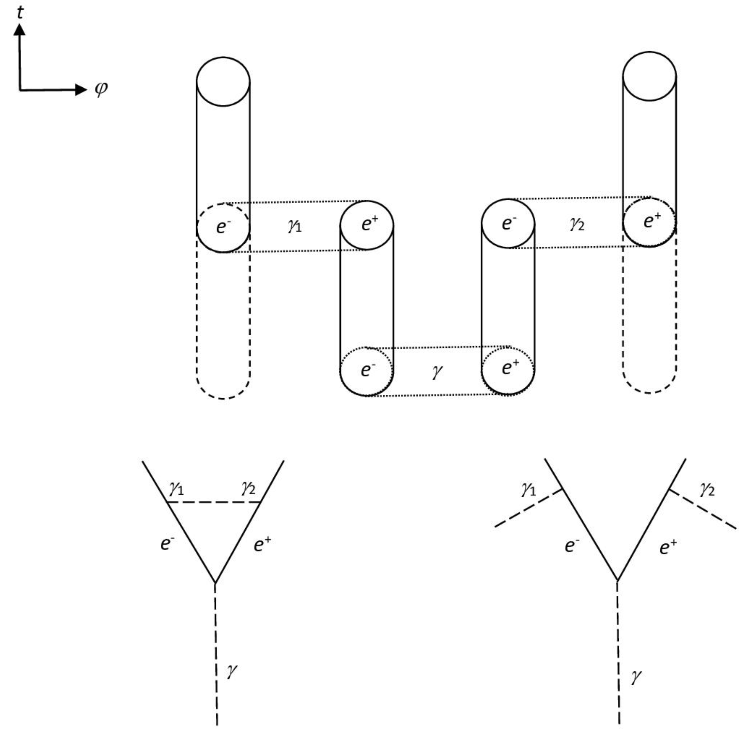
Figure 1. a) Absorption or emission of a photon by an electron (real process): the two processes are distinguished by the sign of the energy difference between the outgoing electron and the incoming electron; by exchanging electrons and positrons in the figure, the absorption or emission of the photon by a positron is obtained. b) Annihilation of an electron-positron pair (virtual process); by reversing the process around the horizontal axis, the analogous diagram for thecreation of a pair is obtained. The t-axis is time. The pairs generated by the dissociation of the photon are enclosed in horizontal tubes with dotted lines. The tubes delimited by continuous lines represent the states that evolve in t, those delimited by broken lines represent evanescent states associated with QJs. The elements of a given pair appear as separate for illustrative purpose only.

Figure 1. a) Absorption or emission of a photon by an electron (real process): the two processes are distinguished by the sign of the energy difference between the outgoing electron and the incoming electron; by exchanging electrons and positrons in the figure, the absorption or emission of the photon by a positron is obtained. b) Annihilation of an electron-positron pair (virtual process); by reversing the process around the horizontal axis, the analogous diagram for thecreation of a pair is obtained. The t-axis is time. The pairs generated by the dissociation of the photon are enclosed in horizontal tubes with dotted lines. The tubes delimited by continuous lines represent the states that evolve in t, those delimited by broken lines represent evanescent states associated with QJs. The elements of a given pair appear as separate for illustrative purpose only.

Figure 2. Decay of positronium into two photons (real process). On the right is the corresponding Feynman diagram, in which the horizontal variable is space. Note that while the internal fermionic line is not connected to evanescent states (due to QJs), the external fermionic lines are.

Figure 2. Decay of positronium into two photons (real process). On the right is the corresponding Feynman diagram, in which the horizontal variable is space. Note that while the internal fermionic line is not connected to evanescent states (due to QJs), the external fermionic lines are.

Figure 3. Decay of positronium into three photons (real process). On the right is the corresponding Feynman diagram, in which the horizontal variable is space. Note that while the internal fermionic lines are not connected to evanescent states (due to QJs), the external fermionic lines are.

Figure 3. Decay of positronium into three photons (real process). On the right is the corresponding Feynman diagram, in which the horizontal variable is space. Note that while the internal fermionic lines are not connected to evanescent states (due to QJs), the external fermionic lines are.

Figure 4. Photon dissociation (virtual process). The corresponding Feynman diagram is shown on the right, where the horizontal variable is space. The fermionic lines, being internal, are not connected to evanescent states.

Figure 4. Photon dissociation (virtual process). The corresponding Feynman diagram is shown on the right, where the horizontal variable is space. The fermionic lines, being internal, are not connected to evanescent states.

Figure 5. Two processes represented by the same state connection diagram, but by different Feynman diagrams, respectively in the case in which γ₁ and γ₂ are the extremes of the same photon line (left) or not (right).

Figure 5. Two processes represented by the same state connection diagram, but by different Feynman diagrams, respectively in the case in which γ₁ and γ₂ are the extremes of the same photon line (left) or not (right).

3.4. A Hypothesis on the Meaning of the De Vries Formula

We now want to show how a purely empirical formula proposed many years ago to express the renormalized fine structure constant can be interpreted in the present conceptual framework. We therefore specialize in the particular case in which the gauge boson B is the photon. To fix the ideas, we can make the identification, however not essential, (a, b) = (e⁺, e^-). As we have seen, the interaction is subordinate to the condition A = h/2 ± q²/c, where A is a random variable whose density is expressed by (104). The coupling constant must therefore contain the ratio between the probability of this fluctuation and the probability of a fluctuation of equal amplitude in the vacuum (A = 0):

$${\displaystyle \frac{\mathit{Probability}\hspace{0.17em}\left[A\hspace{0.17em}\hspace{0.17em}\in \hspace{0.17em}\hspace{0.17em}\left[\frac{h}{2}\hspace{0.17em}\hspace{0.17em}\pm \hspace{0.17em}\hspace{0.17em}\frac{q^2}{c}\right]\right]}{\mathit{Probability}\hspace{0.17em}\left[A\hspace{0.17em}\hspace{0.17em}\in \hspace{0.17em}\hspace{0.17em}\left[0\hspace{0.17em}\hspace{0.17em}\pm \hspace{0.17em}\hspace{0.17em}\frac{q^2}{c}\right]\right]}}\hspace{0.17em}\hspace{0.17em}\hspace{0.17em}\hspace{0.17em}\hspace{0.17em}\cong \hspace{0.17em}\hspace{0.17em}\hspace{0.17em}\hspace{0.17em}\hspace{0.17em}{\displaystyle \frac{\frac{1}{\sqrt{2\pi }}\hspace{0.17em}{e}^{-\hspace{0.17em}\frac{1}{2}\hspace{0.17em}{\left(\frac{h/2}{\hslash }\right)}^2}\cdot \hspace{0.17em}\hspace{0.17em}2\cdot \hspace{0.17em}\frac{q^2}{\hslash c}}{\frac{1}{\sqrt{2\pi }}\hspace{0.17em}\hspace{0.17em}\cdot \hspace{0.17em}2\cdot \hspace{0.17em}\frac{q^2}{\hslash c}}}\hspace{0.17em}\hspace{0.17em}\hspace{0.17em}=\hspace{0.17em}\hspace{0.17em}\hspace{0.17em}{e}^{-\hspace{0.17em}{\displaystyle \frac{{\pi }^2}{2}}}\hspace{0.17em}$$

(112)

Since the flavors a and b are identical to the flavors of the afferent fermions at the vertex by virtue of (101), and therefore the de Sitter radii of a and b are fixed by the conditions external to the vertex, the exchange of squared charge between a (b) and x (y) determines an exchange of mass by effect of (36). This exchange will be oriented: a will yield mass to x or vice versa, and the same will happen for b and y.

Since the charges of the two fermions a, b are equal in modulus and opposite in sign, the two exchange processes will be symmetric. Since q² is the total squared charge exchanged, each of the two fermions will exchange a squared charge equal to q²/2. The exchange of action implied in each of these two charge exchanges will be q²/2c. From Eq.(101), the total exchange of action in the dissociation process is h/2; thecoupling constant of the single element of the pair (a or b) is therefore:

$${\displaystyle \frac{q^2}{2c}}\hspace{0.17em}\hspace{0.17em}:\hspace{0.17em}\hspace{0.17em}\hspace{0.17em}{\displaystyle \frac{h}{2}}\hspace{0.17em}\hspace{0.17em}\hspace{0.17em}\hspace{0.17em}\hspace{0.17em}=\hspace{0.17em}\hspace{0.17em}\hspace{0.17em}\hspace{0.17em}\hspace{0.17em}{\displaystyle \frac{q^2}{\hslash c}}\hspace{0.17em}\hspace{0.17em}\cdot \hspace{0.17em}\hspace{0.17em}{\displaystyle \frac{1}{2\pi }}\hspace{0.17em}$$

(113)

Let us now consider the exchange of squared charge between a and x, or between b and y. In each of the two cases, the q²/2π factor in (113) represents the squared charge transferred from one of the two fermions (let's say fermion 1) to the other. We will therefore indicate this quantity as q²_{1 → 2}. Fermion 2 will return a share q²_{2→ 1} = q²_{1 → 2}/2π of squared charge to fermion 1, again in accordance with expression (113) which is symmetric with respect to the direction of the exchange. The process is clearly iterative and we can set:

$$q_{i\hspace{0.17em}+\hspace{0.17em}1}^2\hspace{0.17em}\hspace{0.17em}\hspace{0.17em}=\hspace{0.17em}\hspace{0.17em}\hspace{0.17em}\hspace{0.17em}{\displaystyle \frac{q_i^2}{2\pi }}\hspace{0.17em}\hspace{0.17em}\hspace{0.17em}\hspace{0.17em}\hspace{0.17em}$$

(114)

where i is the iteration index. Eq.(114) can be written in the form:

$$q_i^2\hspace{0.17em}\hspace{0.17em}\hspace{0.17em}=\hspace{0.17em}\hspace{0.17em}\hspace{0.17em}\hspace{0.17em}{\displaystyle \frac{q_0^2}{{\left(2\pi \right)}^i}}\hspace{0.17em}\hspace{0.17em}\hspace{0.17em}\hspace{0.17em}\hspace{0.17em}$$

(115)

This means that at the i-th iteration the coupling constant is α/(2π)ⁱ. The contribution of the i-th iteration to the overall coupling constant of the whole sequence of iterations is given by the product of α/(2π)ⁱ by the total contribution of the previous iterations. That is:α(i + 1) = α(i)α/(2π)ⁱ, where i = 0, 1, 2, 3... andα(0) = 1. We then have α(1) = α(0)α/(2π)⁰ = α, as is natural; α(2) = α(1)α/(2π)¹ = α²/2π ; α(3) = α(2)α/(2π)² = α³/(2π)³; α(4) = α(3)α/(2π)³ = α⁴/(2π)⁶, and so on. For each of the two sequences of iterations relating respectively to the exchanges between a and x, and between b and y, we therefore have a total coupling constant defined by the series:

$$\Gamma \left(\alpha \right)\hspace{0.17em}\hspace{0.17em}=\hspace{0.17em}\hspace{0.17em}1\hspace{0.17em}\hspace{0.17em}+\hspace{0.17em}\hspace{0.17em}{\displaystyle \frac{\alpha }{{\left(2\pi \right)}^0}}\hspace{0.17em}\left\{\hspace{0.17em}1\hspace{0.17em}\hspace{0.17em}+\hspace{0.17em}\hspace{0.17em}{\displaystyle \frac{\alpha }{{\left(2\pi \right)}^1}}\hspace{0.17em}\left[\hspace{0.17em}1\hspace{0.17em}\hspace{0.17em}+\hspace{0.17em}\hspace{0.17em}{\displaystyle \frac{\alpha }{{\left(2\pi \right)}^2}}\hspace{0.17em}\left(\hspace{0.17em}1\hspace{0.17em}\hspace{0.17em}+\hspace{0.17em}\hspace{0.17em}{\displaystyle \frac{\alpha }{{\left(2\pi \right)}^3}}\hspace{0.17em}\hspace{0.17em}\cdots \right)\right]\right\}\hspace{0.17em}$$

(116)

The first term is related to the absence of exchanges between a and x (or between b and y), and it represents the total squared charge hc/2 not yet exchanged, but available in the process B→ (a, b) [Eq.(101)].

The overall coupling constant is therefore the product of the two functions Γ(α), associated respectively with the two sequences, and the factor exp(-π²/2), that is α' = [Γ(α)]²exp(-π²/2). This must therefore be the coupling constant of the photon to the charged fermion. But this constant must equate α. We therefore have α' = α and hence:

$$\alpha \hspace{0.17em}\hspace{0.17em}=\hspace{0.17em}\hspace{0.17em}{\left[\Gamma \left(\alpha \right)\right]}^2\hspace{0.17em}{e}^{-\hspace{0.17em}{\displaystyle \frac{{\pi }^2}{2}}}\hspace{0.17em}$$

(117)

This relation defines the value of α. It was proposed, without any physical justification, by Hans De Vries more than twenty years ago [36]. We note that if z is the charge q_f of the fermion with which the photon couples, expressed in units e, i.e. z = q_f/e, the Eq.(117) actually does not give α but α/z². That is:

$${\displaystyle \frac{\alpha }{z^2}}\hspace{0.17em}\hspace{0.17em}\hspace{0.17em}=\hspace{0.17em}\hspace{0.17em}\hspace{0.17em}{\displaystyle \frac{1}{137,\hspace{0.17em}\hspace{0.17em}\mathrm{...}}}\hspace{0.17em}\hspace{0.17em}\hspace{0.17em}\hspace{0.17em}\hspace{0.17em}\Rightarrow \hspace{0.17em}\hspace{0.17em}\hspace{0.17em}\hspace{0.17em}\hspace{0.17em}\alpha \hspace{0.17em}\hspace{0.17em}=\hspace{0.17em}\hspace{0.17em}{\displaystyle \frac{z^2}{137,\hspace{0.17em}\mathrm{...}}}\hspace{0.17em}\hspace{0.17em}$$

(118)

as it should be. However, in common usage α is defined as 1/137,... and the coupling constant then becomes: z²α = z²/137,... .

The Eq.(117) can be solved iteratively by assigning an initial value to α and inserting it in the right-hand side, then substituting the value thus obtained again in the right-hand side and so on. The obtained value and the experimental one are reported below [37]:

CODATA 2018 (source: NIST): 7.297 352 5693(11) × 10^-3

Hans de Vries: 7.297 352 5686 × 10^-3

We must however point out that the CODATA 2022 adjustment differs from the computed result by 4 standard deviations (new recommended figure: 7.297 352 5643(11) × 10^-3) [38].

3.5. Mixing Matrices

Eq.(111) is inclusive of flavour mixing. We now want to investigate this phenomenon in the context of the present model. Let us consider the dissociation B → $q_1\hspace{0.17em}+\hspace{0.17em}{\overline{q}}_2$of a gauge boson B into two fermions of flavour a, b and charge q₁, -q₂ respectively. If B is self-conjugated, the self-conjugation property must extend to the pair ($q_1\hspace{0.17em},\hspace{0.17em}{\overline{q}}_2$); this is only possible if a = b and q₁ = q₂. This is the situation for B = H₀, γ, Z₀, graviton; hence the interactions of these bosons do not exhibit flavour mixing. In the case of gluons, the exchange of flavours a, b in the quark-antiquark pair ($q_1\hspace{0.17em},\hspace{0.17em}{\overline{q}}_2$) is equivalent to a charge conjugation. But the exchange of flavors cannot induce a modification of the color charge, given the ontological independence of color from flavor. This contradiction can be resolved only by imposing the equality a = b of flavors and therefore the absence of flavor mixing in interactions mediated by gluons. This leaves only the case of the W boson mediating weak interactions with charged currents. As in the gluonic case, the exchange of flavors a, b inverts the charge of the W. But, unlike the gluonic case, the electric charge is not ontologically independent of flavor; on the contrary, it is a function of it. Therefore there are no a priori reasons to assume the absence of flavor mixing in interactions mediated by the W.

Let us consider a virtual interaction vertex in which a W could couple with two fermions, one of generation i_a, the other of generation i_b. A fermion of generation i_a (i_b) would then enter this vertex and a fermion of generation i_b (i_a) would exit it. If we fix the difference n = | i_a – i_b |, there will be n + 1 possible entering states and the same number of exiting states, and therefore N = (n +1)² distinct modes of coupling between entry and exit. If we assign an arbitrary direction to each coupling, there will therefore be N² distinct pairs of couplings of opposite direction or “loops”. The real dissociation of the W, induced by the external fermionic lines of flavor a, b, selects one of these loops, consisting respectively of the coupling a → b (b → a) and the coupling b → a (a → b). A loop on N² is thus selected, which implies that the vertex amplitude is weighted by a factor 1/N. From now on we will consider the case of a real dissociation B → $q_1\hspace{0.17em}+\hspace{0.17em}{\overline{q}}_2$.

We must now construct the vertex amplitude (except for the factor constituted by the coupling constant, independent of a and b, which does not interest us here). The first factor that enters into this amplitude is clearly the product of the phase factors of the fermions originating from the dissociation of the W, which we will write:

$$e^{-i\hspace{0.17em}{\displaystyle \frac{m_a{c}^2}{\hslash }}\hspace{0.17em}\hspace{0.17em}{\displaystyle \frac{h}{M_W{c}^2}}\hspace{0.17em}\hspace{0.17em}+\hspace{0.17em}\hspace{0.17em}i\hspace{0.17em}{\displaystyle \frac{m_b{c}^2}{\hslash }}\hspace{0.17em}\hspace{0.17em}{\displaystyle \frac{h}{M_W{c}^2}}}\hspace{0.17em}\hspace{0.17em}\hspace{0.17em}\hspace{0.17em}=\hspace{0.17em}\hspace{0.17em}\hspace{0.17em}\hspace{0.17em}{e}^{-2\pi i\hspace{0.17em}{\displaystyle \frac{m_a}{M_W}}\hspace{0.17em}\hspace{0.17em}+\hspace{0.17em}2\pi i\hspace{0.17em}{\displaystyle \frac{m_b}{M_W}}}$$

(119)

Here m_a, m_b are the masses of the fermions of flavor a, b with which the W couples at the considered vertex; the time interval h/M_Wc², where M_W is the mass of the W, is the renormalization time scale of the W. A subsequent factor will contain the Wick-rotated versions of the wave functions of the outer fermions [Eqs. (46),(47)]:

$$e^{-\hspace{0.17em}{\xi }_a\hspace{0.17em}\hspace{0.17em}-\hspace{0.17em}\hspace{0.17em}\hspace{0.17em}{\xi }_b\hspace{0.17em}\hspace{0.17em}\hspace{0.17em}\hspace{0.17em}-\hspace{0.17em}\hspace{0.17em}i\hspace{0.17em}{\displaystyle \frac{Max(m_a,m_b)c^2}{\hslash }}\hspace{0.17em}{\displaystyle \frac{i\hslash }{M_W{c}^2}}\hspace{0.17em}\hspace{0.17em}\hspace{0.17em}+\hspace{0.17em}\hspace{0.17em}i\hspace{0.17em}{\displaystyle \frac{Min(m_a,m_b)c^2}{\hslash }}\hspace{0.17em}{\displaystyle \frac{i\hslash }{M_W{c}^2}}}\hspace{0.17em}\hspace{0.17em}\hspace{0.17em}\hspace{0.17em}=\hspace{0.17em}\hspace{0.17em}\hspace{0.17em}\hspace{0.17em}\hspace{0.17em}{e}^{-\hspace{0.17em}{\xi }_a\hspace{0.17em}\hspace{0.17em}-\hspace{0.17em}\hspace{0.17em}\hspace{0.17em}{\xi }_b\hspace{0.17em}\hspace{0.17em}\hspace{0.17em}\hspace{0.17em}\hspace{0.17em}+\hspace{0.17em}{\displaystyle \frac{\left|m_a\hspace{0.17em}\hspace{0.17em}-\hspace{0.17em}\hspace{0.17em}{m}_b\right|}{M_W}}}$$

(120)

The larger masses are considered to be incoming [with this choice, the action (incoming mass – outgoing mass)c² × ħ/M_wc² is positive and corresponds to the exponent in (120)]. The constants C of the exponentials in ξ_a,_b [Eq. (47)] have been assumed equal to 1, in accordance with what was established in Section 2.5. In accordance with the reasoning given at the end of Section 2.3, we then set ξ_a,_b = r/r_a,b = c| t |/r_a,b, where the variable r has the dimensions of a length and therefore the variable t has the dimensions of a time; r_a, r_b are the de Sitter radii of the fermions of flavor a, b; c is the limit speed. We will normalize the Wick-rotated wave functions y = Aexp(-c|t|/r_dS) according to the condition:

$${\displaystyle \underset{0}{\overset{\infty }{\int }}{\left|y\hspace{0.17em}\right|}^2}d\left|t\right|\hspace{0.17em}\hspace{0.17em}\hspace{0.17em}\hspace{0.17em}=\hspace{0.17em}\hspace{0.17em}\hspace{0.17em}\hspace{0.17em}1\hspace{0.17em}\hspace{0.17em}\hspace{0.17em}\hspace{0.17em}\hspace{0.17em}\hspace{0.17em}\hspace{0.17em}\hspace{0.17em}\Rightarrow \hspace{0.17em}\hspace{0.17em}\hspace{0.17em}\hspace{0.17em}\hspace{0.17em}\hspace{0.17em}\hspace{0.17em}\hspace{0.17em}\hspace{0.17em}A\hspace{0.17em}\hspace{0.17em}=\hspace{0.17em}\hspace{0.17em}\sqrt{{\displaystyle \frac{2c}{r_{dS}}}}\hspace{0.17em}\hspace{0.17em}\hspace{0.17em}$$

(121)

Integrating over the variable | t | we have:

$$S_{a,b}\hspace{0.17em}\hspace{0.17em}\hspace{0.17em}\hspace{0.17em}=\hspace{0.17em}\hspace{0.17em}\hspace{0.17em}\hspace{0.17em}\hspace{0.17em}\sqrt{{\displaystyle \frac{2c}{r_a}}}\hspace{0.17em}\hspace{0.17em}\sqrt{{\displaystyle \frac{2c}{r_b}}}\hspace{0.17em}\hspace{0.17em}{\displaystyle \underset{0}{\overset{\infty }{\int }}{e}^{-\hspace{0.17em}\frac{c\left|t\right|}{r_a}\hspace{0.17em}\hspace{0.17em}-\hspace{0.17em}\hspace{0.17em}\hspace{0.17em}\frac{c\left|t\right|}{r_b}\hspace{0.17em}\hspace{0.17em}\hspace{0.17em}\hspace{0.17em}}d\left|t\right|\hspace{0.17em}\hspace{0.17em}\hspace{0.17em}}=\hspace{0.17em}\hspace{0.17em}\hspace{0.17em}{\displaystyle \frac{2}{\sqrt{r_a{r}_b}}}\hspace{0.17em}\hspace{0.17em}\hspace{0.17em}{\displaystyle \frac{r_a{r}_b}{r_a\hspace{0.17em}\hspace{0.17em}+\hspace{0.17em}\hspace{0.17em}{r}_b}}\hspace{0.17em}\hspace{0.17em}$$

(122)

The integration is limited to positive values ​​of the scalar field ξ, which can be admitted if this variable is considered as an rms value of the field. The amplitude of the coupling vertex between the W and the two fermions is then expressed by:

$$f_{a,b}\hspace{0.17em}\hspace{0.17em}\hspace{0.17em}=\hspace{0.17em}\hspace{0.17em}\hspace{0.17em}{\displaystyle \frac{S_{a,b}\hspace{0.17em}\hspace{0.17em}\hspace{0.17em}{e}^{\frac{\left|m_a\hspace{0.17em}\hspace{0.17em}-\hspace{0.17em}\hspace{0.17em}{m}_b\right|}{M_W}}}{{\left(1\hspace{0.17em}\hspace{0.17em}+\hspace{0.17em}\hspace{0.17em}\left|i_a\hspace{0.17em}\hspace{0.17em}-\hspace{0.17em}\hspace{0.17em}{i}_b\right|\right)}^2}}\hspace{0.17em}\hspace{0.17em}{e}^{-2\pi i\hspace{0.17em}{\displaystyle \frac{m_a}{M_W}}\hspace{0.17em}\hspace{0.17em}+\hspace{0.17em}2\pi i\hspace{0.17em}{\displaystyle \frac{m_b}{M_W}}}$$

(123)

In the absence of mixing, we have a ≡ b and therefore, as can be easily seen, f_ab = δ_ab; the vertex amplitude is then reduced to the coupling constant. In the case of W, however, f is neither the unit matrix nor a diagonal matrix, and the problem therefore arises of how it can be diagonalized. As can be seen, the matrix f is Hermitian, that is (f_ab)* = f_ba. Let us consider the matrix V that diagonalizes the matrix f_ab, that is, such that VfV^-1 = Diag is diagonal. We immediately have (VfV^-1)⁺ = (V^-1)⁺f⁺(V)⁺ = (V^-1)⁺f(V)⁺ = (Diag)⁺ = Diag = VfV^-1, from which it follows that V is unitary. In the basis where f is diagonal, the W dissociates into one of three fermion-antifermion pairs. In the case of quarks these three pairs will be (d’, u), (s’, c), (b’, t) or (d, u’), (s, c’), (b, t’); in the following we will limit ourselves to the first case. The amplitudes d’, s’, b’are linear combinations of the amplitudes d, s, b and therefore there is flavor mixing. The matrix V is the mixing matrix. A similar reasoning applies to the dissociations of the W into leptonic a, b states (charged lepton and neutrino). The mixing matrix will be the CKM matrix for quarks, the PMNS matrix for leptons.

The relations presented in this section allow us to define the elements of the f_a,b matrix for both quarks and leptons (we will assume that the de Sitter radius of a neutrino mass eigenstate is the same as that of the charged lepton of the same generation). The correctness of the reasoning is then verified if the mixing matrix constituted by the best fit of the experimental data diagonalizes the f_a,b matrix for suitable choices of the fermion masses. Both the quark and neutrino masses are in fact known within experimental error bars, and the diagonalization will be better approximated by suitable choices of the values of these masses within the respective error bars. The situation is exposed in the next two subsections.

3.5.1. The CKM (Cabibbo-Kobayashi-Maskawa) Matrix

The calculation strategy is as follows. We start from the mixing matrix in the “standard” parametrization [39]:

$$V\hspace{0.17em}\hspace{0.17em}\hspace{0.17em}\hspace{0.17em}\hspace{0.17em}=\hspace{0.17em}\hspace{0.17em}\hspace{0.17em}\hspace{0.17em}\hspace{0.17em}\hspace{0.17em}\left(\begin{array}{ccc}{c}_{12}{c}_{13}& s_{12}{c}_{13}& s_{13}{e}^{-i{\delta }_{13}}\\ -s_{12}{c}_{23}-c_{12}{s}_{23}{s}_{13}{e}^{i{\delta }_{13}}& c_{12}{c}_{23}-s_{12}{s}_{23}{s}_{13}{e}^{i{\delta }_{13}}& s_{23}{c}_{13}\\ s_{12}{s}_{23}-c_{12}{c}_{23}{s}_{13}{e}^{i{\delta }_{13}}& -c_{12}{s}_{23}-s_{12}{c}_{23}{s}_{13}{e}^{i{\delta }_{13}}& c_{23}{c}_{13}\end{array}\right)\hspace{0.17em}\hspace{0.17em}\hspace{0.17em}$$

(124)

where c_ij = cos(θ_ij), s_ij = sin(θ_ij), (i, j) = 1, 2, 3. The matrix V is therefore entirely determined by the angles θ_ij and the phase δ₁₃. For these parameters we assume the experimental best fit values [39]:

θ₁₂ = 13.04° ± 0.05°    θ₂₃ = 2.38° ± 0.06°    θ₁₃ = 0.201° ± 0.011°    δ₁₃ = 68.08° ± 4.5°

Running the quark masses on their experimental error bars [40]:

m_u = 1.9-2.6 MeV    m_d = 3.5-5.5 MeV    m_s = 84-104 MeV

m_c = 1.15-1.35 GeV m_b = 4.2-4.4 GeV    m_t = 172 GeV (fixed)

we first compute the matrix f_ab, then the matrix VfV^-1 = Diag, choosing the values of the masses that minimize the ratio between the sum of the moduli of the off-diagonal terms of Diag and the sum of the moduli of its diagonal terms. The lowest value of this ratio (0.0039) is obtained with the following masses:

m_u= 1.97 MeV      m_d = 3.5 MeV      m_s = 84 MeV

m_c = 1.15 GeV       m_b = 4.2 GeV       m_t = 172 GeV (fixed)

The list of elements of Diag, defined up to a common factor, is as follows (for each element the real part is reported first, then the imaginary part):

Diag(1,1) = (9.907985479E-02, 4.445020854E-02)

Diag(1,2) = (-2.097622026E-03, 1.963231713E-03)

Diag(1,3) =(2.270226367E-03,    -1.590122236E-03)

Diag(2,1) =(8.128318004E-04,    2.398663666E-03)

Diag(2,2) = (0.134869426,       4.873338714E-02)

Diag(2,3) =(-9.121133015E-03,   1.912320405E-02)

Diag(3,1) =(1.110927667E-03,    -1.323248027E-03)

Diag(3,2) = (2.465872327E-03,    -8.105657063E-03)

Diag(3,3) = (0.766050756,       -9.318360686E-02)

These results are consistent with the proposal of this paper, that the mixing matrix V is the diagonalization matrix of the vertex amplitudes f_ab, obtained by postulating the dissociation of the gauge boson, induced by the act of interaction with the fermions with which it couples. The boson instead remains undissociated during its propagation.

3.5.2. The PMNS (Pontecorvo-Maki-Nakagawa-Sakata) Matrix

The procedure is the same as in the case of quarks. The matrix is ​​considered in the same standard parametrization seen in the previous subsection, with the following parameter values [41]:

θ₁₂ = 33.41° + 0.75° - 0.72°   θ₂₃ = 49.1° + 1.0° -1.3°   θ₁₃ = 8.54° +42° - 25°  δ₁₃ = 197° + 42° - 25°

Precisely, the central value is taken. The variation of the parameters within their error bars is not considered, leaving this possibility to possible future investigations. The masses of the charged leptons are considered fixed, while those of the neutrino mass eigenstates are varied within reasonable error bars, according to the following scheme(compatible with PDG limits):

m_e = 0.511 MeV    m_μ = 105.658 MeV    m_τ = 1776 MeV

m_ν1 = 0.0001-0.0006 eV    m_ν2 = 0.0001-0.001 eV    m_ν3 = 0.0001-0.06 eV

The lowest value of the ratio of the sum of the moduli of the off-diagonal terms of Diag to the sum of the moduli of its diagonal terms (0.1257) is obtained with the following masses:

m_ν1 = 0.0006 eV    m_ν2 = 0.001 eV    m_ν3 = 0.06 eV

that is, practically the upper extremes of the adopted bars. The list of the corresponding Diag elements is the following:

Diag(1,1) = (0.318358690,       4.858494736E-03)

Diag(1,2) = (2.038531750E-02, 1.348413900E-02)

Diag(1,3) = (1.689680666E-02,    -1.703028567E-02)

Diag(2,1) = (1.838763803E-02,    1.354285795E-02)

Diag(2,2) = (0.313012689,      7.760077715E-04)

Diag(2,3) = (-3.567337990E-04,    1.792673953E-02)

Diag(3,1) = (1.815088838E-02,    -1.137212384E-02)

Diag(3,2) = (1.312024891E-03,    1.500429027E-02)

Diag(3,3) = (0.368628621,      -5.634509027E-03)

It can therefore be stated that the calculation methodology illustrated in this Section also works in the case of leptonic couplings of the W boson. The results seem consistent with a direct mass hierarchy (although this point should be explored with more extensive numerical studies). In the calculation, the identity of the de Sitter radii of the states ν₁, ν₂, ν₃, and of the charged states e, μ, τ, respectively, has been assumed.

4. Conclusions

In these conclusions we would like to summarize in points, from a bird's eye view, the topics touched upon in the various sections of the article. The first hypothesis presented in this work is related to the vacuum of the Higgs field: it is associated with a field of de Sitter (dS) spaces tangent, at each point-event, to spacetime. The characteristics of these spaces (de Sitter radius, cosmological constant, gravitational constant, average density of matter-energy) are defined by the VEV and the mass of the Higgs boson. We then hypothesized that elementary particles are also fields of dS spaces on spacetime, whose properties are defined starting from the renormalized charge and mass of the specific particle.

The well-known Higgs mechanism, which provides mass to the elementary particles of the SM, can then be reinterpreted geometrically [4], in the sense that the field of dS spaces associated with an elementary particle derives from the field associated with the vacuum of the Higgs field through a rescaling of the internal gravitational constant. The latter has nothing to do with Newton's external gravitational constant, which governs the gravitational interactions between particles. In the context of this description, which is essentially pre-quantum (dS spaces are solutions of Einstein's gravitational equations in the internal cosmological constant), the spacetime coordinates are assimilable to degrees of freedom of the Higgs vacuum, inherited by the elementary particles in the rescaling process that constitutes the essence of the Higgs mechanism.

The quantum description is obtained by passing from Einstein's gravitational equations to their quantum counterpart, constituted by the WdW equation [19,20] (always in the internal cosmological constant). This passage imposes, as a consequence of the more general "time problem" [22,23] associated with this equation, the choice of an internal evolution variable of the dS spaces associated with a specific particle. It is possible to choose a variable that, in the Lorentzian regime, can be connected with the proper time of the particle. The harmonic quantum amplitudes in the proper time, solutions of the WdW equation, are the usual plane wave functions of the particle. They describe fields of dS spaces of definite mass and direction of the proper time axis (direction of the four-momentum), but completely indefinite position of the point of tangency on the spacetime. This results in the well-known quantum delocalization of elementary particles [6]. From the superposition of the plane wave functions thus constructed, with different time axes but the same mass (delocalization of the momentum) we obtain the general wave function of the particle, solution of the ordinary quantum-relativistic wave equations.

The Euclidean-time solutions of the WdW equation correspond, as usual in a third quantization scheme [42,43,44,45,46], to an evanescence of the field of dS spaces associated with a particle, or to its build up from the annihilation of previous states. The transition of a field of dS spaces from Lorentzian to Euclidean time, or vice versa, therefore models a quantum jump (QJ) [47,48]. QJs violate the unitarity of the evolution of the wave function, effectively implementing its “collapse”. The breaking of unitarity occurs at the level of micro-interactions between particles, without the participation of “environmental” degrees of freedom. This phenomenon is at the basis of classicalization [10,49].

A very important role is played by the local nature of interactions, consisting in the diagonality of the interaction operators on the basis of position. In a real event, i.e. associated with a QJ, the interacting particles are localized in the same spatial position (even if this can be delocalized in an interaction region of finite volume). The spatial degrees of freedom of matter then become the coordinates that express the position of real events (interaction regions) in a three-dimensional space independent of the particle indices. This fact becomes the decisive aspect of classicalization: macroscopic objects, which are not constituted by particles but by clusters of real interactions between particles, become stable entities in a three-dimensional space-arena external to them.

The nature of three-dimensional space as the geometric locus of real events of particle interaction is reflected in the existence of a positive cosmological constant. In fact, the localization of a positional eigenstate of a particle requires a concentration of energy in that space, around the position represented by the eigenvalues ​​of that eigenstate. This concentration of energy self-interacts gravitationally, and the minimum self-interaction energy corresponds to an infrared limit associated with a cosmological constant. The cosmological constant is therefore implied by the very property of space of being the locus where particle interactions are localized; it is completely independent of the zero-point energy of empty space. This explanation of the “small” value of the cosmological constant seems to be simpler than others based on arguments of a much more technical nature [50,51,52,53].

Finally, we investigated the interactions between elementary fermions and gauge bosons, proposing that in such interactions the bosons undergo a dissociation (or recombination), differently from their nature of non-composite entities manifested during free propagation. In this sense, gauge bosons are not associated with fields of dS spaces, unlike elementary fermions, but with dS spaces of fermion pairs originating from their dissociation at an interaction vertex.

This hypothesis – admittedly speculative – has at least two ramifications that have been discussed in detail. The first is the possibility of calculating the renormalized interaction constant starting from an analysis of the interaction process between the fermions originating from the dissociation of the boson and the external fermionic lines concurrent at the vertex. On this basis we have proposed, with reference to the case of the photon, a possible explanation for the formula proposed by De Vries for the calculation of the fine structure constant [36].

Second, in the case of an interaction vertex mediated by weak charged currents, the vertex amplitude comes to depend on the fermionic flavors. The unitary transformation of the fermionic states that diagonalizes the vertex amplitude then constitutes the mixing matrix. Preliminary numerical computations, reported in the paper, support this prediction for reasonable values ​​of the fermionic masses. It should be noted that the research program here only outlined, by indicating dependencies between the free parameters of the Standard Model (fermionic masses, interaction constants, mixing parameters) points in the direction of reducing the logical arbitrariness of the values ​​of these parameters, and thus of a future deeper theory of elementary particles.

Perhaps the most important aspect of the hypotheses discussed here is the emergence of a three-dimensional space-arena in the context of the classicalization process, and the unexpected role that the Higgs field would play in this process. The peculiarity of the Higgs field would no longer be only that of “giving mass to particles”, but also that of inducing their proper time (conjugated to the mass). The free evolution of massive particles is labelled by the proper time and, only to the accessory extent constituted by the delocalization of the momentum, also by the spatial position (conjugated to the momentum). QJs, and with them classicalization, would then be further aspects of this dynamical emergence of the spacetime ordering of real events. Removing the Higgs field from this process, we are left with a static space-arena, inhabited by matter alien to it in a sort of static, frozen, relation. This situation reproduces the background of the current theoretical representation. This paper can therefore be seen as a stimulus to overcome the traditional separation between spacetime and material fields; an overcoming somehow already announced by previous attempts, such as the Maldacena conjecture and holography [54,55].

References

- Higgs, P.W. Broken Symmetries and the Masses of Gauge Bosons. Phys. Rev. Lett. 1964, 13, 508. [CrossRef]
- Hamilton, M.J.D. Mathematical Gauge Theory.Chapter 8: The Higgs Mechanism and the Standard Model. Universitext Springer: Cham, Germany, 2017; pp. 445-526. [CrossRef]
- Navas, S. et al. (Particle Data Group). Status of Higgs Boson Physics. Phys. Rev. D 2024, 110, 030001. [CrossRef]
- De Sabbata, V.; Gasperini, M. Spontaneous symmetry breaking in a De Sitter metric background. Lett. Nuovo Cim. 1981, 31(7), 261-264. [CrossRef]
- Benza, V.; Caldirola, P. De Sitter microuniverse associated to the electron. Nuov. Cim. A 1981, 62, 175–185. [CrossRef]
- Chiatti, L. Quantum entities and the nature of time. Qeios 2023, 5UTZO4.2. [CrossRef]
- Von Neumann, J. Mathematical Foundations of Quantum Mechanics. Princeton University Press, Princeton, NJ, USA, 2018. ISBN:9780691178561.
- Christiaens, W. Non-spatiality and EPR-experiments according to the creation-discovery view. Found. Phys. Lett. 2003, 16(4), 379-387. [CrossRef]
- Baggott, J. The Quantum Cookbook: Mathematical Recipes for the Foundations for Quantum Mechanics. Oxford University Press, Oxford, UK, 2020. ISBN: 9780198827856.
- Crull, E.M. Quantum decoherence. In: The Rotledge Companion to Philosophy of Physics. Knox, A.; Wilson, A. Eds; Taylor and Francis Group, London, UK, 2021; Chapter 13. Online ISBN:9781315623818.
- Braghin, F.L. Linear sigma model at finite baryonic density and symmetry breakings. Braz. Journ Phys. 2007, 37(1a), 33-36. [CrossRef]
- Baym, G.; Grinstein, G. Phase transition in the σ model at finite temperature. Phys. Rev. D 1977, 15, 2897. [CrossRef]
- Recami, E. Multi-verses, micro-universes and elementary particles (hadrons). arXiv:physics/0505149.
- Recami, E.; Castorina, P. On quark confinement: hadrons as “strong black holes”. Lett. Nuovo Cim. 1976, 15(10), 347-350. [CrossRef]
- Moschella, U. The de Sitter and anti-de Sitter Sightseeing Tour. Séminaire Poincaré 2005, 1, 1-12. [CrossRef]
- Chiatti, L. Bit from Qubit. A Hypothesis on Wave-Particle Dualism and Fundamental Interactions. Information 2020, 11, 571. [CrossRef]
- Brindejonc, V.; Cohen-Tannoudji, G. An effective strong gravity induced by QCD. Mod. Phys. Lett. A 1995, 10(23), 1711-1718. [CrossRef]
- Kirchbach, M.; Compean, C.B. De Sitter special relativity as a possible reason for conformal symmetry and confinement in QCD. arXiv:1701.00450v2.
- Wheeler, J. A. Superspace and the Nature of Quantum Geometrodynamics. In: Topics in Nonlinear Physics. Zabusky, N.J. Ed.; Springer-Verlag, New York, NY, USA, 1969; pp 615-724.
- De Witt, B.S. Quantum Theory of Gravity I. The Canonical Theory. Phys. Rev. 1967, 160, 1113-1148. [CrossRef]
- Hartle, J.B.; Hawking, S.W. Wave function of the Universe. Phys. Rev. D 1983, 28, 2960-2975. [CrossRef]
- Kiefer, C.; Sandhöfer, B. Quantum Cosmology. arxiv.org/abs/0804.0672v2.
- Peres, A. Critique of the Wheeler-DeWitt equation. In: On the Einstein’s path; Harvey, A. Ed.; Springer, Berlin, Germany, 1999; pp. 367-379.
- de Broglie, L. Recherches sur la théorie de quanta. Ann. de Physique 1925, 10(3), 1-128.
- Hartman, T. Lecture Notes on Classical de Sitter Space. (accessed 08/02/2025). http://www.hartmanhep.net/GR2017/desitter-lectures-v2.pdf.
- Kompaneyets, A.S. Theoretical Physics. MIR, Moscow, USSR, 1961.
- Chiatti, L. Wave Function and Information. Quantum Rep. 2024, 6, 231–243. [CrossRef]
- Robles-Pérez, S.; Gonzáles-Díaz, P.F. Quantum state of the multiverse. Phys. Rev. D 2010, 81(8), 083529. [CrossRef]
- Nimmrichter, S. Classicalization and the Macroscopicity of Quantum Superposition States. In: Macroscopic Matter Wave Interferometry. Springer Theses, Springer, Cham, Germany, 2014. [CrossRef]
- Simonius, M. Spontaneous symmetry breaking and blocking of metastable states. Phys. Rev. Lett. 1978, 40, 980–983. [CrossRef]
- N. Aghanim et al. (Planck Collaboration). Planck 2018 results. VI Cosmological parameters. Astron. Astrophys. 2020, 641. [CrossRef]
- Penrose, R. The Emperor’s New Mind. Penguin Books, London, UK, 1989. ISBN: 0-19-851973-7.
- Chiatti, L; Licata, I. Particle Model from Quantum Foundations. Quant. Stud. Math. Found. 2017, 4, 181-204. [CrossRef]
- Kirchbach, M.; Popov, T.; Vallejo, J.A. The Conformal-Symmetry–Color-Neutrality Connection in Strong Interaction. In: Lie Theory and Its Applications in Physics. LT 2021. Dobrev, V. Ed.; Springer Proceedings in Mathematics & Statistics, vol 396. Springer, Singapore, 2021. [CrossRef]
- Chiatti, L. On the Thermomechanics of Hadrons and Their Mass Spectrum. Particles 2024, 7(4), 955-966. [CrossRef]
- De Vries, H. Available online: http://chip-architect.com/news/2004_10_04_The_Electro_Magnetic_coupling_constant.html (accessed 08/02/2025).
- Tiesinga, E.; Mohr, P.J.; Newell, D.B.; Taylor, B.N. CODATA recommended values of the fundamental physical constants: 2018. Rev. Mod. Phys. 2018, 93, 025010. [CrossRef]
- NIST 2024. https://physics.nist.gov/cgi-bin/cuu/Value?alph|search_for=fine+structure (accessed 08/02/2025).
- Ceccucci, A.; Ligeti, Z.; Sakai, Y. (PDG 2020). CKM quark-mixing matrix. https://pdg.lbl.gov › 2020 › reviews › rpp2020-rev-ckm-matrix.pdf. (accessed 08/02/2025).
- Manohar, A.V.; Lellouch, L.P.; Barnett, R.M. (PDG 2020). Quark masses. https://pdg.lbl.gov/2020/reviews/rpp2020-rev-quark-masses.pdf. (accessed 08/02/2025).
- PDG Group. https://pdglive.lbl.gov/Particle.action?node=S067&init=0 (accessed 08/02/2025).
- McGuigan, M. Third quantization and the Wheeler-DeWitt equation. Phys. Rev D 1988, 38(19), 3031-3051. [CrossRef]
- Robles -Pérez, S. J. Third quantization: modeling the universe as a ‘particle’ in a quantum field theory of the minisuperspace. Journ. Phys. Conf. Ser. 2013, 410, 012133. [CrossRef]
- Strominger, A. Baby universes. In: Quantum Cosmology and Baby Universes; Volume 7. Coleman, S.; Hartle, J.B.; Piran, T.; Weinberg, S. Eds.;World Scientific, London, UK, 1990. pp. 272-339.
- Giddings, S.B.; Strominger, A. Baby universe, third quantization and the cosmological constant. Nucl. Phys. B 1989, 321(2), 481-508. [CrossRef]
- De, S.S.; Rahaman, F.;Mapdar, A. Subatomic particle as the quantum universe. https://arxiv.org/abs/2002.02392.
- Bohr, N. On the Constitution of Atoms and Molecules. Philos. Mag. Ser. 1913, 6 (26), 1-25 (Part I), 476-502 (Part II), 857-875 (Part III).
- Heisenberg, W. Die Physikalischen Prinzipien der Quantentheorie. Hirzel, Leipzig, Germany, 1930.
- Castagnino, M.; Fortin, S.; Laura, R.; Sudarski, D. Interpretations of Quantum Theory in the Light of Modern Cosmology. Found. Phys. 2017, 47,1387–1422. [CrossRef]
- Rubakov, V.A. On third quantization and the cosmological constant. Phys. Lett B 1988, 214(4), 503–507. [CrossRef]
- Coleman, S. Why there is nothing rather than something? A theory of the cosmological constant. Nucl. Phys. B. 1988, 310, 643–668. [CrossRef]
- Barvinsky, A.O. Kamenshchik, A.Y. Cosmological landscape and Euclidean quantum gravity. Journ. Phys. A 2007, 40(25), 7043–7048. [CrossRef]
- Barvinsky, A.O. Why There is Something Rather than Nothing: Cosmological Constant from Summing over Everything in Lorentzian Quantum Gravity. Phys. Rev. Lett. 2007, 99, 071301. [CrossRef]
- Maldacena, J. The large N limit of superconformal field theories and supergravity. Adv. Theor. Math. Phys. 1998, 2, 231-252. [CrossRef]
- Susskind, L. The world as a hologram. J. Math. Phys. 1995, 36, 6377–6396. [CrossRef]
Disclaimer/Publisher’s Note: The statements, opinions and data contained in all publications are solely those of the individual author(s) and contributor(s) and not of MDPI and/or the editor(s). MDPI and/or the editor(s) disclaim responsibility for any injury to people or property resulting from any ideas, methods, instructions or products referred to in the content. |
© 2025 by the authors. Licensee MDPI, Basel, Switzerland. This article is an open access article distributed under the terms and conditions of the Creative Commons Attribution (CC BY) license (http://creativecommons.org/licenses/by/4.0/).
Copyright: This open access article is published under a Creative Commons CC BY 4.0 license, which permit the free download, distribution, and reuse, provided that the author and preprint are cited in any reuse.