
Submitted:
13 February 2025
Posted:
14 February 2025
You are already at the latest version
Abstract
The human functional connectome (FC) is a representation of the functional couplings between brain regions derived from blood oxygen level-dependent (BOLD) signals. We hypothesized that tensors, given their ability to project high-dimensional data into lower dimensional spaces via decomposition techniques, enable detecting the brain fingerprint with high accuracy. In this work, we present a mathematical framework based on Tucker decomposition to uncover the FC fingerprint of participants from the Young-Adult Human Connectome Project (HCP) Dataset. We analyzed how the following factors relate to within-and between-condition (rest-task) fingerprinting: brain parcellation granularity, decomposition rank, and scan length. Relative to FC matrices, we observed the highest increase in matching rates for parcellation granularity of 214 in the within-condition setting. Notably, our framework provides a substantial matching rate improvement in the between-condition setting relative to original FC matrices. Further, with our framework, sub-sampling the resting-state time series in the between-condition setting yielded fingerprinting results similar to those obtained by sampling the entire resting-state time series.
Keywords:
functional connectome
; tensor decomposition
; fingerprinting
; dimensionality reduction
1. Introduction
Human brain connectomics is a field of research that has emerged as a result of the large availability of neuroimaging datasets in recent years [1]. This field of study has the potential to answer many open questions about the structure and function of the human brain. Furthermore, connectomics based analyses have uncovered differences between healthy and disease conditions [2,3]. However, in order to further validate the reliability of such studies and deepen the understanding of individual characteristics that can be overlooked in cohort studies, the concept of a “brain connectivity fingerprint” [4,5,6] has gotten a lot of attention.
Functional connectivity fingerprinting of the brain refers to the ability to identify an individual FC from a set of FCs in repeated fMRI imaging sessions. The existence of a brain fingerprint has been established in the last decade with work done with data from functional magnetic resonance imaging (fMRI) and electroencephalography (EEG) [7,8]. Such studies have shown that the functional connectome (FC) of the brain varies between individuals, therefore serving to some extent as a fingerprint. In the literature, different studies of FC fingerprinting have been conducted with varying approaches, such as principal component analysis (PCA) [9,10], sparse dictionary learning (SDL) [11], geodesic distance in regularized FC [12] and correlation distance in FC tangent space projections [13]. In [9], the authors show that individual connectivity profiles can be reconstructed through an optimal linear combination of PCA-derived orthogonal components. In [10], the authors perform PCA in a subset of “learning” FCs to obtain an eigenspace to which the “validation” FCs are projected, thus enabling the identification of the fMRI condition or the participant to which the “validation” FC belongs. In [11], SDL is used to refine FC profiles, leading to a higher distinctiveness in FCs relative to raw connectivity. PCA and SDL work on 2-dimensional data, while Tucker decomposition is designed for higher-dimensional data structures called tensors, essentially allowing it to analyze complex relationships across multiple variables in a dataset by decomposing it into a core tensor and factor matrices along each dimension. In essence, Tucker decomposition may be thought of as a “higher-order PCA”.
Using the fact that FCs estimated as correlation matrices lie on or inside a Symmetric Positive Definite (SPD) manifold, Venkatesh and colleagues proposed using geodesic distance to compare FCs [14]. In a follow-up study [12], the authors explored how optimally regularized FCs maximize the individual fingerprint of participants, measured by the geodesic distance between their FCs. A limitation of this approach is that the geodesic distance between FCs of size is a map . Hence, even though the geodesic distance provides a global measure of similarity between FCs, it does not directly highlight the specific features that make the individual’s functional connectivity unique. As an alternative to using FCs, tangent FCs have demonstrated a high capacity to predict cognition and behavior [15,16,17]. Most recently, [13] analyzed the effects of tangent FCs with respect to fingerprinting. In that study, a high degree of fingerprinting was achieved not only for the test / retest sessions but also for the successful matching of twins.
To simultaneously overcome the drawbacks of the studies mentioned above, we propose to utilize tensor decomposition for FC fingerprinting. Tensor decomposition enables projecting high-dimensional data into a lower-dimensional space, preserving its structure while independently extracting meaningful information from each dimension.
Tensors are multidimensional arrays with applications in various fields, including signal processing, computer vision, and neuroscience [18]. In brain connectomics, tensors enable modeling and analyzing the functional and structural connections within the brain by reducing the dimensionality of complex, interrelated, and high-dimensional data through tensor decomposition. In [19], the authors studied the dynamics of FCs to understand the process of formation and dissolution of brain functional networks through tensor decomposition techniques. In another study [20], it was demonstrated how the analysis of the tensor components enables the extraction of unbiased and interpretable descriptions of single-trial dynamics across many trials through low-dimensional representations of neural data. In [21], the authors discuss challenges associated with interpreting the brain connectivity patterns derived from tensor decomposition. To our knowledge, only [22] has considered using tensors in brain connectivity fingerprinting analysis in the literature. However, their study was based on structural connectivity. The task of identifying subjects through their functional connectomes has the additional challenge of dynamic changes and functional reconfigurations happening at a fast rate in response to cognitive stimuli.
Our study assesses how tensor decomposition of functional connectivity is related to fingerprinting measured by matching rate [23]. Specifically, we used Tucker’s decomposition [24] to uncover brain fingerprints derived from FCs. Tucker decomposition decomposes a tensor into a core tensor and a set of n factor matrices, where n is the number of dimensions of the tensor. The core tensor can be thought of as a compressed version of the original tensor and the factor matrices as principal components along the n dimensions of the tensor. Considering the focus of brain fingerprinting of this study, the tensors here used were obtained by concatenating all participants’ functional connectivity matrices from one scanning session, thus resulting in three-dimensional tensors. Decomposing such tensors via Tucker decomposition yields a core tensor and three factor matrices, the first two of which capture cohort-level functional connectivity patterns, while the third captures participant-specific patterns. We used data from all fMRI conditions available in the Young-Adult Human Connectome Project (HCP) Dataset, which consists of two fMRI data acquisition sessions (referred to as test and retest throughout this paper) from 1200 participants. In particular, we focused on a subset of that dataset consisting of 426 unrelated participants. Our chosen measurement of fingerprinting was matching rate [23], which measures among participants how often (percentage of times) one session is correctly paired with another session (and vice versa).
The aims of this paper are: (i) assess the impact of Tucker decomposition on functional connectome fingerprinting in within- and between-fMRI condition settings for different parcellation granularities, (ii) estimate optimal levels of compression of brain parcellation-specific and participant-specific information that maximize fingerprinting, and (iii) analyze how sampling in resting-state prior to Tucker decomposition affects fingerprinting.
The remainder of the paper is organized as follows. In the [sec:data]Materials and Methods section, we: (i) describe the data set used in this study as well as the preprocessing procedures, (ii) provide a review of multilinear algebra and tensor decomposition algorithms, (iii) introduce Tucker decomposition, and (iv) describe matching rate, the fingerprinting measurement used in this study. In the [sec:results]Results section, we: (i) uncover fingerprinting within and between fMRI conditions, (ii) disclose optimal levels of compression of parcellation-specific and participant-specific information that maximize fingerprinting, and (iii) present the findings for the different strategies of sampling time points in resting-state time series. In the [sec:discussion]Discussion section, we (i) discuss our findings and provide possible interpretations of them and (ii) highlight some limitations of our study and make suggestions for future work.
2. Materials and Methods
2.1. Dataset
The data set used in this study consists of the eight fMRI conditions available in the Young-Adult HCP Dataset [25]. Specifically, we used a subset of 426 unrelated participants (223 women, mean age: 28.67 years, range: 22–36) to eliminate the need to account for potential hereditary factors that could have an influence on fingerprinting. fMRI conditions include: resting-state (RS), emotion processing (EP), gambling (GAM), language (LAN), motor (MOT), relational processing (REL), social cognition (SOC), and working memory (WM). For each condition, participants underwent two sessions corresponding to two different acquisitions (left-to-right, LR, and right-to-left, RL). In our study, we refer to these as test and retest sessions. The resting-state scans were acquired in four sessions (“REST1” and “REST2”) on two different days. Only the two sessions of REST1 were used in this work.
2.2. Brain Parcellations
In this work, we used the Schaefer parcellation functional brain atlases of the human cortex [26]. The Schaefer parcellation is based on resting-state fMRI data from 1489 participants, which were registered using surface alignment. The Schaefer parcellation was obtained via a gradient-weighted Markov random field that integrates local gradient and global similarity approaches and is available at ten granularity levels, ranging from 100 to 1000 in steps of 100 in both volumetric and grayordinate space. The grayordinate versions of the parcellations are in the same surface space as the HCP fMRI data, therefore, mapping the parcellations onto the fMRI data is trivial. Furthermore, using surface-mapping produces a better alignment between the fMRI data and the Schaefer parcellations in comparison to when volumetric mapping is used. Consequently, we used the surface-based mapping to map the 200, 400, and 800 granularity Schaefer parcellations onto the fMRI data. For completeness, 14 subcortical regions were added to each parcellation, as provided by the HCP release (filename Atlas_ROI2.nii.gz). To do so, this file was converted from NIFTI to CIFTI format using the HCP workbench software (www.humanconnectome.org/software/connectome-workbench.html, wb_command -cifti-createlabel). As a result, the Schaefer-200 parcellation, for example, ultimately contained 214 brain regions.
2.3. Preprocessing
A “minimal” preprocessing pipeline from the HCP, which includes artifact removal, motion correction, and registration to a standard template, was used [27]. More details can be found in the literature [28,29].
The “minimal” preprocessing pipeline was improved upon through the addition of extra steps. These steps were also described at [13]. For resting-state fMRI data we: (i) regressed out the global gray matter signal from the voxel time courses [27], (ii) applied a first-order Butterworth bandpass filter in the forward and the reverse directions [0.001–0.08Hz [27], functions butter and filtfilt in MATLAB], and (iii) z-scored and averaged, per brain regions, the voxel time courses, excluding any outlier time points falling outside three standard deviation from the mean (workbench software, wb_command -cifti-parcellate). The same steps were repeated for all fMRI tasks, however, a larger frequency range was used in the bandpass filter (0.001–0.250) [30], since the optimal range is unclear [31].
2.4. Estimation of Whole-Brain FCs
The functional connectivity between pairs of brain regions was estimated by computing Pearson’s correlation (corr MATLAB function), which results in a symmetric correlation matrix, with M being the number of brain regions for a given parcellation. Throughout this article, this correlation matrix is referred to as FC. For each participant, we computed a whole-brain FC for each of the two sessions (test and retest), each fMRI condition (all seven tasks and resting state), and different parcellation granularities (214, 414, and 814).
2.5. Tensor Notation and Linear Algebra
In this work, we refer to multidimensional arrays as tensors. The order of a tensor describes the number of dimensions it has. Zero-order tensors are scalars, first-order tensors are vectors, second-order tensors are matrices, and tensors of order three or higher are referred to as higher-order tensors. The tensor notation used in this paper is largely adapted from [18]. Throughout the paper, higher-order tensors are denoted by Euler script letters, e.g., , matrices are denoted by boldface capital letters, e.g., , vectors are denoted by boldface lowercase letters, e.g., , and scalars are denoted by lower or upper case letters, e.g., x or X. Entries of a matrix or a tensor are denoted by lowercase letters with subscripts, e.g., the entry of an N-order tensor is denoted by .
Equivalently to rows and columns from matrices, tensors have fibers. Fibers are constructed by fixing every index of the tensor, but one. Hence, tensors have as many fibers as dimensions. A matrix column is a mode-1 fiber, and a matrix row is a mode-2 fiber. This concept can also be extended to higher-order tensors. For instance, third-order tensors have column (mode-1), row (mode-2), and tube (mode-3) fibers, which are denoted by , , and , respectively. A slice is defined by fixing all entries from the tensor except two. For example, we can define the slices , , and for a third-order tensor.
An N-order tensor can be flattened into a matrix, a process known as matricization or flattening. The mode-n matricization of a tensor is denoted by and arranges the mode-n one-dimensional fibers to be the columns of the resulting matrix. The n-mode matrix product between a tensor and a matrix is denoted by and is of size .
The inner product of and is the sum of the product of their entries, i.e., The norm of tensor is defined as For matrices, refers to the Frobenius norm, and for vectors, refers to the analogous norm.
2.6. Tensor Decomposition
In recent years, tensors have become increasingly popular in the fields of signal processing, machine learning, and neuroscience for their capacity to model complex high-order relationships among objects [32,33,34]. Tensor decomposition enables projecting high-dimensional data into a lower-dimensional space while preserving the original structure of the data. For the purpose of brain fingerprinting, tensor decomposition has the potential of extracting unique features from each participant’s fMRI data acquisition session, thus facilitating subject distinctiveness. Several tensor decomposition algorithms can be found in the literature, each with their own characteristics and applications. The most commonly used ones are the CANDECOMP/PARAFAC (CP) [35,36] decomposition and the Tucker decomposition [24].
The CP decomposition factorizes a tensor into a sum of rank-one tensors, with a rank-one tensor being expressed by the outer product between vectors. For a N-order tensor , its CP decomposition is given by:
where R, which represents the number of rank-one tensors used to reconstruct the original tensor, is the rank of the decomposition, is a scaling constant for each of the components, and , for , are factor matrices. The last equality shows the shorthand introduced in [37].
The Tucker decomposition decomposes a tensor into a core tensor multiplied by a matrix along each of the tensor modes [24]. For , its n-rank, denoted by , is defined as the column rank of its mode-n matricization . In other words, the n-rank is the number of linearly independent vectors that span the basis of the mode-n fibers of . The Tucker decomposition of is defined as:
Here, , ⋯, are column-wise orthonormal matrices referred to as factor matrices, and are the ranks of the decomposition, where for . If ), we refer to the decomposition as a truncated Tucker decomposition and refer to it as a rank-() decomposition. The tensor is referred to as the core tensor and its entries represent the level of interaction between the different factors. Note that the CP decomposition can be understood as a special case of the Tucker decomposition when the Tucker’s core is reduced to a hyper-diagonal tensor (all non-diagonal entries are equal to zero) and . For simplicity, consider the third-order tensor . The Tucker decomposition of is the solution of the minimization problem:
2.7. Tucker Decomposition Of Functional Connectomes
For each of the eight fMRI conditions analyzed in this study, we represent the data as a third-order tensor . Here, M is equal to the granularity of the brain parcellation and corresponds to the total number of participants. Given the symmetry of FC matrices, we refer to as a semi-symmetric tensor, which is defined as invariant under permutation of two (or more) indices. In our case, for . All analyses performed in this work have an input of a semi-symmetric tensor constructed by concatenating participants’ FCs obtained in one fMRI scanning session (either test or retest).
Once the data have been structured as a semi-symmetric tensor, we can produce a low-rank estimation of the FCs through either of the previously mentioned tensor decomposition methods. Due to the lack of interactions between components, the results of CP decomposition are generally easier to interpret [21] compared to Tucker decomposition. However, this lack of interaction often leads CP to produce less accurate approximations of the original tensor, as measured by the norm. In contrast, Tucker decomposition leverages its core tensor to capture interactions between components, enabling it to approximate the original tensor with greater precision [38]. Considering the interpretability/accuracy trade-off in the context of brain fingerprinting, we focus on Tucker decomposition.
Several methods have been developed to estimate the Tucker decomposition. Here, we use the High-Order Singular Value Decomposition (HOSVD) [39]. HOSVD is an extension of the classic Singular Value Decomposition (SVD) to higher order arrays. Specifically, HOSVD factorizes a tensor into a core tensor and a set of column-wise orthogonal factor matrices. Similarly to PCA, the factor matrices capture most of the variance across each of the tensor modes. For a N-order tensor , the Tucker estimation via HOSVD is shown in Algorithm 1.
| Algorithm 1: Higher Order Singular Value Decomposition (HOSVD) |
|
Input:
Output:
|
When applied to tensors that exhibit partial (or full) symmetries, HOSVD preserves the symmetric structure of the tensor [39]. Hence, for a tensor consisting of one session (e.g., test sessions) of participants’ FC matrices, the Tucker decomposition of can be reformulated as:
where the factor matrices and obtained via HOSVD contain, respectively, brain parcellation and participant-specific information and the ranks and express the compression levels of brain parcellation and participant-specific information. For the parcellation granularities considered in this study (214, 414, and 814), the brain parcellation ranks were chosen with a step size of . In addition to the previous parcellation ranks, we also performed a full-rank decomposition. Thus, for a parcellation granularity of 414, for example, the brain parcellation ranks were set to . In contrast, all participant ranks were fixed and set to .
Under the hypothesis that the functional connectivity patterns of a participant are, to some extent, reproducible across scanning sessions, we fix the core tensor and brain parcellation factor matrix derived from the Tucker decomposition of tensor and estimate the participant factor matrix of the tensor comprising of FCs from another data acquisition session (e.g., retest session). By doing so, we aim to detect a consistent presence of underlying cohort-level functional connectivity patterns across different data acquisition sessions for each participant. Such a problem can be formulated as follows:
The above problem admits a closed-form solution given by:
where † denotes the Moore-Penrose inverse [40] of a matrix, and and denote the mode-3 matricization of and , respectively.
2.8. Fingerprinting Quantification
To quantify fingerprinting, we used a measure denominated matching rate [23] for an identifiability matrix , where denotes the Pearson’s correlation between the j-th row of the participant factor matrix , and the k-th row of the participant factor matrix . The main diagonal entries of represent similarity levels between different imaging sessions of the same participant. By hypothesis, we expect those entries to be higher than the off-diagonal entries, which represent the similarity level between different imaging sessions of different participants. Matching rate is a variation of [7] that accounts for the fact that each participant is present only once in the test and the retest sets. (1) is the average frequency at which a participant’s test session is most highly correlated to their retest session, and their retest session is most highly correlated to their test session (note that one does not necessarily imply the other). For matching rates, we impose that once a test session is paired with a retest session, it can no longer be chosen for a new pairing. The relative frequency of successful participants matching in both directions is then averaged, yielding a value in the range , where 0 indicates a failure to correctly match any of the participant’s FCs, and 1 indicates success in matching all participant’s FCs correctly. An algorithmic description of the computation of the matching rate is presented in Algorithm 2.
| Algorithm 2: Matching Rate Computation |
|
Input:
Output:
|
2.9. Fingerprinting Framework Adapted to Tucker Decomposition
Our fingerprinting framework consists of five key steps: i) given a data acquisition session (either test or retest) of an fMRI condition, construct a tensor that contains all participants FCs, ii) decompose the tensor via Tucker decomposition to obtain a core tensor, a brain parcellation factor matrix, and a participant factor matrix, iii) estimate the other session’s participant factor matrix based on the decomposition of the given session, iv) obtain an identifiability matrix by computing pairwise Pearson’s correlation between the rows of both participant factor matrices, and v) calculate the matching rate for the obtained identifiability matrix. A schematic representation of our framework is presented in Figure 1.
In the following section, we discuss how matching rate is affected by the rank of the decomposition, parcellation granularities, the scanning length of fMRI conditions, and under within- and between-condition scenarios.
3. Results
For all eight fMRI conditions, the proposed fingerprinting framework was applied to two main settings. First, when test and retest FCs correspond to the same fMRI condition (within-condition fingerprinting). Second, when combining resting-state FCs with task FCs (between-condition fingerprinting). For the aforementioned settings, we further investigated the impact of brain parcellation rank and participant rank on Tucker decomposition and subsequent fingerprinting, and whether scanning length duration has a significant effect on matching rates. Given that no significant increase in matching rate was observed when comparing parcellation granularity 414 to 814 in the within-condition analyses (see Figure 2), we restricted our between-condition analyses to parcellation granularity of 414.
3.1. Evaluating the Impact of Brain Parcellation Rank and Participant Rank on Fingerprinting
To obtain a holistic view of how brain parcellation rank and participant rank affect fingerprinting, we computed matching rates under different combinations of both ranks for all fMRI conditions. Results shown in Figure 3 indicate that higher brain parcellation ranks led to higher matching rates compared to lower brain parcellation ranks. However, the impact of the participant rank on matching rates depends on the fMRI condition. Specifically, with Emotion and Motor tasks we can achieve near-optimal matching rates with a participant rank of 300 or higher, while for all the other fMRI tasks we achieve near-optimal matching rates earlier, starting at participant rank of 150. Resting-state matching rates were the highest among all fMRI conditions, reaching optimal scores starting at participant rank 100, with 100% matching accuracy. In contrast, Emotion had the lowest matching rate.
3.2. Within-Condition Fingerprinting
The concept of within-condition fingerprinting reflects the ability to correctly match two scans of the same participant when all evaluated scans belong to the same fMRI condition. With our fingerprinting framework, we obtained a substantial increase in matching rate across all considered parcellation granularities relative to vectorized original FCs, which were adopted as baseline. For original FCs, identifiability matrices were obtained by computing pairwise Pearson’s correlation between test and retest vectorized upper triangular original FCs. In Figure 2, we show, for each condition, the highest matching rate obtained for all possible combinations of brain parcellation rank and participant rank. The highest matching rate increase with respect to original FCs was observed for parcellation granularity of 214, for which our framework generated an increase in fingerprinting accuracy ranging from 11% (Language) to 36% (Emotion). Resting-state matching rates were the highest in all parcellations, achieving 100% for all parcellation granularities. Our fingerprinting framework was carried out by inputting a tensor consisting of test FCs while estimating the participant’s factor matrix of a tensor consisting of retest FCs and vice versa. In this section, we report the averages between both procedures.
3.3. Between-Condition Fingerprinting
Between-condition fingerprinting measures the degree to which we can match, for each participant, a scan from one fMRI condition to their scan from another fMRI condition. Using our fingerprinting framework, we estimate the participant factor matrix from a tensor consisting of task (test) fMRI by inputting a tensor consisting of resting-state (retest) FCs. Given that the scanning length of resting-state is substantially longer than the length of all fMRI tasks, we consider two scenarios when estimating resting-state FCs: i) using the full resting-state time series and ii) matching (hence reducing) the number of timepoints in the resting-state time series to the duration of each task (e.g., when pairing with Emotion task, resting-state FCs are computed using 166 out of the total 1190 time points). In the latter case, we further explore two strategies for sampling time points of the resting-state scan: i) randomly sample time points, and ii) randomly sample a starting time point in the range of and take the randomly sampled starting time point and its consecutive time points.
3.3.1. Between-Condition Fingerprinting with Resting-State Full Scanning Length
The between-condition matching rates when resting-state FCs are estimated using the time series of the full scanning length are shown in Figure 4. Matching rates ranged from (Relational) to (Language). In Figure 4, we observe a high sensitivity to brain parcellation rank, with 414 being the optimal rank. Comparatively, matching rate also benefits from a higher participant rank. However, the degree to which this occurs is task dependent (i.e., a participant rank of 350 is nearly optimal for Emotion, but for Relational there is a clear benefit in going up to rank 426). In Figure 5, we observe a major increase in between-condition matching rates using Tucker decomposition when compared to original FCs. The procedure used for computing the identifiability matrix for original FCs in the between-condition setting was analogous to the one in the within-condition setting. Matching rate improvements obtained with Tucker ranged from 43% (Relational) to 72% (Language).
3.3.2. Between-Condition Fingerprinting with Resting-State Matched-to-Task Scanning-Length
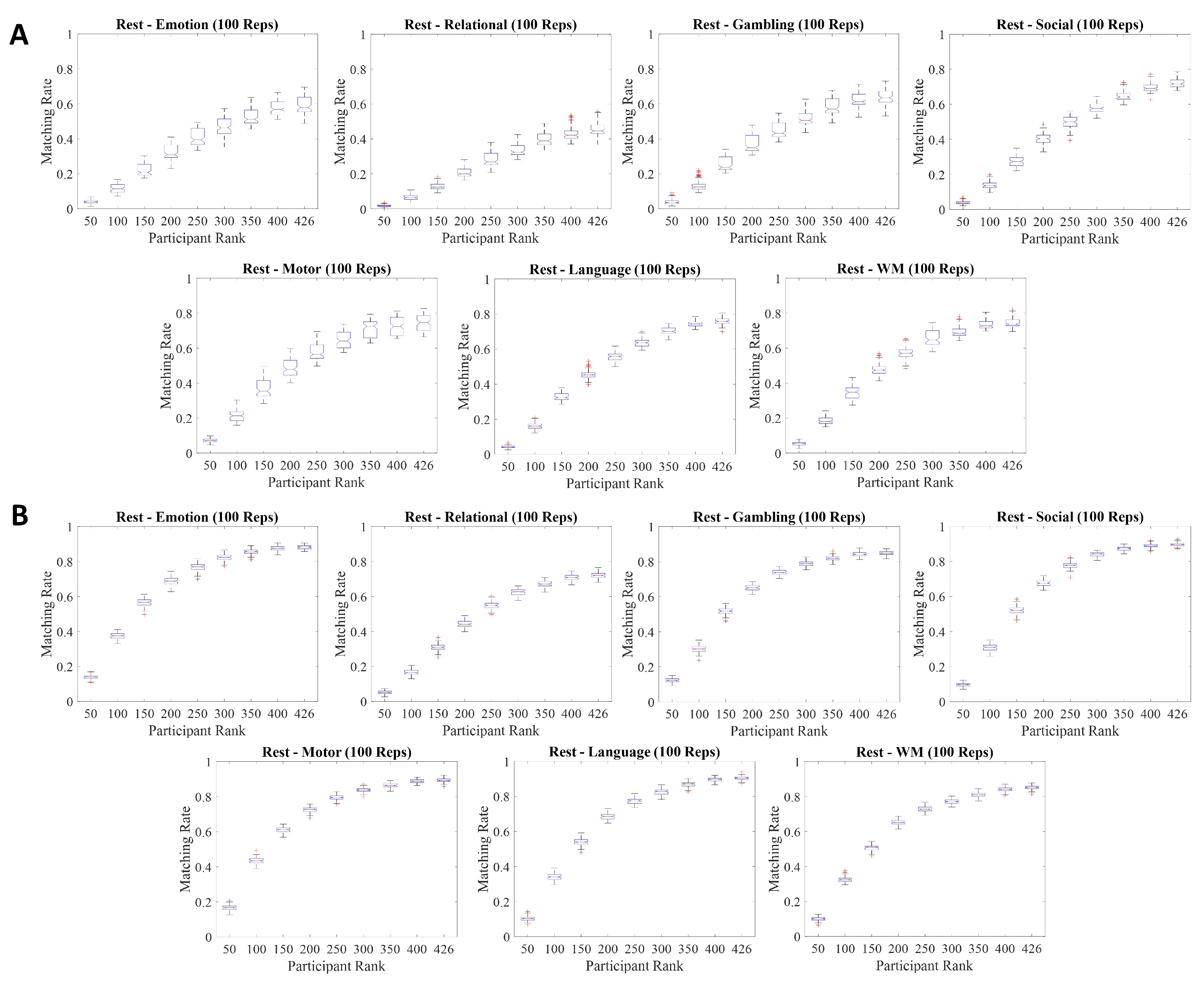
In order to account for scanning length effects, the between-condition matching rate results were obtained when resting-state FCs are estimated by matching the time-series length to each fMRI task. Results are shown in Figure 6. For this analysis, we fixed the brain parcellation rank to 414, which was the optimal choice in terms of fingerprinting as shown in Figure 4. For each participant rank across all between-condition settings, we computed matching rates with 100 different samplings of time points for the resting-state time series. In Figure 6A, we display the results of randomly sampling an initial time point and choosing the remaining time points to be consecutive to it. In Figure 6B, we display the results of randomly sampling all time points. When comparing both sampling strategies, randomly sampling all time points is a more robust and effective approach in terms of fingerprinting, as measured by the standard deviation and mean of each box plot.
4. Discussion
4.1. Brain Parcellation Rank and Participant Rank Effects on Fingerprinting
As shown in Figure 3, compressing the brain parcellation information is detrimental to fingerprinting, as the highest matching rates were obtained with a brain parcellation rank of 414. In contrast, compressing the participants specific dimension overall preserves matching rate, as shown by the high matching rates obtained with participant rank as low as 150 for Relational, Gambling, Social, Language, Working Memory, and Resting-State, and rank of 300 for Emotion and Motor. The results from this analysis imply that the dimension of the participants information, represented by the participants rank, can be considerably compressed into a lower dimensional space while preserving fingerprinting. This indicates that the number of connectivity patterns needed to preserve fingerprinting is significantly smaller than the cohort size. Instead, each individual functional connectome is composed of a unique presence of such functional connectivity patterns. This is because Tucker decomposition decomposes each FC into a weighted sum of underlying functional connectivity patterns, with the weights being the entries in each row vector of the participant factor matrices. It is noteworthy that the percentage of compression found in our results is most likely cohort-size dependent, and hence cannot be extrapolated to other cohort sizes.
4.2. Within-Condition Fingerprinting
The within-condition results shown in Figure 2 validate the existence of a functional connectome fingerprint while showing that a Tucker decomposition based framework is an effective method for uncovering such fingerprints when compared to non decomposed functional connectomes. Notably, our framework yielded substantially higher matching rates than the ones obtained with original FCs for parcellation granularity 214, for which fingerprinting was particularly low (ranging between ). Overall, the matching rate gain brought by Tucker decomposition is higher for lower granularity parcellations.
4.3. Between-Condition Fingerprinting
During resting-state, as opposed to the fMRI tasks, participants are not engaged in any particular stimulus. Hence, with between-condition fingerprinting, we are, in a way, evaluating how similar are the resting-state FCs of participants when compared to their corresponding (engaging) task FCs. To do so, we first learn “default” functional connectivity patterns common to all participants, as represented by the brain parcellation factor matrix derived from the Tucker decomposition of a tensor consisting of resting-state FCs for all participants. Then, when estimating the individual factor matrices for a task fMRI tensor, we identify the underlying resting-state functional connectivity patterns for each participant while engaged in a task. Note that in this case, fingerprinting is more challenging compared to the within-condition setting. Nevertheless, as shown in Figure 5, we were able to significantly increase matching rate relative to using original FCs. Notably, Language is the fMRI condition that showed the smallest fingerprint with the original FC, but the highest by Tucker decomposition.
4.3.1. Times Series Sampling Effects on Between-Condition Fingerprinting
When utilizing the full time series of Resting-State to compute the participants FCs, we obtain promising matching rate results, as highlighted in Figure 5. Interestingly, even though Emotion is the shortest task (166 time-points), between-condition matching rate results are higher than for many of the other (longer) tasks. This might indicate a higher similarity of Emotion FCs to resting-state FCs. For the between-condition analysis, results suggest that matching rates are far more sensitive to changes in the brain parcellation rank as compared to the within-condition setting. This is evident from the significant increase in matching rates observed with a brain parcellation rank of 414 compared to the other ranks.
We also explored the effect of reducing the resting-state scanning length to match the duration of each task. The rationale behind doing so was to determine whether the full scanning length is necessary to extract the “key features” required for obtaining a fingerprint. From both sampling procedures carried out in this study, it is clear that sampling consecutive time points was not an optimal strategy for fingerprinting. Comparing the results of Figure 6A and Figure 6B, we see that randomly sampling time points of resting-state scans is not only more effective than sampling them consecutively, but also as effective as constructing resting-state FCs using the full scan length. This result aligns with the fingerprinting improvements seen when sub-sampling edge time-series frames [41].
4.4. CP vs. Tucker Interpretability on Fingerprinting
Both CP and Tucker decomposition are commonly used tensor decomposition techniques for dimensionality reduction and feature extraction purposes. In the context of fingerprinting, although less computationally expensive, CP falls short due to two key reasons. First, the assumption that the original high-dimensional data can be reconstructed using non-interacting components is too restrictive, as we know that there are innate interactions between brain regions under a functional connectivity standpoint [42]. Second, due to CP decomposition being a single rank decomposition, we cannot freely explore the dynamics of compressing the different dimensions of the data. Conversely, the Tucker’s core plays a pivotal role in capturing the interactions between components while giving us the flexibility to explore how different levels of compression of the brain parcellation and participants information affect fingerprinting, thus overcoming both drawbacks of CP decomposition. However, associating the factor matrices derived from Tucker decomposition to functional connectivity patterns is non-trivial due to the existence of the core tensor [21], which captures several interactions between the components from each factor matrix.
4.5. Limitations and Future Work
Our study has limitations. As mentioned above, there is no trivial way to interpret the factor matrices derived from Tucker decomposition due to the existence of a core tensor that captures the many interactions between all factor matrices [21]. Another limitation of our methodology is that the core and the factor matrices obtained from Tucker decomposition cannot be updated on demand if a new participant FC were to be included in our dataset. Rather, we would have to recompute the Tucker decomposition and perform the entire fingerprinting framework again. To address the interpretability challenges posed by Tucker decomposition, future work could explore ways to make the core tensor sparse while aiming to preserve or maximize FCs fingerprint.
Author Contributions
Conceptualization, V.C, A.M.E.G, J.G; methodology, V.C, M.L., J.H., A.M.E.G, J.G; formal analysis, V.C, A.M.E.G, J.G;; investigation, V.C, M.L., J.H., A.M.E.G, J.G; data curation, V.C, M.L.; writing—original draft preparation, V.C, A.M.E.G, J.G; writing—review and editing, V.C, M.L., J.H., A.M.E.G, J.G; supervision, A.M.E.G, J.G; funding acquisition J.H and J.G. All authors have read and agreed to the published version of the manuscript.
Funding
This research was funded by National Institutes of Health (US), Award ID: CTSI CTR EPAR2169 (J.G). National Institutes of Health (US) R01 AA029607 (J.G), National Institutes of Health (US), Award ID: P60AA07611 (J.H and J.G), National Institutes of Health (US), Award ID: R01NS112303 (J.H and J.G).
Informed Consent Statement
The fMRI dataset used in this study is from the publicly available Human Connectome Project (HCP). Per HCP protocol, written informed consent was obtained from all subjects by the HCP Consortium.
Data Availability Statement
Upon acceptance of this manuscript, Matlab code to perform Tucker Decomposition and subsequent fingerprinting analyses will be available at the CONNplexity Lab website at the Publications section: https://engineering.purdue.edu/ConnplexityLab/publications.
Acknowledgments
Data were provided by the Human Connectome Project, WU-Minn Consortium (Principal Investigators: David Van Essen and Kamil Ugurbil; 1U54MH091657) funded by the 16 NIH Institutes and Centers that support the NIH Blueprint for Neuroscience Research; and by the McDonnell Center for Systems Neuroscience at Washington University.
Conflicts of Interest
The authors declare no conflicts of interest.
Abbreviations
The following abbreviations are used in this manuscript:
| fMRI | Functional Magnetic Resonance Imaging |
| FC | Functional Connectome |
| CP decomposition | CANDECOMP/PARAFAC decomposition |
| HOSVD | Higher Order Singular Value Decomposition |
References
- Behrens, T.E.; Sporns, O. Human connectomics. Current opinion in neurobiology 2012, 22, 144–153. [Google Scholar] [CrossRef] [PubMed]
- Yao, G.; Wei, L.; Jiang, T.; Dong, H.; Baeken, C.; Wu, G.R. Neural mechanisms underlying empathy during alcohol abstinence: evidence from connectome-based predictive modeling. Brain Imaging and Behavior 2022, 16, 2477–2486. [Google Scholar] [CrossRef] [PubMed]
- Fornito, A.; Zalesky, A.; Breakspear, M. The connectomics of brain disorders. Nature Reviews Neuroscience 2015, 16, 159–172. [Google Scholar] [CrossRef]
- Satterthwaite, T.D.; Xia, C.H.; Bassett, D.S. Personalized neuroscience: Common and individual-specific features in functional brain networks. Neuron 2018, 98, 243–245. [Google Scholar] [CrossRef] [PubMed]
- Gratton, C.; Laumann, T.O.; Nielsen, A.N.; Greene, D.J.; Gordon, E.M.; Gilmore, A.W.; Nelson, S.M.; Coalson, R.S.; Snyder, A.Z.; Schlaggar, B.L.; et al. Functional brain networks are dominated by stable group and individual factors, not cognitive or daily variation. Neuron 2018, 98, 439–452. [Google Scholar] [CrossRef]
- Seitzman, B.A.; Gratton, C.; Laumann, T.O.; Gordon, E.M.; Adeyemo, B.; Dworetsky, A.; Kraus, B.T.; Gilmore, A.W.; Berg, J.J.; Ortega, M.; et al. Trait-like variants in human functional brain networks. Proceedings of the National Academy of Sciences 2019, 116, 22851–22861. [Google Scholar] [CrossRef]
- Finn, E.S.; Shen, X.; Scheinost, D.; Rosenberg, M.D.; Huang, J.; Chun, M.M.; Papademetris, X.; Constable, R.T. Functional connectome fingerprinting: identifying individuals using patterns of brain connectivity. Nature neuroscience 2015, 18, 1664–1671. [Google Scholar] [CrossRef]
- Fraschini, M.; Hillebrand, A.; Demuru, M.; Didaci, L.; Marcialis, G.L. An EEG-based biometric system using eigenvector centrality in resting state brain networks. IEEE Signal Processing Letters 2014, 22, 666–670. [Google Scholar] [CrossRef]
- Amico, E.; Goñi, J. The quest for identifiability in human functional connectomes. Scientific reports 2018, 8, 1–14. [Google Scholar] [CrossRef]
- Abbas, K.; Amico, E.; Svaldi, D.O.; Tipnis, U.; Duong-Tran, D.A.; Liu, M.; Rajapandian, M.; Harezlak, J.; Ances, B.M.; Goñi, J. GEFF: Graph embedding for functional fingerprinting. NeuroImage 2020, 221, 117181. [Google Scholar] [CrossRef]
- Cai, B.; Zhang, G.; Hu, W.; Zhang, A.; Zille, P.; Zhang, Y.; Stephen, J.M.; Wilson, T.W.; Calhoun, V.D.; Wang, Y.P. Refined measure of functional connectomes for improved identifiability and prediction. Human brain mapping 2019, 40, 4843–4858. [Google Scholar] [CrossRef] [PubMed]
- Abbas, K.; Liu, M.; Venkatesh, M.; Amico, E.; Kaplan, A.D.; Ventresca, M.; Pessoa, L.; Harezlak, J.; Goñi, J. Geodesic distance on optimally regularized functional connectomes uncovers individual fingerprints. Brain connectivity 2021, 11, 333–348. [Google Scholar] [CrossRef]
- Abbas, K.; Liu, M.; Wang, M.; Duong-Tran, D.; Tipnis, U.; Amico, E.; Kaplan, A.D.; Dzemidzic, M.; Kareken, D.; Ances, B.M.; et al. Tangent functional connectomes uncover more unique phenotypic traits. Iscience 2023, 26. [Google Scholar] [CrossRef]
- Venkatesh, M.; Jaja, J.; Pessoa, L. Comparing functional connectivity matrices: A geometry-aware approach applied to participant identification. NeuroImage 2020, 207, 116398. [Google Scholar] [CrossRef] [PubMed]
- Ng, B.; Dressler, M.; Varoquaux, G.; Poline, J.B.; Greicius, M.; Thirion, B. Transport on Riemannian manifold for functional connectivity-based classification. In Proceedings of the Medical Image Computing and Computer-Assisted Intervention–MICCAI 2014: 17th International Conference, 2014, Proceedings, Part II 17. Boston, MA, USA, 14-18 September 2014; Springer, 2014; pp. 405–412. [Google Scholar]
- Pervaiz, U.; Vidaurre, D.; Woolrich, M.W.; Smith, S.M. Optimising network modelling methods for fMRI. Neuroimage 2020, 211, 116604. [Google Scholar] [CrossRef]
- Dadi, K.; Rahim, M.; Abraham, A.; Chyzhyk, D.; Milham, M.; Thirion, B.; Varoquaux, G.; Initiative, A.D.N.; et al. Benchmarking functional connectome-based predictive models for resting-state fMRI. NeuroImage 2019, 192, 115–134. [Google Scholar] [CrossRef]
- Kolda, T.G.; Bader, B.W. Tensor Decompositions and Applications. SIAM REVIEW 2009, 51, 455–500. [Google Scholar] [CrossRef]
- Mahyari, A.G.; Zoltowski, D.M.; Bernat, E.M.; Aviyente, S. A tensor decomposition-based approach for detecting dynamic network states from EEG. IEEE Transactions on Biomedical Engineering 2016, 64, 225–237. [Google Scholar] [CrossRef] [PubMed]
- Williams, A.H.; Kim, T.H.; Wang, F.; Vyas, S.; Ryu, S.I.; Shenoy, K.V.; Schnitzer, M.; Kolda, T.G.; Ganguli, S. Unsupervised discovery of demixed, low-dimensional neural dynamics across multiple timescales through tensor component analysis. Neuron 2018, 98, 1099–1115. [Google Scholar] [CrossRef]
- Mokhtari, F.; Laurienti, P.J.; Rejeski, W.J.; Ballard, G. Dynamic functional magnetic resonance imaging connectivity tensor decomposition: A new approach to analyze and interpret dynamic brain connectivity. Brain connectivity 2019, 9, 95–112. [Google Scholar] [CrossRef]
- Zhang, Z.; Allen, G.I.; Zhu, H.; Dunson, D. Tensor network factorizations: Relationships between brain structural connectomes and traits. Neuroimage 2019, 197, 330–343. [Google Scholar] [CrossRef] [PubMed]
- Chiêm, B.; Abbas, K.; Amico, E.; Duong-Tran, D.A.; Crevecoeur, F.; Goñi, J. Improving Functional Connectome Fingerprinting with Degree-Normalization. Brain Connectivity 2022, 12, 180–192. [Google Scholar] [CrossRef]
- Tucker, L.R. Some mathematical notes on three-mode factor analysis. Psychometrika 1966, 31, 279–311. [Google Scholar] [CrossRef]
- Van Essen, D.C.; Smith, S.M.; Barch, D.M.; Behrens, T.E.; Yacoub, E.; Ugurbil, K.; Consortium, W.M.H.; et al. The WU-Minn human connectome project: an overview. Neuroimage 2013, 80, 62–79. [Google Scholar] [CrossRef] [PubMed]
- Schaefer, A.; Kong, R.; Gordon, E.M.; Laumann, T.O.; Zuo, X.N.; Holmes, A.J.; Eickhoff, S.B.; Yeo, B.T. Local-global parcellation of the human cerebral cortex from intrinsic functional connectivity MRI. Cerebral cortex 2018, 28, 3095–3114. [Google Scholar] [CrossRef]
- Power, J.D.; Mitra, A.; Laumann, T.O.; Snyder, A.Z.; Schlaggar, B.L.; Petersen, S.E. Methods to detect, characterize, and remove motion artifact in resting state fMRI. Neuroimage 2014, 84, 320–341. [Google Scholar] [CrossRef]
- Glasser, M.F.; Sotiropoulos, S.N.; Wilson, J.A.; Coalson, T.S.; Fischl, B.; Andersson, J.L.; Xu, J.; Jbabdi, S.; Webster, M.; Polimeni, J.R.; et al. The minimal preprocessing pipelines for the Human Connectome Project. Neuroimage 2013, 80, 105–124. [Google Scholar] [CrossRef] [PubMed]
- Smith, S.M.; Beckmann, C.F.; Andersson, J.; Auerbach, E.J.; Bijsterbosch, J.; Douaud, G.; Duff, E.; Feinberg, D.A.; Griffanti, L.; Harms, M.P.; et al. Resting-state fMRI in the human connectome project. Neuroimage 2013, 80, 144–168. [Google Scholar] [CrossRef]
- Amico, E.; Arenas, A.; Goñi, J. Centralized and distributed cognitive task processing in the human connectome. Network Neuroscience 2019, 3, 455–474. [Google Scholar] [CrossRef]
- Cole, M.W.; Bassett, D.S.; Power, J.D.; Braver, T.S.; Petersen, S.E. Intrinsic and task-evoked network architectures of the human brain. Neuron 2014, 83, 238–251. [Google Scholar] [CrossRef]
- Sidiropoulos, N.D.; De Lathauwer, L.; Fu, X.; Huang, K.; Papalexakis, E.E.; Faloutsos, C. Tensor decomposition for signal processing and machine learning. IEEE Transactions on signal processing 2017, 65, 3551–3582. [Google Scholar] [CrossRef]
- Cong, F.; Lin, Q.H.; Kuang, L.D.; Gong, X.F.; Astikainen, P.; Ristaniemi, T. Tensor decomposition of EEG signals: a brief review. Journal of neuroscience methods 2015, 248, 59–69. [Google Scholar] [CrossRef] [PubMed]
- Martınez-Montes, E.; Valdés-Sosa, P.A.; Miwakeichi, F.; Goldman, R.I.; Cohen, M.S. Concurrent EEG/fMRI analysis by multiway partial least squares. NeuroImage 2004, 22, 1023–1034. [Google Scholar] [CrossRef] [PubMed]
- Carroll, J.D.; Chang, J.J. Analysis of individual differences in multidimensional scaling via an N-way generalization of “Eckart-Young” decomposition. Psychometrika 1970, 35, 283–319. [Google Scholar] [CrossRef]
- Harshman, R.A.; et al. Foundations of the PARAFAC procedure: Models and conditions for an" explanatory" multimodal factor analysis 1970.
- Kolda, T.G. Multilinear operators for higher-order decompositions. Technical report, Sandia National Laboratories (SNL), Albuquerque, NM, and Livermore, CA …, 2006.
- Li, X.; Xu, D.; Zhou, H.; Li, L. Tucker tensor regression and neuroimaging analysis. Statistics in Biosciences 2018, 10, 520–545. [Google Scholar] [CrossRef]
- De Lathauwer, L.; De Moor, B.; Vandewalle, J. A multilinear singular value decomposition. SIAM journal on Matrix Analysis and Applications 2000, 21, 1253–1278. [Google Scholar] [CrossRef]
- Penrose, R. A generalized inverse for matrices. In Proceedings of the Mathematical proceedings of the Cambridge philosophical society. Cambridge University Press, Vol. 51; 1955; pp. 406–413. [Google Scholar]
- Cutts, S.A.; Faskowitz, J.; Betzel, R.F.; Sporns, O. Uncovering individual differences in fine-scale dynamics of functional connectivity. Cerebral cortex 2023, 33, 2375–2394. [Google Scholar] [CrossRef]
- Fox, M.D.; Snyder, A.Z.; Vincent, J.L.; Corbetta, M.; Van Essen, D.C.; Raichle, M.E. The human brain is intrinsically organized into dynamic, anticorrelated functional networks. Proceedings of the National Academy of Sciences 2005, 102, 9673–9678. [Google Scholar] [CrossRef]
Figure 1.
Graphic representation of the participant identifiability framework. For an input tensor consisting of FCs from one imaging session, we compute its Tucker decomposition to obtain a core tensor , two identical brain parcellation factor matrices , and a participants’ factor matrix . Fixing and factor matrices, we estimate the participant’s factor matrix for the FCs from another imaging session . We then obtain an identifiability matrix by computing row-wise Pearson’s correlation between and , and obtain a matching rate score through .
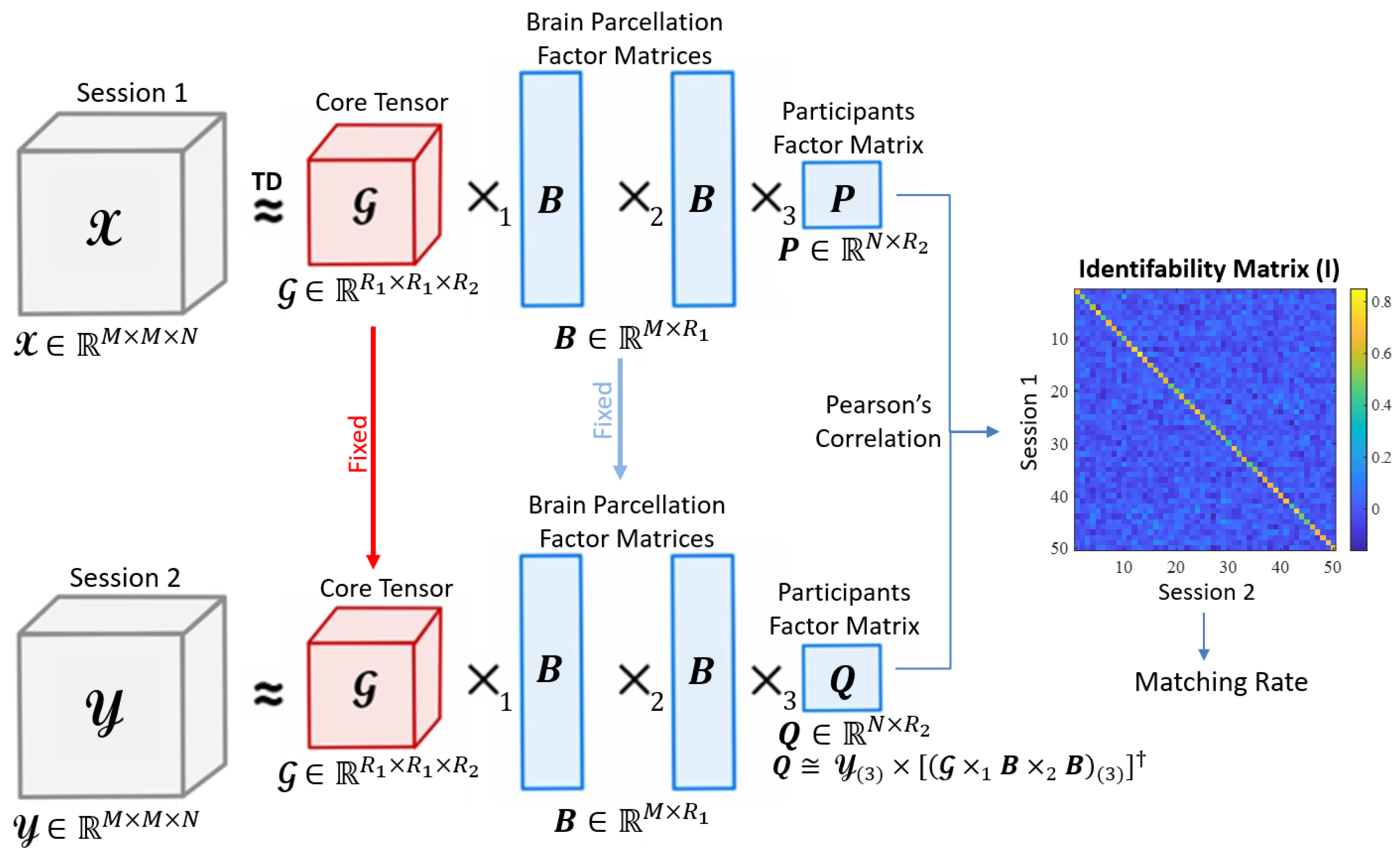
Figure 2.
Within-condition fingerprinting comparisons between highest matching rate obtained with Tucker Decomposition (TD) and with original FCs for all fMRI conditions and parcellation granularities.
Figure 2.
Within-condition fingerprinting comparisons between highest matching rate obtained with Tucker Decomposition (TD) and with original FCs for all fMRI conditions and parcellation granularities.
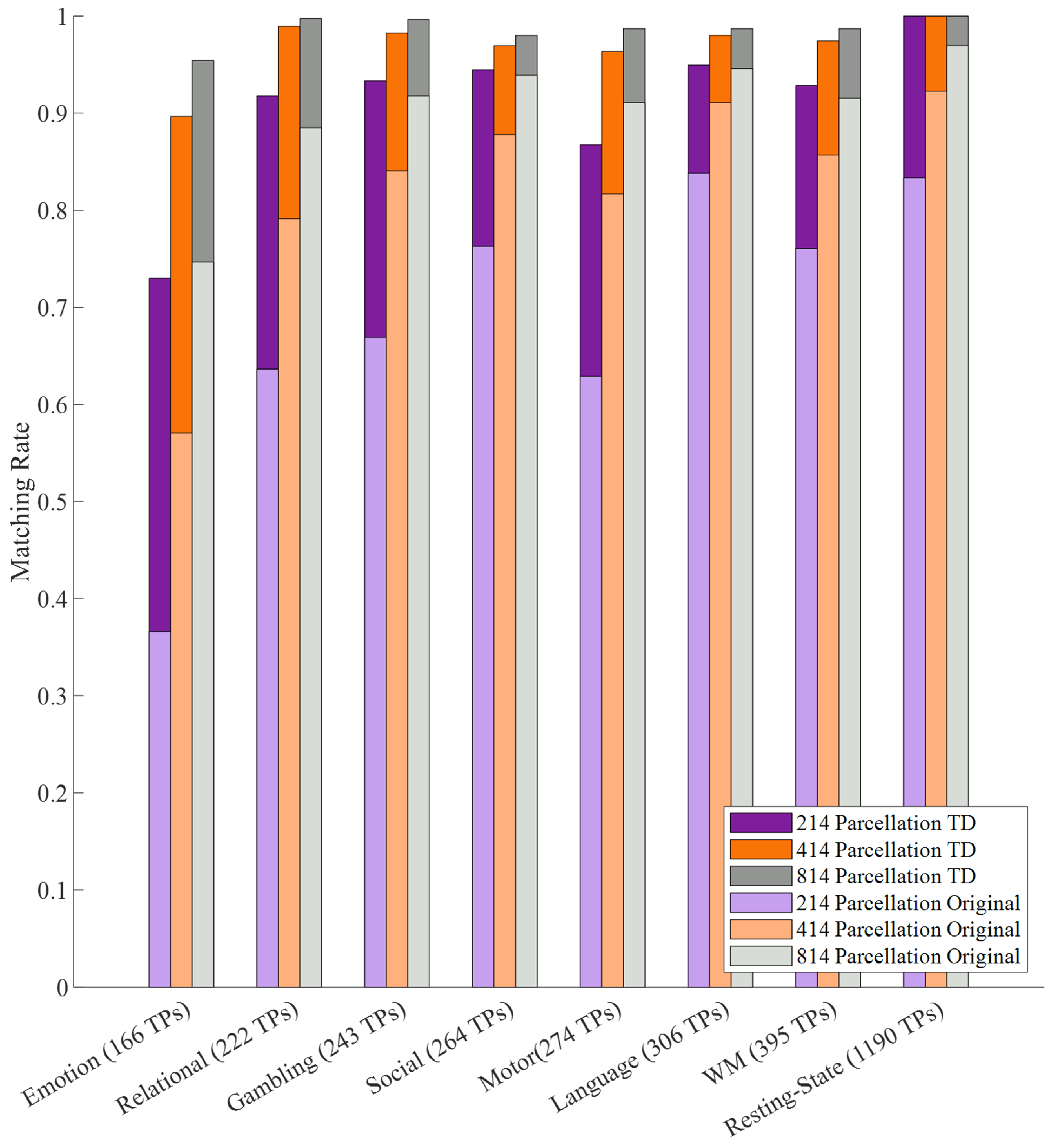
Figure 3.
Brain parcellation rank and participant rank effects on matching rate for all eight fMRI conditions, ordered by scan length (represented by the number of time points “TPs” in their time series) for granularity of Schaefer parcellation 414. For each condition, the fingerprinting framework is applied in both test→retest and retest→test directions. Each curve illustrates the average matching rate computed across both settings at each combination of brain parcellation ranks and participant ranks.
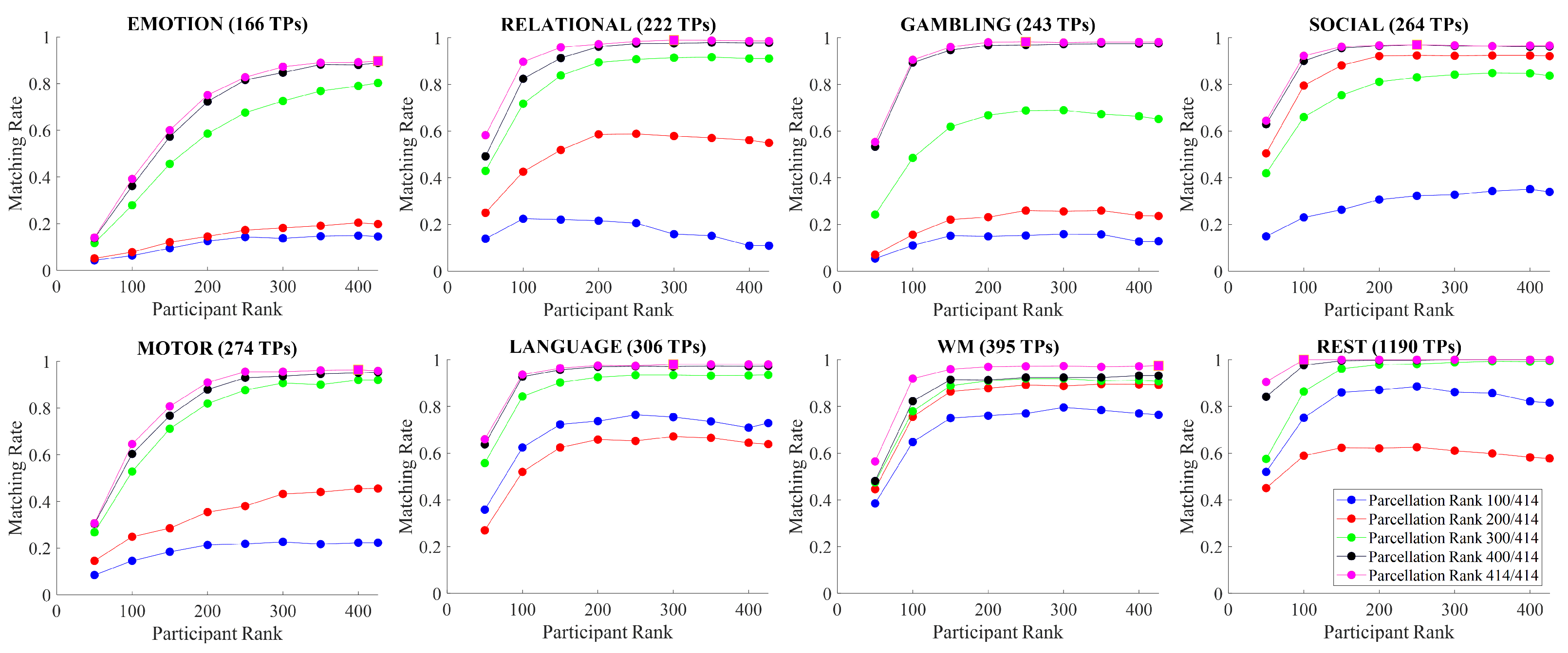
Figure 4.
Brain parcellation rank and participant rank effects on between-condition matching rate for granularity of Schaefer parcellation 414. For each condition, an input tensor of retest resting-state FCs derived from the full scanning length is used to estimate the test task fMRI participant factor matrix.
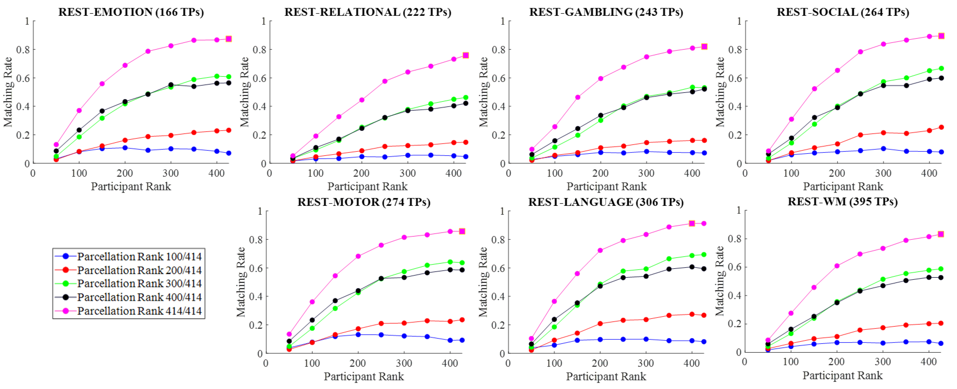
Figure 5.
Comparison between highest between-condition matching rates obtained with our fingerprinting framework based on Tucker Decomposition and original FC matrices for granularity 414.
Figure 5.
Comparison between highest between-condition matching rates obtained with our fingerprinting framework based on Tucker Decomposition and original FC matrices for granularity 414.
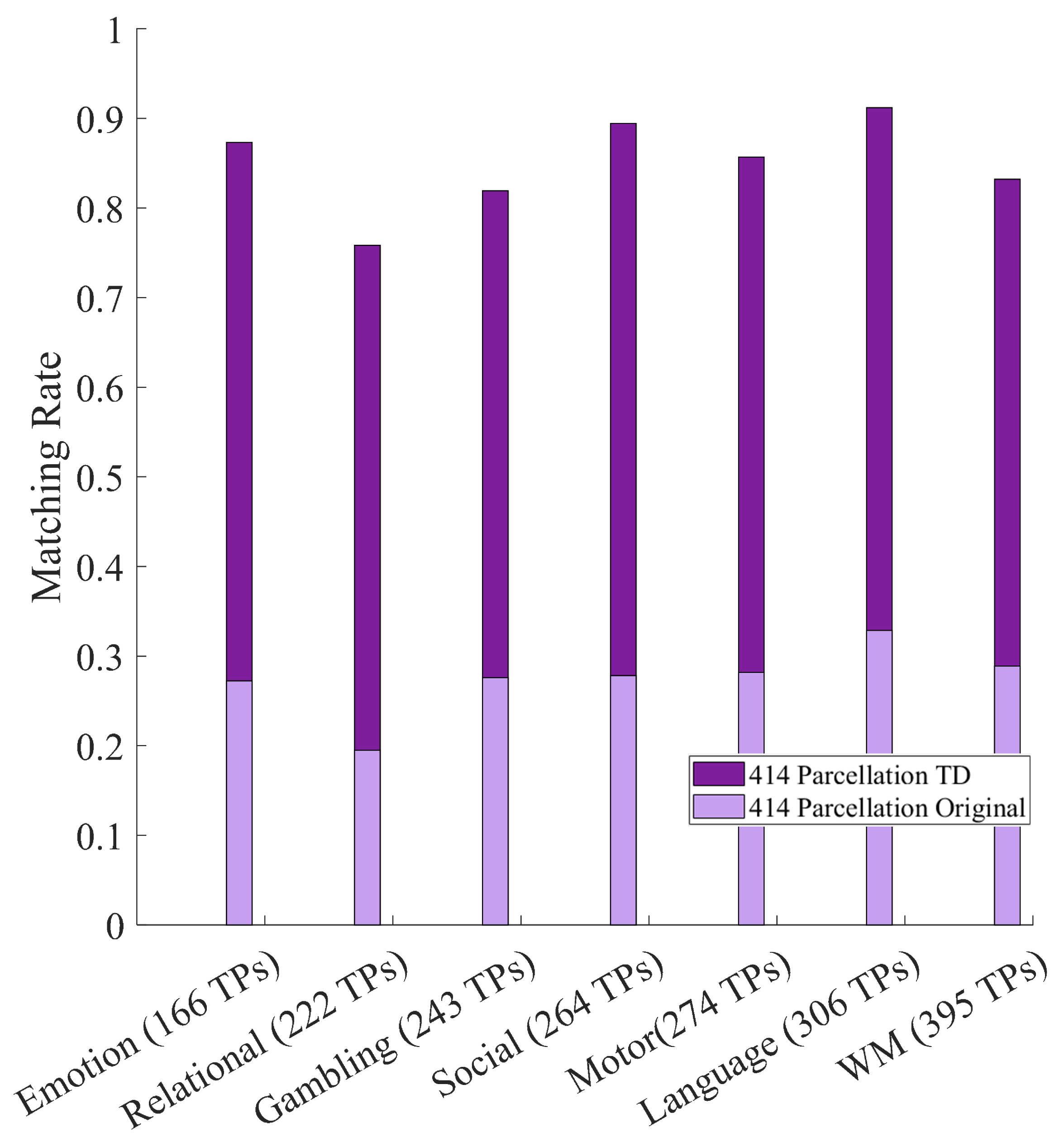
Figure 6.
Matching rate results obtained via Tucker decomposition using reduced time-series to estimate resting-state FCs for the between-condition setting. Results of 100 random sampling trials are shown for parcellation granularity of 414 and brain parcellation rank of 414. A. Rest (retest) - task (test) matching rate results when, starting with a randomly sampled time point, consecutive time points are used to construct resting-state FCs. B. Matching rates when randomly sampled time points are used to construct resting-state FCs.
Disclaimer/Publisher’s Note: The statements, opinions and data contained in all publications are solely those of the individual author(s) and contributor(s) and not of MDPI and/or the editor(s). MDPI and/or the editor(s) disclaim responsibility for any injury to people or property resulting from any ideas, methods, instructions or products referred to in the content. |
© 2025 by the authors. Licensee MDPI, Basel, Switzerland. This article is an open access article distributed under the terms and conditions of the Creative Commons Attribution (CC BY) license (http://creativecommons.org/licenses/by/4.0/).
Copyright: This open access article is published under a Creative Commons CC BY 4.0 license, which permit the free download, distribution, and reuse, provided that the author and preprint are cited in any reuse.


