
Submitted:
12 February 2025
Posted:
12 February 2025
You are already at the latest version
Abstract
Travel time information has become an essential component of everyday commuting. Without such information, schedule delays would increase, leading to inevitable losses in traveler utility. In Korea, dedicated short-range communication transponders that identify vehicles have been installed along signalized arterials to collect travel time data. By matching vehicle identifications at consecutive points, travel times can be measured. However, for travel time information to be effective, two types of data processing techniques are required: outlier filtering and travel time prediction. This study proposes algorithms to address both challenges. An outlier filtering algorithm based on the median-based confidence interval was developed, taking into account the travel time characteristics on suburban arterials with frequent entry and exit points. Additionally, a travel time prediction algorithm that integrates Long Short-Term Memory (LSTM) and Convolutional Neural Network (CNN), referred to as LSTM-CNN, was developed to capture both long-term trends and local patterns in travel time data. The implementation of these algorithms resulted in a 2.2% reduction in error rates under congested conditions compared to current practices. At the 4-kilometer study site, the annual benefits from this error reduction could amount to $135,200.
Keywords:
Travel time
; DSRC
; Outlier filtering
; Prediction
; CNN
; LSTM
1. Introduction
Travel time information has become an essential
aspect of daily life. Without access to such information, social utility may
diminish due to early or late arrivals, leading to wasted time that could
otherwise be allocated to more valuable activities. To collect travel time
data, two types of traffic detectors have been deployed: point detectors and
section detectors. Point detectors measure vehicle speed at a specific
location, and travel time is estimated by dividing the distance by the measured
speed. Section detectors, on the other hand, identify vehicles at distinct
locations and match vehicle identifications at two consecutive points to
calculate travel time. Point detectors have been recognized as effective for
uninterrupted facilities, but they present limitations on interrupted
facilities due to delays at intersections. Consequently, section detectors,
which can directly measure travel times, have been installed on signalized
arterials. As of 2021, 270 dedicated short-range communication (DSRC) transponders
that identify passing vehicles were deployed on suburban arterials in Korea [1]. However, travel time information in DSRC
systems on signalized arterials faces two main challenges: outlying travel time
data and time lags in collected data.
Outlying observations primarily occur due to exit
and re-entry maneuvers between section detectors. Signalized arterials
typically feature frequent intersections and roadside businesses along the
route, which can lead to frequent exit and re-entry maneuvers. If these
outlying observations are not properly addressed, the travel time information
may become unreliable. Moreover, as travel time data are collected when
vehicles complete their trips within section detector systems, the recorded
travel times inherently exhibit a time lag. This lag renders the information
less useful for drivers who are beginning their trips along the route. To
address the issue of outliers, an outlier filtering algorithm needs to be
developed, and to mitigate the time lag, a prediction technique must be
applied. Currently, a median filter and k-Nearest Neighbor (k-NN) techniques
are employed in the DSRC system. However, the median filter alone is
insufficient for identifying all valid travel times, and the k-NN algorithm has
demonstrated limitations in predicting travel times under congested conditions.
Therefore, further improvements are necessary to enhance the effectiveness of
the DSRC-based traffic information system.
In this study, two key challenges were addressed.
To resolve the outlier issue, a median-based confidence interval concept was
derived. To mitigate the time-lag phenomenon, a deep learning model combining
Long Short-Term Memory (LSTM) and Convolutional Neural Networks (CNN) was
proposed. The proposed techniques were compared to the current methods, which
rely on a simple median filter for outlier filtering and k-Nearest Neighbor
(k-NN) for travel time prediction. Finally, the superiority of the developed techniques
over the existing practices was thoroughly discussed.
2. Previous Research
2.1. Outlier Filtering
Numerous studies have been conducted to filter
outlying travel times from valid data sets. In the early stages, outliers were
removed using a mean-based threshold approach, where valid travel times in
subsequent aggregation intervals were defined within a specific range based on
the mean travel time of the previous interval [2–4].
However, this simple threshold scheme did not accurately capture the full range
of travel time patterns, leading to the exclusion of valid travel times when
the threshold was too low, and the inclusion of outliers when the threshold was
too high. To address the limitations of the mean-based threshold, more complex
algorithms were proposed [5–7]. However, these
sophisticated algorithms have shown limitations regarding real-time
application, and the need to estimate multiple parameters has hindered their
practical use in real-world systems.
The DSRC system examined in this study currently
employs a median filter, where the average travel time is estimated using the
median value within each aggregation interval. The median filter has
demonstrated advantages in terms of practicality and reliability over
conventional algorithms; however, it is still unable to identify all valid
travel times. To analyze travel time patterns or distributions in greater
detail, it is essential to obtain all valid individual travel times. Therefore,
there is a need to develop a robust outlier filtering algorithm that not only
identifies each valid travel time but also ensures practical applicability.
2.2. Travel Time Prediction
In the early stages, several techniques—including
the Kalman filter, nonparametric time series analysis models, regression
analysis, and k-NN models—were employed to forecast travel times for real-time
traveler information [8–11]. Among these, k-NN
models were found to be particularly effective for travel time prediction up
until the mid-2010s [12–17]. However, the need
for k-NN models to identify the k-nearest neighbors each time new data is
received posed a significant challenge for real-time applications.
Additionally, the computational resources required to operate the k-NN
algorithm were substantial compared to other models.
In the late 2010s, deep learning models garnered
significant attention in the field of travel time forecasting. Numerous
pioneering studies investigated the application of LSTM and
sequence-to-sequence (seq2seq) models, revealing that their performance substantially
outperforms that of conventional models [18–26].
However, these studies primarily utilized individual deep learning models,
suggesting that the integration of composite models could further enhance
predictive accuracy.
The DSRC system examined in this study employs a
k-NN model for travel time prediction. Acknowledging the limitations of k-NN
models and the emergence of more advanced deep learning techniques, the
operators of the DSRC system have been exploring artificial intelligence models
to enhance the reliability of travel time predictions. In this context, an
innovative deep learning model that integrates two architectures (CNN and LSTM)
has been developed.
3. Methodology
3.1. Outlier Filtering
As discussed earlier, to address the current issues
with outlier treatment—ensuring both practicality and the inclusion of all
valid travel times—a robust outlier filtering algorithm (Equations 1–4) based
on the concept of confidence intervals was proposed. In determining the
confidence interval, the median, rather than the mean, was utilized and
adjusted with correction factors to account for the travel time data’s tendency
to deviate abnormally from the valid values (refer to Figure 4(a)). This filtering algorithm
effectively identifies all valid data points that fall within the established
confidence interval.
where:
- ·
- = average of valid travel times from A to B at time t,
- ·
- = number of samples in 5-min block of travel times,
- ·
- = set of valid travel times from A to B at time t,
- ·
- = aggregation (collection) interval,
- ·
- = detection time of vehicle i (or m) at point A (or B), and
- ·
- 1.253 and 1.35 = conversion factors (refer to [27–29] ).
The developed filtering algorithm is practically
applicable to real-world systems, as it does not require the estimation of
complex parameters used in previous studies. Typically, the aggregation
interval is set at 5 minutes. During each five-minute interval, the median and
standard error (SE) of all travel times recorded by traversing vehicles are
calculated, and a confidence interval (e.g., 95%, 99%) is derived based on
these values. Finally, individual travel times falling within this confidence
interval are identified as valid data.
3.2. Travel Time Prediction
As previously described, various deep learning
models have been employed to forecast travel times. However, most prior studies
have predominantly utilized a single model. In this study, a hybrid model was
proposed to effectively capture both long-term and local patterns in travel
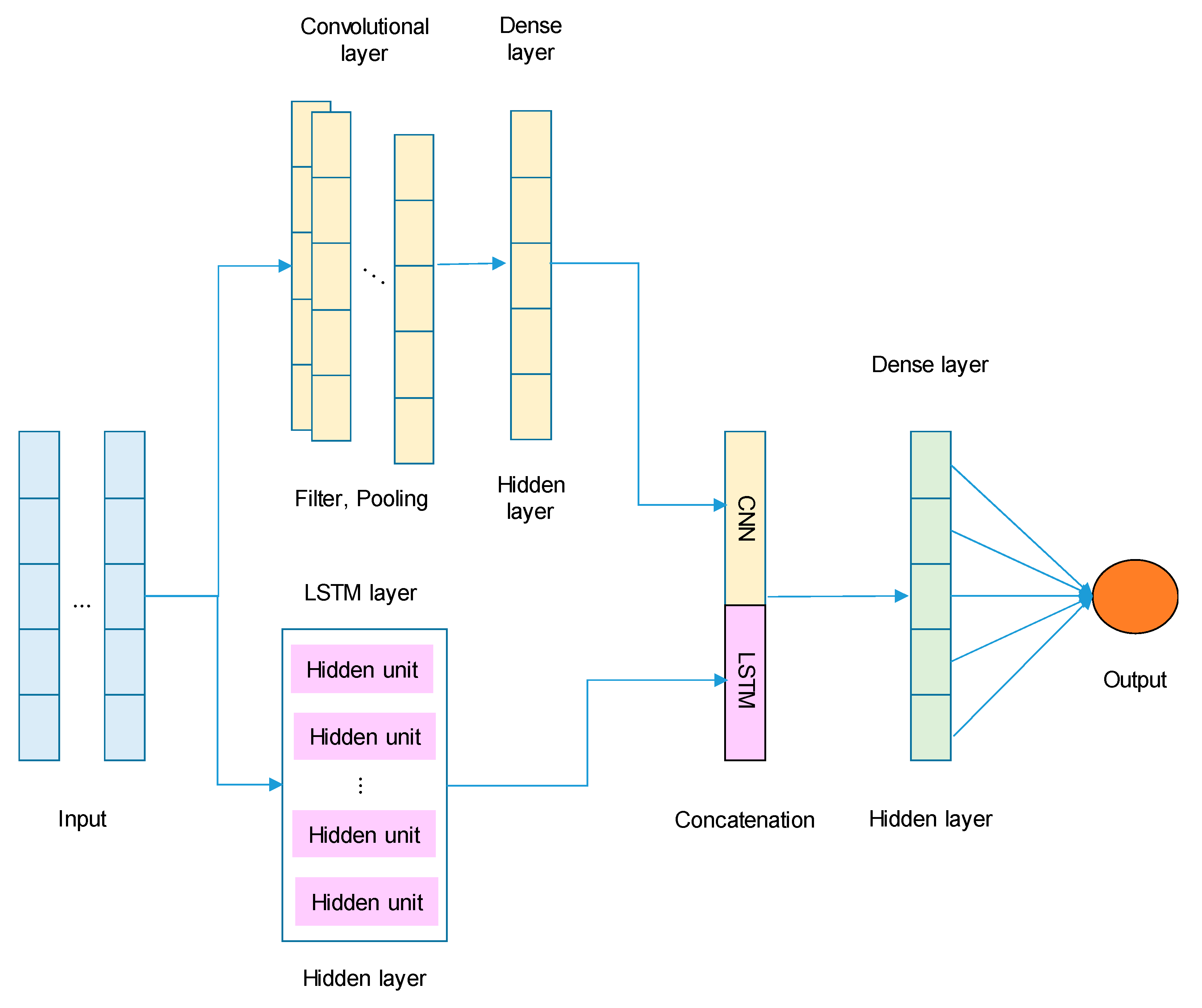
time data, thereby enhancing prediction accuracy. The proposed Long Short-Term
Memory-Convolutional Neural Network (LSTM-CNN) model integrates an LSTM network
(equations 5-10) with CNNs (equation 11). This architecture is designed to
capture temporal dependencies through LSTMs and spatial or local patterns
through CNNs in the time-series travel time data. The architecture of the
LSTM-CNN model is depicted in Figure 1.
Both components operate independently to learn temporal and local patterns,
respectively, followed by a concatenation layer to integrate their outputs.
In an LSTM network, the key equations govern the
behavior of the gates (forget, input, and output) and the cell state. The LSTM
equations are as follows:
where:
- ·
- = input at time step t,
- ·
- = hidden state from the previous time step,
- ·
- and = previous and present cell states,
- ·
- = forget, input, and output gates,
- ·
- = candidate cell state,
- ·
- = input weights for gates and cell state,
- ·
- = recurrent weights,
- ·
- = biases,
- ·
- and = sigmoid and hyperbolic tangent function, and
- ·
- = element-wise multiplication.
Figure 1.
LSTM-CNN Architecture.
In a CNN, the convolution operation is fundamental.
The convolution process can be represented by the following equation:
where:
- ·
- = output feature map at position , and channel ,
- ·
- = input value at position for channel ,
- ·
- = convolution filter weights,
- ·
- = bias term for channel , and
- ·
- and = dimensions of the filter and kernel.
The benefits of the proposed LSTM-CNN model over
the previous models that exclusively utilized a single model are as follows:
- Temporal and spatial dependencies: LSTM effectively captures long-term temporal dependencies, while CNN extracts spatial or local patterns from the data.
- Multi-scale learning: CNN captures patterns at multiple scales through convolutional filters, aiding in the detection of important features in time-series data.
- Dimensionality reduction: Pooling layers in CNN reduce dimensionality and computational complexity, thereby enhancing model efficiency.
4. Study Site
To evaluate the developed algorithms, travel time
data were collected from a DSRC-based traffic information system deployed on
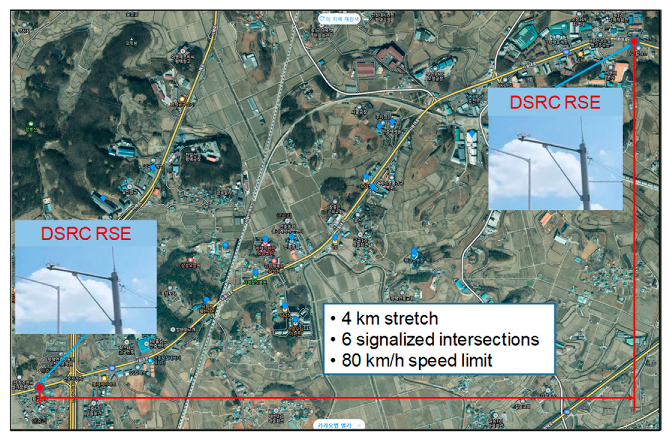
National Highway 38 in Pyeongtaek region of South Korea. As illustrated in Figure 2, the study section spans 4 km and
comprises a total of six signalized intersections. DSRC Roadside Equipment
(RSE) was installed at both ends of the section to record the passing times of
vehicles equipped with DSRC On-Board Unit (OBU). As of the time the
experimental data were collected, approximately 60% of vehicles in Korea were
equipped with DSRC OBUs.
Despite the posted speed limit of 80 km/h, the
average speed during non-congested periods was around 50–60 km/h due to the
high density of traffic signals along the route. The area is situated near an
industrial complex, leading to congestion during weekday morning commutes.
Since there is no congestion on weekends due to the lack of commuter traffic,
data collection focused on weekdays in January 2013, when morning congestion
was consistently observed.
Figure 2.
Experiment segment.
The baseline data for the evaluation were generated
by the operators of the DSRC system. These operators manually identified valid
travel times based on their prior knowledge of the section and monitoring
results from surveillance cameras installed along the route. The baseline data
verified by the operators are depicted in Figure
3, and the descriptive statistics are presented in Table 1.
Figure 3.
Baseline travel times (5-minute aggregation interval mean).
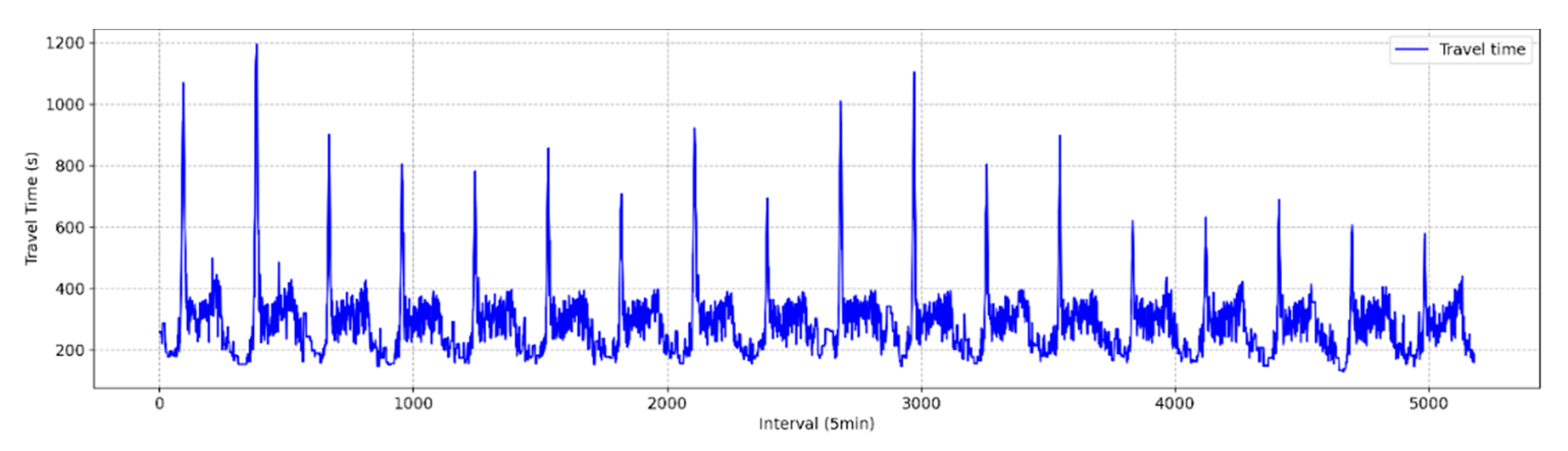
The travel time data were aggregated at 5-minute
intervals, in alignment with the DSRC-based traffic information system deployed
on the National Highway. Daily congestion was observed between 8:00 and 9:00
AM, whereas in the afternoon, although traffic volume increased, the rise in
travel time was less pronounced compared to the morning peak period. A total of
5,181 data points were collected at 5-minute intervals over approximately 18
days. As indicated in Table 1, the
average travel time for the study section was 286 seconds, with a standard
deviation of 106 seconds, a minimum of 130 seconds, and a maximum of 1,193
seconds. The maximum travel time was nearly five times the average,
highlighting significant congestion during morning peak hours.

Table 1.
Descriptive statistics of travel time.
| Statistic | Travel time (s) |
| Count Mean Standard deviation Minimum Maximum |
5,181 286 106 130 1,193 |
5. Generation of Travel Time Information
5.1. Outlier Filtering
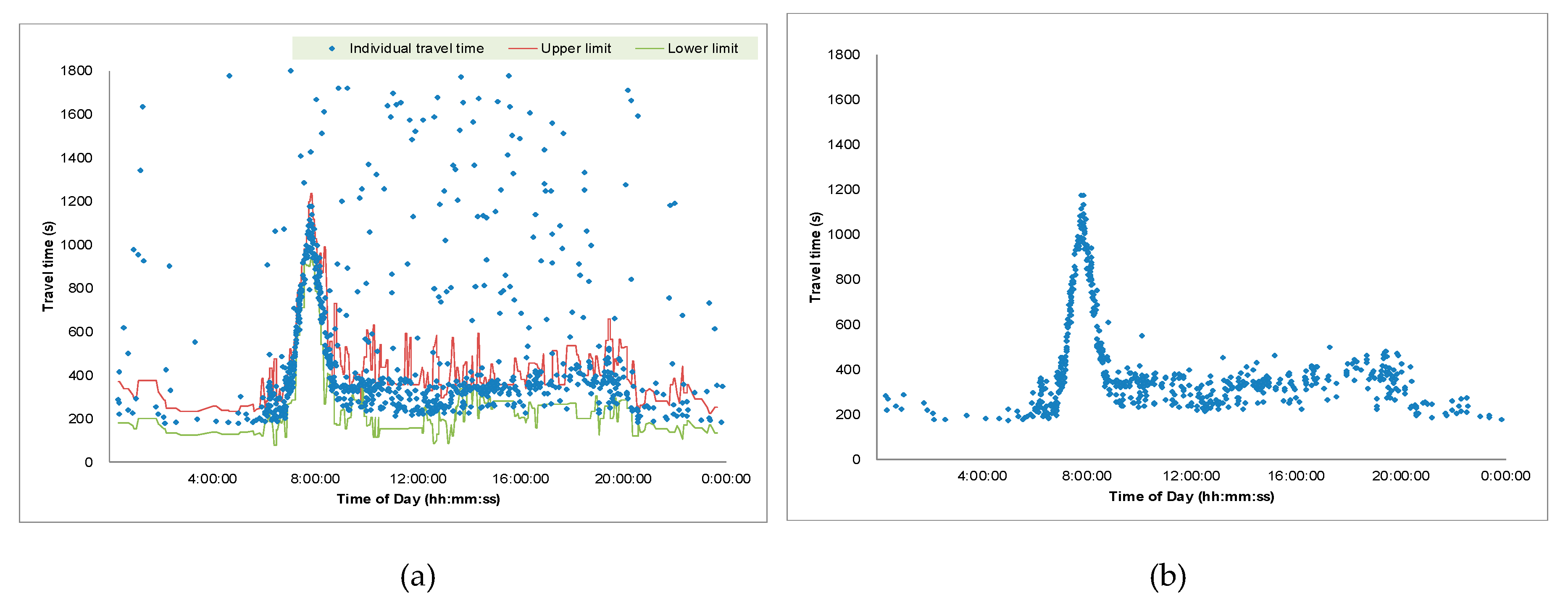
The proposed outlier filtering algorithm was
applied to the collected weekday travel time data described previously. A
one-day example is illustrated in Figure 4,
demonstrating that all apparent outliers were successfully filtered after
applying the algorithm. As mentioned earlier, the current practice generates
only one median value per aggregation interval (5 minutes), which prevents the
identification of individual travel time records. In contrast, when the
developed algorithm is applied, all individual travel time records can be
retrieved, as shown in Figure 4(b).
The algorithm's capability to capture the entire
set of valid travel times allows practitioners to gain deeper insights into
travel time patterns. For example, it reveals that the variability of travel
times under congested conditions is relatively small compared to that under
uncongested conditions. This is likely attributable to the nature of
interrupted flow facilities, where travel times tend to vary more widely under
free-flow conditions due to traffic signal effects. In contrast, during
congestion, the influence of signals diminishes as vehicles queue. Leveraging
this understanding, operators could refine travel time information
dissemination strategies, such as providing a range of travel times instead of
a single average value. Additionally, by obtaining individual travel times,
valuable traffic statistics—such as travel time reliability and various
descriptive measures—can be derived, which are otherwise unattainable using the
current practice.
Figure 4.
Individual travel time: (a) raw data, (b) outlier-filtered data.
5.2. Travel Time Prediction
The proposed LSTM-CNN algorithm was implemented
using the TensorFlow Keras framework. The filtered travel time data were
standardized using the MinMaxScaler to improve prediction performance. A
target prediction interval of 30 minutes was selected. No significant
differences in performance were observed when varying the prediction target
from 10 minutes to one hour. Consequently, the feature columns included travel
times at both the current time and 30 minutes ahead, while the label column
represented the travel time at 30 minutes ahead. The window size for time
series analysis was set to 288 (5 minutes * 288 = 24 hours) to capture the
recurrent daily travel time pattern. The processed data were then split into a
7:3 ratio for training and testing.
The grid search technique was employed to identify the optimal parameters. Table 2 presents the parameters explored and the corresponding optimal values determined for each model. To prevent overfitting, the EarlyStopping function with a patience of five was applied, restoring the best weights where the mean square error was minimized. Additionally, a dropout rate of 0.3 was applied to the final dense layer. The training process, as depicted in Figure 5, shows that the reduction in error became relatively small after four epochs.
6. Evaluation
The forecasted travel times were evaluated using three widely-recognized metrics (Equations 12-14): Mean Absolute Error (MAE), Root Mean Square Error (RMSE), and Mean Absolute Percentage Error (MAPE). MAE, the mean of absolute errors, is intuitively easier to interpret compared to RMSE. However, RMSE assigns greater weight to larger errors than MAE, often resulting in higher values. According to a study [30], MAE is more appropriate when errors follow a normal distribution, whereas RMSE is better suited for errors following a Laplace distribution. Therefore, both measures are typically employed to assess prediction performance. MAPE converts MAE into a percentage, facilitating comparison across different scales and improving interpretability.
where:
- ·
- = observed value,
- ·
- = predicted value, and
- ·
- = number of sample.
The predicted travel times generated by the current and proposed techniques were evaluated using the baseline data described in Figure 3. Table 3 presents the results for the three metrics: MAE, RMSE, and MAPE. The performance of the proposed methodology demonstrated a slight improvement (1.3%) over the current practice. Although the improvement was modest, it was found to be statistically significant, as determined by a paired t-test at a significance level of 0.05 (see Table 4). Figure 6 and Figure 7 depict the comparisons between actual and predicted travel times for the current and proposed algorithms. Given the heightened emphasis on travel time information under congested conditions, the prediction performances were categorized into congested and non-congested conditions, with a threshold of 300 seconds (1.5 times the free-flow travel time of 200 seconds). The results indicated the performance improvement (2.2%) of the proposed method was more pronounced under congested conditions, as shown in Table 5 and Figure 8.
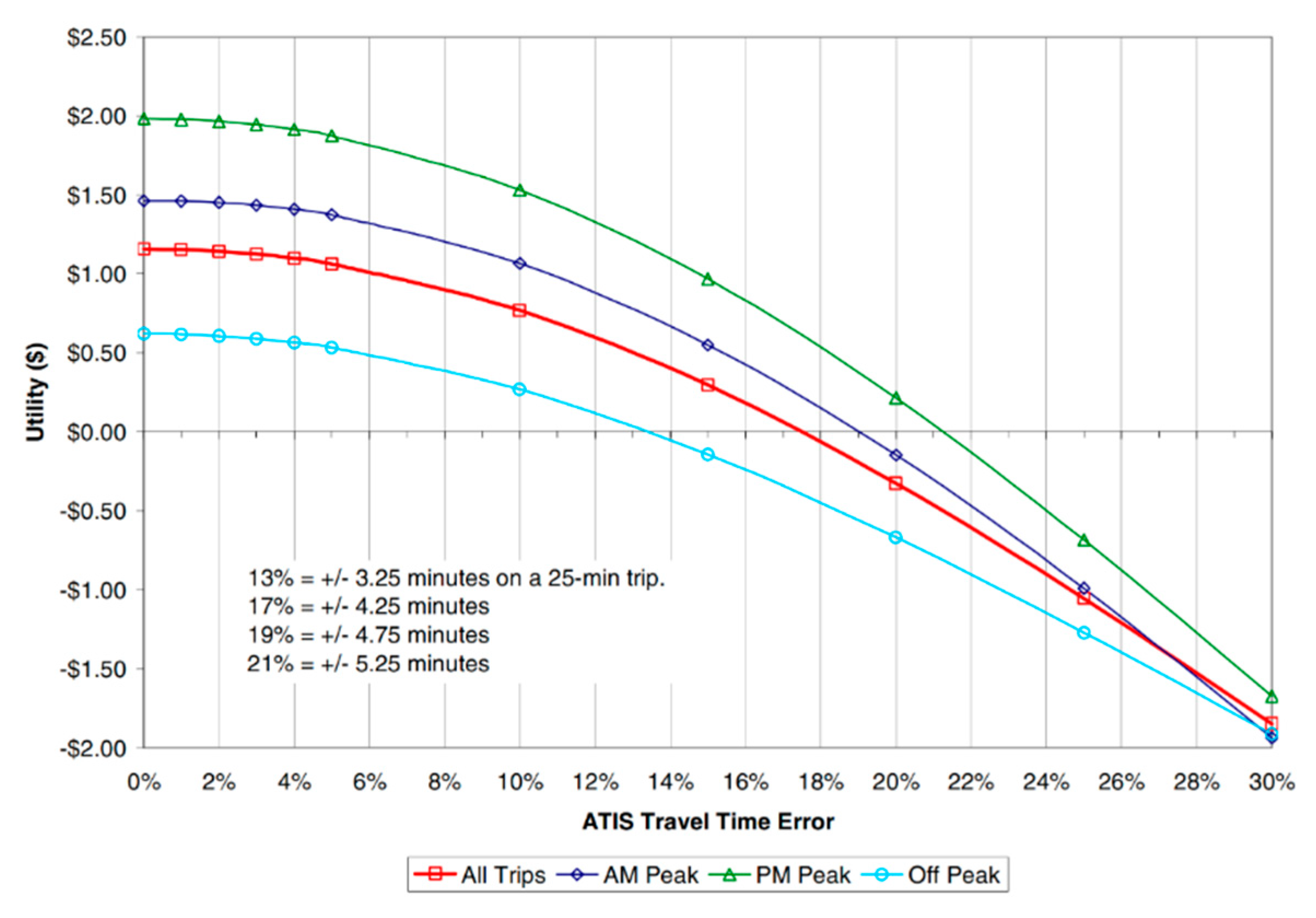
Estimating the improvement in prediction performance in monetary terms could provide valuable insights. For this purpose, the travel time information utility function developed by Toppen was employed. The underlying logic of the utility function, based on data collected in Los Angeles, is that reduced schedule delays result from more accurate travel time information. Schedule delays occur when travelers arrive either earlier or later than expected due to inaccurate travel time information. This suggests that reliable travel time information increases traveler utility by enabling them to use their time more productively. Figure 9 presents the traveler utility curve developed by Toppen [31]. According to the graph, a 2.2% reduction in error during the morning peak corresponds to a utility increase of $0.20 per person. When applied to the average traffic volume and passenger occupancy on the 4 km stretch of the study site, this could translate to an approximate annual social benefit of $135,200.
- $ 0.20 * 2,000 vehicles * 1.3 passengers * 5 days * 52 weeks = $ 135,200
Figure 9.
Traveler utility as a function of travel time error (source: A. Toppen, 2004).
8. Conclusions and Future Studies
Real-time travel time information is a critical element in our daily life. Despite numerous studies conducted over the past several decades, drivers continue to demand more reliable travel time data. To address this need, advanced data processing techniques for DSRC-based traffic information systems have been developed. Prior to this development, current practices and previous studies were thoroughly reviewed, with their limitations identified. These findings underscore the necessity for further advancement in algorithms for outlier filtering and travel time forecasting.
The developed outlier filtering algorithm is grounded in the concept of a median-based confidence interval. Appropriate statistical modifications were applied to the median to utilize the confidence interval of the normal distribution. The proposed technique was implemented on raw travel time data collected from a signalized arterial and demonstrated its effectiveness in censoring outliers from valid travel times. In contrast to the current practice, where a single median value is extracted for every 5-minute aggregation interval, the developed algorithm retrieves the entire set of valid data. This advancement allows operators to acquire more detailed insights into travel time patterns, enhancing travel time information provision strategies and statistical analyses.
To address the time-lag effect in DSRC-based traffic information systems, a hybrid model combining LSTM and CNN architectures, referred to as the LSTM-CNN model, was proposed. This deep learning model demonstrated superior performance, achieving a 2.2% reduction in error compared to the traditional k-NN algorithm when applied to outlier-filtered travel time data. Unlike previous studies that employed only a single deep learning model, the proposed hybrid model captures both long-term and local patterns simultaneously. Furthermore, the performance improvement was quantified in monetary terms, yielding an estimated annual social benefit of $135,200 on the 4-km experimental stretch.
While the developed algorithms have been rigorously tested on the experimental section characterized by recurrent congestion, further application to travel time data from diverse arterial roads is necessary to ensure their generalizability. Additionally, more advanced deep learning models could be employed to achieve further error reduction, ultimately enhancing traveler utility.
Acknowledgments
This paper was supported by a research project (No. 20240190-001) from the Korea Institute of Civil Engineering and Building Technology, funded by the Ministry of Science and ICT.
References
- Ministry of Land, Infrastructure, and Transport (2021), ITS Basic Plan 2030 (Plan to Provide Smart Transportation Services Based on Multi-layered Communications and Cooperation Between Facilities and Modes).
- Southwest Research Institute: Automatic vehicle identification model deployment initiative-system design document. Texas Department of Transportation. 1998.
- S D Clark, Grant-Muller S, Chen H: Cleaning of matched license plate data. Transportation Research Record: Journal of the Transportation Research Board. 2002.
- Francois D, Hesham R: Estimating dynamic roadway travel times using automatic vehicle identification data for low sampling rates. Transportation Research Part B. 2006. [CrossRef]
- Ma X, Koutsopoulos H: Estimation of the automatic vehicle identification based spatial travel time information collected in Stockholm. IET Intelligent Transport Systems. 2010. [CrossRef]
- Dan V B, William H S IV, Casey B: Innovative real-time methodology for detecting travel time outliers on interstate highways and urban arterials. Transportation Research Record: Journal of the Transportation Research Board. 2011.
- Jinhwan J: Data-cleaning technique for reliable real-life travel time estimation: use of dedicated short-range communications probes on rural highways. Transportation Research Record: Journal of the Transportation Research Board. 2016. [CrossRef]
- Jinhwan J: Short-term travel time prediction using the Kalman filter combined with a variable aggregation interval scheme. Journal of the Eastern Asia Society for Transportation Studies. 2013.
- H. Kim and K. Jang (2013), “Short-Term Prediction of Travel Time Using DSRC on Highway”, Journal of the Korean Society of Civil Engineers, Vol. 33, No. 6. pp. 2455-2471. [CrossRef]
- W Qiao, A Haghani, M Mamedi. A nonparametric model for short-term travel time prediction using Bluetooth data. Journal of Intelligent Transportation Systems, 17(2): 165-175, Taylor and Francis Group, 2013. [CrossRef]
- W Qiao, A Haghani, C Shao, J Liu. Freeway path travel time prediction based on heterogeneous traffic data through nonparametric model. Journal of Intelligent Transportation Systems, Vol. 20, No. 5, Taylor and Francis Group, 2013.
- J Myung, D Kim, S Kho, C Park. Travel time prediction using k nearest neighbor method with combined data from vehicle detector system and automatic toll collection system. Transportation Research Record: Journal of the Transportation Research Board, Volume 2256, 2011. [CrossRef]
- S Wu, Z Yang, X Zhu, B Yu. Improved k-NN for short-term traffic forecasting using temporal and spatial information. Journal of Transportation Engineering, 140(7), American Society of Civil Engineers, 2014. [CrossRef]
- S Lim, H Lee, S Park, T Heo. A study of travel time prediction using k-nearest neighborhood method. The Korean Journal of Applied Statistics, 26(5): 835, 2013 (in Korean). [CrossRef]
- S Tak, S Kim, K Jang, H Yeo. Real-time travel time prediction using multi-level k-nearest neighbor algorithm and data fusion method. In: Computing in Civil and Building Engineering, American Society of Civil Engineers, Orlando, Florida, 2014.
- B Yu, X Song, F Guan, Z Yang, B Yao. k-nearest neighbor model for multi-time-step prediction of short-term traffic condition. Journal of Transportation Engineering, 142(6), 2016.
- J Zhong, S Ling. Key factors of k-nearest neighbor nonparametric regression in short-time traffic flow forecasting. In: Proceedings of the 21st International Conference on Industrial Engineering and Engineering Management 2014, Atlantis Press, 2015.
- S. Lim, H. Lee, S. Park, and T. Heo (2013), “A Study of Travel Time Prediction using k-Nearest Neighborhood Method”, Applied Statistics Research, 26(5), pp. 835-845. [CrossRef]
- D. Han, J. Kim, and S. Kim (2018), “Evaluation of Travel Time Prediction Reliability on Highway Using DSRC Data”, Journal of Intelligent Transport Systems, 17(4), pp. 86-98. [CrossRef]
- K. Jang, S. Jo, Y. Jo, and S. Son (2020), “Development of Fire Engine Travel Time Estimation Model for Securing Golden Time”, Journal of Intelligent Transport Systems, 19(6), pp. 1-13.
- J. Lee, S. Son, and H. Kim (2019), “Long-term Prediction of Freeway Travel Time Using Route Travel Data”, Journal of Korean Society of Transportation, Vol.37, No.5, pp.399-409. [CrossRef]
- J. Park and C. Roh (2023), “The Development of Travel Time Forecast Methodology using Individual Vehicle Speed of Dedicated Short-Range Communication (DSRC)”, Journal of the Korea Academia-Industrial Cooperation Society, Vol. 24, No. 11 pp. 893-899. [CrossRef]
- Y. Duan, Y. L.V., and F Wang (2016), “Travel time prediction with LSTM neural network”, 2016 IEEE 19th International Conference on Intelligent Transportation Systems (ITSC), Rio de Janeiro, Brazil, 2016, pp. 1053-1058.
- N.C. Petersen, F. Rodrigues, and F.C. Pereira (2019), “Multi-output bus travel time prediction with convolutional LSTM neural network”, Expert Systems with Applications, Volume 120, pp. 426-435. [CrossRef]
- N. Zhang, F. Wang, X. Chen, T. Zhao, and Q. Kang (2022), “Spatial-temporal attention-based seq2seq framework for short-term travel time prediction”, International Journal of Bio-Inspired Computation, Vol. 20. No. 1, pp. 23-37. [CrossRef]
- M. Ho, Y. Chen, C. Hung, and H. Wu (2021), “A Hybrid Deep Learning Network for Long-Term Travel Time Prediction in Freeways”, 2021 International Conference on Technologies and Applications of Artificial Intelligence (TAAI), Taichung, Taiwan, pp. 78-83.
- Y. Liu, H. Zhang, J. Jia, B. Shi, and W. Wang (2023), “Understanding urban bus travel time: Statistical analysis and a deep learning prediction”, International Journal of Modern Physics B, Vol. 37, No. 04. [CrossRef]
- P. Roy, R. Laprise, and P. Gachon (2016). Sampling Errors of Quantile Estimations from Finite Samples of Data, arXiv:1610.03458.
- X. Wan, W. Wang, J. Liu, and T. Tong (2014), Estimating the Sample Mean and Standard Deviation from the Sample Size, Median, Range and/or Interquartile Range, BMC Medical Research Methodology 14 (135). [CrossRef]
- M. Bland (2015), Estimating Mean and Standard Deviation from the Sample Size, Three Quartiles, Minimum, and Maximum, International Journal of Statistics in Medical Research, Vol. 4, pp. 57-64. [CrossRef]
- T. O. Hodson (2022), Root-mean-square error (RMSE) or mean absolute error (MAE): when to use them or not, Geoscientific Model Development, Vol. 15, pp. 5481–5487. [CrossRef]
- Toppen, S. Jung, V. Shah, and K. Wunderlich (2004). Toward a Strategy for Cost-Effective Deployment of Advanced Traveler Information Systems, Transportation Research Record, 1899(1), pp. 27-34. [CrossRef]
Figure 5.
Learning process of LSTM-CNN.
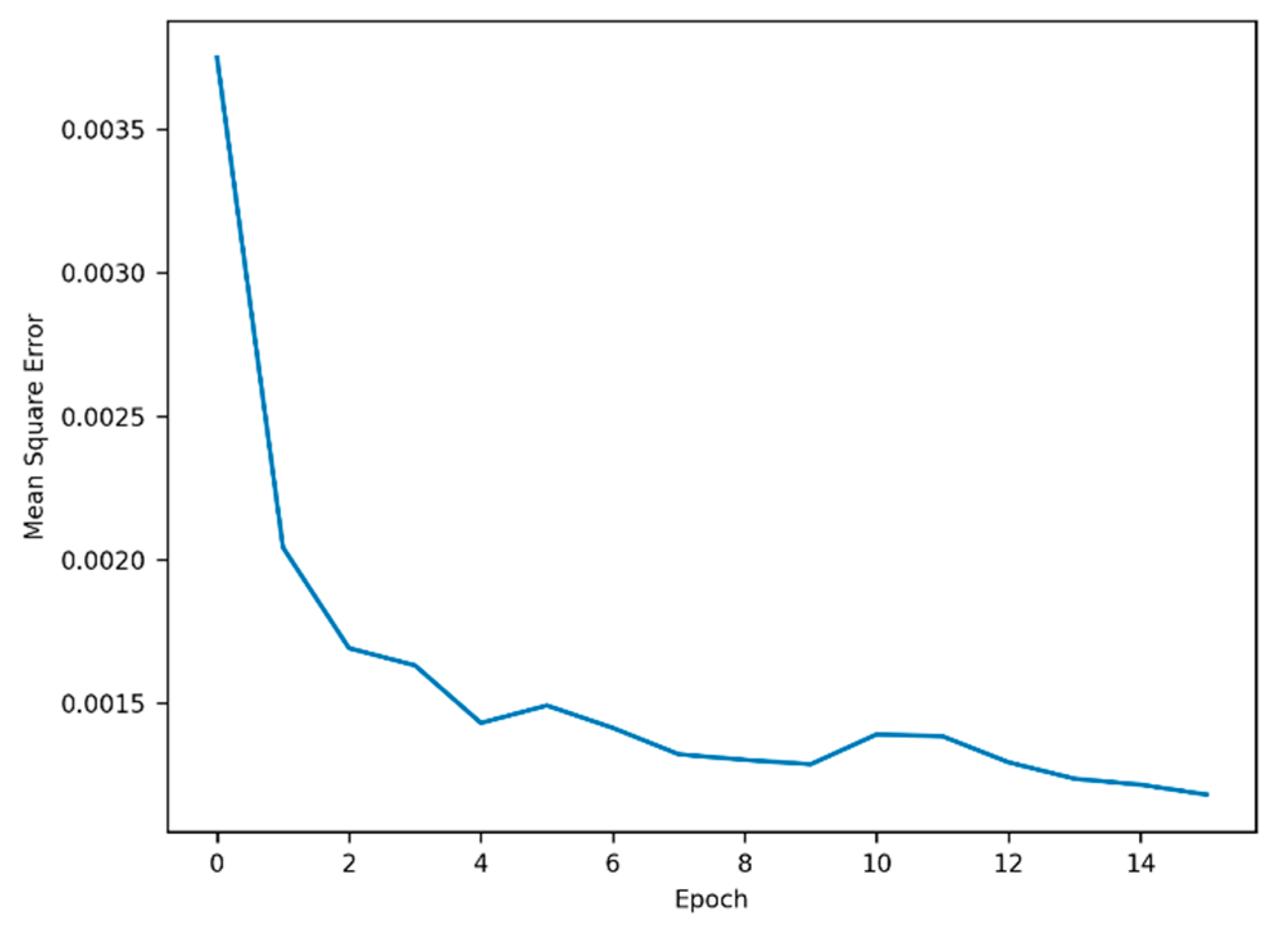
Figure 6.
Comparison of predicted travel time and actual travel time (Current).
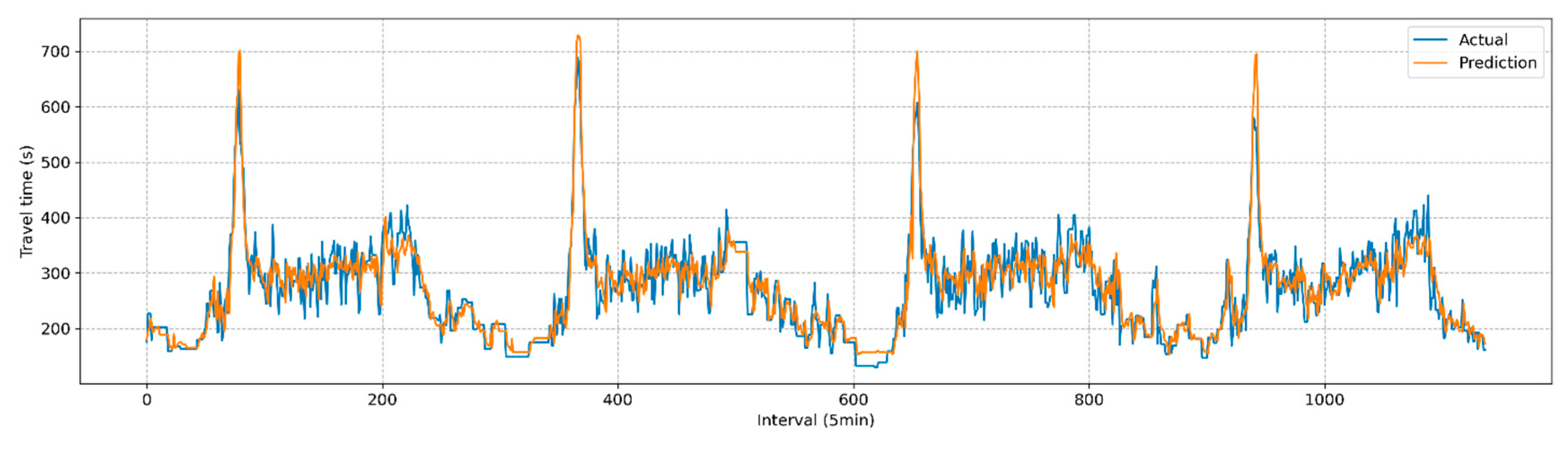
Figure 7.
Comparison of predicted travel time and actual travel time (Proposed).
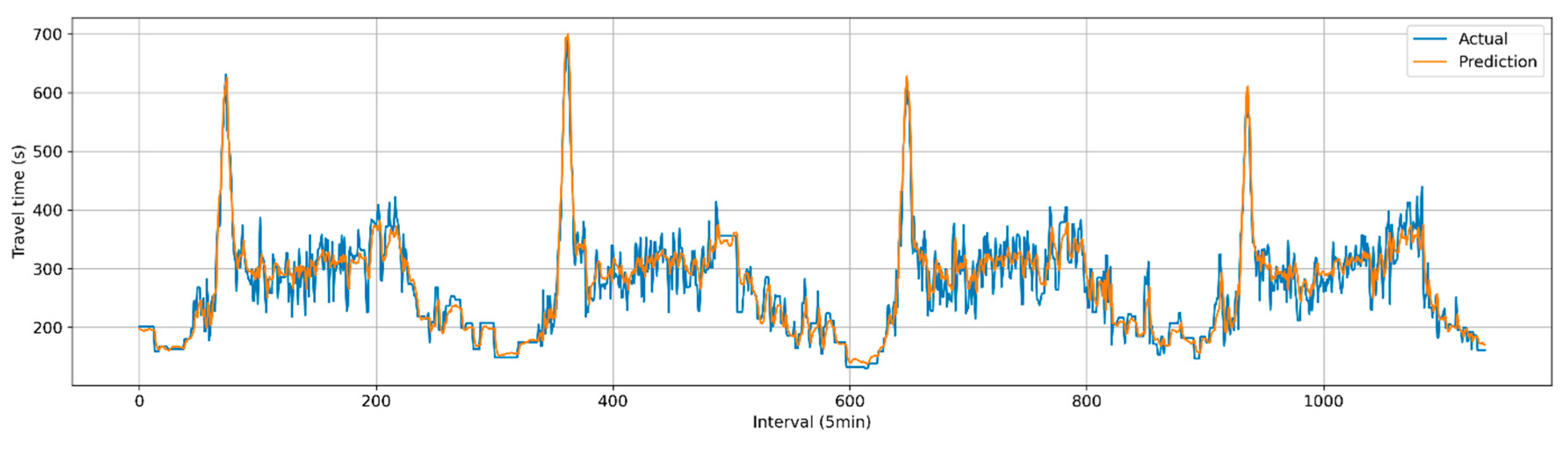
Figure 8.
Travel time error differences between models by flow conditions.

Table 2.
LSTM-CNN parameters.
| Model | Parameter | Search grid | Optimal parameter |
| LSTM | Number of hidden node Activation function Window size |
[64, 128, 256] [Sigmoid, Tanh] [144, 288, 576] |
128 Tanh (hyperbolic tangent) 288 (24 hours) |
| CNN | Number of layer Activation function |
[1, 2, 3] [Sigmoid, ReLU] |
2 ReLU |
Table 3.
Travel time error.
| Measure | Currenta | Proposed b |
| MAE (s) RMSE (s) MAPE (%) |
27.3 37.3 10.3 |
23.9 32.3 9.0 |
a median + k-NN; b proposed outlier filtering algorithm + LSTM-CNN.
Table 4.
Paired t-test of MAPE.
| Statistic | Currenta | Proposed b |
| Mean Variance Number of sample t-statistic t-statistic at sig. lev. of 0.05 p-value (one-sided) |
10.3 83.6 1,137 3.52 1.65 0.0002 |
9.0 70.3 |
Table 5.
Paired t-test of MAPEs by flow conditions.
| Statistic | Travel time > 300 s | Travel time ≤ 300 s | ||
| Current | Proposed | Current | Proposed | |
| Mean Variance Number of sample t-statistic t-statistic at sig. lev. of 0.05 p-value (one-sided) |
10.8 99.6 388 4.62 1.65 2.27e-6 |
8.6 65.7 |
9.8 76.7 749 0.93 1.65 0.18 |
9.3 51.9 |
Disclaimer/Publisher’s Note: The statements, opinions and data contained in all publications are solely those of the individual author(s) and contributor(s) and not of MDPI and/or the editor(s). MDPI and/or the editor(s) disclaim responsibility for any injury to people or property resulting from any ideas, methods, instructions or products referred to in the content. |
© 2025 by the authors. Licensee MDPI, Basel, Switzerland. This article is an open access article distributed under the terms and conditions of the Creative Commons Attribution (CC BY) license (http://creativecommons.org/licenses/by/4.0/).
Copyright: This open access article is published under a Creative Commons CC BY 4.0 license, which permit the free download, distribution, and reuse, provided that the author and preprint are cited in any reuse.


