Submitted:
11 February 2025
Posted:
12 February 2025
You are already at the latest version
Abstract
The mesoscopic phase separation in two- and three-dimensional gels has been studied by computer simulation of a bead-spring model of Lennard-Jones particles. The formation of complex networks of high density phase (HDP) has been investigated and partially explained with competing short- and long-range energies. HDP network formation was found to occur at certain combinations of temperature and spring coefficient, given sufficient particle density. The morphology of the HDP networks changed with these three parameters. HDP networks became more faceted with higher spring coefficients, wider but less dense at higher temperatures and more voluminous and compact at larger densities. HDP network formation was preceded by a stage of HDP precipitation and followed by a stage of surface minimization.
Keywords:
networks
; gels
; simulation
; molecular dynamics
; Lennard-Jones particles
; bead-spring model
; phase separation
; high density phase
; morphology
; surface optimization
1. Introduction
Polymer networks, so-called gels, can undergo two types of phase transitions: volume transitions and phase separation. This study focuses on phase separation, where the gel separates into regions with high and low polymer concentrations. Up to now, research on phase separation in gels has mainly treated surface effects [1,2]. Thus the processes occurring within the bulk of the gel are a welcome object of study for simulations, as we still lack proper methods of physical investigation [1,2]. Comprehensive understanding and prediction of micro phase separation in gels could be of great use for applications where the gel’s microstructure plays a role. Two examples are the development of iongel soft solid electrolytes for solid-state batteries [3,4,5] and the comprehension of the complex deformation behavior exhibited by gels [6].
Motivated by earlier studies [7], which indicated phase separation with a characteristic length scale significantly larger than a model grid size, Peleg et al. [1,2] introduced a simplistic model to mimic the collection of long and short range forces in a gel. The model consists of particles (representing polymer density) interacting via a Lennard-Jones (LJ) potential (short range attraction typifying polymer crystallization) connected through harmonic springs (entropy elasticity) in a two-dimensional simple square lattice structure. Their simulations revealed that, under certain circumstances, the gel phase separates into a high density phase (HDP) and a low density phase (LDP) with the HDP forming a filamentous, foam-like network.
This paper strives to offer further insight into the structure and formation of those HDP networks and to take a step further by generalizing Peleg et al.’s [1,2] model to three dimensions. Of particular interest were the parameters allowing the formation of such structures, their process of formation and their morphology.
2. Materials and Methods
2.1. Model
In the two-dimensional elastic LJ toy model proposed and investigated by Peleg et al. [1,2,8] the gel is represented by particles initially arranged in a two-dimensional square (or hexagonal) lattice. Using LJ units, each particle is attributed a mass of one and is connected permanently to its four initially neighboring particles through weightless harmonic springs. These springs have a spring coefficient, denoted as K, and an equilibrium length of zero. Additionally, pairwise interactions between particles occur via a short range 12-6-LJ potential, which is truncated beyond a cutoff radius .
By employing periodic boundary conditions (PBC), the network of harmonic springs functions as long-range repulsive forces, causing the particles to move apart, to their simple cubic lattice positions. Conversely, the LJ forces operate at close range, attempting to "glue" the particles together. For three dimensions this model was expanded to a simple cubic lattice (Figure 1a). Here, each particle is connected permanently to its six initially neighboring particles. The dimension dependent quantities such as distance and temperature were adapted accordingly.
2.2. Molecular Dynamics
The three-dimensional model was studied by a molecular dynamics (MD) simulation in the canonical ensemble. LJ-units are used throughout, i.e., physical units were kept dimensionless. The system was initialized as a simple cubic lattice of N particles and the volume of the simulation box was set to give the desired number density . At startup, each particle was attributed a pseudo-random velocity vector according to a Maxwell-Boltzmann (MB) distribution with specific kinetic energy , while the overall momentum was constrained to be zero. Newton’s equations of motion were integrated by a Velocity Verlet algorithm with an integration time step . Temperature was kept constant by periodic velocity rescaling, applied every hundredth time step.
2.3. Force Calculations
The springs were set up in a way, that permanently connected a particle to the nearest periodic-boundary-condition copy of its four/six initial neighbors. In all simulations, spring lengths stayed well below one half of the simulation box length, ensuring consistency. For d dimensions only springs had to be checked for the spring force calculations. Thus they used only a small part of the total computing time.
The main bottleneck of these large MD simulations were the calculations of the LJ forces. With more than hundred thousand particles and therefore (potentially) several billion LJ force calculations per time step it became imperative to optimize this process. This was achieved by the implementation of neighbor lists. This effectively reduced the number of LJ force calculations per time step by grouping the particles into neighborhoods. The neighborhood of a given particle was made to consist of all other particles, which were likely to interact with it until the next update of the neighbors lists. In the present work, the neighborhood of a particle encompassed all other particles closer than an estimated radius:
where denotes the cutoff radius, the number of time steps between neighbor list updates, the time step, and T the temperature.
These neighbor lists are most effective at low temperatures facing an even particle distribution at low density. At larger temperatures, the neighborhood radius (1) increases and hence the neighborhoods encompass more particles, which reduce their effectiveness. An uneven particle distribution has a similar effect, increasing the particle count of neighbor lists of all HDP particles drastically. It was chosen to update the list every hundredth time-step . We checked that the criterion (1) ensures that all interactions are properly taken into account for all systems studied (see Appendix A).
As programming language and framework MATLAB was used. All two-dimensional simulations were run and analyzed on a desktop PC (Intel i7-6700 CPU), the three-dimensional simulations were run on the ETH-Zurich Euler cluster. Attempts at using LAMMPS [9] to simulate this model were unsuccessful.
2.4. Methods of Investigation
The evolving HDP networks were of a complex nature. Several methods have been found to describe the gels structure: (i) graphical representation, (ii) minimal particle distribution (MPD), (iii) spring length distribution (SLD), and (iv) radial shell density distribution (RSD).
(i) Figure 1b and c show a graphical representation of the trajectories of the simulated gel. The connecting springs were drawn with a limited number of points per line. This had the effect of rendering extended springs transparent and contracted springs opaque. In two dimensions, springs smaller than were colored orange highlighting the HDP. In three dimensions, foam-like structures consisting of faces and filaments evolved. To increase the visibility of these structures, each spring was colored according to its spacial orientation. Over all this had the effect of highlighting faces and coloring them according to their orientation.
(ii) To determine the MPD of a gel state, for each particle the distance to its closest neighbor was measured. Then a binning algorithm was applied, with thousand equally spaced binning intervals ranging from zero to one fifth of the simulation box length.
(iii) To construct the SLD, this same binning algorithm was used on all current spring lengths instead of the minimal radial particle distances.
(iv) The RSD, which is the radial distribution function not normalized by the bulk density, is usually calculated by measuring all pairwise particle distances, then adding, binning and normalizing them. With a gel of particles this would have meant calculating and binning distances. To keep the calculation effort reasonable, for each particle one percent of the other particles were chosen at random to then measure the distances. The binning was carried out with 2500 binning intervals over half of the simulation box length and therefore with the same binning interval length, or more precisely the same thickness of the spherical binning shell as for the MPD and SLD. The resulting distribution was then normalized by the volume of the binning shell () and by the number of sample distances per particle ().
To monitor the evolution of the structure over time, several measures were taken to express the gels structure in one number per time frame. This process is sketched in Figure 2. Any two particles closer to each other than a critical distance of were declared HDP particles (see Figure 2). The simulation box was then regularly separated into small cubes of edge length . To cancel out random agglomerates, such a small cube needed to encase more than four HDP particles to be declared full. Thereafter a new grid of big cubes with edge length was created - each big cube therefore consisting of eight small cubes in three dimensions or four in two dimensions. A big cube was now declared to be a surface cube, if at least one, but not all of its small cubes were full. The above values for agglomerate threshold, the size of a small box, the number of small cubes making up a big cube and the upper and lower limit for a big cube to be a surface cube were adjusted graphically to fit the HDP structures visible by eye as good as possible.
By this algorithm the following three numbers were obtained: the number of HDP particles , the number of full (small) cubes , and the number of (big) surface cubes . From these, five quantities of interest could be obtained for two and three dimensions d: namely the relative HDP surface area
the fraction of HDP particles (only the particles inside of the small cubes were counted)
the HDP volume fraction
the density of the HDP
and lastly the thickness of the HDP filaments
This Eq. (6) approximates the filament as an infinitely long cylinder, where the total surface is dominated by the curved surface area. There the ratio of volume to surface is
for the radius r. This is the ratio used in Eq. (6) to get a rough measure of thickness.
The same argument can be made in two dimensions, taking a rectangle instead of a cylinder.
In addition to these structural measures, the total static energy of the system was calculated as the sum of the total pairwise LJ energy
and the total spring energy
Here denotes the scalar distance between particles i and j, and symbolizes a spring connection between them.
3. Results
3.1. Evolution of a HDP Network
Under certain conditions, the gel could be observed to phase separate into a complex network of HDP, enclosing regions of LDP. Figure 3 shows this at the example of a two- and a three-dimensional gel. In both examples, small HDP precipitates could be seen from the start. Over time they grew and connected to each other to form a complex HDP network.
To monitor this evolution, the three-dimensional gel’s trajectories were analyzed according to the measures established in Section 2.4. Figure 4a shows particle fraction , volume fraction and density of the HDP. All three measures showed a rapid increase at the beginning which slowed down over time until asymptotic behavior was prevalent. The final volume occupied by the HDP was little less than concentrating off all particles to a density of inside the HDP.
The evolution of the relative HDP surface area is shown in Figure 4b. Two stages can be observed. First, as HDP precipitated and precipitates grew larger than the agglomerate threshold, the relative HDP surface area increased. Later, after reaching a maximum of (HDP surface area was larger than one side area of the surface cube) between and , the relative HDP surface area decreased again, until transitioning to asymptotic behavior towards end of the simulation. Relative HDP surface area and HDP volume fraction are linked over Eq. (6) to give the HDP filament thickness . This HDP filament thickness decreased to a minimum just until the onset of HDP network formation visible by eye (see Figure 3) and then increase to an asymptotic value of (simulation box length was about ).
The evolution of the gels static energies showed a decrease in total LJ energy with a lesser increase in total spring energy leading to a decrease in total static energy over the course of the simulation (see Figure 4c). After an erratic first phase, the changes in all energies slowed down to become asymptotic towards the end of the simulation.
To further analyze the morphology of the evolving structure, MPD, SLD and RSD were consulted (see Figure 5). All three distributions showed a peak around the LJ minimum indicated by a black dashed-dotted line at a distance (or length or radius resp.) of . The dashed blue line in the MPD separates HDP from LDP particles. Looking closely at the tip of the MPD at a distance of , a shift to lower distances can be noticed, indicating an increasing HDP density. After two peaks at and around became distinct - the right-hand-side peak moving towards larger distances, which indicating LDP regions of decreasing density. In the SLD, peaks also grew more distinct over the course of the simulation. At all times, the right-hand-side of the SLD showed a steep decrease for the number of large spring lengths . In this run SLD at could be observed to decrease over time from at the beginning to after . As more and more particles joined the HDP over time, the radial shell density grew, and its peaks became more distinct. Drawing the distances of the second to fourth closest neighbors of a bcc and fcc structure with minimal distance into the RSD, suggests that a large fraction of the HDP is fcc.
3.2. Parameter Variations
Originating from the parameter set of the two- and three-dimensional examples treated in the previous Section 3.1, the parameter space spanned by density , temperature T and spring coefficient K was further explored. The influence of , T and K could be investigated separately by choosing by choosing one of these parameter to vary, while the other two were kept constant.
The two-dimensional (2D) gel model simulations were run with particles originating from , the three-dimensional (3D) simulations with particles, originating from and . Figure 6 shows the graphical representation of these simulations after a time of .
The influence of varying the density on the morphology of the end state of the simulations is shown in Figure 6a. At lowest densities, no phase separation was observed, HDP did not precipitate. At slightly higher densities and , large thin structures could be observed: thin HDP filaments with large LDP holes in-between in the 2D simulations and large thin faces, normal to the initial simple cubic spring lattice, in the 3D simulations. Increasing the density further had the effect of making the HDP network bulkier, especially at the intersections of the filaments (2D simulations) or the faces (3D simulations) and of lowering the observed length scale of the network. At the highest densities and , HDP made up the larger part of the simulation box, with only few LDP holes left.
At too low temperatures , HDP precipitated but the small precipitates did not connect to a larger network (see Figure 6b). Increasing the temperature to and , lead to an increase in perceived length scale of the network – fewer, but larger faces in the 3D simulation and larger thicker filaments in the 2D one. Especially in the 2D simulation, the filaments appeared less compact, fuzzier than in the ’origin’ simulations at . For larger temperatures and , no phase separation was observed.
If the spring coefficient K is zero, the springs are inactive and the gel becomes a LJ fluid instead, which is already well researched [10,11]. Therefore too low values of were not of interest. At the lowest investigated spring coefficient of the 2D model, thin filaments could be observed, connecting junks of HDP (see Figure 6c). The color of the observed HDP was only faintly orange, indicating the presence of many springs longer than . The 3D gel at showed only HDP precipitates with no apparent connections.
Moving to larger spring coefficients , , the orange coloration of the HDP in the 2D gels got stronger, indicating more short springs inside the HDP. Additionally, the HDP filaments grew thicker, with now only slightly bulkier intersections. A similar morphology could be observed in the 3D gel at : a network of faces connected at slightly bulkier intersections.
At large spring coefficients , the filaments of the 2D gel became very straight, the LDP space in-between changing in shape from roundish to edgy. Less but larger LDP areas could be seen. The LDP bubbles of the 3D gel behaved in a similar fashion: larger, but still slightly curved faces at turning into large planar constricted faces at . For and no phase separation was observed.
3.3. Phase Diagrams
To create an overview, at which combinations of density , temperature T and spring coefficient K phase separation and network formation could be found in the three-dimensional model, many small simulations of and particles were started, and run until ( time steps), or until HDP network growth could be seen. As simulation times in three dimensions were quite high (a few weeks at this size) these simulations were limited to a plane of constant density .
Figure 7 shows the phase diagram of the three-dimensional model, indicating where phase separation occurred (pink dots/regions I and II), if the HDP formed a network (blue circles/region II) or if neither thing happened (light blue stars/region III). The classification of the gel simulations into these three regions was carried out by the author, judging the graphical representation by eye.
The same approach was used to map the HDP network formation of the two-dimensional model. Simulations of and particles were used to investigate the gel on three planes of constant density , and . Figure 8 shows the resulting three phase diagrams.
For all three planes of density, a similar shape of the three regions was found, the HDP network region (II) more askew to the left, in the lower density phase diagrams. Lowering the density had a larger impact on the upper spring coefficient limit, than on the temperature limit of region II. The phase separation regions (I and II) of the two-dimensional model phase diagram with was smaller than phase separation regions of its corresponding three-dimensional model phase diagram (Figure 7).
4. Discussion
4.1. Static Energy Balance between HDP and LDP
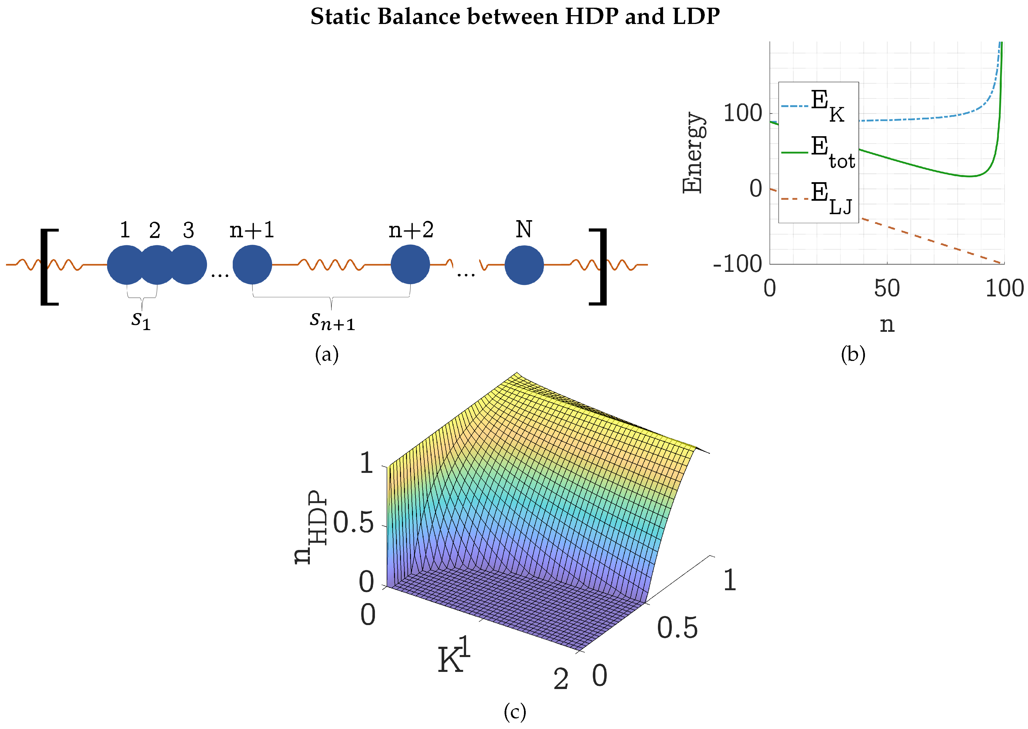
The phase separation of the gel can be explained with the competing LJ and harmonic energies. To do so, the toy model was simplified to a one dimensional string of N LJ particles connected through harmonic springs with one group of HDP particles and the rest LDP particles (see Figure 9). In this simplification, the effect of thermal vibrations is neglected - all HDP particles are assumed to be precisely in the LJ minimum at and . Therefore all HDP springs are of equal length . Further we assume the LDP springs to be spaced equally and to be larger than the LJ cutoff radius. Thus .
The LJ energy of the n HDP particles then is as only the LJ energies of the HDP particles is nonzero. The energy of the harmonic springs is
The graph of these two energies and their sum is given in Figure 9b. For particles, a spring coefficient of a density of and a box length of the total static energy has a minimum at .
Varying density and spring coefficient, a surface of minimal total static energy was found - giving for each combination of and K the optimal HDP particle fraction (see Figure 9c). This shows an energetic motivation for phase separation, driving the system towards an equilibrium state of minimal energy.
Considering one alteration of the model, the observed growth of the network can be explained: If we imagine not one, but several groups of HDP particles, for each new group created, one LJ bond is lost and replaced with a stretched spring, raising the total energy. The observed surface optimization is the reverse of this imagined process - decreasing the total energy through replacing long springs with LJ bonds.
4.2. Formation and Dissolution of HDP
To explain the influence of the temperature, and why sometimes phase separation occurred without the formation of a HDP network, let us consider an other one-dimensional model (see Figure 10a): One, mobile LJ particle is connected with two springs of lengths and to its neighbors which are at a fixed distance of to each other. A short calculation reveals the spring energy to be
where r denotes the distance of the moving particle from its left-hand-side neighbor. Together with the LJ potential, it follows that for , the total potential of the mobile particle is
Both energies and and the resulting total energy are plotted in Figure 10b.
Figure 10.
(a) Sketch of a LJ particle connected to two other fixed particles over harmonic springs with equilibrium length zero. The mobile particle is at a distance of to its left neighbor. (b) Harmonic spring energy , LJ energy and total energy of the mobile particle for with and .
Figure 10.
(a) Sketch of a LJ particle connected to two other fixed particles over harmonic springs with equilibrium length zero. The mobile particle is at a distance of to its left neighbor. (b) Harmonic spring energy , LJ energy and total energy of the mobile particle for with and .
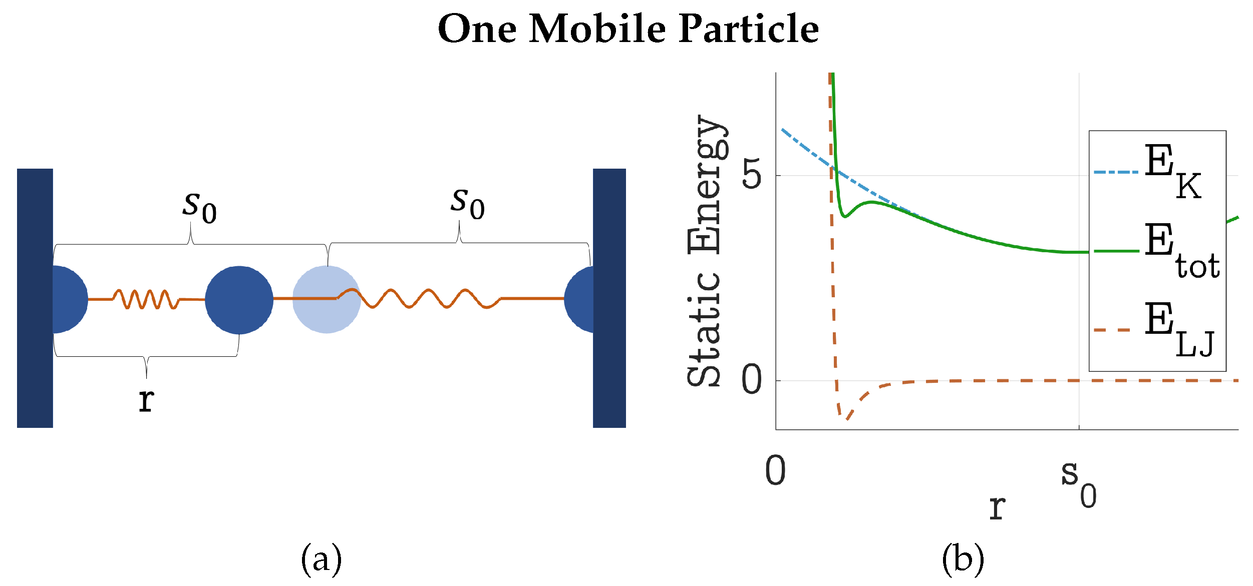
It can be observed, that in order to get to the LJ minimum, which is only a local minimum in the regarded example, the mobile particle needs to overcome a considerable energy barrier.
If we would extend this model to the right-hand-side, considering a second a third or more mobile particles, those particles could sometimes aid this first one with reaching the left LJ minimum by approaching or by accelerating it to the left, and other times keep it from reaching the LJ minimum by doing the opposite.
Exact calculations would need to be conducted through a statistical approach, considering the possible vibrations of the gel. For now the intuition must suffice: It is energetically adverse for one particle to reach the other if it is moving alone. It needs more energy, through either a higher temperature, or through neighboring particles vibrating collectively, which can be achieved by slightly increasing the spring coefficient. If there is too much thermal energy or if those neighbors vibrate too much, the particle is in danger of being ripped out of the LJ bond again.
This intuition can be applied to the phase diagrams found for the two- and three-dimensional gel models (see Figure 7 and Figure 8). At low temperatures and low spring coefficients, particles didn’t have enough vibrational energy to reach each other and form a network. Only small precipitates form (Region I). This could be remedied by reinforcing the connection between the particles by increasing the spring coefficient, to make them more likely to vibrate collectively and thus enabling the precipitates to form a network (region II). Too large spring coefficients then had the reverse effect, forcing the particles apart and dissolving the HDP again (region III). Another possibility of connecting the precipitates from region I was to increase the temperature directly, giving the particles more energy to bridge the gap between precipitates. Too large temperatures then dissolved the HDP again.
4.3. Future Works
Shorter simulation times, allowing more or larger simulations, would be very welcome for future projects. The most promising alternative to the rather slow MATLAB code was found in rewriting the simulation in Julia [12]. This way, a simulation speed improvement of factor nine could be achieved. More might be possible by improving the neighbors lists or by parallelizing the calculations.
Future works treating the same model could quantify the influence of simulation parameters ,T and K on morphology using the final measures from Section 2.4 (HDP surface fraction , HDP thickness , ...), to move away from describing the observed change in morphology from images as done in Section 3.2. This would remove subjectivity and allow possible automatization to e.g. find the parameters for the largest surface area.
For the same reason, fix, non-subjective criteria should be developed for associating gels to regions I, II and III.
One possibility would be, to use the small boxes covering the HDP volume (established in Section 2.4). Region II could be defined as a percolating structure of small boxes. This could be implemented with a forest fire algorithm like in [13,14]. Other suitable criteria could be found, taking a certain minimal HDP particle fraction combined with a minimal HDP thickness. Either would enable an automated mapping of phase diagrams like Figure 7 and Figure 8.
Instead of running simulations with constant parameters, outgoing from an initial state, simulations could be started from the final/asymptotic state of a simulation of other parameters. This would serve to further investigate the temperature hysteresis Peleg et al. [1] found, to see if a hysteresis could also be observed in the other two parameters ( and K), and if the same phase diagram would develop eventually.
The prediction for the optimal HDP particle fraction of a one-dimensional gel model (Section 4.1) could be compared to simulations of a one-dimensional gel model, and generalized to also include the influence of temperature.
To get closer to reality, the model could be altered by e.g. using a distribution of spring coefficients instead of a uniform K or by randomizing the structure through e.g. cutting/disabling some of the springs of the initial simple cubic lattice, as in [8]. Another approach would be to insert a second species of solvent particles.
The two-dimensional model of Peleg at al. [1,2] has already been compared to experimental results from investigating biopolymer mixtures in confined geometries [15] and found to be "in good agreement" with their findings.
An other direct link to observable gels might be achieved through changing the three-dimensional model to simulate a surface, by changing one dimension from periodic to non-periodic with a boundary against vacuum or LJ fluid. The resulting surface could then be compared to scanning electron microscopy (SEM) images or atomic force microscopy (AFM) images of gel surfaces like they were obtained in [16,17,18,19].
Alternatively, the resulting structure of larger three-dimensional simulations could be compared to gels investigated with micro-computed tomography (micro-CT) [20].
Funding
This research received no external funding.
Data Availability Statement
Data available upon request. Requests to access the datasets should be directed to the author.
Acknowledgments
I am grateful to my supervisor, Martin Kröger for giving me the opportunity to explore this beautiful toy model, and for trusting me, to work in such an independent fashion. Without his insightful feedback this paper would not be of the same quality – without his encouragement it would not exist. Further, I would like to thank Christophe Desarzens and Stefan Schären for their proofreading of this article and their very constructive feedback on my overcomplicated figures.
Conflicts of Interest
The author declares no conflicts of interest.
Appendix A
For a given particle, the neighbors list needs to contain at least all particles in a radius that could interact with it in a given time interval . Where the list is updated every -th time-step and is the cutoff radius above which the LJ potential is set to zero. A reasonable can be estimated as follows. Considering the MB distribution of the velocities, it is very unlikely for particles to have velocities exceeding . The probability for that is . Accounting for the relative movement of the particles with a factor of two this gives
where the mean speed is given by , which yields Eq. (1) as an estimate for the radius of the neighbors lists, ensuring that all LJ interactions are properly taken into account.
References
- Peleg, O.; Kröger, M.; Hecht, I.; Rabin, Y. Filamentous networks in phase-separating two-dimensional gels. Europhys. Lett. (EPL) 2007, 77, 58007. [Google Scholar] [CrossRef]
- Peleg, O.; Kröger, M.; Rabin, Y. Model of Microphase Separation in Two-Dimensional Gels. Macromolecules 2008, 41, 3267–3275. [Google Scholar] [CrossRef]
- Alvarez-Tirado, M.; Castro, L.; Guéguen, A.; Mecerreyes, D. Iongel Soft Solid Electrolytes Based on [DEME][TFSI] Ionic Liquid for Low Polarization Lithium-O2 Batteries. Batteries & Supercaps, p. e202200049. Available online: https://chemistry-europe.onlinelibrary.wiley.com/doi/pdf/10.1002/batt.202200049. [CrossRef]
- Chotsuwan, C.; Boonrungsiman, S.; Chokanarojwong, T.; Dongbang, S. Mesoporous soft solid electrolyte-based quaternary ammonium salt. Journal of Solid State Electrochemistry 2017, 21, 3011–3019. [Google Scholar] [CrossRef]
- Mozaffari, K.; Liu, L.; Sharma, P. Theory of soft solid electrolytes: Overall properties of composite electrolytes, effect of deformation and microstructural design for enhanced ionic conductivity. Journal of the Mechanics and Physics of Solids 2022, 158, 104621. [Google Scholar] [CrossRef]
- Xiao, H.; Li, H.; Wang, Z.L.; Yin, Z.N. Finite Inelastic Deformations of Compressible Soft Solids with the Mullins Effect. In Advanced Methods of Continuum Mechanics for Materials and Structures; Naumenko, K., Aßmus, M., Eds.; Springer, Singapore: Singapore, 2016; pp. 223–241. [Google Scholar] [CrossRef]
- Sekimoto, K.; Suematsu, N.; Kawasaki, K. Spongelike domain structure in a two-dimensional model gel undergoing volume-phase transition. Phys. Rev. A 1989, 39, 4912–4914. [Google Scholar] [CrossRef] [PubMed]
- Peleg, O.; Kröger, M.; Rabin, Y. Effect of network topology on phase separation in two-dimensional Lennard-Jones networks. Phys. Rev. E 2009, 79, 040401. [Google Scholar] [CrossRef] [PubMed]
- Thompson, A.P.; Aktulga, H.M.; Berger, R.; Bolintineanu, D.S.; Brown, W.M.; Crozier, P.S.; in ’t Veld, P.J.; Kohlmeyer, A.; Moore, S.G.; Nguyen, T.D.; et al. LAMMPS - a flexible simulation tool for particle-based materials modeling at the atomic, meso, and continuum scales. Comput. Phys. Comm. 2022, 271, 108171. [Google Scholar] [CrossRef]
- Schultz, A.J.; Kofke, D.A. Comprehensive high-precision high-accuracy equation of state and coexistence properties for classical Lennard-Jones crystals and low-temperature fluid phases. The Journal of Chemical Physics 2018, 149, 204508. [Google Scholar] [CrossRef] [PubMed]
- Stephan, S.; Staubach, J.; Hasse, H. Review and comparison of equations of state for the Lennard-Jones fluid. Fluid Phase Equilibria 2020, 523, 112772. [Google Scholar] [CrossRef]
- Bezanson, J.; Edelman, A.; Karpinski, S.; Shah, V.B. Julia: A fresh approach to numerical computing. SIAM review 2017, 59, 65–98. [Google Scholar] [CrossRef]
- Albinet, G.; Searby, G.; Stauffer, D. Fire propagation in a 2-D random medium. Journal De Physique 1986, 47, 1–7. [Google Scholar] [CrossRef]
- Stauffer, D.; Aharony, A. Introduction To Percolation Theory: Second Edition; Taylor & Francis, 1992. [CrossRef]
- Fransson, S.; Peleg, O.; Lorén, N.; Kröger, A.H.M. Modeling and confocal microscopy of biopolymer mixtures in confined geometries. Soft Matter 2010, 6, 2713–2722. [Google Scholar] [CrossRef]
- Kaberova, Z.; Karpushkin, E.; Nevoralová, M.; Vetrík, M.; Šlouf, M.; Dušková-Smrčková, M. Microscopic Structure of Swollen Hydrogels by Scanning Electron and Light Microscopies: Artifacts and Reality. Polymers 2020, 12. [Google Scholar] [CrossRef] [PubMed]
- Hagmann, K.; Bunk, C.; Böhme, F.; von Klitzing, R. Amphiphilic Polymer Conetwork Gel Films Based on Tetra-Poly(ethylene Glycol) and Tetra-Poly(ϵ-Caprolactone). Polymers 2022, 14. [Google Scholar] [CrossRef] [PubMed]
- Damaschin, R.P.; Lazar, M.M.; Ghiorghita, C.A.; Aprotosoaie, A.C.; Volf, I.; Dinu, M.V. Stabilization of Picea abies Spruce Bark Extracts within Ice-Templated Porous Dextran Hydrogels. Polymers 2024, 16. [Google Scholar] [CrossRef] [PubMed]
- Dimic-Misic, K.; Imani, M.; Gasik, M. Effects of Hydroxyapatite Additions on Alginate Gelation Kinetics During Cross-Linking. Polymers 2025, 17. [Google Scholar] [CrossRef] [PubMed]
- Cengiz, I.F.; Oliveira, J.M.; Reis, R.L. Micro-CT – a digital 3D microstructural voyage into scaffolds: a systematic review of the reported methods and results. Biomaterials Research 2018, 22. [Google Scholar] [CrossRef] [PubMed]
Figure 1.
(a) Three-dimensional model of the gel: Simple cubic lattice of LJ particles connected with harmonic springs of equilibrium distance zero, subjected to periodic boundary conditions. (b) Two-dimensional gel model simulation after a time of with density , temperature and spring coefficient . The springs connecting HDP particles are highlighted in orange for the graphical representation. (c) Three-dimensional gel model simulation after a time of with simulation parameters , and . In this graphical representation, the springs are colored according to their spatial orientation.
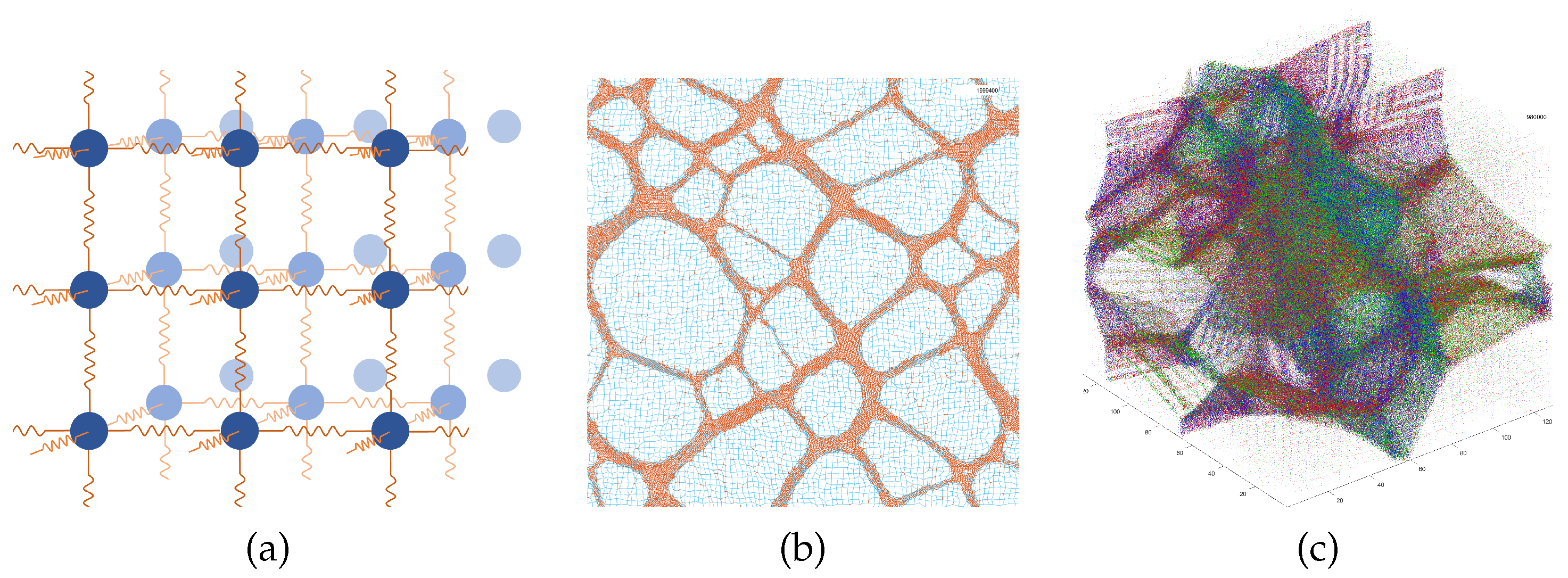
Figure 2.
Process of surface measurement of the HDP network of a gel in two and three dimensions. First HDP particles are determined. Then all HDP particles which don’t fall under the criterion for random agglomerates are put into small blue cubes (yellow squares). From there the surface is beset with big violet surface cubes (green surface squares), which have the criterion to be partially comprised of small cubes/squares present.
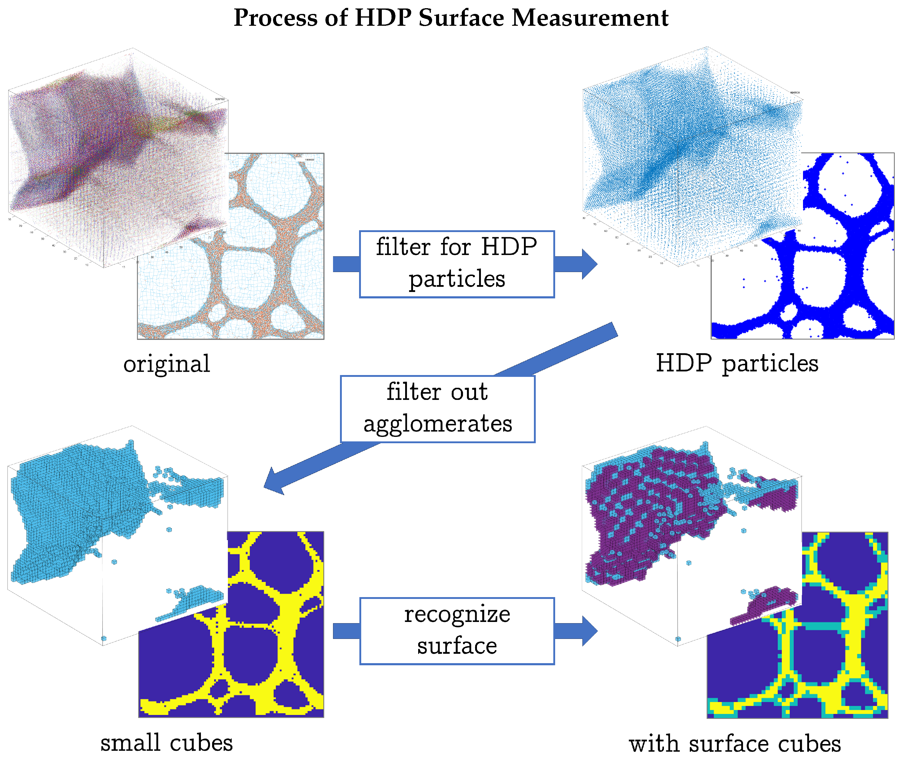
Figure 3.
Gel simulations of the two- and three-dimensional model at different points in time t. In both cases, fast phase separation followed by the slower formation of a complex HDP network can be observed. The two-dimensional gel model was simulated with particles, at constant density , temperature and spring coefficient . The springs belonging to HDP particles were colored orange. The three-dimensional gel simulation was run with particles, at constant density , temperature and spring coefficient . Here all springs were colored according to their spacial orientation.
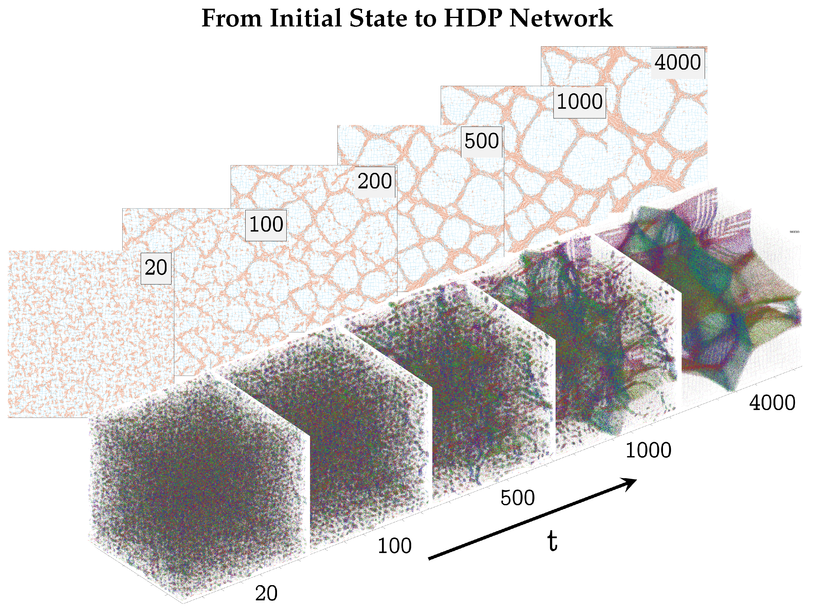
Figure 4.
Evolution of the three-dimensional gel depicted in Figure 3 described by the measures established in Section 2.4. The gel simulation was run with particles, at constant density , temperature and spring coefficient . (a) shows HDP density , HDP particle fraction and HDP volume fraction over time. (b) shows the evolution of HDP filament thickness together with HDP area fraction and HDP volume fraction over time. And (c) shows the change in spring energy , LJ energy and their sum .
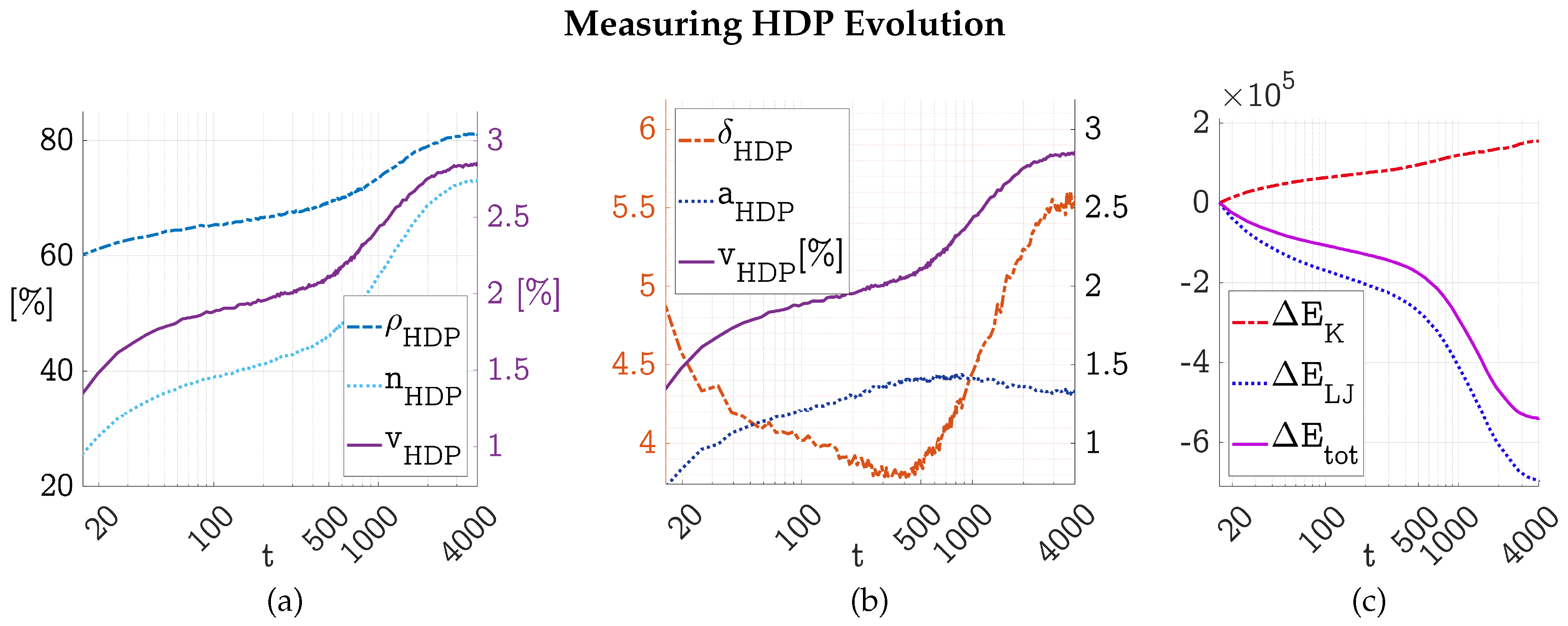
Figure 5.
Evolution of the morphology (MPD, SLD and RSD) of the three-dimensional gel simulation depicted in Figure 3. In all three plots, the dashed-dotted black line at indicates the minimum of the LJ potential. The blue dashed line in the MPD at separates HDP from LDP particles. In the RSD additional lines indicate the first three peaks of a bcc- and fcc structure with minimal distance of respectively. The gel simulation was run with particles, at constant density , temperature and spring coefficient .
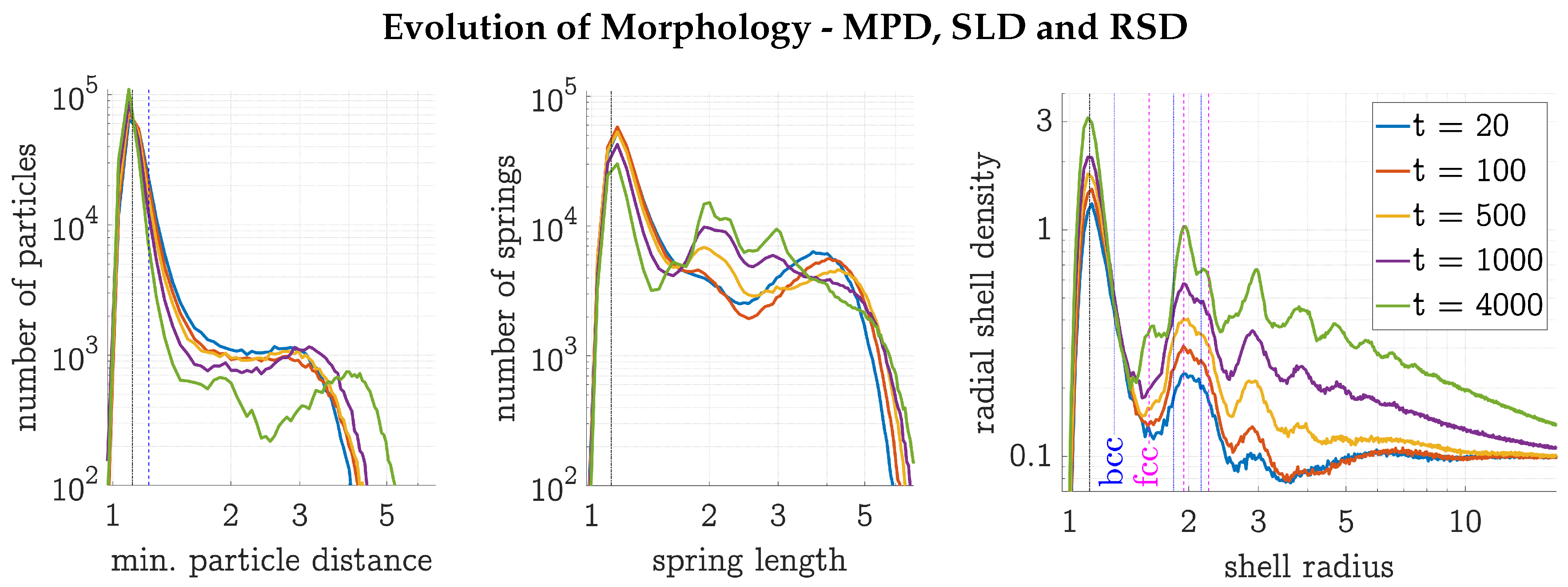
Figure 6.
Final state () of the gel simulations with one varying parameter (density , temperature T or spring coefficient K) while the other two parameters remained constant. Upper/2D simulations were conducted with particles and with if not specified. The lower/3D simulations with and with constant , if not specified. One simulation was conducted for each set of parameters.
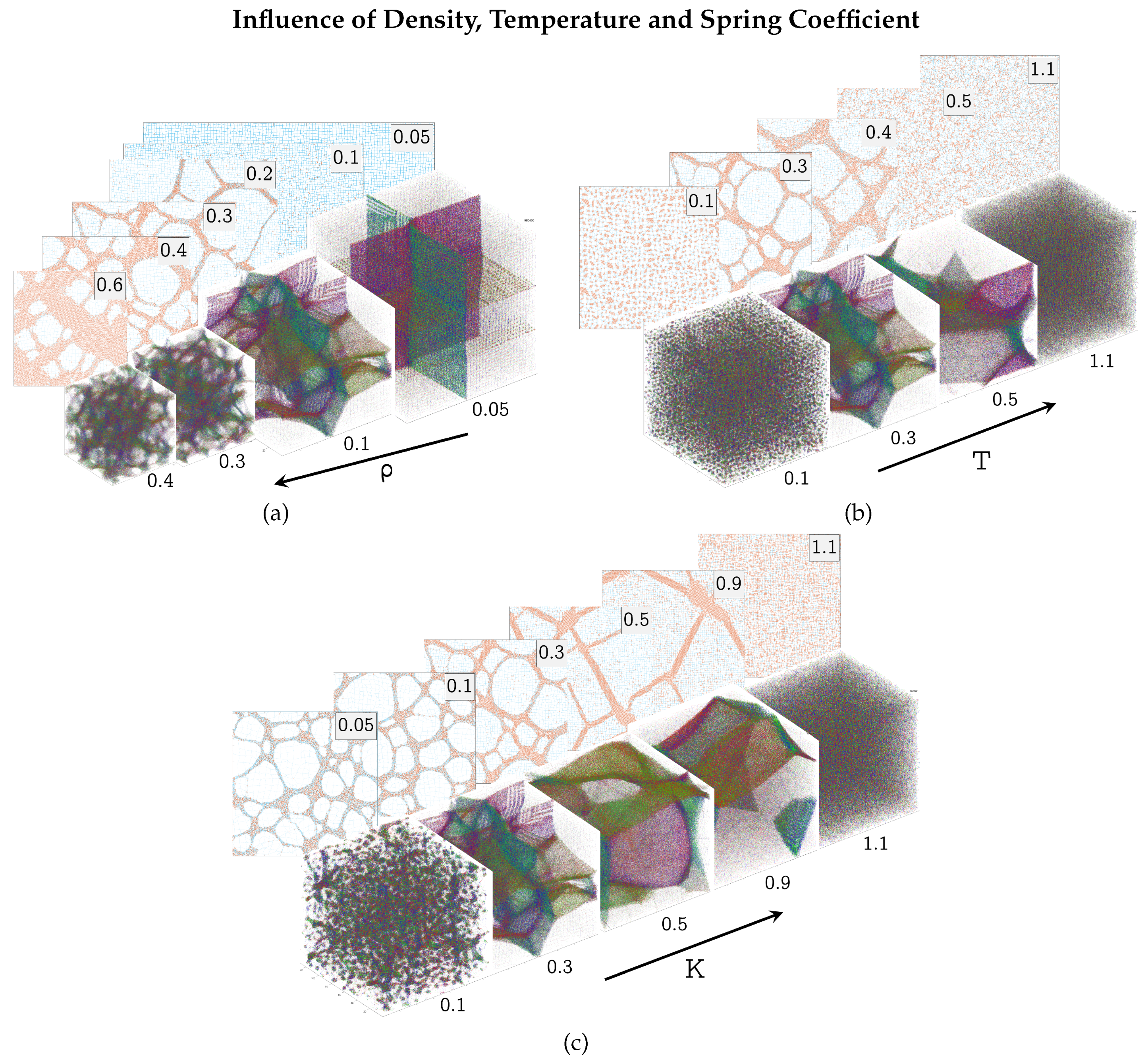
Figure 7.
Phase diagram of the three-dimensional gel model at constant density . The solid blue line separates the upper right single phase region III from the lower left regions I and II, where phase separation into HDP and LDP was observed. The dashed blue line further divides simulations, where HDP networks were observed (blue rings/region II) from those, where only HDP precipitates formed (region I).
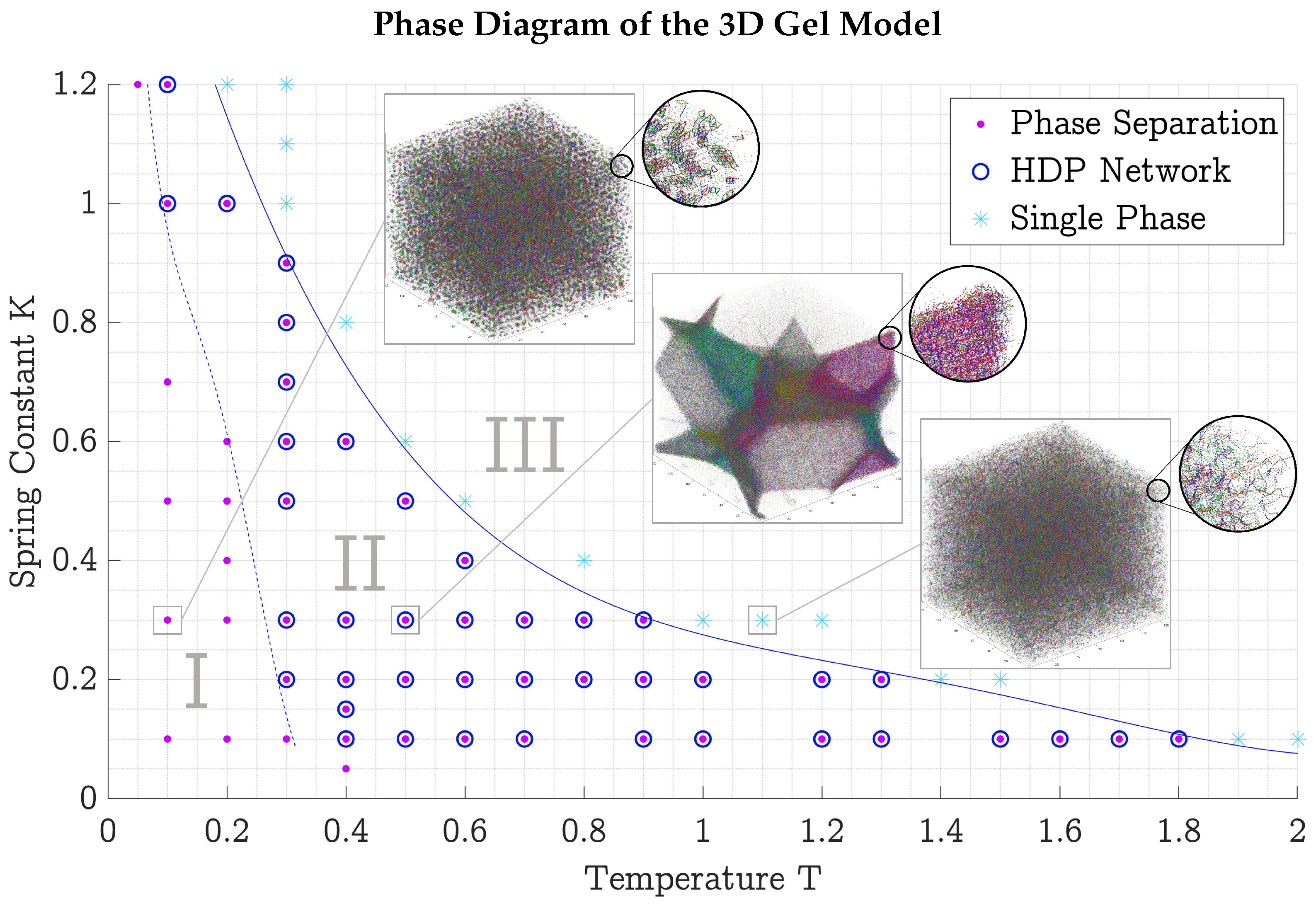
Figure 8.
Phase diagrams of the two-dimensional gel model at constant densities , and from left to right. The same three regions as in the phase diagram of the three-dimensional model (Figure 7) could be observed. The solid blue line separates single phase region III from the lower left regions I and II. The dashed blue line further divides these into region II, where HDP networks could be observed, and region I, where only HDP precipitates formed.
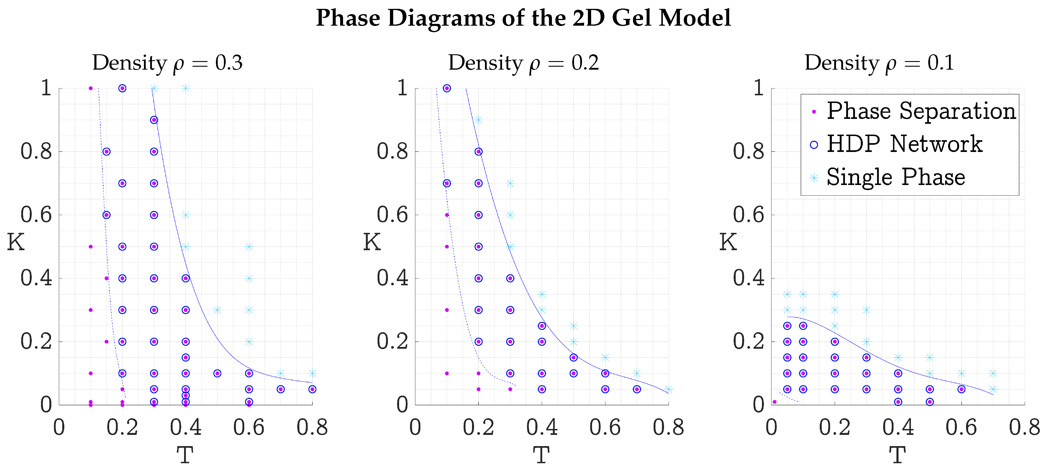
Figure 9.
(a) Sketch of a one dimensional simplification of the gel model with particles 1 to in each others LJ potential grouped together as HDP and particles to N as LDP. The distances between the particles are denoted with for e.g. the distance between particle n and particle . The brackets stand for the PBC. (b) Quantitative plot of the total static energy of the one dimensional model sketched in (a) as the sum of the LJ energy and the harmonic spring energy . Here with particles, spring coefficient , density and a box length of . The total static energy has a minimum at . (c) Surface of minimal total energy in the space spanned by density , spring coefficient K and HDP particle fraction for the one dimensional model sketched in (a).
Disclaimer/Publisher’s Note: The statements, opinions and data contained in all publications are solely those of the individual author(s) and contributor(s) and not of MDPI and/or the editor(s). MDPI and/or the editor(s) disclaim responsibility for any injury to people or property resulting from any ideas, methods, instructions or products referred to in the content. |
© 2025 by the authors. Licensee MDPI, Basel, Switzerland. This article is an open access article distributed under the terms and conditions of the Creative Commons Attribution (CC BY) license (http://creativecommons.org/licenses/by/4.0/).
Copyright: This open access article is published under a Creative Commons CC BY 4.0 license, which permit the free download, distribution, and reuse, provided that the author and preprint are cited in any reuse.


