Submitted:
11 February 2025
Posted:
11 February 2025
You are already at the latest version
Abstract
We model the energy depletion of light from a distant object with two components: loss in photon rates (number of photons) and loss per photon particle. We model the rate loss based on intergalactic extinction, which, unlike extinctions within our local group of Milky Way, LMC and SMC, has not been previously accounted for. Ignoring intergalactic extinction results in overestimation of cosmic distances with standard distance moduli. Such extinction effect is more profound on large scales (Gpc) that we have only started to observe today. We then apply the tired light model for energy loss (redshift) per photon. These two model components are mathematically very simple, leading to a new equation between luminosity distance and redshift. The model performed equally well as ΛCDM with Pantheon+ SN data while outperformed it with deep-field galaxy angular size test. The main implications of the intergalactic extinction model are two-fold: it identifies a major bias in distance measurements based on standard candles; it is also a key missing piece for static universe models to offer as viable alternatives to ΛCDM. Thus, the model has further implications on the interpretation of cosmic redshift, Hubble’s law, the Hubble constant, Hubble tension, and universe history.
Keywords:
intergalactic extinction
; ΛCDM
; static model
; Hubble tension
1. Introduction
ΛCDM is currently the standard model of cosmology. It’s success, however, has been challenged recently by HST and JWST observations in the model’s early universe billions of light years away. Multiple mature galaxies were reported [1,2,3], which are not predicted by the standard model. The Hubble tension further highlights the difficulty facing ΛCDM if data measurement issues are not the culprit. These have prompted some to call for new physics, e.g. [4]. This paper presents a simple model to account for extinctions in vast intergalactic space. We discuss the proposed intergalactic extinction model in combination with the tired light model, which together had performed equally well as ΛCDM with Pantheon+ SN data and outperformed it with galaxy angular size data, in support of a static universe model over ΛCDM making the Hubble tension irrelevant and deep space mature structures explainable. In sections 2, we propose a simple model of light energy depletion through intergalactic extinction and energy redshift. The two components together are necessary to describe energy behaviors throughout the light’s travel path. Section 3 discusses previous estimation results and fitness of the proposed model vs. ΛCDM to the data. Conclusion is in section 4.
2. Materials and Methods
2.1. The Energy Depletion Model of Light
Without loss of generality, we decompose and write the flux received on earth from a beam of light with wavelength λ as
E = NEλ
where N = N0/4πd2
is the number of photons per square area per time unit, d is the true distance (or the proper distance in an expanding universe) from the emitter, N0 is the number of photons emitted by the emitter per time unit; and
Eλ = hc/λ
is the energy per photon, and h is the Planck constant. Also Eλ0=hc/λ0 where λ0 and Eλ0 are the wave length and energy per photon at source.
2.2. The Intergalactic Extinction Model
Interstellar and host (or internal, extragalactic) extinctions have been studied extensively close to earth on MW, LMC and SMC, and on host galaxies respectively. It has been essential to apply corrections to distance moduli to account for such extinctions when estimating distances or the intrinsic brightness of the source. Brout and Riess [5] give a comprehensive review on these extinctions. However, similar types of extinctions due to intergalactic media in between the host galaxy and MW/LMC/SMC along the vast distances of light travel has not been accounted for, which should increase with distance and thus become increasingly critical as our modern telescopes look into deeper space on the Gpc scale, resulting in overestimation of distances.
Intergalactic extinctions (IEs) may occur after the emitted light of a star leaves its host galaxy and before it enters the LMC/SMC/MW range. IE increases with distance, and may come from three sources:
- the light may encounter more galaxies or be “blocked” by them in our line-of-sight;
- it may encounter edges of galaxies or circumgalactic medium (CGM);
- it may encounter Warm-Hot intergalactic medium (WHIM) or Intracluster medium (ICM), and a great majority of baryonic matters in the universe too dimmed to be seen yet by existing telescopes (Massimo and Salucci [6]).
To gauge on the significance of intergalactic extinction source 1 above, Let’s do a rough estimation by answering the question: how likely would one expect to have a galaxy or galaxies in the line-of-sight between the light source and an earth observer? It’s a battle of two sheer numbers: the very large number of galaxies in the very large volume of the universe. Detailed in the Appendix A, the answer is: 6% probability per Gpc if the source is a galaxy, and 25% probability per Gpc if the source is a star (Cepheid, Supernova etc). These conservatively estimated probabilities are significant and must not be ignored.
Unlike interstellar and host extinctions, intergalactic extinction cannot be estimated with extinction curves since there is no photometric nor spectroscopic data available for unidentified extinction media. However, we can still model and estimate its effect statistically. We now apply the exponential decay function e-2d/D to the photon rate in Eq. (2): N=(N0/4πd2)*e-2d/D = N0/4π(ded/D)2 with the decay coefficient written as 2/D for subsequent convenience. Thus, the intergalactic extinction (IE) model can be written simply as
dL(d) = ded/D
where dL is the indirectly measurable luminosity distance and D is a constant. D/2 is the distance by which 36.8% (1/e) photons remain alive from extinction, or the mean life-distance (analogue to mean lifetime for decays over time) of photons. (D was estimated to be 21.0 Gly with the Pantheon+ SN data as discussed in section 3 below.)
Figure 1 shows the behavior of dL versus d under three different parameter values of D=13, 21, 29 Gly, and dL=d as D->∞. The luminosity distance dL approximates the true distance d well for small distance (d<<D) but deviates upwards exponentially.
It is important to note that only dL can be calculated with the distance modulus m-M=5logdL-5. The true distance d in a static universe (or the proper distance in an expanding universe) can only be calculated after the parameter D is estimated. These properties of dL and d are independent of cosmological models, expanding or static. In the case of expanding universe models such as ΛCDM, the distance modulus overestimates the proper distance d with dL, unless corrections are made to the modulus formula; and further, Hubble’s law is the ratio of recession velocity to the measured luminosity distance, and not to the proper distance. Since v=H0dL, we can place velocity v on the vertical axis in Figure 1 which implies that the universe is decelerating instead of accelerating as the v-d curve is above the straight v=H0d (or dL=d). One may conclude an accelerating universe by using dL but that is delusional as dL is an overestimation.
2.3. The Redshift Model
Similar to the IE model, to model the light energy depletion due to redshift of each photon in the light, we apply the exponential decay function e-d/Δ to Eq. (3): Eλ=Eλ0*e-d/Δ, or λ= λ0ed/Δ. Since λ=λ0(1+z),
z(d) = ed/Δ-1
or d = Δln(1+z)
where Δ is a constant. For d<<Δ and d<<D, with Taylor expansions, Eq. (4) and (5) reduce to dL=d and z=d/Δ. Thus, we have Hubble’s law z=dL/Δ in which Δ=c/H0 and H0 is the Hubble constant, and Δ13.8 Gly is in fact the familiar Hubble distance. Given an observed value of z, the true distance to the light source can also be calculated simply with Eq. (5’). The observed dL is very useful for estimation purposes but is not the true distance and is delusional as it does not take intergalactic extinction into account. Zhang [7] offered an additional and interesting explanation of the physics at play for photons to redshift over distance.
Under this model, for each Hubble distance Δ traveled, the photon’s wave length is redshifted by e-1 (~1.72) or the associated photon energy remaining is 1/e (~36.8%). Δ is also the expected value of distance weighted by the energy level as probability density during a photon's entire trip from distance zero to infinity. While Δ=Hubble distance, it does not have the same interpretation here as under the expanding universe hypothesis as there is no expanding space and recession velocity in a static universe.
2.4. The Combined Empirical Model
Figure 2 shows the functions dL(d) and z(d) graphically. Substituting Eq. (5’) into Eq. (4), we obtain the empirical dL-z relationship:
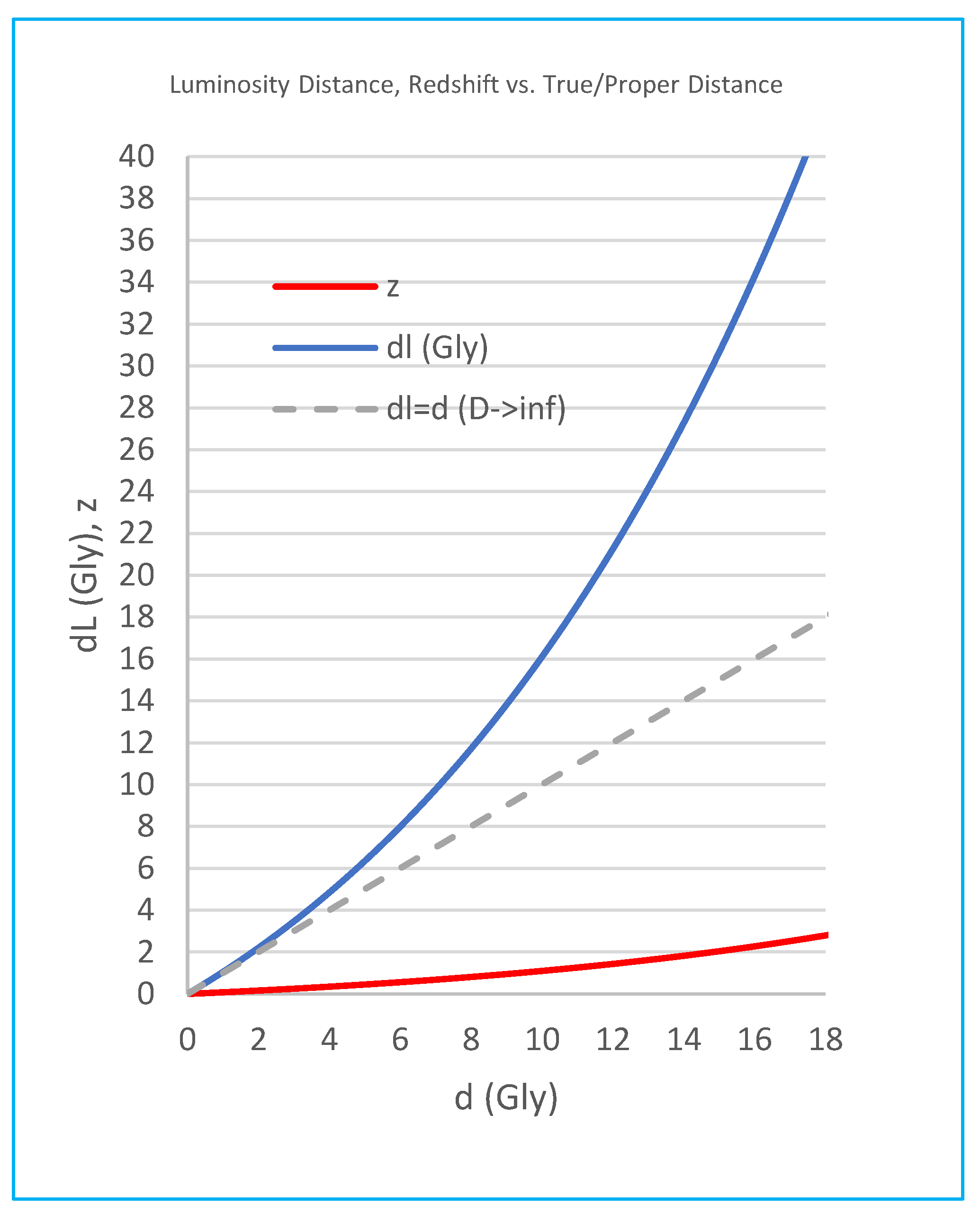
Figure 2.
the functions dL(d) at D=21Gly, and z(d).
dL = Δ(1+z)Δ/Dln(1+z).
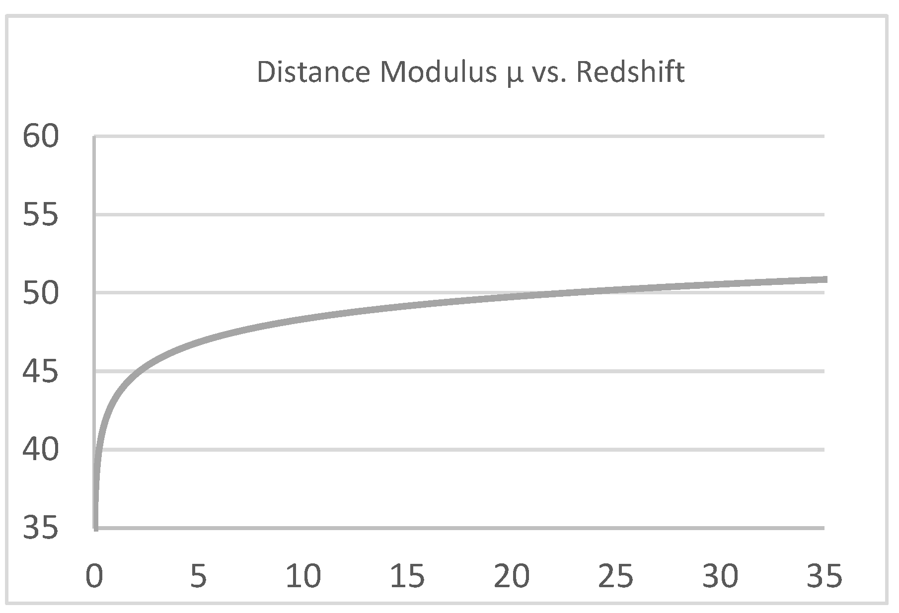
In terms of the distance modulus μm-M=5logdL-5,
μ = 5(logΔ-1)+5(log(ln(1+z))+log(1+z)Δ/D).
Eq. (6) and (7) are equivalent and have two parameters, Δ (or H0=c/Δ) and D (or Δ/D), which can be empirically estimated. (The total flux can also be written as E(d)=E0e-d(1/Δ+2/D) where E0 is energy at source.) Figure 3 and Figure 4 shows the graphs of Eq. (6) and (7) respectively. The dL-z relationship is a s-curve1 closely approximating the straight dL=Δz or Hubble’s law, with deviations 13.4% over 0z125 (for Δ=13.5 Gly and D=21 Gly taken from empirical estimation discussed in section 3 below). In other words, the luminosity distance per unit (100%) of redshift is roughly 13.5 Gly.
Note also the symmetry between Eq. (4) and (5) in terms of dL/d and λ/λ0(=1+z). We may call rλλ/λ0 the redshift ratio, and rddL/d the dimshift ratio (as the light is shifted dimer by extinction). We take first derivatives with respect to d in (4) and (5) and get
Drd’/rd = Δrλ’/rλ = 1, and rλrd’/rdrλ‘ = Δ/D
Thus, Δ/D (0.64 per Pantheon+ SN sample) can be interpreted as the percentage change in the dimshift ratio as one percentage change in the redshift ratio or in wavelength λ.
3. Results and Discussions
The two simple equations (4) and (5) are all we need to describe a static universe consistent with Hubble’s Law without the complicated ΛCDM model assuming expansion of space accelerated by dark energy. The two equations combine to produce Eq. (6) or (7) which can be empirically applied with z directly measured and dL indirectly via the distance modulus. The true distance, d, is not measurable outside the model and is a confounding exogeneous variable that affect both dL and z through Eq. (4) and (5) respectively. In this static universe, there is no space expansion and acceleration, no dark energy to search for (which one will never find if it doesn’t exist outside the hypothetical world of the standard model), not even age of the universe, beginning of time, nor the big bang. We will not be surprised to see JWST and other future telescopes continue to find more mature galaxies and structures in unbound distances.
Gupta [8] discussed the ΛCDM model and several alternative models including a TL+ model where an arbitrary or unknown flux loss term 5log(1+z)β was added to the distance modulus formula. This TL+ model is indeed the exact same model mathematically as the one proposed here (Eq. (7)) in that the TL+ parameter β=Δ/D. So, thanks to Gupta, the proposed model was already tested with the Pantheon+ SN data which showed an excellent fit as good as the ΛCDM model with estimated H0=72.46 Km s-1 Mpc-1 and β=0.6418, and thus Δ=c/H0=13.5 Gly and D=Δ/β=21.0 Gly. Gupta further tested the models with galaxy angular size data and found that the TL+ or the proposed model’s fit was acceptable for high redshift while the standard ΛCDM model was not, which may be a smoking gun in favor of the proposed model over ΛCDM. Although Gupta included the TL+ model for discussion purpose only, it in fact turned out to explain the data equally well as or better than ΛCDM. For detailed results of the proposed model fitted with the data, please refer to the TL+ model in Gupta. Note that Zhang’s model is also the same but the β parameter there was given a value of 1.2 before fitting the SCP Union SNIa data. Both papers added the β-term somewhat arbitrarily to tired light models or otherwise the models were inadequate. The missing piece to previous redshift or tired light models is in fact the extinction equation (4). No arbitrary term is needed. Again in cosmology, the dust tricked us.
From Eq. (4), the relative bias of dL as a measure of d is given by dL/d-1=ed/D-1. For d<<D, this bias is approximately d/D, and thus is linear and small, For example, at d=1%D210 Mly, the bias is only 0.005%. When dL approaches D, the bias grows exponentially and dominate. At d=D21 Gly, the bias is a whopping e-1=172%! Thus, any focus on achieving a small measurement uncertainty as in the case of estimating the Hubble constant using the distance ladder method for Hubble tension discussions, is irrelevant if one ignores the biggest bias of all – intergalactic extinction. It is surreal to claim that the total measurement errors can be so small when measuring vast distance of space still full of many unknowns and measuring it indirectly through source brightness.
4. Conclusions
The proposed IE model is independent of cosmology models and may coexist with ΛCDM. However, the IE model also implies that the Hubble tension is an artifact in that the luminosity distance dL in Hubble’s law used for estimation is subject to intergalactic extinction, and is not the true or proper distance d. It thus identifies a major bias for distance and H0 local measurements using standard candles and other luminosity-based methods. It implies both H0 measurement errors and (not so) new physics in the context of Hubble tension discussions. Additionally, given ΛCDM together with the IE model, the universe is not accelerating and is decelerating instead.
The IE model also provides the missing piece of the puzzle to tired light theories and explains the deep space data equally well as or better than ΛCDM. Why marginalize a simple static model in favor a complex expanding-universe model, particularly in light of increasing observations in deep space favoring the former over the latter as well as the addition of the proposed IE model here?
It is not a sound argument to refute the tired light model on the ground that there is no knowledge in physics for photons to redshift over distance. The evidence of such knowledge is unobtainable independently in lab or in nature as it would require distances in millions of light years to conduct such an experiment, which is the exact observations that the proposed model here and others do predict. This can be seen easily from Hubble’s law z=dL/13.8 Gly: a distance of 138 Mly (or 138 million years in scientists’ life to observe) is required to detect z=0.01, 13.8 Mly to detect z=0.001, etc. The “decay” rate of energy redshift, i.e., the Hubble distance Δ, is just too large.
In my opinion as an outsider, it is just a matter of time that the cosmology community must reconsider a better alternative to the FLRW metrics and the ΛCDM model. The standard model of cosmology today strikes me as very puzzling to say the least. The claims of high precision in distance measurements are also surreal. The standard model has encountered and will very likely continue to encounter more contradictory evidence in deeper space, and I don’t believe that bandages to patch it are the solution.
Funding
This research received no external funding.
Conflicts of Interest
The author declares no conflicts of interest.
Appendix A: Rough Estimation of Line-of-Sight Probabilities
Imagine a squared galaxy of dimension r at a distance d (both in Mpc) from earth emitting light. (Squared galaxy rather than spiral or elliptical is chosen for convenience as we care about only the estimated magnitude.) With earth at the center, the ratio of the number (Nd) of galaxies inside the sphere of radius d to the number (Ns) of galaxies of dimension r which fully covers the sphere will yield the average number (nR) of galaxies in the line-of-sight: nR= Nd/ Ns. The dimensional diameters of galaxies are 10-3 to 10-1 Mpc. Let’s use the average r=10-2 Mpc. Then Ns=4πd2/r2105 d2/Mpc2.
The most recent estimates for the number of galaxies inside the observable universe of radius 14 Gpc are 6-20 trillions. Let’s take 10 trillion. Then Nd=1013d3/1400034d3/Mpc3. Therefore nR4*10-5d/Mpc =0.04d/Gpc, or Probg=nR/d=4%/Gpc, a 4% probability that a galaxy will be entirely in the line-of-sight of a source galaxy per Gpc. We can further refine this probability since the galaxy line-of-sight is cone-shaped, so the blocking galaxy is more than entirely covering the host galaxy. On average, the blocking galaxy may even sit at the median distance in terms of volume, so a factor of 1/( )21.6 can be applied to obtain final Probg=6.4%/Gpc.
Next, we calculate the probability, Probs, that the light from a single star (such as SNIa or Cepheid for typical distance measurements) inside the host galaxy being blocked by a galaxy along the travel path. Consider the squared host galaxy is 1x1 in area, then a small square of area=(Probg)1/2x(Probg)1/2 can be used to derive Probs=4Probg using a square of 2(Probg)1/2x2(Probg)1/2 centered at the star since this square is the area to ensure blocking the star. Therefore, Probs≈25%/Gpc. This means a very significant effect of intergalactic extinction but it is still an underestimation as it will go up when we further take into account CGM, WHIM, ICM, and other unseen or unknown baryonic matters in space.
| 1 | Let β=Δ/D. From Eq. (4), the second derivative dL’’= Δ(1+z)β-2[2β-1+ β(β-1)ln(1+z)]. So, (a) dL’’>0 for β1; (b) dL’’<0 for β½; and (c) dL’’0 iff ze(2β-1)/(β(1-β))-1 for ½<β<1 which is a s-curve but the curve shape is inconsequential because it is very close to the straight Δz. |
References
- Curtis-Lake, E., Carniani, S., Cameron, A. et al. Spectroscopic confirmation of four metal-poor galaxies at z = 10.3–13.2. Nat Astron 7, 622–632 (2023). [CrossRef]
- Labbé, I., van Dokkum, P., Nelson, E. et al. A population of red candidate massive galaxies ~600 Myr after the Big Bang. Nature 616, 266–269 (2023). [CrossRef]
- Robertson, B.E., Tacchella, S., Johnson, B.D. et al. Identification and properties of intense star-forming galaxies at redshifts z > 10. Nat Astron 7, 611–621 (2023). [CrossRef]
- Charles L. Steinhardt et al. The Highest-redshift Balmer Breaks as a Test of ΛCDM 2024 ApJ 967 172. [CrossRef]
- Brout, D., Riess, A. (2024). The Impact of Dust on Cepheid and Type Ia Supernova Distances. In: Di Valentino, E., Brout, D. (eds) The Hubble Constant Tension. Springer Series in Astrophysics and Cosmology. Springer, Singapore. [CrossRef]
- Massimo Persic, Paolo Salucci, The baryon content of the Universe, Monthly Notices of the Royal Astronomical Society, Volume 258, Issue 1, September 1992, Pages 14P-18P. [CrossRef]
- Zhang, T.X. (2018), Mach’s Principle to Hubble’s Law and Light Relativity. Journal of Modern Physics, 9, 433-442. [CrossRef]
- Rajendra P Gupta (2023), JWST Early Universe Observations and ΛCDM cosmology, Monthly Notices of the Royal Astronomical Society, Volume 524, Issue 3, September 2023, Pages 3385-3395. [CrossRef]
Figure 1.
the function dL(d) at different D values.
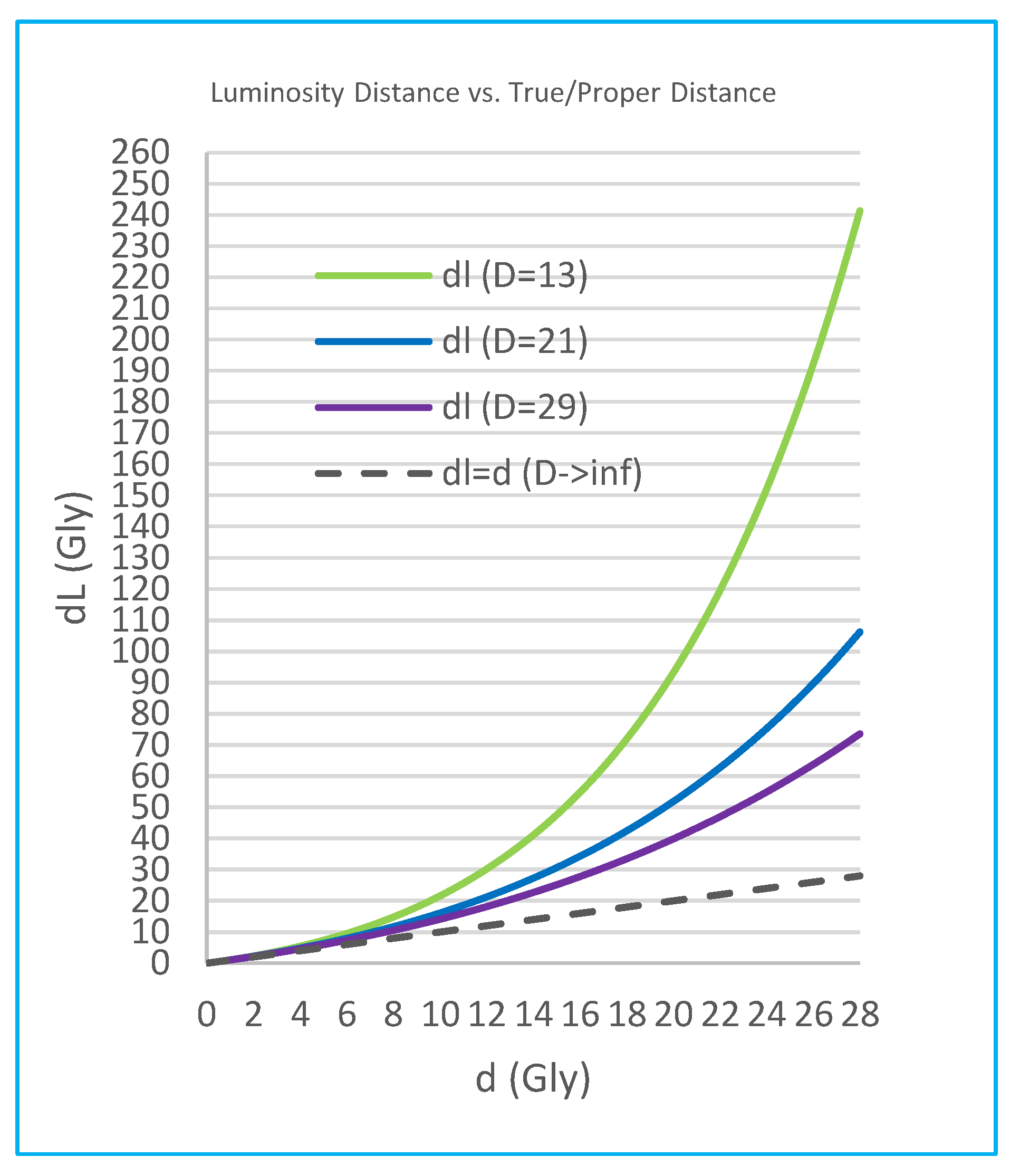
Figure 3.
the luminosity distance - redshift relation.
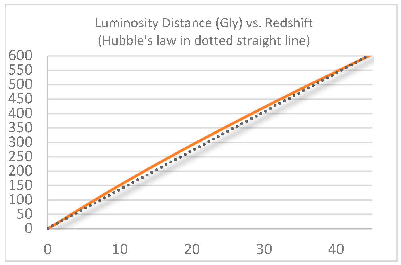
Figure 4.
the distance modulus - redshift relation.
Disclaimer/Publisher’s Note: The statements, opinions and data contained in all publications are solely those of the individual author(s) and contributor(s) and not of MDPI and/or the editor(s). MDPI and/or the editor(s) disclaim responsibility for any injury to people or property resulting from any ideas, methods, instructions or products referred |
© 2025 by the authors. Licensee MDPI, Basel, Switzerland. This article is an open access article distributed under the terms and conditions of the Creative Commons Attribution (CC BY) license (http://creativecommons.org/licenses/by/4.0/).
Copyright: This open access article is published under a Creative Commons CC BY 4.0 license, which permit the free download, distribution, and reuse, provided that the author and preprint are cited in any reuse.


