
Submitted:
08 February 2025
Posted:
11 February 2025
You are already at the latest version
Abstract
The discrete version of the Biswas-Chatterjee-Sen model, defined on D-dimensional hypercubic Solomon networks, with 1≤D≤6, has been studied by means of extensive Monte Carlo simulations. Thermodynamic-like variables have been computed as a function of the external noise probability. Finite-size scaling theory, applied to different network sizes, has been utilized in order to characterize the phase transition the system presents in the thermodynamic limit. It has been noticed that the model undergoes a second-order phase transition for all considered dimensions. Despite the lower critical dimension being zero, this dynamical system seems not having any upper critical dimension, since the critical exponents change with D and go away from the expected mean-field values. Although larger networks could not be simulated because the number of sites drastically increases with the dimension D, the scaling regime has been achieved when computing the critical exponent ratios. However, logarithm corrections to scaling are present when analyzing the behavior of the critical noise probability.
Keywords:
nonequilibrium
; phase transition
; Monte Carlo simulations
; Solomon networks
; lower upper critical dimension
1. Introduction
The critical properties of a system undergoing a second-order phase transition is strongly dependent on the dimension of the underlying lattice. In fact, the lattice dimension is one of the crucial factors to determine the universality class of a particular second-order phase transition (the other factors consist of the dimension of the order parameter and symmetry and range of the particle interactions). The renormalization group theory turned out to be a successful framework to understand the universal aspects of the critical phenomena from the knowledge of the basic microscopic interactions (see, for instance, Ref. [1] and references therein).
It is also well established in the literature that each system has its proper lower critical dimension , below which there is no phase transition, and also an upper critical dimension , above which the transition is governed by the mean-field exponents [2]. Of course, the upper critical dimension has only a theoretical interest, because is usually above the three-dimensional space of the physical sample realizations [3]. Just to cite some examples, we have and for the Ising model [1], and for the isotropic Heisenberg model [1], [4] and [5] for the Ising spin-glass system. More recently, it has been reported that and for the majority vote model on regular lattices [6].
The magnetic models cited above, defined on regular Bravais lattices, are well studied in the literature because they are in some sense easier to define, suitable to being simulated using different sort of computer algorithms, and with plenty physical realizations to be compared to. Nevertheless, magnetic models can as well be defined on scaling free lattices, like networks and specific graphs. In this case, however, it is not possible to assert, a priori, whether the system will or will not have a phase transition. Moreover, when a phase transition is present, one has to carefully investigate whether the transition is of first or second order. Some magnetic systems, like Ising, Potts and Blume-Capel models, have already been studied on some complex lattices comprising Appolonian, Barabási-Albert, Voronoi-Delauny and small-world networks [7].
There are also different sort of dynamical systems, not along the line of the magnetic ones, that are studied on regular lattices. In this case, the determination of the lower and upper dimensions turns to be a point of theoretical interest. For instance, an interesting result has been obtained for the majority vote model [8] through Monte Carlo simulations in several D-dimensional lattices [6]. It has been reported that the model do present an upper critical dimension , despite for the majority vote model being in the same universality class as the Ising model (recall that of the Ising class).
In this work, we will address to the question of the upper critical dimension of the Biswas-Chatterjee-Sen (BChS) model, in its discrete version, and defined on Solomon networks (SNs). The BChS model is a complex system that takes into account the dynamics of opinions of its individual constituents [9,10,11]. Intrinsic in the system is the fact that the individuals in a community can not only influence their neighbors but be influenced by them as well. Accordingly, the individual opinion variables evolve according to pair interactions that are allowed to be positive or negative. The interaction signs are then modeled by a single noise probability q that represents the fraction of negative interactions. This noise probability plays a crucial role in the dynamics of this system. In fact, q is the temperature equivalent in magnetic models.
On regular lattices, and also in some special networks, the BChS model has a second-order phase transition at a critical value , with critical exponents different from the usual magnetic models and dependent on the particular chosen lattice [12]. For a recent review on the progress already made in this model see Ref. [13].
With respect to scaling free lattices, in the direction of treating opinion dynamics, a more realistic environment has been proposed by Sorin Solomon [14,15], who considers two different lattices. One lattice reflects one kind of environment, for instance the home place, and the other lattice a different situation, for instance the workplace. In practice, labeling i the sites in the workplace lattice, a random permutation of the order already established in this lattice provides the sites in the home place lattice. The actuality in this process resides in the fact that the neighbors at home differ from the neighbors at the workplace. Thus, like in the King Solomon biblical story, in such construction each individual is equally shared by two lattices. So, the net interaction of the relevant variables defined at site i turns out to be a sum of the corresponding interactions of the site i with its neighboring sites on the workplace lattice, plus the interactions with the neighbor sites of on the home place lattice. It should be stressed that the increase in the connectivity of each site i makes the SNs close to small-world networks [16,17].
The BChS model has been previously studied in , , and SNs [12,18,19]. The critical exponents of the second-order phase transition depend on the dimension of the lattices D, as expected from general renormalization group arguments. Since the majority vote model present an upper critical dimension, it would be worthwhile to see whether the BChS model in higher dimension SNs will have critical exponents in the direction of the mean-field ones.
Thus, in the present work, the BChS dynamical system on SNs has been studied through extensive Monte Carlo simulations by considering lattices in dimensions. In the next section we have: the definition of the BChS model in the discrete opinion dynamics; the themodynamic-like variables that are used in describing the phase transition; and the corresponding finite-size-scaling relations together with some details of the Monte Carlo simulations. The results are discussed in Section 3 and some concluding remarks are summarized in the last section.
2. Model, Thermodynamic-like Variables and Simulations
The BChS model, in its discrete form, and the corresponding thermodynamic-like variables have already been extensively described in previous papers. However, for completeness, we will give below a brief description of the model and the used quantities from which the phase transition properties can be obtained. It is also discussed some details of the employed Monte Carlo simulations, together with the finite-size-scaling relations of the relevant quantities to treat the model on lattices of linear size L in several dimensions namely , 5 and 6.
2.1. Biswas-Chatterjee-Sen Model
The BChS model has been previously described in some detail and studied in different regular lattices and networks (see, for instance Refs. [9,10,18,19,20]). Below, we have just the main ingredients of the dynamical system, directed specifically to the SNs. We will keep here the same notation, for the relevant variables, that has been used in the previous studies of this model in other contexts.
Agents, or individuals, are set on each i node of a SN with sites. At time step t, the agents have opinion variables defined by . These opinion variables can assume three different values namely , 0, or . The BChS rules, adopted here for updating , are as follows.
- (i)
- An initial configuration at time is set on the network by randomly assigning, to each site i, one of the three opinion states. This initial configuration of the opinion variables can be labeled as .
- (ii)
- The workplace lattice is sequentially swept and every site i is updated according to the rule (iv) below. One eventually has , where all are the corresponding opinion variables that have been updated at time .
- (iii)
- For a given site i, one of its nearest neighbors j is randomly selected and an affinity is ascribed for this pair bond. This affinity parameter is another discrete variable that assumes a value , but can be turned negative with a probability q. It is this probability q that acts as an external noise, modeling the local discordances.
- (iv)
- The opinion variable of both sites i and j are then assigned new values according towhere in the right hand side and are the updated opinion states.
- (v)
- Another site ℓ, randomly distant from the site i, is additionally selected and an affinity is ascribed for this bond in the same way as before.
- (vi)
- The opinion variable of these sites are now updated as
- (vii)
- If the opinion state turns out to be out of the interval , it is automatically made if , or if .
- (viii)
- One sweep through the network constitutes one Monte Carlo step per site (MCS) from time t to . Thus, one has , with the updated set of opinion variables from itens (iii)-(vii).
Note that the above procedure uses only the workplace lattice and makes use of a two-step selection comprising a nearest neighbor j and an additional distant site ℓ. This results in a simplified, and less computer time consuming, version of the original two lattices SN [11].
2.2. Thermodynamic-like Variables
The convenient order parameter O that has been usually defined for this model consists of averaging the opinion variables over all individuals, i.e.,
where N is the total number of sites of the SN. In the above equation, the time t is chosen to be large enough for the system having reached its stationary state. In contrast to ordinary magnetic systems, where one has a thermal driven phase transition, in the present model one has a kind of a random configuration driven phase transition. The phase transition here means that for , and an ordered phase is established, while for , and the system is in a disordered phase. Exactly at , a second-order phase transition takes place.
From the order parameter defined in (5), it is possible to construct its magnetic-like variables, such as the order parameter fluctuation or susceptibility (being the analogous to the magnetic susceptibility), its reduced fourth-order Binder cumulant , the derivative of the cumulant with respect to the noise probability q, and so on. These observables, from which it is possible to fully categorize the possible phase transition, can be formally expressed as
where stands for different time averages (which are computed after the system has reached the stationary state), and means the averages taken over different initial configurations.
2.3. Finite-Size Scaling Relations and Monte Carlo Simulations
All the variables above can be obtained as a function of q, for several SN network sizes L, in a particular spatial dimension D. The criticality or any possible phase transition exhibited by the model can thus be inferred by analyzing the behavior of Eqs. (6)-(8) close to the transition point as a function of L. This analysis is done by using the finite-size scaling hypothesis. This hypothesis states that, for large system sizes L, the relevant variables above should follow a power-law behavior of the form (for further details see, for instance, Refs. [21,22,23])
where , , and are the critical exponents of the order parameter, correlation length, and fluctuation of the order parameter, respectively. are the respective scaling functions, with the scaling variable and . is the derivative of the fourth-order Binder cumulant with respect to q. In Eq. (13), the critical noise probability , for a given lattice size L, can be chosen, for example, the estimate of the position of the peak of the fluctuation or the position of the maximum value of the magnitude of the derivative . In this equation, is the critical noise probability in the thermodynamic limit with a non-universal constant. When the large lattice regime has not been reached, corrections to the finite-size scaling can be implemented in the above equations with additional exponents and fitting parameters.
The regular procedure to determine the transition point and the corresponding exponents are now as follows. A ln-ln plot of the maximum value of the magnitude of the derivative , as a function of L, allows one to extract the critical exponent . From the position of these maxima, as well as from the position of the peaks of the order parameter fluctuation , and using Eq. (13) with in hands, one obtains the critical noise probability in the thermodynamic limit. Back to Eqs. (9) and (10), ln-ln plots of and furnish the exponent rations and , respectively. The peak values of the fluctuation gives also an additional estimate of .
The Monte Carlo simulations have been performed according to the algorithm above described in itens (i)-(viii) on several SNs of finite sizes L. Since the number of sites exponentially increases with the dimension, smaller sizes have been simulated as D increases. In this way, for we have , , , , , 9 up to 10; for we have , , , ; and for we have , , , , and . All relevant quantities in Eqs. (6)-(8) have been computed as a function of the noise probability q and, close to the transition region, the noise probability steps have been chosen as .
In all simulations, in order to compute the desired observables, several MCS have been performed on the SNs. In general, 120 different SNs realizations for each network size have been simulated to make the quench averages. For each network replica, MCS have been done to let the system evolve to a stationary state and then another MCS have been done to collect the values of the opinion variables used to measure the desired observables. Error bars have been estimated by using the jackknife resampling technique [22,24].
3. Results and Discussion
As a matter of example, the general behavior of the relevant quantities for this model in namely O, and , given by Eqs. (6)-(8), are respectively displayed in the three panels (a), (b) and (c) of Figure 1. The different lattice sizes are listed in the legend of Figure 1(a). In all these panels, only the lines of the data are shown for a clearer visualization of the dependence of the respective quantities as a function of the noise probability q. From the behavior of O, and close to the transition region, it is clear that the system undergoes a phase transition, since the derivatives of O and with respect to q increase in magnitude as the lattice size increases, so does the peak of (note that, for a better view of the peaks, the vertical axis of Figure 1(b) gives in a logarithm scale). In addition, the fourth order Binder cumulants cross at the same region, which is equivalent to the critical noise transition. Similar patterns, as highlighted in this figure, have been previously obtained for and are also obtained for and 6. However, as it will be seen below, the cumulant crossing for higher dimensions are not so well defined as for the case . Some details of extracting the critical properties of the model from these kind of data are discussed below.
Let us first consider the fourth-order Binder cumulant of the order parameter , as a function of the disorder parameter q, which is depicted in the left panels of Figure 2 for several lattice sizes L and dimension D. In panels Figure 2(a), Figure 2(c) and Figure 2(e), we have , and , respectively. One can clearly see from panel Figure 2(a) for that the system undergoes a second-order phase transition, since the cumulants tend to cross at the same value q, which corresponds to the critical disorder parameter [21]. In the axes scales used in Figure 2(a) one can make a rough estimate of the critical noise and the universal value of the Binder cumulant and , respectively. It can also be noticed that from Figure 2(c) and Figure 2(e) (, we do not have a clear estimate either of or . This is a result of the smaller lattices that have been used because the number of sites to be simulated exponentially increases with D. Nevertheless, from the inset of the left panels it is seen that the slope of systematically increases with the lattice size. From the maximum value of the slope of with respect to q one is able to obtain the correlation length exponent . The magnitude of the derivative has been numerically computed from the original simulated data. The ln-ln plot of this derivative, as function of the lattice size L, is illustrated in the main graphs of the right panels of Figure 2 for each considered dimension D. The slope of the linear fit of the data, according to Eq. (12), corresponds to the exponent ratio . The values of are given in the proper figures. In dimensions and the smaller lattices have not been taken in the linear fit.
The position of the peak of the derivative can also be used to estimate the critical value in the thermodynamic limit. The behavior of as a function of is shown in the inset of Figure 2(b), Figure 2(d) and Figure 2(f). It is quite apparent the non linearity of the data due to the finite-size effects, mainly for . Thus, rather than using Eq. (13), the data should be fitted by resorting to finite-size-scaling corrections. In this case, usual power law corrections, which are quite common in several models, do not produce a reasonable fit to the . Instead, the data could be well fitted with logarithm corrections of the form
where is the critical noise of the infinite system and and are non-universal constants. The corresponding critical noise are given in the insets for each value of the lattice dimension D. The value of the critical noise probability seems not to change with the lattice dimension, whereas the exponents do significantly change with D.
Although for and the value of extrapolated is not clearly seen in the cumulants crossings, for the exrapolated value is, within the error bars, comparable to crossings in Figure 2(a), namely . Even a linear fit to data in the inset of Figure 2(b) gives a comparable value . However, good estimates of the universal value are still quite unprecise from Figure 2(c) and (e). This means that for the lattice sizes used in the present model, finite-size-effects turn out to become actually important for dimensions .
The estimate of the critical noise probability allows us now, through Eqs. (9) and (10), to evaluate the critical exponent ratio and by just computing the order parameter and its fluctuation at for different lattice sizes L and spatial dimensions D. In the case of , we also have its maximum value at the noise probability . Figure 3 depicts the ln-ln plot of these quantities as a function of the system size L. The corresponding slopes of the linear fit give the respective critical exponent ratios and are written in the legends of Figure 3(a), (b) and (c) for , and , respectively. Although and have different values for each lattice size, the exponent estimate agree well within the error bars.
The noise probability , at which the fluctuation variable exhibits a maximum, can be interpreted as another . Accordingly, new estimates of the critical value can be done using Eq. (14). Figure 4 displays the values of so obtained as a function of for the different lattice dimension D. As in the inset of the panels in Figure 2, the non-alignment of the data is apparent, and needs the consideration of finite-size-scaling corrections to estimate the critical noise probability. The full line in Figure 4 give indeed the best fit according to Eq. (14). The results of for each dimension is given in the legend of the figure. The error in has been adopted as , the interval used to increase the noise probability in the simulations.
Finally, Figure 5 also shows, in dimension, the data collapse obtained for the rescaled order parameter in panel (a), for the rescaled fluctuation of the order parameter in panel (b), and for the rescaled reduced Binder cumulant in panel (c). All quantities are given as a function of the rescaled probability displacement . As in the panels of Figure 1, just the lines of the actual Monte Carlo data have been plotted for a better evaluation of the collapse and the accuracy of the critical quantities. The corresponding lattice sizes L are listed in the legend of Figure 5(a), where the two smaller lattice sizes have been omitted in the data collapse. Apart from the order parameter for small values of the noise probability, it is apparent the excellent agreement with the scaling relations given in Eqs. (9), (10), and (13). This is a clear indication that the evaluation of the critical exponents ratio , , and are reasonably accurate.
4. Concluding Remarks
The discrete version of the Biswas-Chatterjee-Sen model, defined on , 5- and 6-dimensional Solomon networks, has been studied through extensive Monte Carlo simulations as a function of the local consensus controlling probability. From the computer simulation data and from the scaling behavior of the used thermodynamical-like quantities, it has been seen that the model really undergoes a well defined second-order phase transition for all treated dimensions.
Table 1 summarizes the numerical results of the criticality observed for the present values of lattice dimension D namely , 5, and 6, together with the results previously obtained for , 2 and 3 from Refs. [18,19]. An inspection of this table readily says: (i) the critical noise probability seems not to strongly depend on the lattice dimension, as is usual in spin systems, where in the latter case the increase of the number of nearest-neighbors effectively increases the transition temperature; (ii) the critical exponents, on the other hand, do depend on the lattice dimension, as is expected from universality arguments. In this case, the exponent ratios systematically increase as D increases; (iii) the hyperscaling relation is, within the error bars, not violated and it is actually satisfied in all of the studied dimensions. The same holds for the equivalent relation using the correlation length exponent, although in the latter case one observes a larger error; (iv) the lower critical dimension for this model is 0, but from the present simulations there is no indication of an upper critical dimensional from where the mean-field exponents are valid. We can note from Table 1 that the closest mean-field exponents one obtains is for dimension .
As a result, contrary to the majority vote model [6], the BChS model on SNs seems not to present an upper critical dimension. In addition, the model has logarithm finite-size corrections, as evidenced in the behavior of critical noise probability as a function of the lattice size.
The crossings of the cumulants, which in general give further estimates of , could not be considered in this dynamical system for , although for it was possible to obtain good estimates of and from them [12] (also using logarithm-like corrections). In the present dimensions, even and odd lattice sizes follow different uniform trends to reach the thermodynamic limit value. However, since larger lattices could not be simulated, estimates for the critical quantities turned out to be very poor due to few data available for the proper fits.
As a final remark, it can be noticed that for the exponent ratios and are, within the error bars, almost identical to each other. This is in agreement of what happens for equilibrium Ising-like models [22]. However, such equality does not happen for BChS model on directed Barabási-Albert Networks [25].
Acknowledgments
We thank Brazilian agencies CNPq and FAPEMIG for financial support. This work was also supported by system Silicon Graphics Internacional (SGI) Altix 1350 (CENAPAD.UNICAMP-USP, SP-BRAZIL).
Conflicts of Interest
The authors declare no conflict of interest.
Abbreviations
The following abbreviations are used in this manuscript:
| BChS | Biswas-Chatterjee-Sen |
| SN | Solomon network |
| D | dimension of the lattice |
References
- Andrea Pelissetto and Ettore Vicari, Critical phenomena and renormalization-group theory, Phys. Rep. 368 549 (2002). [CrossRef]
- Nishimori H. and Ortiz, G., Elements of Phase Transitions and Critical Phenomena (Oxford University Press, Oxford, 2010).
- Berche B., Ellis T., Holovatch Y., and Kenna R., Phase transitions above the upper critical dimension, SciPost Phys. Lec. Notes 2022, 30, 1. [CrossRef]
- Nobre F.D., Physica A 319 362 (2003).
- Pimentel I.R., Temesvári T., and De Dominicis C., Spin-glass transition in a magnetic field: A renormalization group study, Physical Review B 65 224420 (2002). [CrossRef]
- Jae-Suk Yang, In-mook Kim, and Wooseop Kwak Existence of an upper critical dimension in the majority voter model, Phys. Rev. E 77 051122 (2008).
- Lima F.W.S. and Plascak J.A., Magnetic models on several topologies, J. Phys.: Conf. Ser. 487 (2014).
- Oliveira, M. J., Isotropic majority-vote model on a square lattice, J. Stat. Phys. 1992, 66, 273. [CrossRef]
- Biswas, S.; Chatterjee, A.; Sen, P., Disorder induced phase transition in kinetic models of opinion dynamics, Physica A 2012, 391, 3257. [CrossRef]
- Mukherjee, S.; Chatterjee, A., Disorder-induced phase transition in an opinion dynamics model: Results in two and three dimensions, Phys. Rev. E 2016, 94, 062317. [CrossRef]
- Malarz, K., Social Phase Transition in Solomon Network, Int. J. Mod. Phys. C 2003, 14, 561. [CrossRef]
- Alencar, D. S. M.; Alves, T. F. A.; Alves, G. A.; Macedo-Filho, A.; Ferreira, R. S.; Lima, F. W. S.; Plascak, J. A., Opinion Dynamics Systems on Barabási-Albert Networks: Biswas-Chatterjee-Sen Model, Entropy 2023, 25, 183.
- Biswas S.; Chatterjee A.; Sen P.; Mukherjee S.; Chakrabarti B.K. Social dynamics through kinetic exchange: the BChS model, Front. Phys. 2023, 11, 1196745. [CrossRef]
- Erez, T.; Hohnisch, M.; Solomon, S.,Economics: Complex Windows, Springer Milan, 2005, 201.
- Goldenberg, J.; Shavitt, Y.; Shir, E.; Solomon, S., Distributive immunization of networks against viruses using the ‘honey-pot’ architecture, Nature Physics 2005, 1, 184.
- Pȩkalski, A. Ising model on a small world network Phys. Rev. E 2001, 64, 057104.
- Herrero, C. P., Ising model in small-world networks, Phys. Rev. E 2002, 65, 066110. [CrossRef]
- Alvez Filho, E. ; Lima F. W .S.; Alves, T. F. A. ; Alves, G. A ; Plascak J.A. Opinion Dynamics Systems via Biswas-Chatterjee-Sen Model on Solomon Networks, Physics 2023, 5, 873. [CrossRef]
- Gessineide Sousa Oliveira, Tayroni Alves Alencar, Gladstone Alves Alencar, Francisco Welington Lima, and J.A. Plascak. Biswas–Chatterjee–Sen Model on Solomon Networks with Two Three-Dimensional Lattices, Entropy 2024, 26, 587.
- Raquel, M. T. S. A.; Lima, F. W. S.; Alves, T. F. A.; Alves, G. A.; Macedo-Filho, A.; Plascak, J. A., Non-equilibrium kinetic Biswas–Chatterjee–Sen model on complex networks, Physica A 2022, 603, 127825.
- Binder, K.; Heermann, D. W., Monte Carlo Simulation in Statistical Phyics; Springer: Berlin/Heidelberg, Germany; New York, NY, USA, 1988.
- Landau D. P.; Binder K., A Guide to Monte Carlo Simulation in Statistical Physics, 5th Edition, Cambridge University Press, Cambridge 2021.
- Nightingale M.P., Scaling theory and finite systems, Physica A, 1976, 83 561. [CrossRef]
- Tuckey J.W., Bias and Confidence in Not-Quite Large Sample., Ann. Math. Statist. 1958, 29 614.
- F. Welington S. Lima and J. A. Plascak, Kinetic Models of Discrete Opinion Dynamics on Directed Barabási-Albert Networks, Entropy 2019, 21, 942. [CrossRef]
Figure 1.
(color online) The order parameter O, the fluctuation of the order parameter , and the fourth-order Binder cumulant are respectively given in (a), (b), and (c) as a function of the noise probability q for the model on dimensions and lattice sizes in the range . The legend in the left panel also applies to the two right panels.
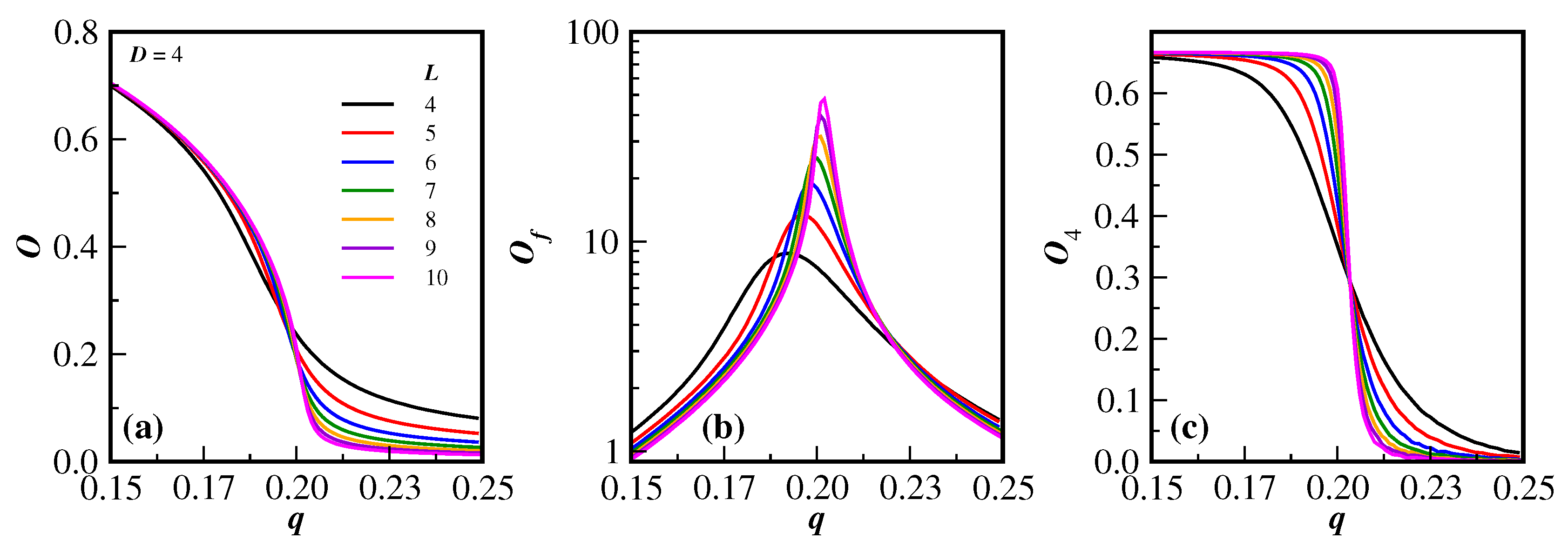
Figure 2.
(color online) Fourth-order Binder cumulant of the order parameter , as a function of the disorder parameter q, for several finite lattices of size L is shown in (a) for , in (c) for and in (e) for (the corresponding insets are an amplified view of the cumulant crossings close to the critical noise probability). The lines in the left panels are just a guide to the eyes. The right panels (b), (d) and (e) are the ln-ln plots of the cumulant derivative with respect to q as a function of the lattice size L for each dimension D. In these cases, the full lines are linear fits to the data. The inset in the right panels illustrates the behavior of as function of , with coming from the previous fits. The full lines are fits with logarithm finite-size corrections (in (b) a linear fit is also given by the dashed line).
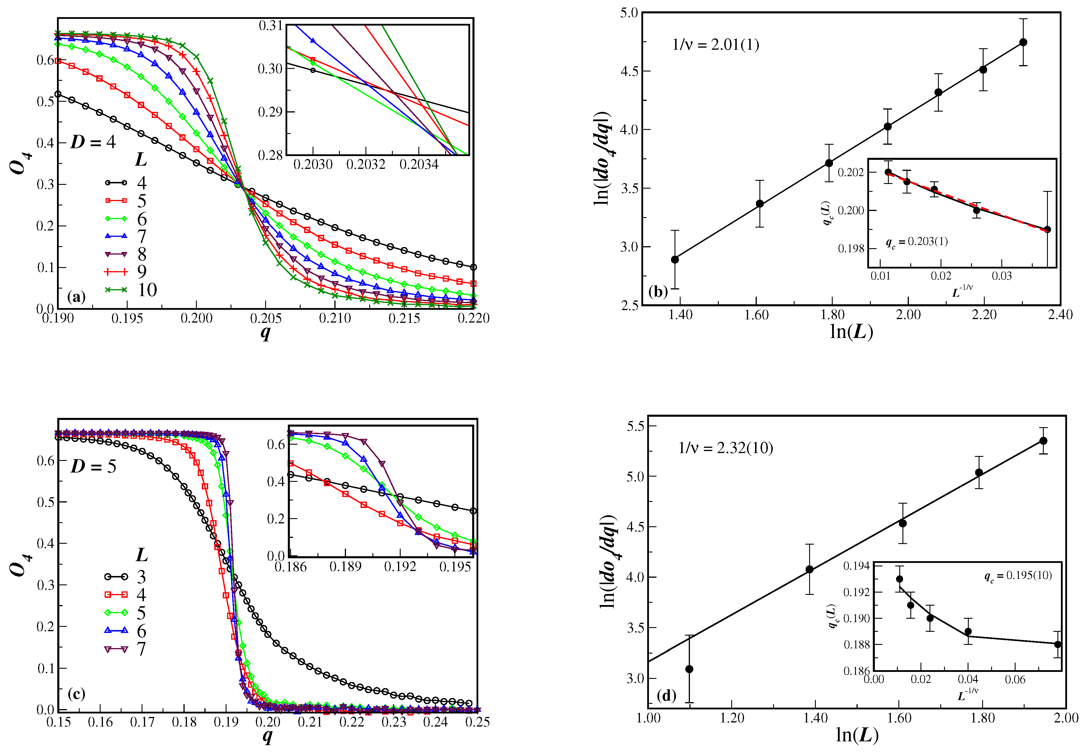
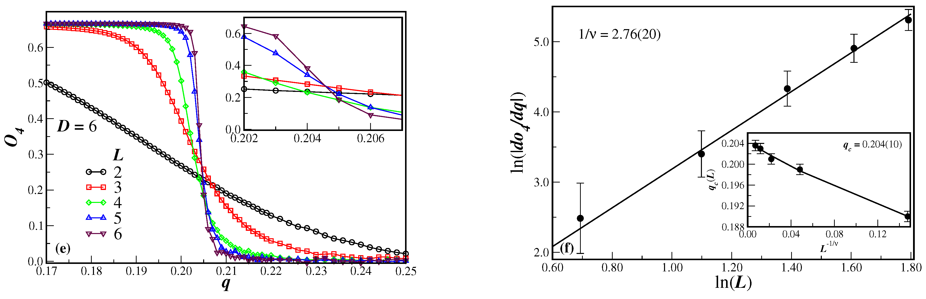
Figure 3.
(Color on-line). Ln-ln plots of as a function of lattice size L for in (a), in (b) and in (c). The function is, from top to bottom in each panel: the susceptibility of the average opinion at the estimated , ; the maximum value of the susceptibility at , ; and the average opinion at the estimated critical disorder, . The full lines are best linear fits according to Eqs. (9) and (10), with the corresponding slopes being the critical exponent ratios and , respectively. The legends convey the obtained values of the exponent ratios for each dimension D. In all cases, the error bar estimates are smaller than the symbol sizes
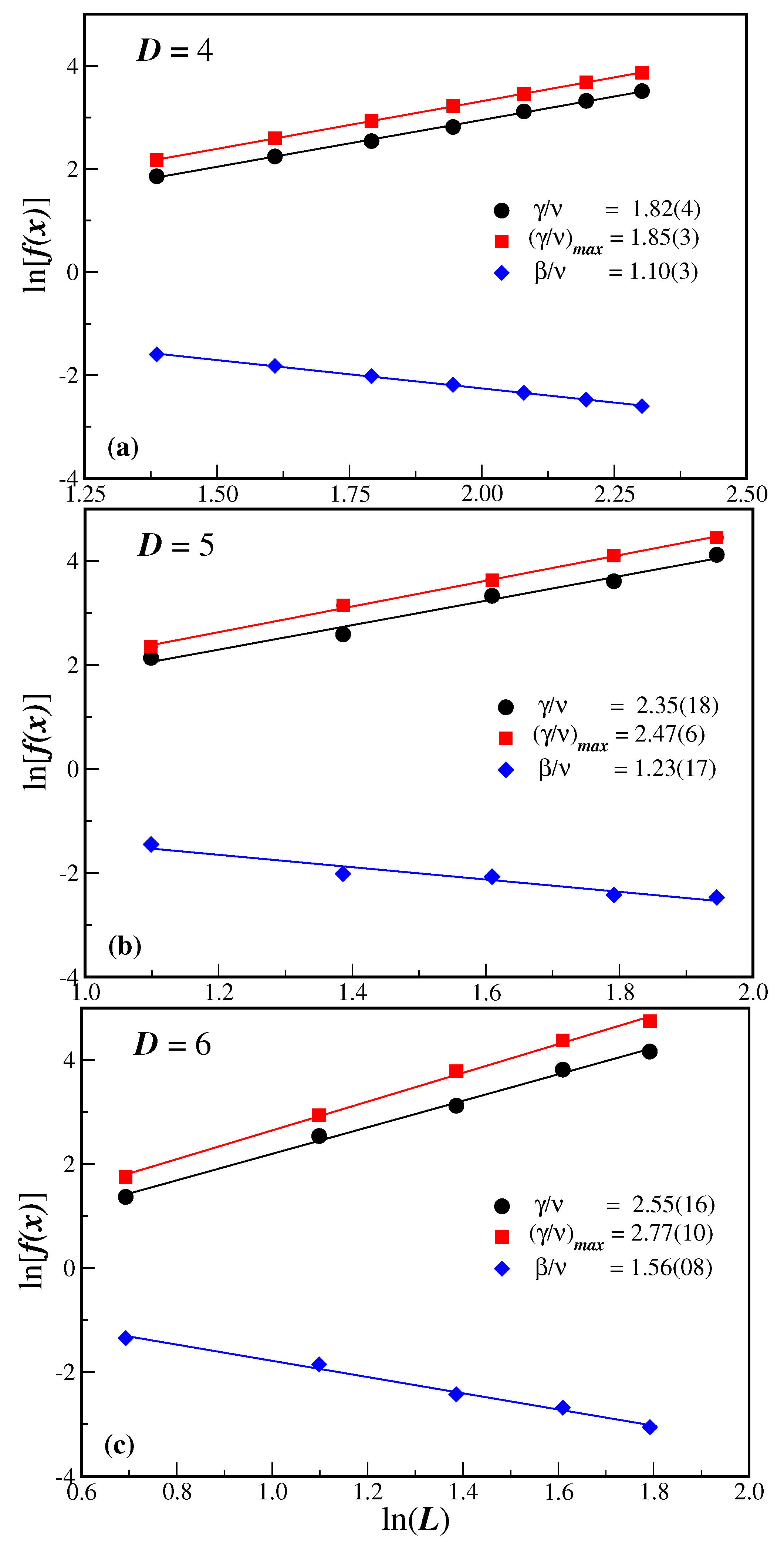
Figure 4.
(color online) Position of the maximum value of the fluctuation of the order parameter as a function of lattice size for different dimension D (given in the legend). The full lines are fits according to Eq. (14) with the extrapolated values of also given in the legend. The dashed line is an extra linear fit to the data only for .
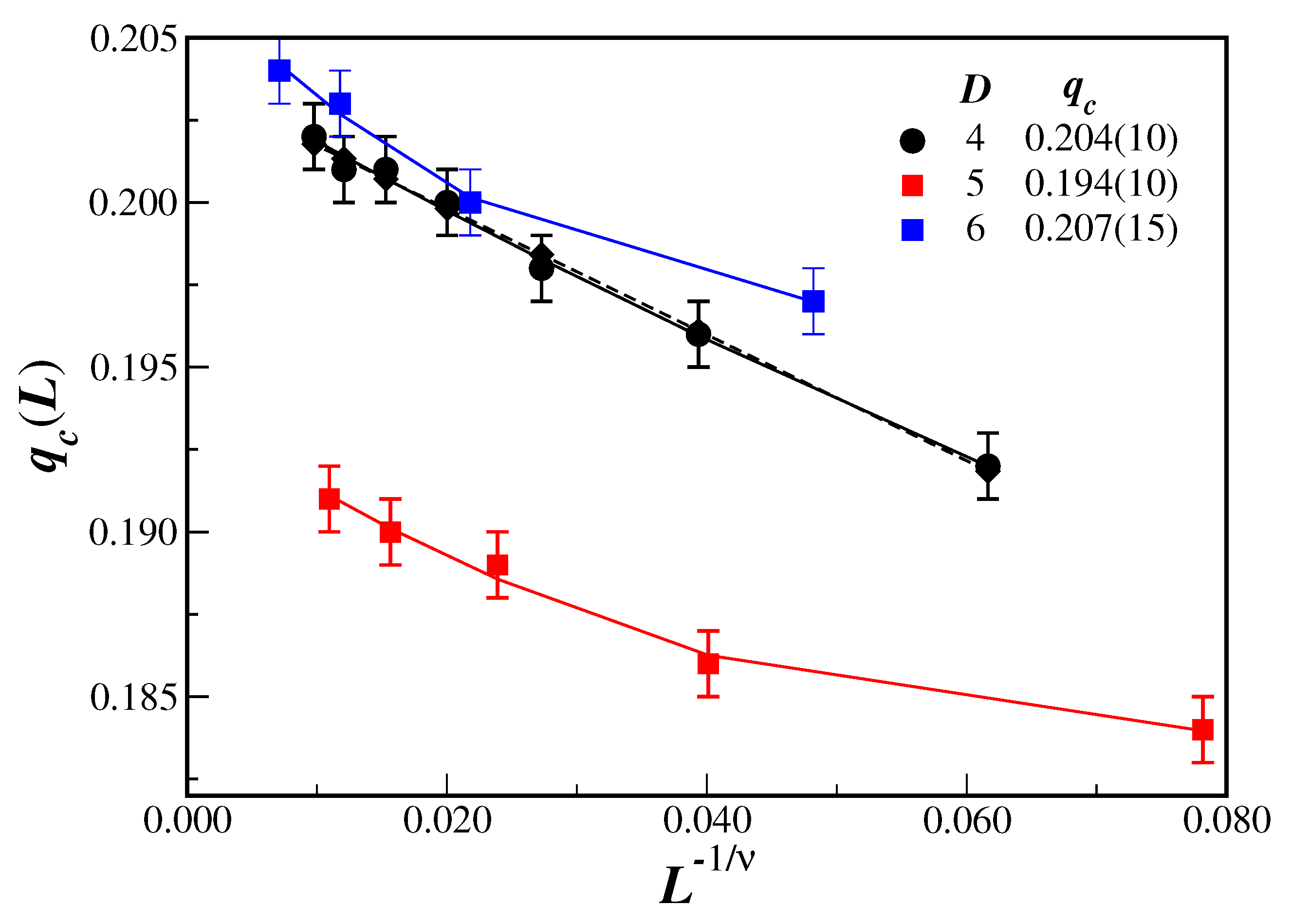
Figure 5.
(color online) The corresponding data collapse of the quantities displayed in Figure 1 using the finite-size scaling relations (9), (10), and (13) and combined with numerical data in Table 1, are given in panels (d), (e) and (f). The legends in the left panels also apply to the two right panels.
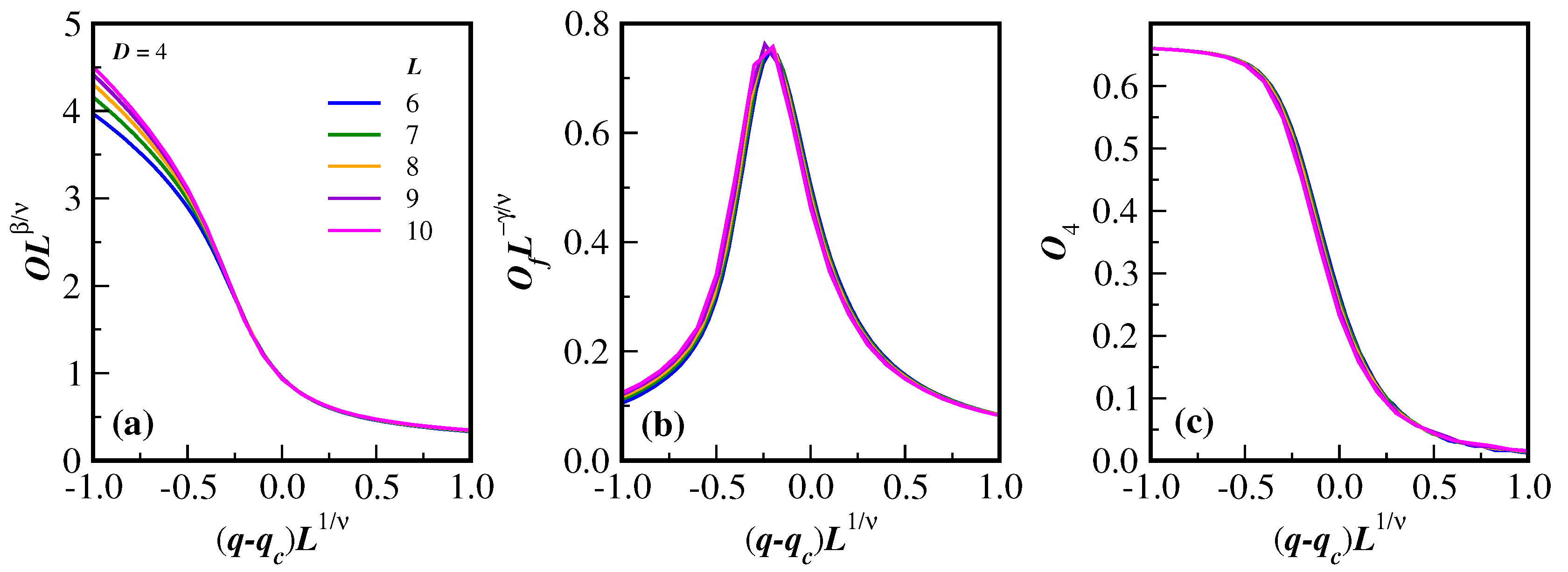

Table 1.
Critical noise probability and respective critical exponent ratios , and of the BChS model on SNs of different dimension D. The results obtained for , 2 and 3 on the same networks come from Refs. [18,19]. The exponent ratio are the results from the maximum value of the order parameter susceptibility. The last column gives the hyperscaling relation. Error bars are statistical only.
| D | |||||||
|---|---|---|---|---|---|---|---|
| 1 | 1.92(10) | ||||||
| 2 | 2.17(5) | ||||||
| 3 | 1.84(15) | ||||||
| 4 | 1.99(8) | ||||||
| 5 | 2.16(5) | ||||||
| 6 | 2.17(10) |
Disclaimer/Publisher’s Note: The statements, opinions and data contained in all publications are solely those of the individual author(s) and contributor(s) and not of MDPI and/or the editor(s). MDPI and/or the editor(s) disclaim responsibility for any injury to people or property resulting from any ideas, methods, instructions or products referred to in the content. |
© 2025 by the authors. Licensee MDPI, Basel, Switzerland. This article is an open access article distributed under the terms and conditions of the Creative Commons Attribution (CC BY) license (http://creativecommons.org/licenses/by/4.0/).
Copyright: This open access article is published under a Creative Commons CC BY 4.0 license, which permit the free download, distribution, and reuse, provided that the author and preprint are cited in any reuse.


