Submitted:
06 August 2025
Posted:
06 August 2025
Read the latest preprint version here
Abstract
A correspondence between fault damage mechanics and critical point models of seismic activation is presented, and a method of testing the correspondence against seismic measurements is outlined.
Keywords:
seismic activation
; fault dynamics
; statistical physics
; signal processing
1. Introduction
An increase in the number of intermediate sized earthquakes of moment magnitude in a seismic region preceding the occurrence of a mainshock event, referred to as seismic activation, has been documented by various researchers [5]. For example, seismic activation was observed in a geographic region spanning for a period of time between 1991 and 1999 preceding the magnitude 7.6 Chi-Chi earthquake [9]. Figure 1 shows a schematic plot of the cumulative distribution of earthquakes of different magnitudes in a seismic activation region in two different time intervals of equal duration preceding occurrence of a major () earthquake at time . In this figure, is a real time parameter, and is the characteristic time of major earthquake recurrence assuming an earthquake of similar magnitude occurred in the same region at [21,30]. Importantly, the cumulative distribution of earthquake magnitudes in a time interval of fixed width increasingly deviates away from a Gutenberg-Richter distribution as the end of the time interval approaches .
As a means of predicting the time at which a mainshock event preceded by seismic activation occurs, it has been hypothesized that the average seismic moment of earthquakes occuring in time intervals preceding a mainshock event obeys an inverse power of time to failure law:
and that the cumulative Benioff strain , defined as:
where is the seismic moment of the earthquake in the region starting from a time preceding the mainshock event, and is the number of earthquakes occurring in the region up to time , satisfies [28]:
The exponent selection of in Equation (2) is not necessary to derive formula (3) with a different arithmetic relation between and , but appears to have been selected by previous researchers based on Benioff’s finding that the elastic rebound of an earthquake is proportional to the square root of its seismic moment. When formula (3) is fit to real seismic data, a typical value of is [5,29]. Notably, validity of Equation (1) has been questioned by some researchers who claim measurements of seismic activation can be explained in terms of mainshock event foreshock occurrence without acceleration of seismic release [14,32].
A model of seismic activation based on fault damage mechanics (FDM) has been used to derive Equation (3) with a value [3]. In this derivation, the seismic activation region is modeled as a 1D fault consisting of perfectly plastic material whose effective shear modulus decreases to 0 as . The result is obtained from an effective shear modulus evolution equation based on non-equilibrium thermodynamic considerations [2].
In addition to the FDM model of seismic activation, a statistical mechanics model of seismic activation known as the Critical Point (CP) model has been put forth to derive Equation (3) with a value [21]. In this derivation, the inverse power of remaining time to failure law:
is asserted based on identifying the mean rupture length of earthquakes occuring at time with the correlation length of a statistical mechanical system described by a time dependent Ginzburg-Landau equation, whereby:
which implies relation (4) assuming [22]. Table 1 shows typical fault material displacements and rupture lengths for earthquakes of different moment magnitudes.
Importantly, previous work on the CP model has not explained why it is physically reasonable to describe seismic activation earthquake occurrence statistics with thermal equilibrium statistical mechanics formalism. Therefore, the first objective of this article is to conjecture how FDM and CP models of seismic activation are in correspondence with each other and provide computational evidence for this conjecture. The second objective is to outline how the conjectured correspondence can be tested against seismic measurements.
To meet these objectives, two different pre-existing seismicity models are developed: the earthquake cascade model and the renormalization group theory of earthquakes [25,27]. The earthquake cascade model provides an explanation for earthquake occurrence statistics in windows of time preceding a mainshock event in terms of the statistics of metastable clusters of fault material of different size within the activation region that can join together to create larger clusters or undergo slip events to initiate earthquakes. The renormalization group theory of earthquakes explains how the formalism of equilibrium statistical mechanics accounts for time scaling of cumulative Benioff strain during seismic activation in terms of statistical mechanics critical scaling theory, without explicitly identifying the relevant statistical mechanical system. For the purposes of this article, the earthquake cascade model is developed into a random matrix model of the seismic activation region stiffness matrix, and the renormalization group theory of earthquakes is developed into a description of the time evolution of the random stiffness matrix model. In so doing, correspondence between FDM and CP seismic activation models is clarified, because the random stiffness matrix is an FDM description of fault material elastoplastic deformation, and time evolution of the random stiffness matrix is specified by statistical mechanics critical scaling theory. The conjectured correspondence between FDM and CP seismic activation models is of applied science interest because it implies a finite dimensional nonlinear dynamical system governs real time evolution of the activation region elastic model before mainshock event occurrence, and this implication can be tested against seismic measurements.
The outline of the article is as follows. Section 2 introduces the earthquake cascade model with reference to laboratory studies of rock fracture, and explains how this model is related to a random matrix model of the seismic activation region stiffness matrix. Section 3 provides a computation of metastable cluster size distribution in terms of random matrix eigenvalue statistics, conjectures how time evolution of the random stiffness matrix model is described by 2D statistical mechanics critical scaling theory, and outlines how this conjecture can be tested against seismic measurements. Section 4 comments on application of seismic activation statistical physics models.
2. Materials and Methods
2.1. Earthquake Cascade Model
It has been observed that fracture processes occurring within the Earth preceding unstable slip along a mainshock fault are analogous to fracture processes occurring in triaxially loaded rock samples preceding sample failure [19]. Triaxial test results indicate 4 stages of rock deformation leading to sample failure [10]:
- crack closure
- elastic deformation
- stable microcrack growth and extension
- unstable crack extension
Triaxial loading of sandstone samples with recording of acoustic emissions has further indicated that before unstable crack extension occurs, microcracks nucleate into clusters along faults where unstable cracks later propagate, in a process called shear localization [11]. These clusters are metastable in that they gradually grow in size before unstable crack extension occurs rapidly, and are the laboratory analog of clusters of metastable earthquake fault material whose size distribution is quantified by the earthquake cascade model.
The earthquake cascade model describes earthquake occurrence along a 2D earthquake fault. It defines as the number of metastable clusters of fault material of area at time , where a metastable cluster is defined as the region over which an earthquake slip propagates after initiation, and provides time evolution equations for these numbers based on cluster joining and earthquake slip initiation rates. Depending on selection of these rates, different earthquake occurrence statistics are output by the model. For example, at sufficiently low rates of earthquake occurrence, time invariant metastable cluster size statistics are:
for some constant , whereby:
and:
Under the assumption earthquake occurrence rate is proportional to metastable cluster area, Equation (8) specifies a Gutenberg-Richter scaling relation between frequency of earthquake occurrence and earthquake rupture area with b-value . To explain this statement, note that if is the number of earthquakes of moment magnitude greater than or equal to M occurring during the time interval , the Gutenberg-Richter law implies:
which using the seismic moment-magnitude relation:
and corner frequency scaling relation:
implies the frequency of earthquakes with corner frequency and rupture area proportional to satisfies:
To develop the earthquake cascade model to account for a continuum of possible metastable cluster sizes, the approach presented here is to modify a stochastic process model of landslide occurrence to model earthquake occurrence. Importantly, the details of the landslide model depend on whether the landslide is in a condition of secondary or tertiary creep, so its modification to describing seismicity depends on whether cumulative Benioff strain is increasing at a constant rate or accelerating.
2.2. FDM Random Matrix Model
A scalar Kesten process is a stochastic process:
where k is a discrete time index, , and and are identical and independently distributed random variables. This process has been used to model sequences of landslide velocity measurements during secondary creep by assuming and are log-normally distributed with , in which case the sequence of velocities are distributed according to an inverse gamma distribution satisfying:
for some constant for sufficiently large velocities v [16].
In modifying process (13) to model earthquake occurrence during periods of non-accelerating cumulative Benioff strain, it is logical that the seismic stochastic process reflect classical mechanical time evolution of the seismic region, and output a random variable whose distribution accounts for the Gutenberg-Richter law. To this end, rather than describing time evolution of a single landslide velocity, it is suggested that the seismic stochastic process describe the time evolution of velocities of slow strain waves passing through the seismic activation region, and thereby also describe time evolution of metastable clusters of fault material formed by coherent motion of two or more slow strain waves. In 1 spatial dimension, slow strain waves propagating along crustal faults have been analyzed as kink solutions to a sine-Gordon equation with solitary wave velocity profiles:
where the wave velocity V can range from a velocity of seismicity migration ( to m/s) to an earthquake rupture velocity ( to m/s), and is the thickness of fault material [7]. In terms of inverse scattering theory of the sine-Gordon equation, the velocity and width of kink solutions satisfy:
where is the earthquake rupture velocity, is a characteristic fault material thickness, and is a complex number that is real when the frequency is a pure imaginary number identifying a 1D bound state of the sine-Gordon scattering problem [1].
The inverse scattering description of solitary waves in 1 spatial dimension can be generalized to 3 spatial dimensions using finite element analysis. Specifically, suppose the seismic activation region is contained within a hemisphere centered on the Earth’s surface, and subsurface material within the hemisphere is meshed with finitely many structural elements. A nodal displacement vector perturbing a finite strain elastoplastic deformation of material within the hemisphere at time then satisfies an equation:
where , , and are the frequency dependent finite element mass, damping, and tangent stiffness matrices at time , and is the vector of external forces acting on the nodes [4]. Assuming the external force is 0, the condition:
may specify finitely many pure imaginary eigenvalues and associated eigenvectors characterizing bound states in 3 spatial dimensions.
When the stiffness and damping matrices and external forcing vector can be approximated as being independent of , Equation (18) can be written:
which in absence of external forcing, Equation (20) implies is an eigenvalue of the matrix:
Therefore, if there exists an operator forming a Lax pair with :
the bound state spectrum (i.e. real eigenvalues) of remains constant as increases, while the eigenvectors of depend on , with the equation:
specifying this time dependence.
To pass from a deterministic to stochastic description of seismic activation region elastodynamics, differential Equation (22) may be modified to a discrete time stochastic process that outputs a sample path for , now regarded as belonging to an ensemble of random matrices. From this point of view, the bound state eigenvalues of the operator , indexed , may be distributed according to a random matrix eigenvalue distribution:
where is the Vandermonde determinant of the bound state eigenvalues, is a confining potential of the bound state eigenvalues in 1 spatial dimension, and is henceforth referred to as a damage parameter [12]. Physically, in analogy to dependence of kink velocity on bound state eigenvalue expressed by Equation (16), distribution (24) may be interpreted as an indirect description of the distribution of slow strain wave velocities in the seismic region.
In a seismic region with non-accelerating cumulative Benioff strain, random matrix model (24) may describe the slow strain wave velocity distribution with a constant value of . However, in a seismic activation region, it is necessary to allow for dependence of the damage parameter and function to describe the distribution of bound state eigenvalues solving nonlinear eigenvalue problem (19). The renormalization group theory of earthquakes suggests this time dependence can be precisely quantified using statistical mechanics critical scaling theory. Requiring that the critical scaling theory describe statistics of solutions to a nonlinear eigenvalue problem suggests the relevant statistical mechanical system is 2D, and requiring that the bound state eigenvalue statistics account for the Gutenberg-Richter law suggests the relevant statistical mechanical system contains vortex-antivortex dipole lengths R distributed according to an inverse power law at thermal equilibrium.
3. Results
3.1. FDM Random Matrix Eigenvalue Computation
3.1.1. 2D Critical Scaling Theory
In addition to identifying bound state eigenvalues, solutions to Equation (19) also identify scattering resonances of the seismic activation region. These resonant eigenvalues are inherently complex, and with selection of stiffness and damping matrices from a random matrix ensemble, are distributed randomly in the complex plane. For this reason, it is conjectured that a 2D statistical mechanical field theory describes the distribution of resonant eigenvalues in the complex plane.
Furthermore, depending on whether incoming or outgoing boundary conditions are specified on the hemisphere , resonant eigenvalues may be labeled as positive or negative. This suggests the 2D statistical mechanical system is a 2D Dyson gas, whereby the statistics of bound state eigenvalues describes the size distribution of positive-negative dipoles in the complex plane. From this point of view, a correspondence between metastable cluster and dipole size distribution statistics is established, since a Gutenberg-Richter distribution of earthquake corner frequencies, is:
where , and the distribution of dipole sizes satisfies a power law [26]:
In absence of further development, the renormalization group theory of earthquaes postulates the existence of -dependent statistical mechanical systems related by renormalization group transformation, whereby the cumulative Benioff strain at time equates to the expectation value of a statistical mechanical observable C for which:
is infinite for some finite positive integer k at a sequence of values approaching , which locates a statistical mechanical critical point [13,25]. With stochastic modeling of the seismic activation region presented in this article, the renormalization group theory of earthquakes is developed by conjecturing that the renormalized statistical mechanical system is a 2D Dyson gas, and the renormalization group fixed point is a critical point of the KT phase transition.
A more precise characterization of the 2D statistical mechanical system can be conjectured by noting that if Equation (20) is altered to include dependence of seismic activation region stiffness and damping it becomes:
when . This equation implies the matrix:
has determinant 0 at . Viewed as a dependent relation between and , the condition:
can be ensemble averaged over the dependent distribution of random stiffness and damping matrices to obtain an average relation between and , hereby conjectured to be a Riemann surface spectral curve. From this point of view, if the genus g of the average spectral curve remains constant as , the renormalization group flow of the 2D statistical mechanical system may be identifiable as the motion of a point in a Siegel moduli space [8]. For sake of specificity, it is further conjectured that this 2D statistical mechanical model of accelerating seismic release has bosonic fields, where is the number of bound state eigenvalues characterizing the metastable cluster of fault material initiating the mainshock event.
3.2. Geophysical Test
From a geophysical testing point of view, if it is true that the real time evolution of a seismic activation region elastic model preceding a mainshock can be quantified in terms of a 2D statistical mechanics model renormalization group flow, expressible as a nonlinear dynamical system of finite phase space dimension, a geophysical signal processing technique known as singular spectrum analysis should apply to determine this phase space dimension [6]. Therefore, it is conjectured that measurements of relative changes in seismic wave velocity between pairs of seismic stations in a seismic region obtained at regular time intervals during a seismic activation series can be input to a time domain multichannel singular spectrum analysis algorithm to output a finite phase space dimension [17]. More specifically, the number of channels of the algorithm equates to the number of station pairs, and the number of singular values output by the algorithm in different time windows preceding a mainshock event counts the number of unstable stress/strain modes contributing to mainshock rupture nucleation. With reference to previous geophysical application of singular spectrum analysis, performed in the frequency domain, the signal processing algorithm suggested here is different in that it should be carried out in the time domain rather than the frequency domain [24].
4. Discussion
Previous work has identified predicting the time of occurrence of mainshock events as an application of statistical physics models of seismic activation, but this application has not yet been realized [5]. In more recent times, the artificial intelligence algorithm QuakeGPT has been developed for the purpose of forecasting earthquake occurrence, using seismic event record training data created with a stochastic simulator [23]. Therefore, a practical application of statistical mechanics models of seismic activation may be to be improve stochastic simulation of seismic event records for use in earthquake forecasting technology, acknowledging that rigorous tests of model validity against real seismic data must be passed before achieving this objective can be considered a realistic possibility.
In conclusion, work towards improving current earthquake early warning systems can proceed in two directions. Firstly, work can be done to determine whether or not observed changes of the Earth’s elastic velocity model preceding mainshock events can be processed to extract an integer identifiable as the phase space dimension of a nonlinear dynamical system. Secondly, theoretical work can be done to elaborate upon the statistical mechanics model of seismic activation presented in this article to determine other tests of its scientific validity and potential for practical application.
Funding
This research received no external funding.
Institutional Review Board Statement
Not applicable.
Informed Consent Statement
Not applicable.
Acknowledgments
Thanks to my family for their support throughout completion of this research. Thanks to Girish Nivarti, Evans Boney, and Professor Richard Froese for their willingness to entertain communication regarding the content of the article.
Conflicts of Interest
The authors declare no conflicts of interest.
Abbreviations
The following abbreviations are used in this manuscript:
| MDPI | Multidisciplinary Digital Publishing Institute |
| DOAJ | Directory of open access journals |
| TLA | Three letter acronym |
| LD | Linear dichroism |
References
- Aktosun T, Demontis F, Van der Mee C. Exact solutions to the sine-Gordon equation. Journal of Mathematical Physics 2010, 51, 12.
- Ben-Zion, Y. Collective behavior of earthquakes and faults: Continuum-discrete transitions, progressive evolutionary changes, and different dynamic regimes. Reviews of Geophysics 2008, 46, 4. [Google Scholar] [CrossRef]
- Ben-Zion Y, Lyakhovsky V. Accelerated seismic release and related aspects of seismicity patterns on earthquake faults. Earthquake processes: Physical modelling, numerical simulation and data analysis Part II 2002, 2385–2412.
- Bindel, DS. Structured and parameter-dependent eigensolvers for simulation-based design of resonant MEMS. Doctoral dissertation. University of California, Berkeley. 2006.
- Bowman D, Ouillon G, Sammis C, Sornette A, Sornette D. An observational test of the critical earthquake concept. Journal of Geophysical Research: Solid Earth, 2435.
- Broomhead DS, King GP. Extracting qualitative dynamics from experimental data. Physica D: Nonlinear Phenomena.
- Bykov, VG. Solitary waves on a crustal fault. Volcanology and Seismology 2001, 22(6), 651–661. [Google Scholar]
- Carpentier, D. Renormalization of modular invariant Coulomb gas and sine-Gordon theories, and the quantum Hall flow diagram. Journal of Physics A: Mathematical and General 1999, 32, 3865. [Google Scholar] [CrossRef]
- Chen, CC. Accelerating seismicity of moderate-size earthquakes before the 1999 Chi-Chi, Taiwan, earthquake: Testing time-prediction of the self-organizing spinodal model of earthquakes. Geophysical Journal International 2003, 155(1), F1–F5. [Google Scholar] [CrossRef]
- Dou L, Cai W, Cao A, Guo W. Comprehensive early warning of rock burst utilizing microseismic multi-parameter indices. International Journal of Mining Science and Technology 2018, 28, 767–747. [CrossRef]
- Fortin J, Stanchits S, Dresen G, Gueguen Y. Acoustic emissions monitoring during inelastic deformation of porous sandstone: comparison of three modes of deformation. Pure and Applied Geophysics 2009, 166, 823–841. [CrossRef]
- Gautié T, Bouchaud JP, Le Doussal P. Matrix Kesten recursion, inverse-Wishart ensemble and fermions in a Morse potential. Journal of Physics A: Mathematical and Theoretical 2021, 54, 255201. [CrossRef]
- Goldenfeld, N. Continuous Symmetry. In Lectures on phase transitions and the renormalization group; CRC Press, 2018; pp. 335–350.
- Hardebeck JL, Felzer KR, Michael AJ. Improved tests reveal that the accelerating moment release hypothesis is statistically insignificant. J. Geophys. Res. 2008, 113. [Google Scholar]
- Ito R, Kaneko Y. Physical mechanism for a temporal decrease of the Gutenberg-Richter b-Value prior to a large earthquake. Journal of Geophysical Research: Solid Earth 2023, 128, 12.
- Lei Q, Sornette D. A stochastic dynamical model of slope creep and failure. Geophysical Research Letters 2023, 50, 11.
- Merrill RJ, Bostock MG, Peacock SM, Chapman DS. Optimal multichannel stretch factors for estimating changes in seismic velocity: Application to the 2012 Mw 7.8 Haida Gwaii earthquake. Bulletin of the Seismological Society of America 2023, 113, 1077–1090. [CrossRef]
- Peskin, ME. An introduction to quantum field theory. CRC press. 2018.
- Reches, ZE. Mechanisms of slip nucleation during earthquakes. Earth and Planetary Science Letters 1999, 170(4), 475–486. [Google Scholar] [CrossRef]
- Riccobelli D, Ciarletta P, Vitale G, Maurini C, Truskinovsky L. Elastic instability behind brittle fracture. Physical Review Letters 2024, 132, 24.
- Rundle JB, Klein W, Turcotte DL, Malamud BD. Precursory seismic activation and critical-point phenomena. Microscopic and Macroscopic Simulation: Towards Predictive Modelling of the Earthquake Process 2001, 2165–2182.
- Rundle JB, Turcotte DL, Shcherbakov R, Klein W, Sammis C. Statistical physics approach to understanding the multiscale dynamics of earthquake fault systems. Reviews of Geophysics 2003, 41, 4.
- Rundle JB, Fox G, Donnellan A, Ludwig IG. Nowcasting earthquakes with QuakeGPT: Methods and first results. In Scientific Investigation of Continental Earthquakes and Relevant Studies; Springer Nature, Singapore, 2025.
- Sacchi, M. FX singular spectrum analysis. In Cspg Cseg Cwls Convention, 392–395.
- Saleur H, Sammis C, Sornette D. Renormalization group theory of earthquakes. Nonlinear Processes in Geophysics 1996, 3(2), 102–109. [Google Scholar] [CrossRef]
- Tattersall RJ, Baggaley AW, Billam TP. Out-of-equilibrium behavior of quantum vortices: A comparison of point vortex dynamics and Fokker-Planck evolution. Physical Review A 2025, 112, 013313. [CrossRef]
- Turcotte DL, Malamud BD. Earthquakes as a complex system. International Geophysics Academic Press.. 2002, 81.
- Tzanis A, Vallianatos F, Makropoulos K. Seismic and electrical precursors to the 17-1-1983, M7 Kefallinia earthquake, Greece: Signatures of a SOC system. Physics and Chemistry of the Earth, Part A: Solid Earth and Geodesy 2000, 25, 281–287. [CrossRef]
- Vallianatos F, Chatzopoulos G. A complexity view into the physics of the accelerating seismic release hypothesis: Theoretical principles. Entropy 2018, 20, 754. [CrossRef]
- Vallianatos F, Sammonds P. Evidence of non-extensive statistical physics of the lithospheric instability approaching the 2004 Sumatran–Andaman and 2011 Honshu mega-earthquakes. Tectonophysics 2004, 590, 52–58.
- Xue L, Belytschko T. Fast methods for determining instabilities of elastic–plastic damage models through closed-form expressions. International Journal for Numerical Methods in Engineering 2010, 84, 1490–1518. [CrossRef]
- Zhou S, Johnston S, Robinson R, Vere-Jones D. Tests of the precursory accelerating moment release model using a synthetic seismicity model for Wellington, New Zealand. J. Geophys. Res.2006,111.
Figure 1.
Plot of the cumulative distribution of earthquakes of different moment magnitudes in a seismic activation region in two different time intervals of equal width preceding occurrence of a major earthquake at [21,30].
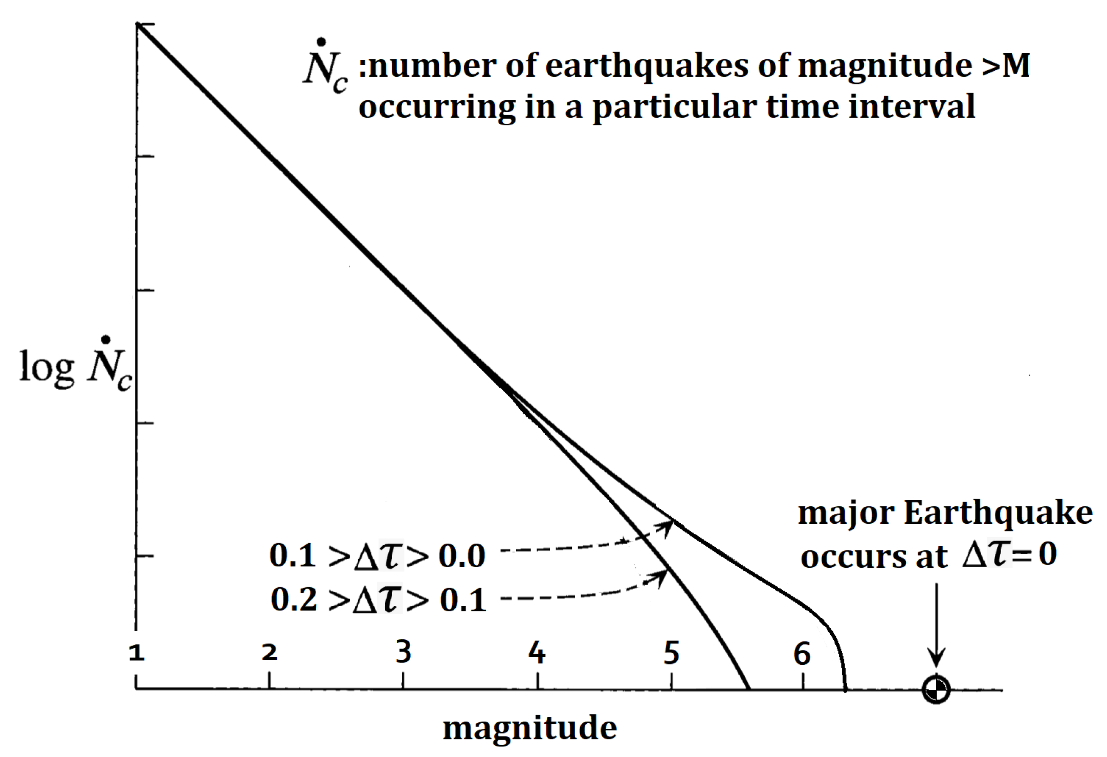

Table 1.
Approximate relation between earthquake magnitude, fault material displacement, and fault rupture length.
Table 1.
Approximate relation between earthquake magnitude, fault material displacement, and fault rupture length.
| Moment Magnitude | Average Fault Material Displacement (m) | Fault Rupture Length (km) |
|---|---|---|
| 4 | 0.05 | 1 |
| 5 | 0.15 | 3 |
| 6 | 0.5 | 10 |
| 7 | 1.5 | 30 |
| 8 | 5 | 100 |
Disclaimer/Publisher’s Note: The statements, opinions and data contained in all publications are solely those of the individual author(s) and contributor(s) and not of MDPI and/or the editor(s). MDPI and/or the editor(s) disclaim responsibility for any injury to people or property resulting from any ideas, methods, instructions or products referred to in the content. |
© 2025 by the authors. Licensee MDPI, Basel, Switzerland. This article is an open access article distributed under the terms and conditions of the Creative Commons Attribution (CC BY) license (http://creativecommons.org/licenses/by/4.0/).
Copyright: This open access article is published under a Creative Commons CC BY 4.0 license, which permit the free download, distribution, and reuse, provided that the author and preprint are cited in any reuse.


