
Submitted:
24 March 2023
Posted:
27 March 2023
You are already at the latest version
Abstract
We propose a new statistical analysis of the Acoustic Emissions (AE) produced in a series of triaxial deformation experiments leading to fractures and failure of two different rocks, namely, Darley Dale Sandstone (DDS) and AG Granite (AG). By means of q-statistical formalism, we are able to characterize the pre-failure processes in both types of rocks. In particular, we study AE inter-event time and AE inter-event distance distributions. Both of them can be reproduced with q-exponential curves, showing universal features which are observed here for the first time and could be important in order to understand more in detail rock fractures dynamics.
Keywords:
Acoustic emissions
; q-statistics
; rocks fractures
1. Introduction and Motivation
The analysis of the Acoustic Emissions (AE) in materials under deformation in laboratory experiments, is a very important technique for understanding the damage accumulation and failure modes [1,2,3,4,5,6,7].
AE are high frequency elastic waves due to micromechanical damage induced by the micro-cracking. These emissions therefore represent indicators of deformation and fracturing processes occurring within a tested specimen and allow to monitor cracking formation, growth and propagation. The detection of the AE can therefore allow both to understand how the damage accumulates and develops within the material, and to monitor the final rupture. This information could be very useful in geophysics, for the interpretation of field scale seismic signals and the understanding of earthquakes precursors. Furthermore, a deep insight in the cracking propagation in the considered rocks can also be very important in civil engineering, for monitoring the integrity of bridges and buildings and develop strategies for safe design of tunnels.
From the seismological point of view AE obey, as earthquakes, to the Gutenberg-Richter relationship between frequency and magnitude. Rock fracture and earthquake rupture are processes obeying similar statistics for source dimensions over more than eight orders of magnitude [8,9]. In order to link experimental detailed studies to geophysical signatures recorded at the field scale, controlled laboratory rock deformation experiments equipped with dense microseismic arrays for AE detection have become a routinely used tool [10,11,12]. Here, fault growth may be considered analogous to the field scale development of earthquake rupture generating acoustic emissions, which is a well-used analog to tectonic earthquakes due to the scale invariance of these processes [13,14,15]. Source mechanisms evolution with respect varying effective pressure can also be inferred from AE, allowing to determine the effect of the increasing lithostatic pressure on the fracturing mechanisms and failure mode [16].
In a civil engineering context, any project for the seismic design or monitoring of large structures needs to consider soil-structure interaction. The dynamic response of buildings or bridges, for example, is closely related to the mechanical behavior of the foundation soil. Other structures of great importance in civil engineering, whose behavior under seismic excitations is closely related to the nature of the surrounding rocks, are the tunnels. A reliable geological information is very important in seismic design of tunnels [17,18]. Excavation methods, dimensions and design parameters of a tunnel strictly depend on the type of rocks along its alignment. The mechanical information regarding soil and rocks are obtained by means of appropriate tests performed either in situ or from samples. In the case of tunnels, the surrounding rocks are subjected to distributed pressures which may vary in direction and intensity. When samples of rocks are extracted, it is therefore important to reproduce in 3D experimental tests the effects of the distributed confinement pressures. A reliable 3D laboratory test on soils and rocks, is the triaxial test which allows to evaluate the effect of confinement pressures on the failure load of the specimens [19,20,21,22].
In this paper we present a new analysis of the AE recorded during conventional triaxial deformation tests. In particular, our experimental setup allows recording AE generated during the loading by the crack initiation, propagation and growth leading eventually to macro-fractures formation and sample failure. In this context, the use of non-extensive q-statistics has recently proved to be particularly effective in capturing some universal features which emerge during the cracks propagation under loading [1,7]. In a previous paper, some of the authors of this paper investigated, by means of q-statistics, AE in uniaxial compression experiments on samples of Basalt and Concrete subjected to cyclic loading [5]. The aim of the present study is to apply a similar statistical analysis to AE obtained in triaxial compression tests in order to take into account the effect of the confining pressure on the AE release and assess the influence of increasing confining pressure, different deformation and failure mode on the AE statistical properties.
2. Experimental Setup and Data Analysis
The AE used in this work have been recorded during conventional triaxial deformation experiments on cylindrical 40mm x 100mm samples with an array of twelve 1MHz single-component Piezo-Electric Transducers for AE detection (REF). Triaxial compression tests have been performed at 5,10,20 and 40MPa on geologically and physically (i.e., fabric, porosity, grain size, and cementation) different lithologies such the Darley Dale Sandstone (DDS, porosity 14%) and Alzo Granite (AG, porosity < 1%). The AE data sets have been analysed in terms of source mechanisms time and spatial evolution before the rupture from some of the authors [16]. AE source mechanisms analysis has evidenced single fracture nucleation for AG and multiple fracture nucleation for DDS due to single or multiple competing dilatant and compactant regions. Fracture growth and propagation appears controlled by the different confinements, with increasing pressure controlling the time evolution and size of dilatant and compactant regions, eventually controlling cracks coalescence into macroscopic fractures [16].
In order to give representative insights on the AE time and amplitude distribution prior failure, we plot in Figure 1 the AE amplitude (a) and the AE Inter-event time (b) as function of time for two samples: AG at 40 MPa (top panel) and DDS at 20 MPa (bottom panel). The inter-event time is the time interval (in seconds) between two consecutive recordings AE(n) and AE(n − 1) and can be defined as:
where tAE(n) is the time at which the n-th AE event does occur and tAE(n−1) the time of the previous event.
The coupled analysis of AE amplitude and interevent times reveals that AG shows an abrupt increase at the end of the elastic phase, between 500 and 1000 seconds, then AE amplitude remains quite constant until failure (which happens at about 2800s) and, finally, it suddenly decreases during the stick-slip AE events occurring in the post-failure phase, with occasional AE clusters of higher amplitude driven by stress at the fault asperities; on the other hand, DDS presents a much more gradual AE amplitude increase from 500 to 1500 seconds, reaching steady values before failure (which happens at about 2400s), then a decrease driven by the post-failure stick-slip processes. This difference can be explained by the different deformation mechanisms acting on the different lithologies. In fact, at the end of each sequence, macroscopic structure forms. For AG, a single damage cycle of crack nucleation and growth is sufficient to propagate fractures and develop the planar localization leading to dynamic failure. Whilst in DDS it can take multiple cycles of nucleation for coalescence to take place due to interacting mechanisms induced by multiple fracture nucleation sites [16].
Thus, the DDS shows a much clear premonitory phase, or foreshock, before a critical damage threshold which would allow the coalescence into a larger scale deformation structure. For both the samples, failure is characterized by a peak in the AE interevent time, which suddenly appears after a sequence of very low values corresponding to the sequence of high amplitude events before rupture, corresponding to the transition from mm scale propagating microfractures to a fully developed cm scale fault zone.
In Table 1 we report, for each sample, the time tB at which the breakdown occurs, the total time tTOT of the experiment, the number N* of AE events before breakdown and the total number N of AE events present in the corresponding time series. In the following we will investigate if q-statistics can help in revealing different structures in these data sets for increasing levels of confinement.
AE Amplitudes
To start, let us look at the amplitude probability distributions of the acoustic emissions for our eight considered samples. Firstly, we explore these distributions by dividing each time series in four parts (time intervals):
- from the beginning to 30% tB
- from 30% tB to 70% tB
- from 70% tB to breakdown
- after breakdown.
Of course, the number of data included in each time interval could be even quite small, however such a procedure could bring out otherwise hidden details of the process leading to the rupture.
In Figure 2, the amplitude PDFs for AG (a) and DDS (b) samples, within each time interval and for each level of confinement, are plotted; the number of events included in each time interval is also reported in legenda.
We will not show distributions corresponding to time intervals with less than 50 AE events, due, of course, to the too poor statistics. We also anticipate that amplitude data for DDS at 5 MPa are not reliable, since they have been affected by a problem with the pre-amplifier gain during the experiment.
Comparing the various panels for the two types of lithologies, one immediately notices several features which reveal some kind of universal behavior:
- Events in the first time interval (within 30% tB) are always too few to give consistent distributions, regardless of the material;
- Distributions before and after failure are quite similar, again regardless of the material, with an initial sudden increase, a peak and a slow decrease for high amplitudes;
- Distributions after failure are more peaked for both AG and DDS.
Our approach identifies the background general behaviour driving the main mechanical phases of nucleation, growth, and coalescence of micro fractures into a macroscale fault zone, regardless the prevalence of a specific phase in a specific deformation stage driven by the different lithologies and effective pressures.
In Figure 3 the complete probability distributions for the whole time series of the different samples are reported both in Lin-Lin (a-b) and in Log-Lin (c-d) scale. It immediately appears that, for both the materials and all the confinements, all the curves collapse one onto the others (with the exception of DDS 5Mpa, which has been excluded for the reasons explained before) and in all cases show power-law tails which overlap one over the others. The shape of the Lin-Lin curves is similar to that found in Figure 2, but the plots in Log-Lin scale tell us that we are in presence of fat tails. This result confirms that the amplitude of the AE events is scale-invariant and does not depend on lithology and confinement. Both the distributions (c) and (d) can be well fitted with the following function, given by the product of a quadratic term and a q-exponential one (which, for q > 1, is a power law):
where = 7000, and = 1.19. The power-law which is introduced as a pre-factor of the q-exponential function is similar to the density of states which is present in the Planck law for the black-body radiation. Its origin here is possibly related to three-dimensional nearly isotropic stresses. Similar power-law pre-factors turn out to be necessary in diverse complex situations, such as the volume distributions in stock exchanges [23], distributions of transverse momenta of hadronic jets produced in proton-proton high-energy collisions at CERN/LHC [24], and COVID-19 peaks in the recent pandemics [25], among others.
AE Inter-Event Times
Let us now shift our attention to the AE inter-event times. In particular, we will study the complementary cumulative (decumulative) probability distributions of AE inter-event times for both the AG and DDS samples, adopting only data before breakdown.
To build the decumulative distribution P(> ) of the inter-event time series, one has to report, for each value of in the interval [0,1000], the fraction of inter-event times which are greater of that value. Therefore, in Log-Log scale, one could expect a curve starting from the unit for small values of , then, after a certain inflection point, gradually decreasing with some kind of peculiar behavior for high values of .
In similar experiments [1,5], these decumulative distributions exhibited clear power-law tails which can be framed in the context of the q-generalized thermostatistics: actually, in these cases simple q-exponential functions were able to well fit the obtained curves, thus unveiling the fractal or multifractal nature of the breakdown process. In the results presented here, as shown in Figure 4 for AG and in Figure 5 for DDS, we found something more complex than the expected power-law tails: in fact, the decumulative PDFs for both the type of analyzed materials seem to further change slope in correspondence of a second inflection point, whose time position decreases with increasing the confinement for DDS while seems to oscillate for AG. This new kind of behavior could be still described in the framework of q-thermostatistics, but adopting the following more general fitting function [26]:
It is composed by the sum of a first standard q-exponential function (with normalization factor , inverse temperature and entropic index ) and a second function containing (in addition to a normalization factor , an inverse temperature and an entropic index ) a further parameter which ensures that the total function monotonically vanishes for increasing inter-times with an appropriate behavior. See [27] for a similar crossover in the area-preserving dynamics of the standard map for intermediate values of the control parameter.
Looking to Figure 4 and Figure 5, it can be appreciated that function (2) is able to well fit all the PDFs, regardless of the material, provided that the following parameters are chosen:
In the previous Table 2 one can notice that, for any material and confinement, typically and . Moreover, in correspondence of the same amount of confinement, values of coincide for AG and DDS. A double q-exponential behavior, although kind of rare, occasionally emerges in complex systems. Such is the case for the nucleotide inter-distances in DNA sequences of Homo Sapiens [28].
AE Positions and Inter-event Distances
Finally, let us investigate about if the AE events are clustered in space. In order to do this, we first explore the behavior of their subsequent positions (expressed in meters), ordered in time before breakdown (with a blue scale of decreasing intensity) and projected on the three planes X-Y, X-Z and Y-Z, for both AG (Figure 6) and DDS (Figure 7) samples with the usual confinements.
Spatial distributions of AE show a higher clustering of events in AG, where fracturing occurs throughout localized planar fractures, while more scattered nucleation centers related to dilatant patches occur prior failure in DDS.
It is also useful to study the probability distribution of the AE inter-event distances (also expressed in meters), defined as the metric distance between the 3D spatial positions of two subsequent recorded AE events inside a given sample during an experiment:
In Figure 8 we plot the distributions of the inter-event distances before rupture obtained for both AG (top panel) and DDS (bottom panel) at the different levels of confinement. What we observe is a Planck-like distribution, with a maximum and an asymmetric tail, which can be well fitted by the following function:
where the values of the two fitting parameters (A = 4.8 107 and B = 132) are independent of the type of materials and of the confinement, thus revealing again some kind of universal behavior. On the other hand, it is well visible a single narrow peak around zero for some AG samples, in particular those with intermedium levels of confinement, a peak which is completely absent for DDS samples. This might be explained by the single fracture nucleation mechanisms observed for AG, implying high spatial clustering with respect to the multiple fracture nucleation mechanisms observed for DDS, due to multiple fracturing regions [16] and implying more diffused seismicity and a lower clustering.
To close this analysis, let us finally look at the decumulative distributions P(> ) of the inter-event distances before rupture, which are shown in Figure 9 for AG samples and in Figure 10 for DDS ones.
As for the inter-event times decumulative PDFs, also in this case it is possible to fit all the distributions with q-exponential functions, but in this case are enough single standard q-exponentials with inverse temperature and an entropic index q. Notice that, in analogy to what has been found in [29], values of the entropic indexes are all below 1, indicating not a power law behavior but revealing the presence of a cut-off in the distributions. Moreover, as shown in Table 3, in agreement with a further finding of [29], calling the first entropic index obtained for the inter-event time PDFs (see Table 2) and the entropic index just found for the inter-event distance, it can be noticed that the sum oscillates around 2 for all the samples, regardless of both material and confinement. This results is also similar to what has been observed in regional seismicity data from Japan and California and numerically verified using the two-dimensional Burridge-Knoppoff model [29].
In Figure 11 the entropic index is reported as function of . The figure clearly shows that the linear behavior holds quite well inside an error of 10% for almost all the samples.
The results of this study could be applied in different research fields, such as the collapse prediction of building materials and the interpretation of deformation mechanisms preceding and accompanying earthquake ruptures. Actually, regardless the deformation mechanisms, whether planar localization or dilatant patches developing at different effective pressures and lithologies, and driving the precursory phase before a critical damage threshold is reached, the macroscopic coalescence into a larger scale deformation structure and its seismic output would be controlled by the transition from mm scale fractures into a cm scale fault zone.
3. Conclusions
We investigated by means of q-formalism the Acoustic Emissions (AE) produced in a series of triaxial deformation experiments leading to fractures and failure of two different materials, namely, Darley Dale Sandstone (DDS) and AG Granite (AG). We have shown that pre-failure processes in both types of rocks, and in particular AE inter-event time and AE inter-event distance distributions, can be reproduced with q-exponential curves, showing universal features which are observed here for the first time. This characterization could be important in order to understand more in detail the processes of rock fractures dynamics and deformation mechanisms. The obtained results may have important applications both in civil engineering, in the analysis of soil-structure interaction, and in geophysics for the comprehension of seismic signals preceding and accompanying earthquakes.
References
- I. Stavrakas, D. Triantis, S.K. Kourkoulis, E.D. Pasiou, I. Dakanali, “Acoustic Emission Analysis of Cement Mortar Specimens During Three Point Bending Tests”, Latin Am. J. Solids Struc. 13, 2283 (2016). [CrossRef]
- I. Stavrakas, “Acoustic emissions and pressure stimulated currents experimental techniques used to verify Kaiser effect during compression tests of Dionysos marble”, Fracture and Structural Integrity 40, 32 (2017). [CrossRef]
- C. Stergiopoulos, I. Stavrakas, G. Hloupis, D. Triantis, F. Vallianatos, “Electrical and Acoustic Emissions in cement mortar beams subjected to mechanical loading up to fracture”, Eng. Failure Anal. 35, 454 (2013). [CrossRef]
- A. Kyriazopoulos, C. Anastasiadis, D. Triantis, F. Vallianatos, “Monitoring of Acoustic Emissions on three-point bending experiments in cement mortar beams in the light of non-extensive statistical physics”, in 1st Int. Conf. of the Greek Society of Exp. Mechanics of Materials, Athens, Greece, May 10–12, 2018, p. 77 (2018).
- A. Greco et al., “Acoustic emissions in compression of building materials: q-statistics enables the anticipation of the breakdown point”, Eur. Phys. J. Special Topics 229, 841–849 (2020). [CrossRef]
- D. Triantis, A. Loukidis, I. Stavrakas, E.D. Pasiou, S.K. Kourkoulis, “Attenuation of the Acoustic Activity in Cement Beams under Constant Bending Load Closely Approaching the Fracture Load”, Foundations 2, 590–606 (2022). [CrossRef]
- A. Loukidis, I. Stavrakas and D.Triantis, Non-Extensive Statistical Mechanics in Acoustic Emissions: Detection of Upcoming Fracture in Rock Materials, Appl. Sci. 13, 3249 (2023). [CrossRef]
- A. Zang, F.C. Wagner, S. Stanchits, G. Dresen, R. Andresen, and M.A. Haidekker, “Source analysis of acoustic emissions in AUE granite cores under symmetric and asymmetric compressive loads”, Geophysical Journal International, 135,1113–1130 (1998). [CrossRef]
- L. Burlini, S. Vinciguerra, G. Di Toro, G. De Natale, P. Meredith, J.P. Burg, “Seismicity preceding volcanic eruptions: new experimental insights”, Geology, 35(2),183-186 (2007). [CrossRef]
- P.M. Benson, B.D. Thompson, P.G. Meredith, S. Vinciguerra and R.P. Youn, “Imaging slow failure in triaxially deformed Etna basalt using 3D acoustic-emission location and X-ray computed tomography”, Geophysical Res. Lett., 34(3), L03303 (2007). [CrossRef]
- M. Fazio, P. Benson, S. Vinciguerra, “On the generation mechanisms of fluid-driven seismic signals related to volcano-tectonics”, Geophysical Research Letters, 44, 734-742 (2017). [CrossRef]
- D.A. Lockner, J. D. Byerlee, V. Kuksenko, A. Ponomarev, and A. Sidorin, “Quasi-static fault growth and shear fracture energy in granite”, Nature, 350, 39–42 (1991). [CrossRef]
- T.C. Hanks, “Small earthquakes, tectonic forces”, Science, 256, 1430–1432 (1992). [CrossRef]
- C.G. Hatton, I.G. Main & P.G. Meredith, “Non-universal scaling of fracture length and opening displacement”, Nature, v. 367, p. 160–162 (1994). [CrossRef]
- J. A. Hudson, B. L. N. Kennett, “Quantitative Seismology (two vols) K. Aki and P. G. Richards, W. H. Freeman, San Francisco 934 pp. $35.00 (£20.70 per volume)”, Geophysical Journal International, Volume 64, Issue 3, Pages 802–806 (1981). [CrossRef]
- T. King, S. Vinciguerra, J. Burgess, L. De Siena, P. Benson, “Source mechanisms of laboratory earthquakes during fault nucleation and formation”, Journal of Geophysical Research-Solid Earth, 126 (2021). [CrossRef]
- J. Ko, S. Jeong, “A Study on Rock Mass Classifications and Tunnel Support Systems in Unconsolidated Sedimentary Rock”, Sustainability (2017), 9, 573; doi:10.3390/su9040573. [CrossRef]
- H. Ma, J. Wang, K. Maan, L. Chen, Q. Gong, X. Zhao, “Excavation of underground research laboratory ramp in granite using tunnel boring machine: feasibility study”, Journal of Rock Mechanics and Geotechnical Engineering, vol 12 issue 6, (2020), pp 1201-1213. [CrossRef]
- M. Wang, Z. Zhu, and J. Xiao, “An Experimental Study on Deformation Fractures of Fissured Rock around Tunnels in True Triaxial Unloads” Advances in Materials Science and Engineering Volume (2015), Article ID 98284. [CrossRef]
- A. Vrakas, W. Dong, G. Anagnostou, “Elasticic deformation modulus for estimating convergence when tunnelling through squeezing ground”, Geotechnique vol 68 issue 8 (2018) pp 713-728. [CrossRef]
- B Haimson, C Chang “A new true triaxial cell for testing mechanical properties of rock, and its use to determine rock strength and deformability of Westerly granite”, International Journal of Rock Mechanics and Mining Sciences, Volume 37, Issues 1–2, 1 (2000), Pages 285-296. [CrossRef]
- Q. Bai, C. Zhang & R. Paul Young, “Using true-triaxial stress path to simulate excavation-induced rock damage: a case study”, Int J Coal Sci Technol 9, 49 (2022). [CrossRef]
- C. Tsallis, C. Anteneodo, L. Borland and R. Osorio, “Nonextensive Statistical Mechanics and Economics”, Physica A 324, 89 (2003). [CrossRef]
- C.Y. Wong, G. Wilk, L.J.L. Cirto and C. Tsallis, “From QCD-based hard-scattering to nonextensive statistical mechanical descriptions of transverse momentum spectra in high-energy pp and p , Phys. Rev. D 91, 114027 (2015). [CrossRef]
- C. Tsallis and U. Tirnakli, “Predicting COVID-19 Peaks Around the World”, Frontiers in Physics 8, 217 (2020). [CrossRef]
- C. Tsallis, G. Bemski, R.S. Mendes, “Is re-association in folded proteins a case of nonextensivity?”, Physics Letters A, 257, 93-98 (1999). [CrossRef]
- U. Tirnakli and E.P. Borges, “The standard map: From Boltzmann-Gibbs statistics to Tsallis statistics”, Scientific Reports 6, 23644 (2016). [CrossRef]
- M.I. Bogachev, A.R. Kayumov and A. Bunde, “Universal Internucleotide Statistics in Full Genomes: A Footprint of the DNA Structure and Packaging?”, PLoS ONE 9 (12), e112534 (2014). [CrossRef]
- F. Vallianatos et al., “Experimental evidence of a non-extensive statistical physics behaviour of fracture in triaxially deformed Etna basalt using acoustic emissions”, EPL 97 58002, (2012). [CrossRef]
Figure 1.
AE Amplitude (a) and interevent time (b) as function of time (s) for AG 40MPa (top) and DDS 20MPa (bottom) samples.
Figure 1.
AE Amplitude (a) and interevent time (b) as function of time (s) for AG 40MPa (top) and DDS 20MPa (bottom) samples.
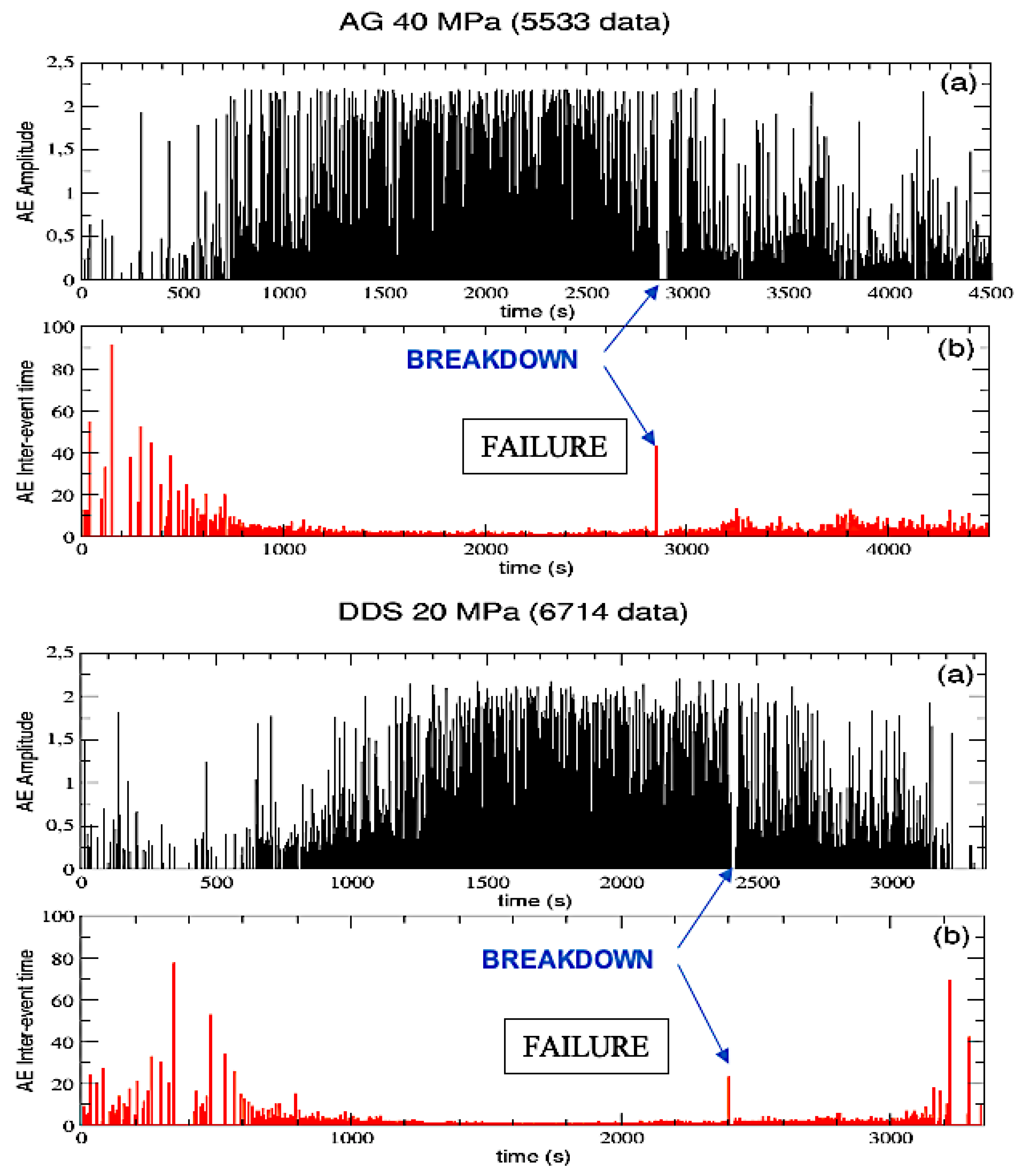
Figure 2.
Amplitude probability distributions for both AG (a) and DDS (b) and for the four increasing levels of confinement. Each data set has been divided in four time intervals, three before breakdown (0-30%, 30%-70%, 70%-100%) and the last one after failure. In the legend, for each interval and each level of confinement, the number of AE events is reported in parentheses. Only distributions extracted from more than 50 events are shown in the panels.
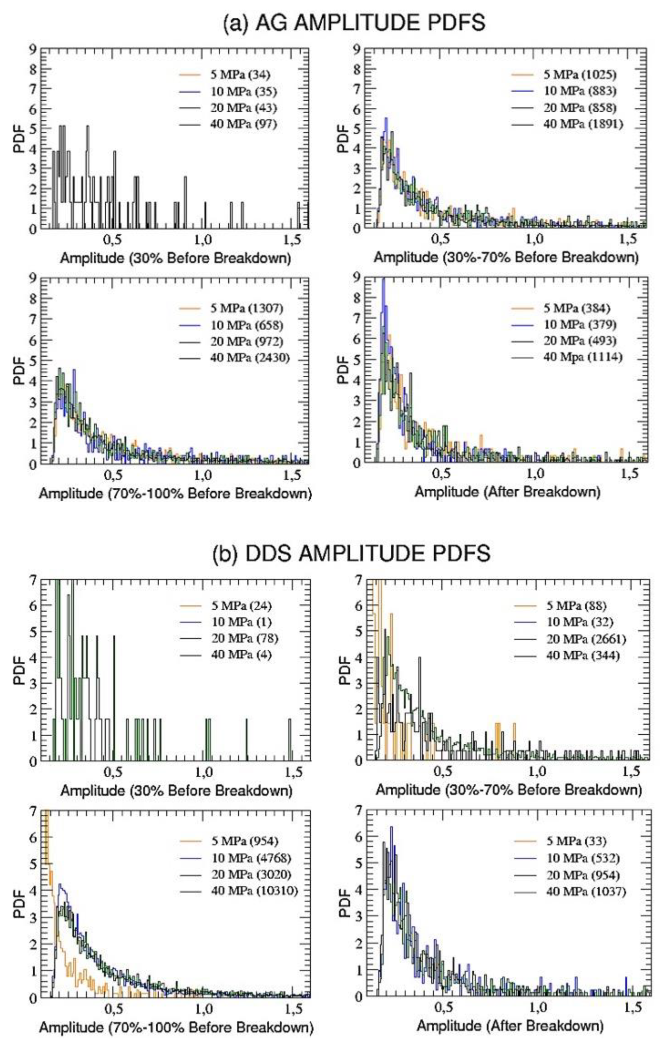
Figure 3.
Amplitude probability distributions for the entire time series of AG (a,c) and DDS (b,d) at the four levels of confinement are reported, both in Lin-Lin (a,b) and in Log-Lin (c,d) scale. The Log-Lin curves have been also fitted with a non-linear function.
Figure 3.
Amplitude probability distributions for the entire time series of AG (a,c) and DDS (b,d) at the four levels of confinement are reported, both in Lin-Lin (a,b) and in Log-Lin (c,d) scale. The Log-Lin curves have been also fitted with a non-linear function.
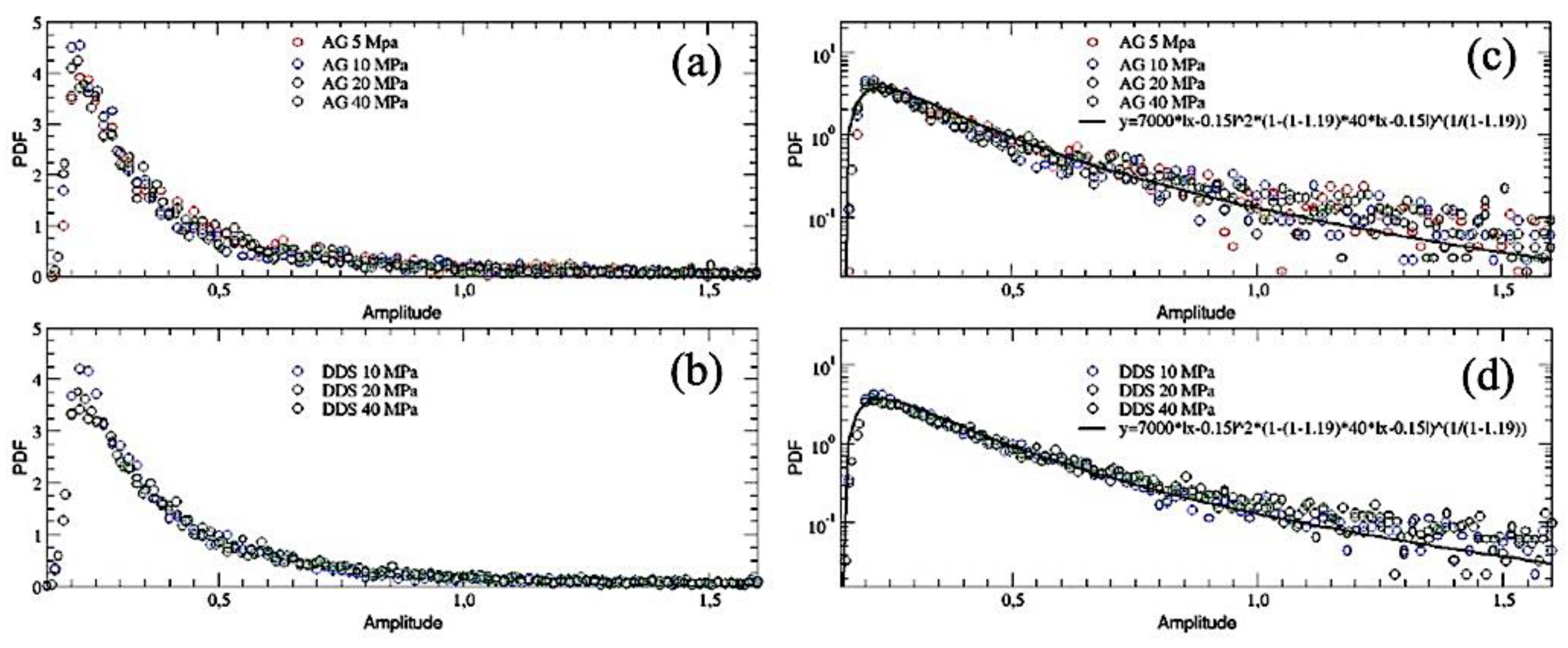
Figure 4.
AG samples: double q-exp fits for the decumulative PDFs of inter-event times.
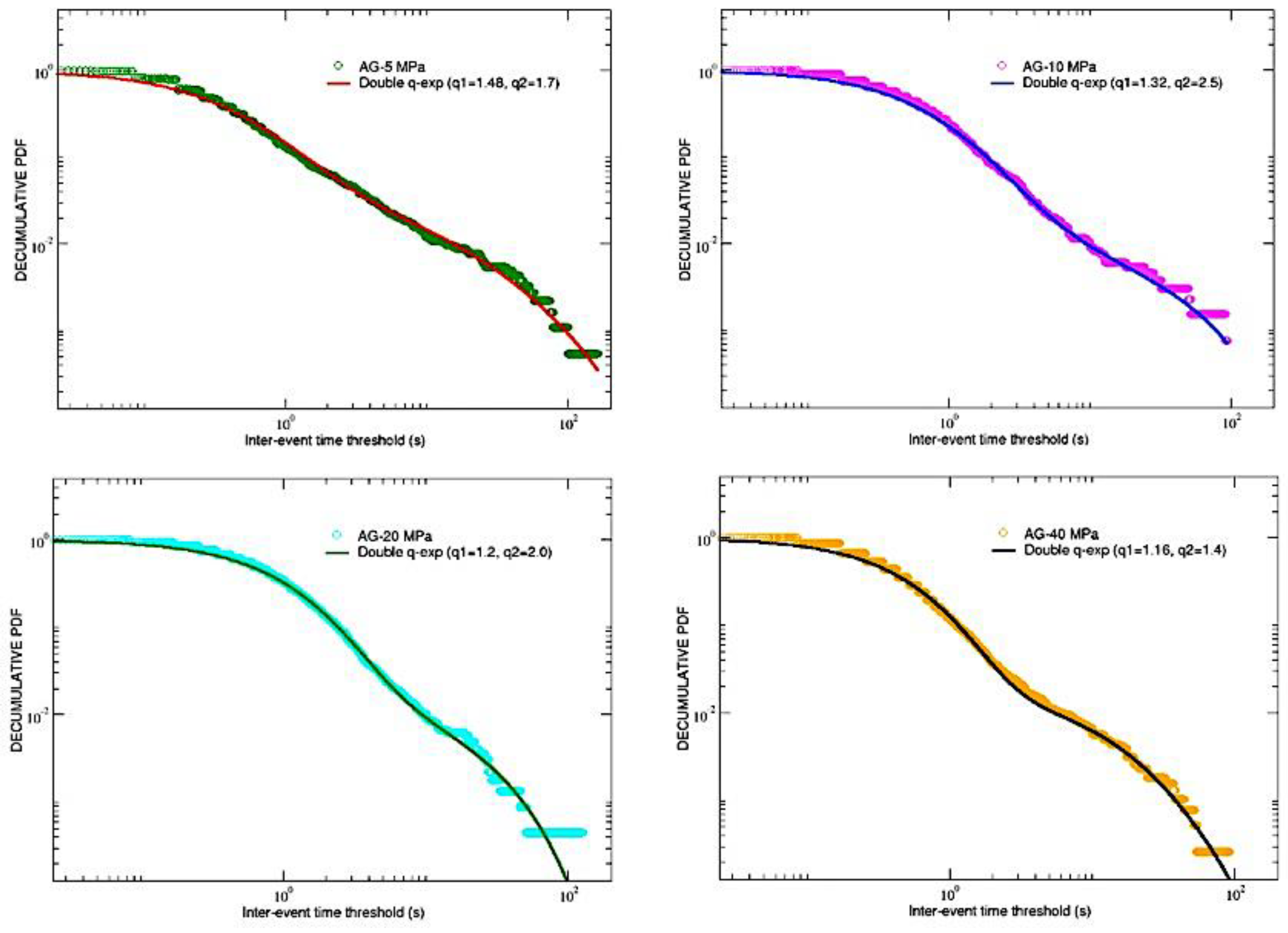
Figure 5.
DDS samples: double q-exp fits for the decumulative PDFs of inter-event times.
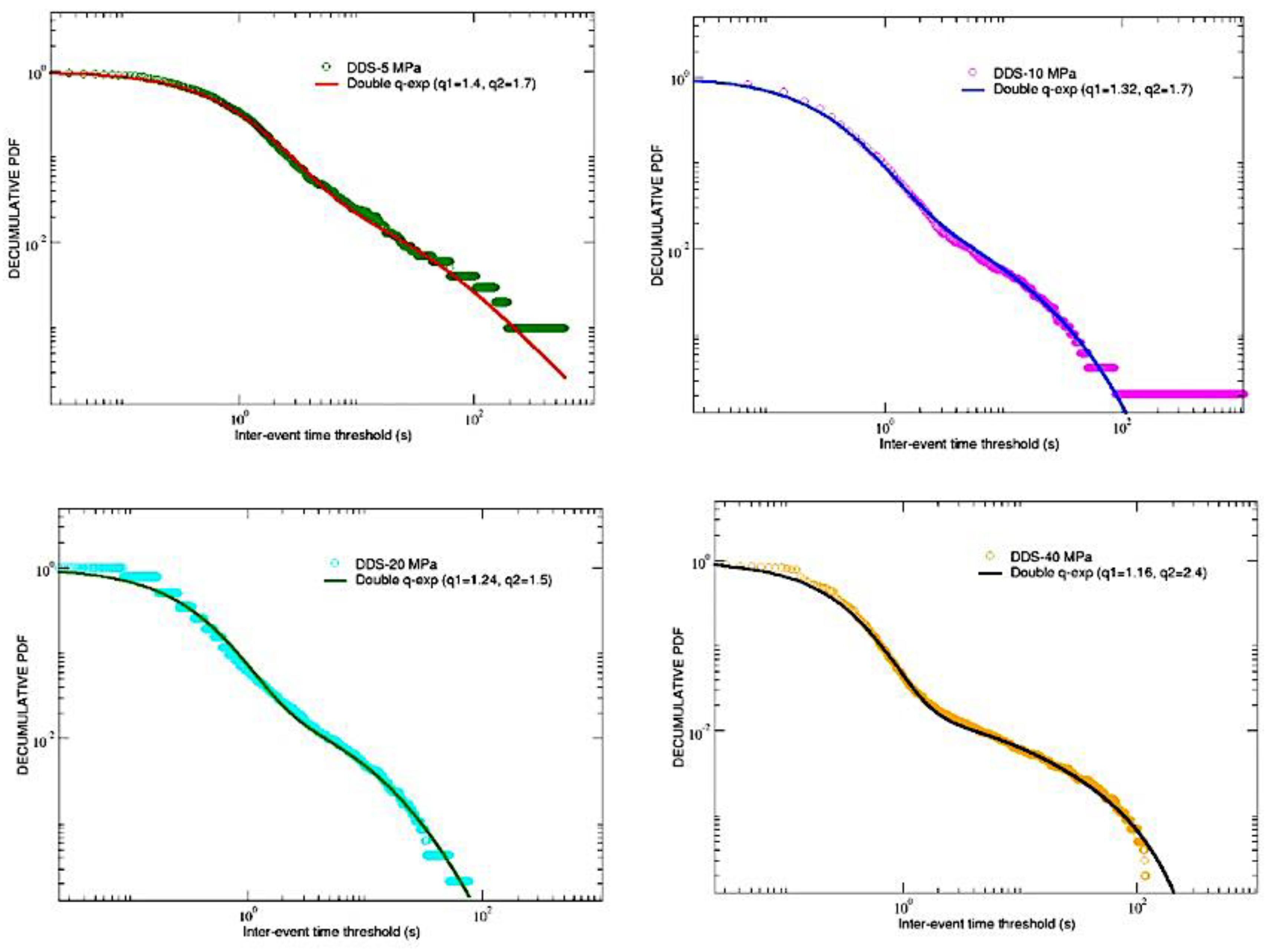
Figure 6.
Scatter plots of the time ordered positions before rupture (blue scale of decreasing intensity), projected on the three coordinate planes X-Y, X-Z and Y-Z, for AE events in the four AG samples.
Figure 6.
Scatter plots of the time ordered positions before rupture (blue scale of decreasing intensity), projected on the three coordinate planes X-Y, X-Z and Y-Z, for AE events in the four AG samples.
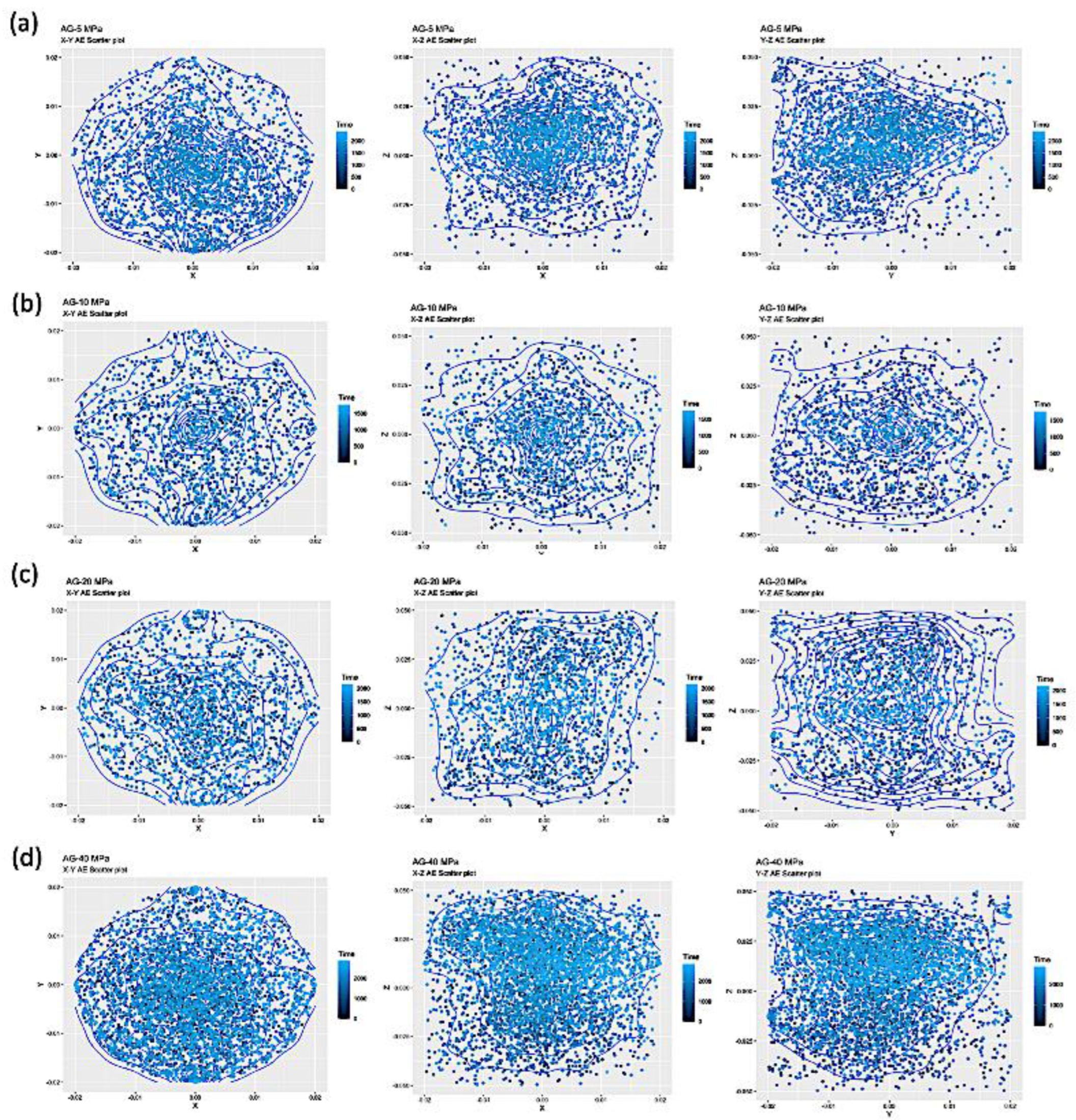
Figure 7.
Scatter plots of the time ordered positions before rupture (blue scale of decreasing intensity), projected on the three coordinate planes X-Y, X-Z and Y-Z, for AE events in the four DDS samples.
Figure 7.
Scatter plots of the time ordered positions before rupture (blue scale of decreasing intensity), projected on the three coordinate planes X-Y, X-Z and Y-Z, for AE events in the four DDS samples.
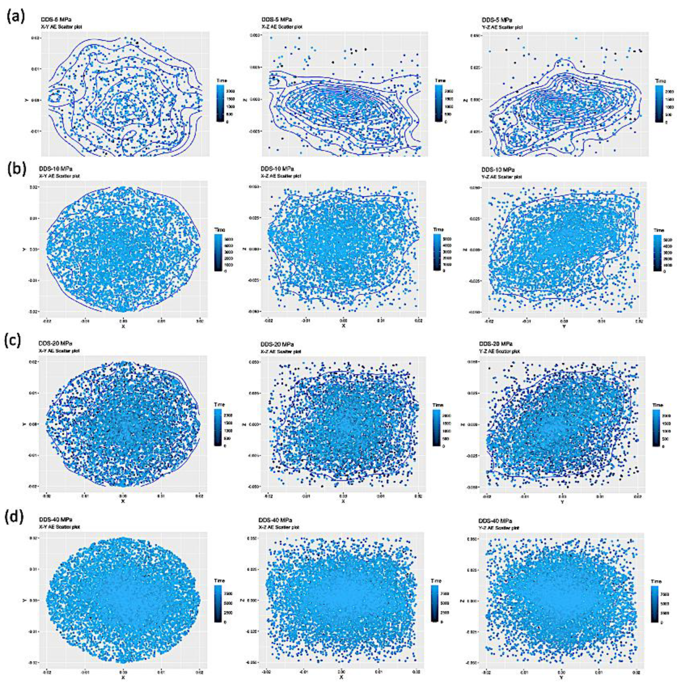
Figure 8.
PDFs of the AE inter-event distance for AG (top panel) and DDS (bottom panel) at the various levels of confinement.
Figure 8.
PDFs of the AE inter-event distance for AG (top panel) and DDS (bottom panel) at the various levels of confinement.
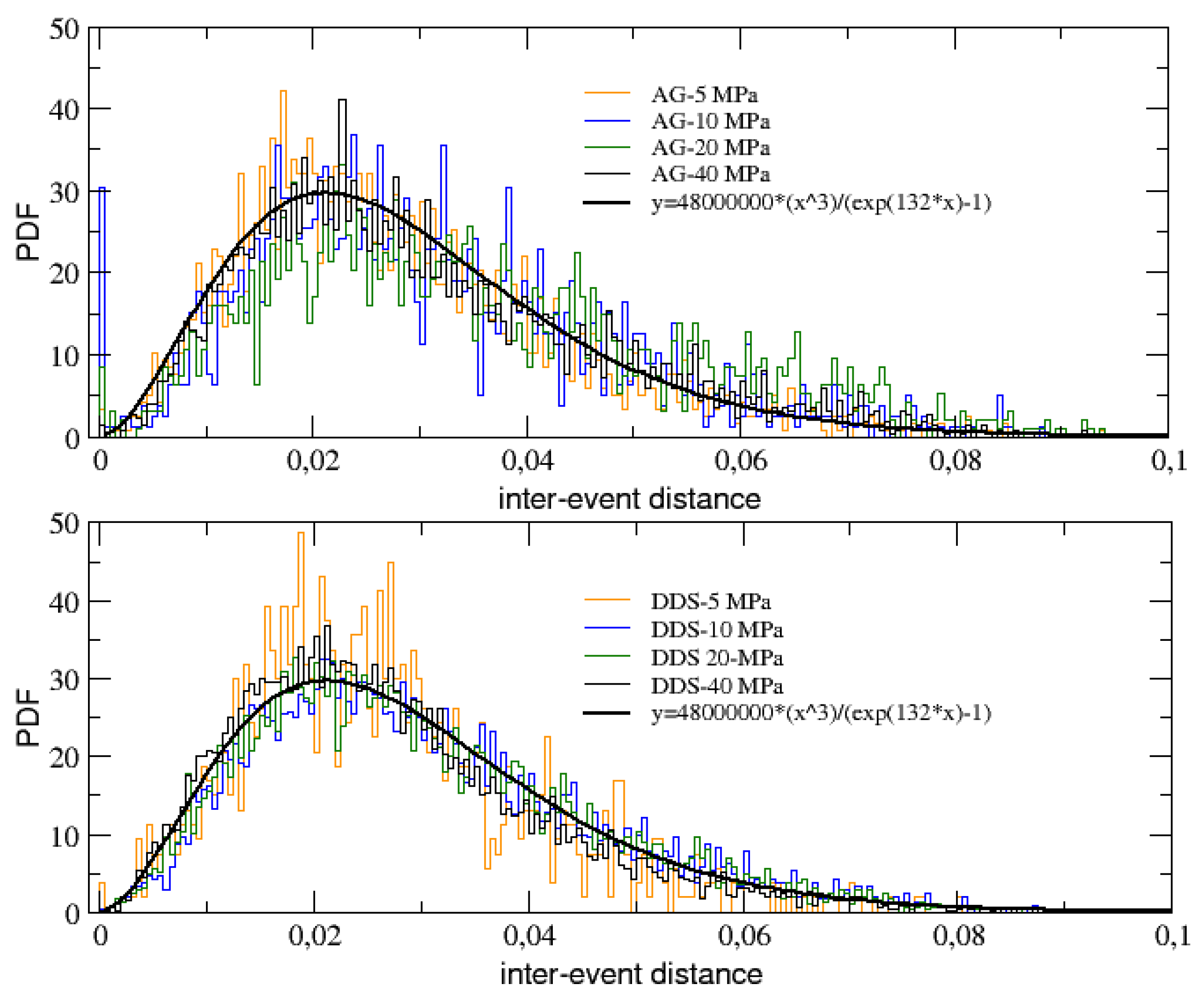
Figure 9.
AG samples: single q-exp fits for the decumulative PDFs of inter-event distances.
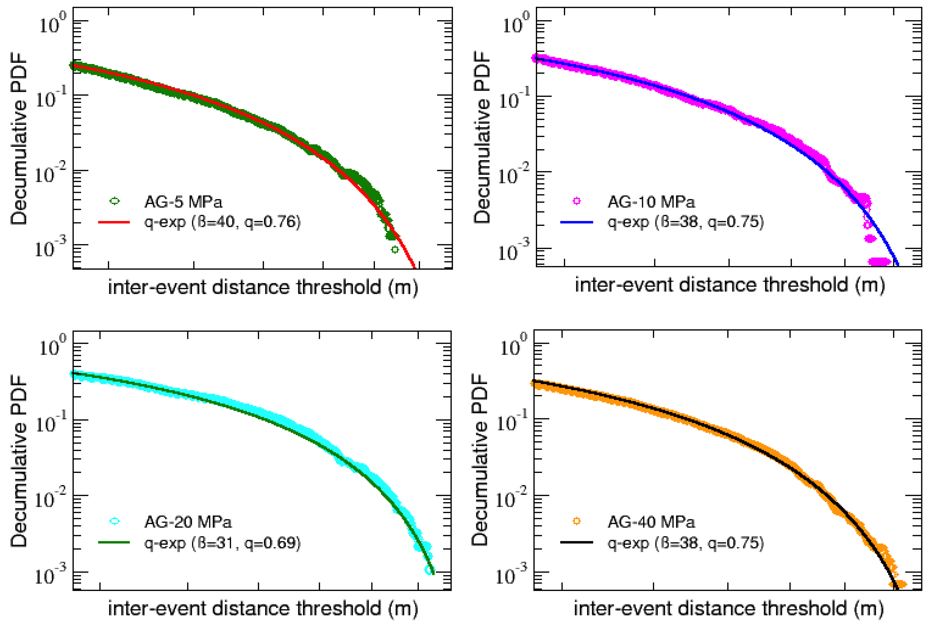
Figure 10.
DDS samples: single q-exp fits for the decumulative PDFs of inter-event distances.
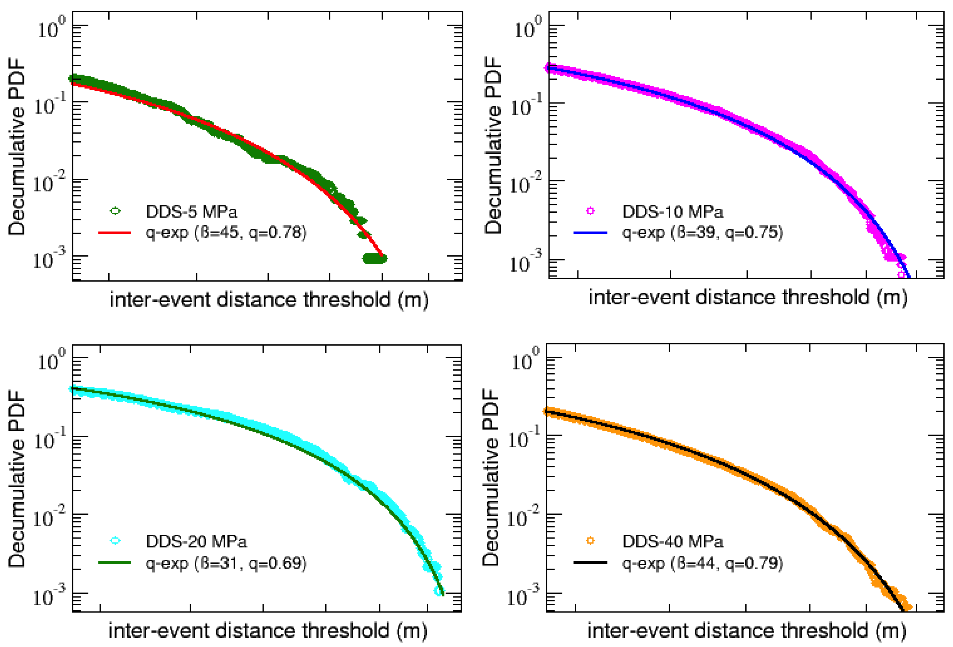
Figure 11.
The entropic index is reported as function of for the eight considered samples (colored circles) and it is compared with the line . The 10% area around the line is colored in brown.
Figure 11.
The entropic index is reported as function of for the eight considered samples (colored circles) and it is compared with the line . The 10% area around the line is colored in brown.
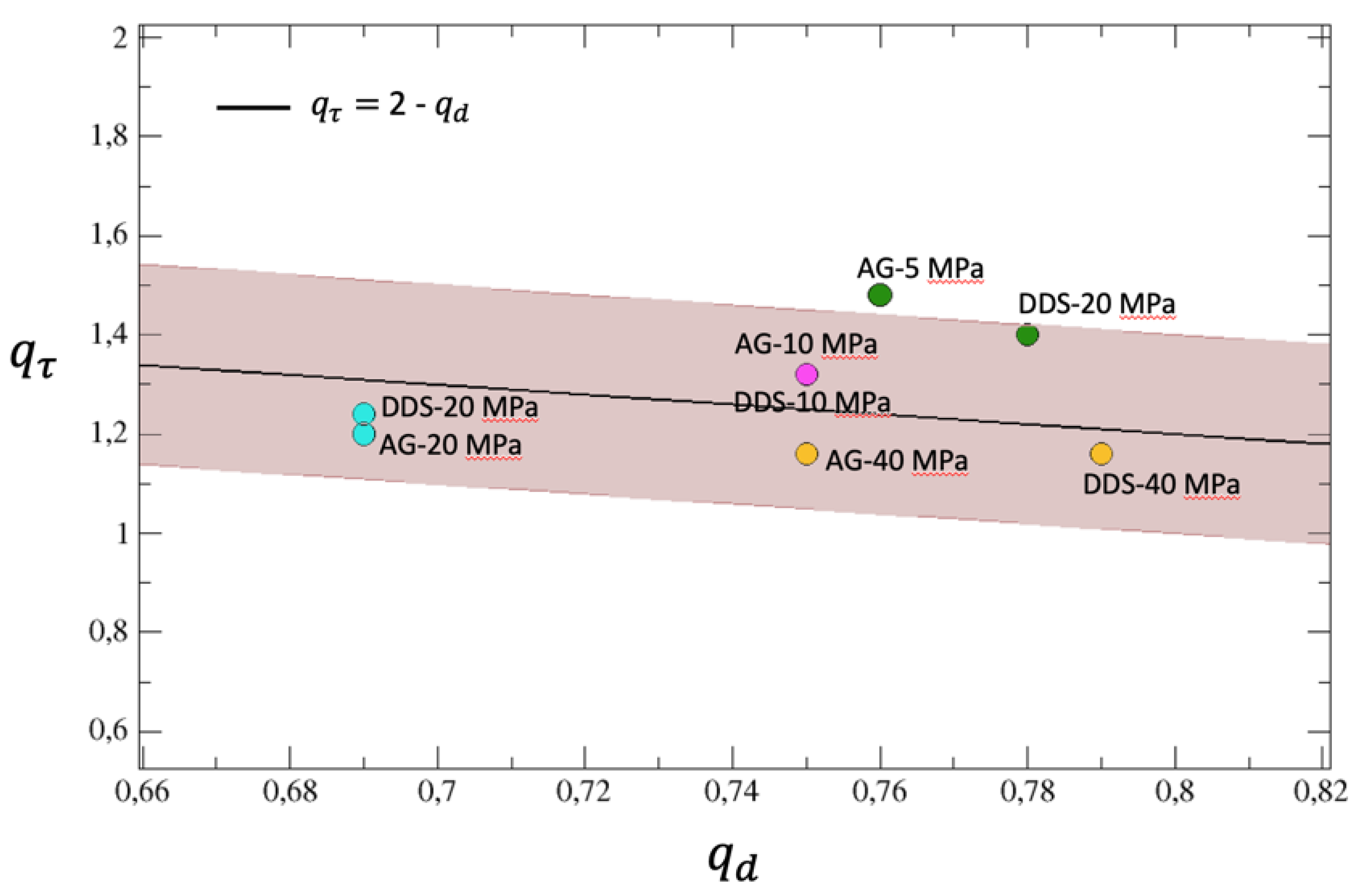

Table 1.
Details of the time series for the different samples.
| Sample | tB | tTOT | N* events before breakdown | Tot. N events |
|---|---|---|---|---|
| AG-5 MPa | 2398 s | 3395 s | 2367 | 2751 |
| AG-10 MPa | 1767 s | 2445 s | 1577 | 1956 |
| AG-20 MPa | 2160 s | 2973 s | 1874 | 2367 |
| AG-40 MPa | 2857 s | 4566 s | 4419 | 5533 |
| DDS-5 MPa | 2400 s | 2540 s | 1067 | 1100 |
| DDS-10 MPa | 5808 s | 6248 s | 4802 | 5334 |
| DDS-20 MPa | 2409 s | 3348 s | 5760 | 6714 |
| DDS-40 MPa | 9710 s | 11736 s | 10659 | 11696 |
Table 2.
Details of the fitting parameters of Equation (2) for the eight samples considered.
| Sample | ||||||
|---|---|---|---|---|---|---|
| AG-5 MPa | 0.975 | 3.5 | 1.48 | 0.01 | 1.7 | 0.09 |
| AG-10 MPa | 0.98 | 2.0 | 1.32 | 0.02 | 2.5 | 0.19 |
| AG-20 MPa | 0.98 | 1.3 | 1.2 | 0.04 | 2.0 | 0.13 |
| AG-40 MPa | 0.983 | 2.6 | 1.16 | 0.017 | 1.4 | 0.12 |
| DDS-5 MPa | 0.975 | 1.5 | 1.4 | 0.0001 | 1.7 | 0.055 |
| DDS-10 MPa | 0.98 | 4.0 | 1.32 | 0.02 | 1.7 | 0.19 |
| DDS-20 MPa | 0.98 | 4.1 | 1.24 | 0.017 | 1.5 | 0.20 |
| DDS-40 MPa | 0.983 | 4.6 | 1.16 | 0.015 | 2.4 | 0.19 |
Table 3.
The sum of the entropic indices and for the 8 considered samples oscillates around 2.
| Sample | |||
|---|---|---|---|
| AG-5 MPa | 1.48 | 0.76 | 2.24 |
| AG-10 MPa | 1.32 | 0.75 | 2.07 |
| AG-20 MPa | 1.2 | 0.69 | 1.89 |
| AG-40 MPa | 1.16 | 0.75 | 1.91 |
| DDS-5 MPa | 1.4 | 0.78 | 2.18 |
| DDS-10 MPa | 1.32 | 0.75 | 2.07 |
| DDS-20 MPa | 1.24 | 0.69 | 1.93 |
| DDS-40 MPa | 1.16 | 0.79 | 1.95 |
Disclaimer/Publisher’s Note: The statements, opinions and data contained in all publications are solely those of the individual author(s) and contributor(s) and not of MDPI and/or the editor(s). MDPI and/or the editor(s) disclaim responsibility for any injury to people or property resulting from any ideas, methods, instructions or products referred to in the content. |
© 2023 by the authors. Licensee MDPI, Basel, Switzerland. This article is an open access article distributed under the terms and conditions of the Creative Commons Attribution (CC BY) license (http://creativecommons.org/licenses/by/4.0/).
Copyright: This open access article is published under a Creative Commons CC BY 4.0 license, which permit the free download, distribution, and reuse, provided that the author and preprint are cited in any reuse.


