Submitted:
28 May 2025
Posted:
28 May 2025
Read the latest preprint version here
Abstract
Starting from a quasi-elastostatic description of a seismic activation region, it is explained how accelerating seismic release preceding a mainshock event can be described in terms of a 2D linear sigma model with phi6 self interaction. This model accounts for the discrepancy in previously reported accelerating seismic release critical exponents calculated by fracture damage mechanics and critical point models as a difference between its mean field and critical point critical scaling exponents.
Keywords:
seismic activation
; fault dynamics
; statistical physics
; signal processing
Introduction
An increase in the number of intermediate sized earthquakes () in a seismic region preceding the occurrence of an earthquake with magnitude , referred to as seismic activation, has been documented by various researchers [39]. For example, seismic activation was observed in a geographic region spanning for a period of time between 1991 and 1999 preceding the magnitude 7.6 Chi-Chi earthquake [11]. Figure 1 shows a schematic plot of the cumulative distribution of earthquakes of different magnitudes in a seismic activation region in two different time intervals of equal duration preceding occurrence of a major () earthquake at time . In this figure, is a real time parameter, and is the characteristic time of major earthquake recurrence assuming an earthquake of similar magnitude occurred in the same region at [22,30]. Importantly, the cumulative distribution of earthquakes in a time interval of fixed width increasingly deviates away from a Gutenberg-Richter linear log-magnitude plot as the end of the time interval approaches .
As a means of predicting the time at which a mainshock event preceded by seismic activation occurs, it has been hypothesized that the average seismic moment of earthquakes occuring in intervals of time preceding a mainshock event obeys an inverse power of remaining time to failure law:
and that the cumulative Benioff strain , defined as:
where is the seismic moment of the earthquake in the region starting from a time preceding the mainshock event, and is the number of earthquakes occurring in the region up to time , satisfies [28]:
The exponent selection of in Equation (2) is not necessary to derive Formula (3) with a different arithmetic relation between and , but has been selected by previous researchers based on Benioff’s finding that the elastic rebound of an earthquake is proportional to the square root of its seismic moment. When Formula (3) is fit to real seismic data, a typical value of is [29,39. Notably, validity of Equation (1) has been questioned by some researchers who claim measurements of seismic activation can be explained in terms of main event foreshock and aftershock occurrence without acceleration of seismic release [17,32].
A model of seismic activation based on fault damage mechanics (FDM) has been used to derive Equation (3) with a value [2]. In this derivation, the occurrence of seismic activation earthquakes progressively decreases the average shear modulus of fault material in the seismic region where subsequent seismic activation earthquakes occur, and the result is obtained from an equation for time evolution of the shear modulus derived from non-equilibrium thermodynamic considerations [2].
In addition to the FDM model of seismic activation, an empirical statistical physics model of seismic activation known as the Critical Point (CP) model has been put forth to derive Equation (3) with a value [22]. In this derivation, the inverse power of remaining time to failure law:
is asserted based on identifying the mean rupture length of earthquakes occuring at time with the correlation length of a statistical physical system described by Ginzburg-Landau mean field theory with a -dependent temperature parameter for which:
and relation (4) follows from the scaling relation [23]. Table 1 shows typical fault material displacements and rupture lengths for earthquakes of different moment magnitudes.
Importantly, previous work on the CP model has not explained why it is physically reasonable to describe seismic activation earthquake occurrence statistics with thermal equilibrium statistical physics formalism [26]. Therefore, the first objective of this article is to clarify how the FDM and CP models of seismic activation can be in correspondence with each other. The second objective of the article is to suggest how the presented correspondence can be tested against seismic measurements, and in the event of positive experimental verification, advance earthquake prediction technology.
Motivating the presented correspondence between FDM and CP seismic activation models is previous work demonstrating statistical physics renormalization group flow equations can, in certain cases, be identified with differential equations such as the Kolmogorov-Petrovsky-Piskunov (KPP) equation, an equation which has been used to model the time and space dependent distribution of aftershocks in a seismic region following a mainshock event [10,16]. This work may have application to earthquake prediction if it is true that 2D statistical physics critical scaling theory can be used to systematize dimensional reduction of fault dynamic models in windows of time preceding a mainshock event.
The outline of the article is as follows. Section 2 explains why it is physically reasonable to describe accelerating seismic release in terms of 2D statistical physics, and how 2D critical scaling theory is descriptive of cumulative Benioff strain in a seismic activation region. Section 3 uses critical scaling theory of the 2D linear sigma model with self interaction to explain the reported discrepancy in FDM and CP accelerating seismic release critical exponents. Section 4 concludes by commenting on how validity of statistical physics modeling of seismic activation can be tested against seismic measurements.
Materials and Methods
Seismic Activation Fault Dynamics
Figure 2 shows a 2D schematic of earthquake occurrence in a seismic activation region [19]. In this figure, the activation region is shown at 4 different times up to and including the moment after a mainshock event has occurred. At each time, black lines indicate fault ruptures associated with earthquakes that have occurred, and red lines indicate faults where shear strain is accumulating prior to earthquake occurrence. Qualitatively, the picture suggests the occurrence of successively larger earthquakes, associated with successively longer rupture lengths, leads to increased strain along the mainshock fault as seismic activation proceeds. From an FDM point of view, this increased strain occurs with a reduction in the average shear modulus of material in the vicinity of the fault, until fault rupture occurs at time .
Quantitatively, this picture of seismic activation leading to rupture along a mainshock fault is supported by modeling of earthquake fault dynamics in 1+1 spacetime dimensions, whereby the differential equation:
has been used to model both creep along an earthquake fault and rupture propagation, depending on whether or not frictional forces dominate the fault dynamics and shear stress evolution along the fault is more appropriately described with a reaction diffusion equation or a solitary wave equation [2]. In this equation, is real time, z coordinates a direction of creep or slip along an earthquake fault, is the local displacement of elastic material across the earthquake fault, is the local inertial force acting on the fault material, is the local elastic restoring force acting on the fault material, and and are local frictional forces acting on the fault material attributed to contact of the material with tectonic plates on either side of the fault. For , an (anti-kink) soliton solution to equation can be interpreted as propagation of earthquake fault rupture.
To generalize this description of fault creep and rupture in 1 spatial dimension to 3 spatial dimensions, assume that for , material constituting the seismic activation region undergoes a quasi-elastostatic finite strain deformation, whereby at any moment in time it exists in an elastostatic equilibrium configuration in which strain energy is minimized . With this assumption, if the seismic activation region is ascribed a finite element mesh, a nodal displacement of the region’s equilibrium configuration at tme increases the strain energy of the region by:
for equal to the positive definite stiffness matrix of the region at time . For , has N eigenvalues , where N is the number of finite element mesh nodes. At , has at least one zero eigenvalue identifying a marginally stable seismic displacement that describes the mainshock faulti rupture [9]. If we now further suppose that in the limit , a subset of the eigenvalues of , including , have eigenvectors with 0 nodal displacement outside of a seismic activation subregion containing the mainshock fault, it follows that the subregion has a stiffness matrix that may be isospectral for with real time evoution determined by a solitonic Lax pair [18].
Statistical Physics Critical Scaling Theory
From a classical deterministic view of the seismic activation region, its stiffness matrix eigenvalues undergo a deterministic motion of N points on the real line. However, if we instead view the evolution of the seismic activation region elastic model as a stochastic process in which is selected from a -dependent ensemble of random matrices, a corresponding description of the stiffness matrix eigenvalue evolution must be probabilistic. Therefore, the objective herin is to investigate whether or not real time evolution of the stiffness matrix eigenvalue distribution can be described in terms of statistical physics models, whereby convergence of the stiffness matrix eigenvalue distribution to an isopsectral distribution at corresponds to invariance of statistical physics model coefficients at a renormalization group fixed point.
Qualitatively, the eigenvalues of the stiffness matrix depend on the material composition of the activation region, the level of fracture induced damage of material, and the level of stress/strain applied to material, with fracture induced damage dominating relative elastic parameter changes at seismic wavelengths short in comparison to the mainshock rupture length throughout activation, and applied stress/strain dominating relative elastic parameter changes at long seismic wavelengths just preceding the mainshock. Supposing the fracture induced damage steadily increases throughout seismic activation, as may be quantified by real time variation of seismic wave scattering coefficients, it is possible that some subset of the eigenvalues of exhibit level repulsion, whereby their distribution is determined by a Wigner-Dyson-Gaudin-Mehta invariant matrix ensemble (IME) with parameter steadily decreasing as . Moreover, the IME distribution for can be interpreted as the ground state wave function of a system of non-interacting fermions in 1 spatial dimension in an external harmonic potential. Based on this fact, it is hereby conjectured that the statistical distribution of some subset of the eigenvalues of is specified by the ground state wave function of a system of non-interacting fermions in 1 spatial dimension in an external potential , where is a bosonic field in 1+1 spacetime dimensions that mediates interaction between the fermions. This conjecture allows for previously reported claims that progression of seismic activation can be described in terms of statistical physics critical scaling theory, assuming the spatial domain of the statistical physics model is 2D, and the statistical physics model is related to the 1+1D bosonic field theory by Wick rotation [21].
Assuming nodal material displacement is measured relative to the seismic activation region’s unstable configuration at , and sampled at a frequency lower than the corner frequency of the mainshock event (1-2Hz for moment magnitude 7), each component of material strain can be computed and averaged across the activation region to determine a strain function of frequency valid above a low frequency cutoff. For the purpose of modeling seismic activation, it is now further conjectured that the spatially averaged component of shear strain across the mainshock fault plane in the direction of main event slip is , whereby critical scaling of the cumulative Benioff strain in time corresponds to critical scaling of the field in time. From this point of view, a 1+1D field theoretic description of can be interpreted as a description of how strain across an activation subregion of diameter depends on the level of fracture damage at time . This description is `effective’ in that it is accurate during intermediate stages of seismic activation, but incorrect in a window of time immediately preceding the mainshock event, during which time a `bare’ field theoretic description of strain accumulation in the seismic activation region is required to accurately compute the cumulate Benioff strain critical exponent [15].
Results
The 2D linear sigma model with self interaction is described by the Landau free energy functional:
where the constant is zero at temperature when , and negative for . If it is further assumed that at the time of the mainshock event, the mean field Landau free energy density associated with this functional is:
where is the mean field value of . This theory implies the mean field scaling relation:
is valid for intermediate stages of seismic activation, recovering the CP cumulative Benioff strain scaling relation. Appreciating that the CP model is a mean field theoretic description of accelerating seismic release, it now follows that the difference between CP and FDM accelerating seismic release critical scaling exponents is accounted for by anomalous critical scaling of a 2D statistical physics model underlying the effective 2D linear sigma model that is valid in the critical region corresponding to times .
Discussion
Previous research has identified predicting the time of occurrence of mainshock events as an application of statistical physics models of seismic activation, but this application has not yet been realized [39. In more recent times, the artificial intelligence algorithm QuakeGPT has been developed for the purpose of forecasting earthquake occurrence, using seismic event record training data created with a stochastic simulator [2,13,24]. Therefore, a practical application of statistical physics models of seismic activation may be to be improve stochastic simulation of seismic event records for use in earthquake forecasting technology, acknowledging that rigorous tests of model validity against real seismic data must be passed before achieving this objective can be considered a realistic possibility.
From a geophysical testing point of view, if it is true that the real time evolution of a seismic activation region elastic model preceding a mainshock can be quantified using a 2D statistical physics model renormalization group flow, expressible as a nonlinear dynamical system of finite phase space dimension, a geophysical signal processing technique known as singular spectrum analysis should apply to determine this phase space dimension [2]. More specifically, it is suggested that measurements of relative changes in seismic wave velocity be performed between pairs of seismic stations in a seismic region at regular time intervals during a seismic activation series, and used as input to a time domain multichannel singular spectrum analysis algorithm [20]. The number of channels of this algorithm should equate to the number of station pairs, and the number of singular values output by the algorithm in different time windows preceding a mainshock event should count the number of unstable stress/strain modes contributing to rupture nucleation if the statistical physics model of seismic activation is correct in principle. With reference to previous geophysical application of singular spectrum analysis, performed in the frequency domain, the signal processing algorithm suggested here is different in that it should be carried out in the time domain rather than the frequency domain [25].
In conclusion, work towards improving current earthquake early warning systems can proceed in two directions. Firstly, work can be done to determine whether or not observed changes of the Earth’s elastic velocity model preceding mainshock events can be processed to extract an integer identifiable as the phase space dimension of a nonlinear dynamical system. Secondly, work can be done to elaborate upon the statistical physics mathematical model of seismic activation presented in this article to determine other tests of its scientific validity and potential for practical application.
Author Contributions
Not applicable.
Funding
This research received no external funding.
Institutional Review Board Statement
Not applicable.
Informed Consent Statement
Not applicable.
Acknowledgments
Thanks to my family for their support throughout completion of this research. Thanks to Dr. Girish Nivarti, Dr. Evans Boney, and Professor Richard Froese for their willingness to entertain communication regarding the content of the article.
Conflicts of Interest
The authors declare no conflicts of interest.
Abbreviations
The following abbreviations are used in this manuscript:
| MDPI | Multidisciplinary Digital Publishing Institute |
| DOAJ | Directory of open access journals |
| TLA | Three letter acronym |
| LD | Linear dichroism |
References
- Bena, I.; Droz, M.; Lipowski, A. Statistical mechanics of equilibrium and nonequilibrium phase transitions: the Yang–Lee formalism. International Journal of Modern Physics B 2005, 19, 4269–4329. [Google Scholar] [CrossRef]
- Ben-Zion, Y. Collective behavior of earthquakes and faults: Continuum-discrete transitions, progressive evolutionary changes, and different dynamic regimes. Reviews of Geophysics 2008, 46. [Google Scholar] [CrossRef]
- Ben-Zion, Y.; Lyakhovsky, V. Accelerated seismic release and related aspects of seismicity patterns on earthquake faults. Earthquake processes: Physical modelling, numerical simulation and data analysis Part II 2002, 2385–2412. [Google Scholar]
- Bindel, D.S. Structured and parameter-dependent eigensolvers for simulation-based design of resonant MEMS Doctoral dissertation. University of California, Berkeley. 2006.
- Bose, M.; Andrews, J.; Hartog, R.; Felizardo, C. Performance and next-generation development of the finite-fault rupture detector (FinDer) within the United StatesWest Coast ShakeAlert warning system. Bulletin of the Seismological Society of America 2023, 113, 648–663. [Google Scholar] [CrossRef]
- Bowman, D.; Ouillon, G.; Sammis, C.; Sornette, A.; Sornette, D. An observational test of the critical earthquake concept. Journal of Geophysical Research: Solid Earth 1998, 103, 24359–24372. [Google Scholar] [CrossRef]
- Broomhead, D.S. ; KingGP Extracting qualitative dynamics from experimental data. Physica D: Nonlinear Phenomena 1986, 20, 217–236. [Google Scholar] [CrossRef]
- Bykov, V.G. Solitary waves on a crustal fault. Volcanology and Seismology 2001, 22, 651–661. [Google Scholar]
- Carlson, J.M.; Langer, J.S. Properties of earthquakes generated by fault dynamics. Physical Review Letters 1989, 62, 2632. [Google Scholar] [CrossRef] [PubMed]
- Carpentier, D.; Le, D.o.u.s.s.a.l.P. Disordered XY models and Coulomb gases: renormalization via traveling waves. Physical review letters 1998, 81, 2558. [Google Scholar] [CrossRef]
- Chen, C.C. Accelerating seismicity of moderate-size earthquakes before the 1999 Chi-Chi, Taiwan, earthquake: Testing time-prediction of the self-organizing spinodal model of earthquakes. Geophysical Journal International 2003, 155, F1–5. [Google Scholar] [CrossRef]
- Coleman, S. Fate of the false vacuum: Semiclassical theory. Physical Review D 1977, 15, 2929. [Google Scholar] [CrossRef]
- Cua, G.; Heaton, T. The Virtual Seismologist (VS) method: A Bayesian approach to earthquake early warning. In Earthquake Early Warning Systems, Eds. Gasparini P, Manfredi G, and Zschau J; Springer: Berlin and Heidelberg, Germany, 2007; pp. 97–132. [Google Scholar]
- Erdos, L. Random matrices, log-gases and Holder regularity. arXiv 2014, arXiv:1407.5752. [Google Scholar]
- Goldenfeld, N. Continuous Symmetry. In Lectures on phase transitions and the renormalization group; CRC Press, 2018; pp. 335–350.
- Guglielmi, A.V.; Klain, B.I.; Zavyalov, A.D.; Zotov, O.D. A Phenomenological theory of aftershocks following a large earthquake. Journal of Volcanology and Seismology 2021, 15, 373–378. [Google Scholar] [CrossRef]
- Hardebeck, J.L.; Felzer, K.R.; Michael, A.J. Improved tests reveal that the accelerating moment release hypothesis is statistically insignificant. J. Geophys. Res. 2008, 113. [Google Scholar] [CrossRef]
- Kasman, A. Glimpses of soliton theory: the algebra and geometry of nonlinear PDEs; American Mathematical Society, 2023.
- Lei, Q.; Sornette, D. Anderson localization and reentrant delocalization of tensorial elastic waves in twodimensional fractured media. Europhys. Letters 2022, 136, 1–7. [Google Scholar]
- Merrill, R.J.; Bostock, M.G.; Peacock, S.M.; Chapman, D.S. Optimal multichannel stretch factors for estimating changes in seismic velocity: Application to the 2012 Mw 7.8 Haida Gwaii earthquake. Bulletin of the Seismological Society of America 2023, 113, 1077–1090. [Google Scholar] [CrossRef]
- Peskin, M.E. An introduction to quantum field theory. CRC press. 2018.
- Rundle, J.B.; Klein, W.; Turcotte, D.L.; Malamud, B.D. Precursory seismic activation and critical-point phenomena. Microscopic and Macroscopic Simulation: Towards Predictive Modelling of the Earthquake Process 2001, 2165–2182. [Google Scholar]
- Rundle, J.B.; Turcotte, D.L.; Shcherbakov, R.; Klein, W.; Sammis, C. Statistical physics approach to understanding the multiscale dynamics of earthquake fault systems. Reviews of Geophysics 2003, 41. [Google Scholar] [CrossRef]
- Rundle, J.B.; Fox, G.; Donnellan, A.; Ludwig, I.G. Nowcasting earthquakes with QuakeGPT: Methods and first results. In Scientific Investigation of Continental Earthquakes and Relevant Studies; Springer Nature: Singapore, 2025. [Google Scholar]
- Sacchi, M. FX singular spectrum analysis. In Cspg Cseg Cwls Convention, 392–395.
- Saleur, H.; Sammis, C.; Sornette, D. Renormalization group theory of earthquakes. Nonlinear Processes in Geophysics 1996, 3, 102–109. [Google Scholar] [CrossRef]
- Schoenberg, M. Elastic wave behavior across linear slip interfaces. The Journal of the Acoustical Society of America 1980, 68, 1516–1521. [Google Scholar] [CrossRef]
- Tzanis, A.; Vallianatos, F.; Makropoulos, K. Seismic and electrical precursors to the 17-1-1983, M7 Kefallinia earthquake, Greece: Signatures of a SOC system. Physics and Chemistry of the Earth, Part A: Solid Earth and Geodesy 2000, 25, 281–287. [Google Scholar] [CrossRef]
- Vallianatos, F.; Chatzopoulos, G. A complexity view into the physics of the accelerating seismic release hypothesis: Theoretical principles. Entropy 2018, 20, 754. [Google Scholar] [CrossRef] [PubMed]
- Vallianatos, F.; Sammonds, P. Evidence of non-extensive statistical physics of the lithospheric instability approaching the 2004 Sumatran–Andaman and 2011 Honshu mega-earthquakes. Tectonophysics 2004, 590, 52–58. [Google Scholar] [CrossRef]
- Wu, R.S.; Aki, K. Scattering characteristics of elastic waves by an elastic heterogeneity. Geophysics 1985, 50, 582–595. [Google Scholar] [CrossRef]
- Zhou, S.; Johnston, S.; Robinson, R.; Vere-Jones, D. Tests of the precursory accelerating moment release model using a synthetic seismicity model for Wellington, New Zealand. J. Geophys. Res. 2006, 111. [Google Scholar]
Figure 1.
Plot of the cumulative distribution of earthquakes of different moment magnitudes in a seismic zone in two different time intervals of equal width preceding occurrence of a major earthquake at [22,30].
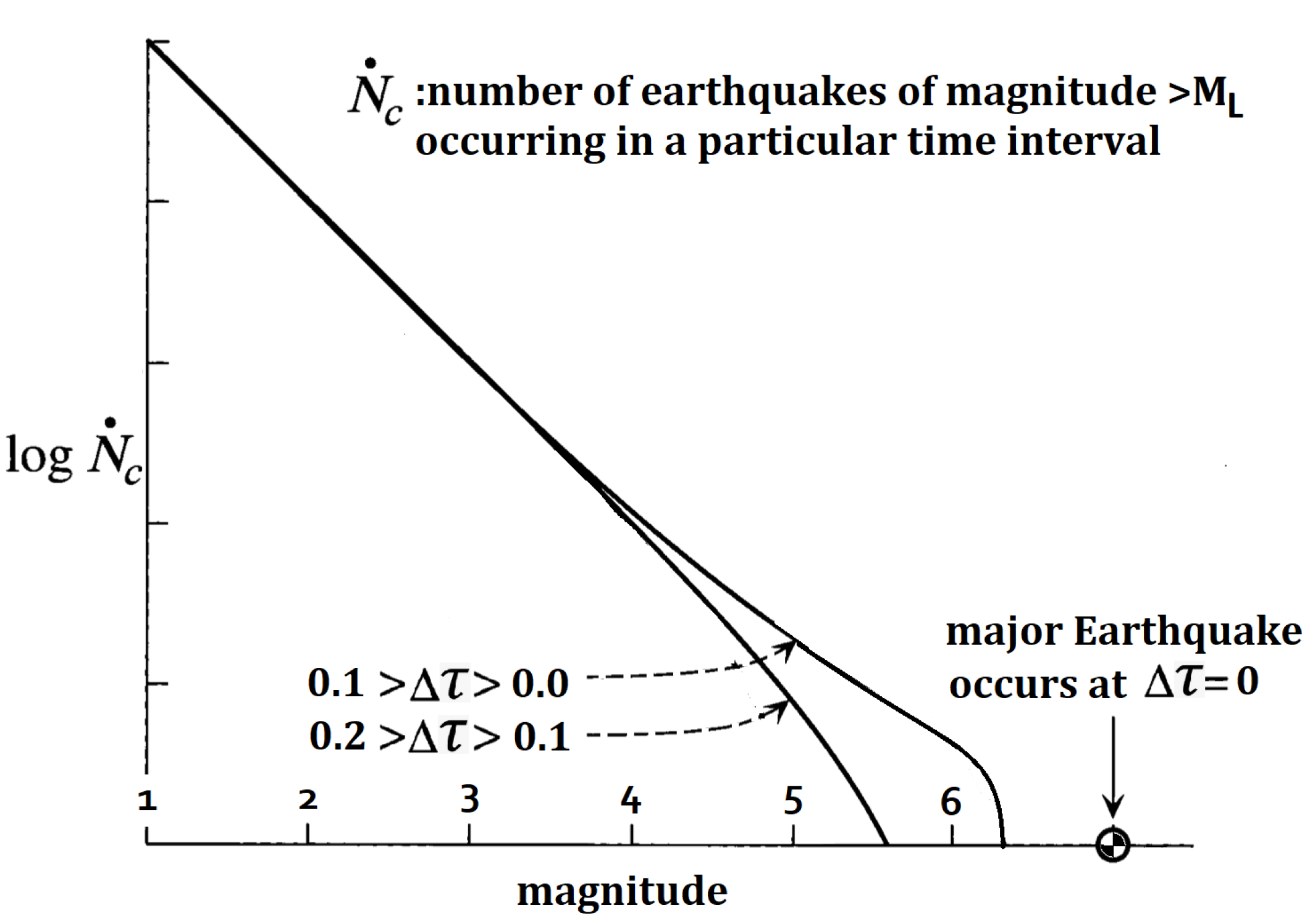
Figure 2.
Schematic illustration of seismic activation in a 2D geometry at four different times in which each black line represents an earthquake fault rupture that has already occured, and the red lines represent earthquake faults along which shear stress is increasing prior to rupture [19].
Figure 2.
Schematic illustration of seismic activation in a 2D geometry at four different times in which each black line represents an earthquake fault rupture that has already occured, and the red lines represent earthquake faults along which shear stress is increasing prior to rupture [19].
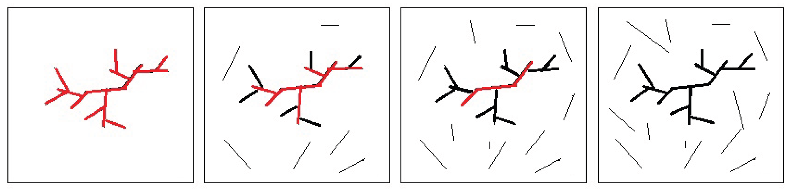

Table 1.
Approximate relation between earthquake magnitude, fault material displacement, and fault rupture length.
Table 1.
Approximate relation between earthquake magnitude, fault material displacement, and fault rupture length.
| Moment Magnitude | Average Fault Material Displacement (m) | Fault Rupture Length (km) |
|---|---|---|
| 4 | 0.05 | 1 |
| 5 | 0.15 | 3 |
| 6 | 0.5 | 10 |
| 7 | 1.5 | 30 |
| 8 | 5 | 100 |
Disclaimer/Publisher’s Note: The statements, opinions and data contained in all publications are solely those of the individual author(s) and contributor(s) and not of MDPI and/or the editor(s). MDPI and/or the editor(s) disclaim responsibility for any injury to people or property resulting from any ideas, methods, instructions or products referred to in the content. |
© 2025 by the authors. Licensee MDPI, Basel, Switzerland. This article is an open access article distributed under the terms and conditions of the Creative Commons Attribution (CC BY) license (http://creativecommons.org/licenses/by/4.0/).
Copyright: This open access article is published under a Creative Commons CC BY 4.0 license, which permit the free download, distribution, and reuse, provided that the author and preprint are cited in any reuse.


