
Submitted:
06 February 2025
Posted:
07 February 2025
You are already at the latest version
Abstract
Carbon capture, utilisation and storage technologies are increasingly recognized as crucial components in the global strategy to mitigate climate change. As the deployment of carbon capture, utilisation and storage systems expands, there is a growing need for rigorous monitoring and verification methods to ensure that these technologies achieve their intended reduction in greenhouse gas emissions. This paper explores the current state of monitoring techniques for carbon capture, utilisation and storage facilities, highlighting the challenges and opportunities associated with accurately quantifying net greenhouse gas emissions. We analyse both traditional bookkeeping methods and direct measurement techniques. Our analysis reveals the limitations of current monitoring frameworks and underscores the importance of integrating advanced measurement technologies, such as in-situ sensors, drones and satellite observations, to enhance the accuracy and reliability of greenhouse gas reporting. By proposing a comprehensive monitoring strategy that combines these methods, we aim to provide a roadmap for more effective oversight of carbon capture, utilisation and storage facilities, thereby contributing to the broader goal of reducing global carbon emissions.
Keywords:
carbon capture
; utilisation and storage (CCUS)
; greenhouse gas monitoring
; remote sensing technologies
; climate change mitigation
1. Introduction
The global imperative to combat climate change has catalyzed the widespread adoption of carbon capture, utilisation and storage (CCUS) technologies across various industries and sectors worldwide. These technologies have emerged as indispensable tools in the pursuit of achieving the ambitious targets outlined in the Paris Agreement [1]. As nations intensify their efforts to curb greenhouse gas (GHG) emissions and transition towards sustainable energy systems, CCUS has garnered significant attention and investment, particularly within industrial and energy-intensive sectors [2].
The multifaceted nature of CCUS technologies allows for diverse applications, ranging from direct air capture [3] to sequestration of emissions at large-scale industrial facilities for utilising the CO2 for enhanced oil recovery [EOR, [4] and synthesis of valuable compounds [5]. With the potential to significantly reduce emissions while contributing to economic growth, CCUS has become increasingly integrated into national and international climate mitigation strategies.
While CCUS holds promise to mitigate GHG emissions and facilitate the transition to a low-carbon economy, its effectiveness hinges on rigorous monitoring and verification to ensure that net emissions reductions are achieved. Given the substantial energy requirements of CCUS processes, which often rely on fossil fuels, there is a pressing need to monitor and verify the actual reduction in GHG emissions achieved by these facilities. However, accurately quantifying the net emissions from CCUS operations presents several complex challenges that must be addressed.
Traditional methods of monitoring GHG emissions typically employ bookkeeping approaches, which estimate emissions based on process data, emission factors and other parameters. While these methods serve as valuable tools for providing a baseline estimate of emissions, they may underestimate actual emissions due to factors such as leakage, process inefficiencies and unaccounted sources. For example, the Global Methane Project has highlighted the inherent limitations of bookkeeping methods in accurately quantifying emissions [6]. Similarly, a recent validation of Denmark’s inventory reports using satellite data revealed that actual emissions were 56–75% higher than reported estimates [7].
To address the inherent uncertainties associated with bookkeeping methods and provide a more accurate assessment of net GHG emissions from CCUS facilities, direct measurement techniques are receiving a growing emphasis. Direct measurement methods, such as in-situ monitoring [8] and remote sensing [9], offer the advantage of providing real-time data on emissions, enabling prompt identification of leaks and verification of emission reductions. These methods complement bookkeeping approaches by providing independent verification of emission estimates and enhancing overall transparency and accountability in GHG reporting.
In this study, our overarching objective is to examine the growing imperative for monitoring overall GHG emissions from CCUS facilities and explore the pivotal role exerted by direct measurement techniques in achieving this objective. We will meticulously assess the strengths and limitations of both bookkeeping and direct measurement methods and elucidate their implications for accurately quantifying and verifying GHG emissions reductions from CCUS operations. Through a comprehensive analysis, we endeavor to provide invaluable insights into best practices for monitoring and reporting GHG emissions from CCUS facilities, thereby bolstering global efforts towards more effective climate mitigation strategies.
2. Current Activities
In fall 2023 there were all over the world around 40 CCUS facilities in operation with a total capture capacity of more than 45 MtCO2 according to the International Energy Agency [10]. In addition, there were over 700 projects in various stages of development. Most of these facilities are constructed in connection with natural gas processing plants and EOR plants, where it is relatively easy to capture the CO2. However, a growing number of bioenergy facilities with carbon capture and storage (BECCS) and direct air capture (DAC) facilities are being planned. Most of these facilities are based on dedicated geological storage. Both the operating and the planned facilities are found both off and on shore.
When evaluating the net result of a given facility, it is important to include in the calculation both the sink and emissions. In this way, it appears that facilities based on EOR does not necessarily have a positive net result, since the CO2 that they remove from the atmosphere is injected into the ground for boosting the extraction of hydrocarbons, whose combustion will however again emit CO2. Similar considerations need to be drawn for other types of facilities like BECCS and DAC. In the first case, the production of bioenergy might lead to large methane emissions while, for DAC, the production of the energy needed for the sequestration could be associated with large emission.
In order to evaluate the net result of a given facility it is thus important to have a Measurement, Monitoring and Verification (MMV) program that is capable of taking into account of both the sink and the emissions associated with a given facilities.
There are two overall reasons, why a CCUS facility needs an MMV program:
- Documentation for legislation
- Documentation carbon emission trading
Below we will go through the requirements needed for the two kinds of documentation.
2.1. Requirements for Legislation
The Global CCS Institute maintains a CCS Legal and Regulatory Indicator (the CCS-LRI), which is described in Havercroft [11]. The indicator described the state of CCS-specific laws or existing laws that are applicable across most parts of the CCS project cycle. Countries like Australia, Canada, Denmark, United Kingdom and USA score high on this indicator. In general, most European countries score high on the indicator, which is likely related to the EU CCS directive that has been in place since 2009 and had to be transposed into national law by June 2011. In the following we go through the main points in the EU CCS directive.
Figure 1.
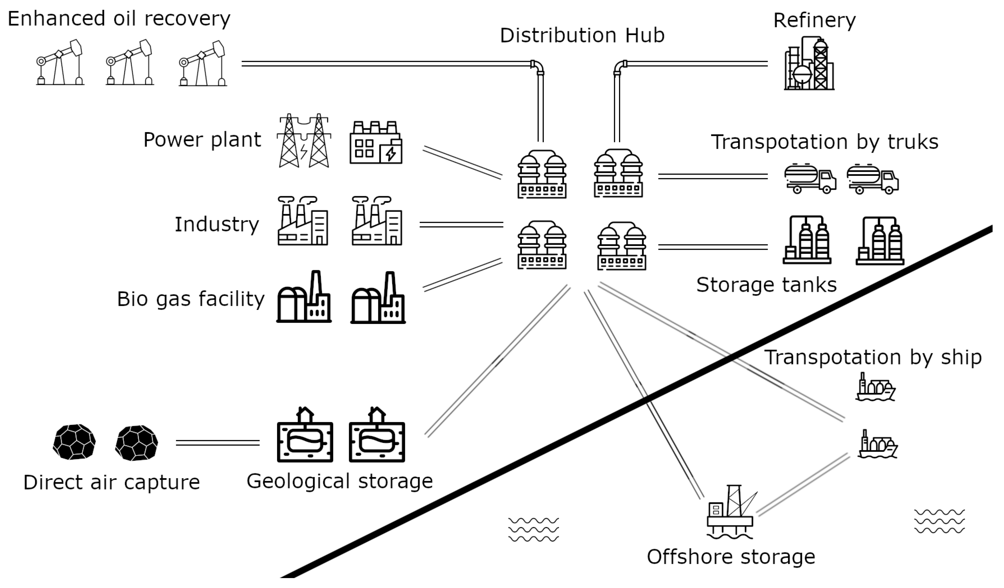
Schematic representation of a CCUS system. The figure illustrates the interconnected components and pathways involved in capturing CO2 from various sources, its transportation and subsequent utilisation or storage. This holistic view highlights key processes such as carbon capture, transportation and both onshore and offshore storage, demonstrating the complexity and integration required for effective carbon management within a CCUS network.
Figure 1.
Schematic representation of a CCUS system. The figure illustrates the interconnected components and pathways involved in capturing CO2 from various sources, its transportation and subsequent utilisation or storage. This holistic view highlights key processes such as carbon capture, transportation and both onshore and offshore storage, demonstrating the complexity and integration required for effective carbon management within a CCUS network.
The aim of the directive is to establish a legal framework for environmentally safe geological storage of CO2. This is done by outlining the procedures for obtaining permits for the operation of CCS facilities. These procedures include submitting an application to the EU member state hosting the facility. Such an application should include the following points:
- The name and address of the potential operator
- Proof of the technical competence of the potential operator
- The characterisation of the storage site and complex and an assessment of the expected security of the storage
- The total quantity of CO2 to be injected and stored, as well as the prospective sources and transport methods, the composition of CO2 streams, the injection rates and pressures and the location of injection facilities
- A description of measures to prevent significant irregularities
- A proposed monitoring plan
- A proposed corrective measures plan
- A proposed provisional post-closure plan
The directive further describes how the monitoring of the CCS facility (including the injection points and the storage complex until where possibly the CO2 plume can reach the surrounding environment) is the responsibility of the operator and should include the following points:
- Comparing between the actual and modelled behaviour of CO2 in the storage site
- Detecting significant irregularities
- Detecting migration of CO2
- Detecting leakage of CO2
- Detecting significant adverse effects for the surrounding environment, including in particular on drinking water, for human populations or for users of the surrounding biosphere
- Assessing the effectiveness of any corrective measures taken in case of leakages or significant irregularities
- Updating the assessment of the safety and integrity of the storage complex in the short and long term, including the assessment of whether the stored CO2 will be completely and permanently contained
Figure 2.
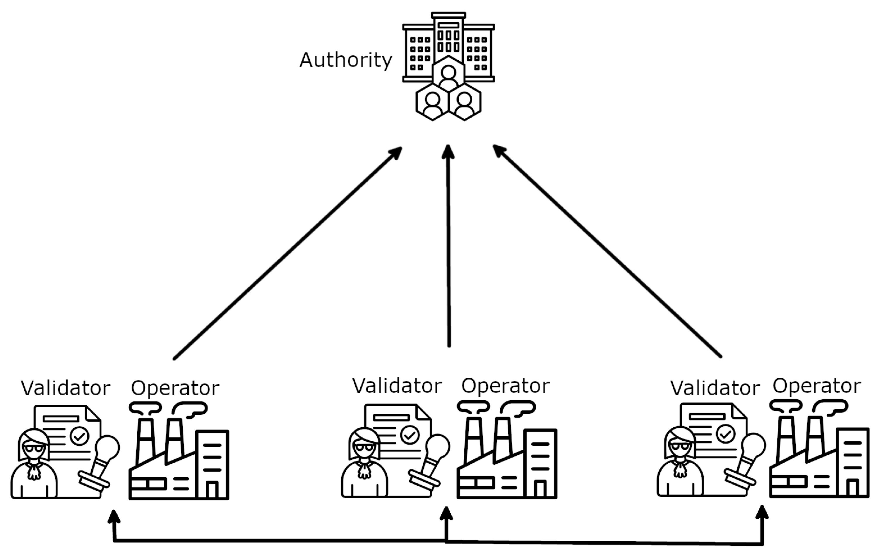
Schematic representation of the carbon emission trading process. The figure illustrates the roles and interactions between key stakeholders, including the regulatory authority, validators and operators. The authority oversees the trading framework, while the validators ensure the accuracy and compliance of reported emissions. Operators participate in the trading system by buying and selling emission allowances, adhering to the established rules and ensuring proper verification by the validators. This process showcases the flow of information and accountability within the carbon trading system.
Figure 2.
Schematic representation of the carbon emission trading process. The figure illustrates the roles and interactions between key stakeholders, including the regulatory authority, validators and operators. The authority oversees the trading framework, while the validators ensure the accuracy and compliance of reported emissions. Operators participate in the trading system by buying and selling emission allowances, adhering to the established rules and ensuring proper verification by the validators. This process showcases the flow of information and accountability within the carbon trading system.
The main problem with this description and with the EU CCS directive in general is that is does not provide any indication of how small leakages or irregularities must to be detected as part of the monitoring program. In Section 5, we provide an review of how small leakages are realistic to detect.
2.2. Requirements for Carbon Emission Trading
At the time of writing there exist in the world 6 operating carbon trading systems:
- The European Union Emissions Trading System (EU ETS)
- The California Cap-and-Trade Program
- The Regional Greenhouse Gas Initiative (RGGI)
- The China’s National Emissions Trading System (ETS)
- The New Zealand Emissions Trading Scheme
- The South Korea Emissions Trading Scheme
Here we will focus on the EU ETS, which is the largest carbon trading system globally, established in 2005.
Operating on a cap-and-trade principle, the EU sets a limit or ("cap") on the total greenhouse gas emissions permitted from energy-intensive sectors like power generation, manufacturing and aviation. Companies within the system receive emissions allowances, each representing the right to emit one ton of CO2 or its equivalent. These allowances can be freely allocated or auctioned by governments. Participants must surrender enough allowances at the end of each compliance period to cover their actual emissions. Failure to do so results in significant penalties.
Trading of allowances occurs among companies, enabling those needing more allowances to purchase them from others who have a surplus, establishing a market where prices are determined by the balance of supply and demand. Presently, EU ETS does not permit the acquisition of carbon credits from sinks, such as tree planting initiatives aimed at reducing CO2 levels. The reason for this is linked to the difficulty of monitoring, measuring and verifying the effective removal capacity of such sinks.
The EU Monitoring and Reporting Regulation (MRR) outlines the requirements for monitoring and reporting GHG emissions. Under this framework, facilities can choose between a "Calculation approach for CO2" or a "Measurement approach for CO2." The measurement approach allows for the use of Continuous Emission Monitoring Systems (CEMS), which are particularly applicable to CCUS facilities. The required precision levels for CEMS are specified in Annex VIII of the EU Monitoring and Reporting Regulation No. 2018/2066.

Table 1.
Tiers for CEMS (maximum permissible uncertainty for each tier)
| Tier 1 | Tier 2 | Tier 3 | Tier 4 |
|---|---|---|---|
| ±10% | ±7.5% | ± 5% | ± 2.5% |
where the term "Tier" refers to different levels of methodologies or approaches used to estimate emissions. Category A installations, which are high-emission and energy-intensive industrial installations here need to apply to minimum Tier 2.
It is thus clear that the requirements for carbon emission trading are much more concrete than the requirements from legislation for CCUS. It must however, be expected that the uncertainty requirements for CEMS will be adopted by the legislation requirements for CCUS in the future.
3. Observations methods
In 2020 the IEA GHG made a review of the monitoring technologies in CO2 storage including 43 technologies, which they divided into three main categories: atmospheric, surface/near-surface and reservoir zone. The study suggested that the majority (55%) of the monitoring technologies concerns the reservoir zone. The reason for this could be that the reservoir zone is the focus of the oil and gas operators attempting to maximize recovery in hydrocarbon fields [12] and therefore receives significant attention and investments.
The QUEST project [13] has implemented a risk-based MVA plan for containment and conformance, which has been refined over the years through lessons learned during its implementation phases. A crucial element of this CCS monitoring plan was the ranking of technologies based on their lifecycle cost-benefit estimates, derived from the identified monitoring tasks. Technologies with higher ranking values are considered more beneficial and less costly, while those with lower ranking values are on the contrary seen as less beneficial and more costly. The total benefit of each monitoring technology was estimated by the number of monitoring tasks they could perform, weighted by the likelihood of their success. Among the top eight technologies were well-head CO2 detectors, satellite or airborne hyperspectral image analysis and Interferometric Synthetic Aperture Radar (InSAR) monitoring. Conversely, the bottom eight technologies were all related to well logging, so even though reservoir zone monitoring technologies are the most popular, they do not seem to be the most cost efficient [13].
While studying the reservoir zone can yield valuable insights into the structure and dynamics of the reservoir, it does not offer information on potential leakage, which is the focus of this study. Therefore, we will concentrate on atmospheric and surface/near-surface technologies. These technologies are categorized into:
Table 2.
GHG observation methods
| Detection limit | Precision | Coverage | ||||
|---|---|---|---|---|---|---|
| CO2 | Methane | CO2 | Methane | |||
| In situ | ||||||
| NDIR sensors | 1-5 ppm | 10-50 ppm | ∼2% | ∼2% | 1–2 sec. | |
| Photoacoustic sensors | 1 ppm | 1–10 ppb | ∼1% | ∼1% | <1 sec. | |
| TDLAS sensors | 0.1–1 ppm | 1-10 ppb | 0.1% | 0.1% | <1 msec. | |
| Drones | ||||||
| Sniffer sensors | 1–3 ppm | 1-80 ppb | 2% | 2% | 1–2 sec. | |
| Thermal inferred imaging | ∼5 ppm | ∼10 ppm | 2% | 2% | <100 msec. | |
| Hyperspectral imaging | 1–10 ppm | 1–10 ppm | 1% | 1% | <1 sec. | |
| LIDAR | 1–10 ppm | 1-10 ppm | 1% | 1% | <1 sec. | |
| Satellites | ||||||
| Spectroscopic sensors | 1–4 ppm | 10-50 ppb | 1-2 ppm | 10–20 ppb | 1–3 days | |
| Interferometry | - | ∼100 ppb | - | 10-20 ppb | 1–2 weeks | |
| LIDAR | 1–2 ppm | 10-50 ppb | 1 ppm | 10 ppb | 1–7 days | |
3.1. In Situ
In situ measurements of GHGs are performed by placing a sensor close to the emission source. The most common kinds of GHG sensors are:
3.1.1. Non-Dispersive Infrared sensors
Non-Dispersive Infrared (NDIR) sensors work by measuring the absorption of infrared radiation by specific gases. These sensors contain an infrared light source, a gas sample chamber and a detector. When infrared light passes through the gas sample, the target molecules absorb specific wavelengths of infrared light. By measuring the decrease in infrared light intensity, the sensor can determine the concentration of the target gas.
3.1.2. Photoacoustic sensors
Photoacoustic sensors are based on the photoacoustic effect, where the absorption of light with a specific wavelength by a gas sample leads to the generation of acoustic waves. The waves are detected by an highly sensitive microphone and by analyzing the amplitude of the acoustic signal, the sensor can determine the concentration fo the target gas.
3.1.3. Tunable Diode Laser Absorption Spectroscopy
Tunable Diode Laser Absorption Spectroscopy (TDLAS) sensors use a tunable diode laser to emit light at highly specific wavelengths corresponding to the absorption bands of the target compounds. The interaction between the emitted light and the gas sample is then measured to determine the gas concentration. The high intensity and monochromacy of laser light makes TDLAS sensors able to offer high sensitivity, making them the preferred choice, where high precision is required.
A specific kind of in situ measurements are made using flux towers, where one or more GHG sensors are placed in a tall tower along with a suite of methodological instruments. By combining the measured concentrations with methodological data it is possible to measure the GHG flux at the location of the tower. Such kind of measurements are important both for modelling large scale GHG transportation and calibrating satellite observations [14].
3.2. Drones
When mounting sensors on drones for measuring GHG concentrations, several factors need specific consideration, including weight, power consumption, size, accuracy and response time, but in general the same sensors that are used for in situ measurements can be mounted on a drone.
Additionally, as a drone is monitoring a facility from a distance, imaging techniques can also be advantageously utilised here.
The drone-based solutions include:
3.2.1. Sniffer Sensors
Drones can combine a gas sensor (such as NDIR, photoacoustic or TDLAS sensors) with formation flying to produce images of GHG concentrations and measure point sources of emissions. One specific approach is the tracer gas technique, where a known quantity of tracer gas is released into the environment. By measuring its concentration at various locations, it is possible to determine airflow patterns, detect leaks or quantify gas emissions [15]. While drones are particularly suited for this technique due to their ability to operate in three dimensions, tracers are a versatile method that can also be employed with in situ measurements (e.g., stationary sensors or mobile platforms like cars) or even theoretically with satellite observations, depending on the tracer gas properties and detection capabilities. However, car-based (and satellite-based) measurements typically involve higher uncertainties due to their limitation to two-dimensional movement compared to the three-dimensional flexibility of drones.
3.2.2. Thermal Infrared Imaging
Thermal infrared cameras can detect heat signatures and more generally acquire images in the infrared region of the spectrum associated with GHG emissions, such as those from industrial processes or natural gas leaks, i.e., where the absorption of GHGs is higher. This means that they can make emission plumes visible as a consequence of its different infrared light absorption properties and are consequently commonly used for detecting leaks in pipelines, storage tanks and industrial equipment.
3.2.3. Hyperspectral Imaging
Hyperspectral imaging systems capture imagery across multiple wavelengths, allowing for the detection of spectral signatures associated with GHG concentrations or related parameters. For example, hyperspectral imaging can be used to monitor vegetation health and detect changes in carbon storage in forests or agricultural lands. Additionally, infrared hyperspectral imaging can be employed to measure GHG concentrations by analyzing the absorption of specific infrared wavelengths by GHG molecules. This absorption is characteristic of each gas, allowing for precise detection and quantification of GHGs.
3.2.4. Light Detection and Ranging System
Light detection and ranging (LIDAR) systems emit laser pulses and measure the reflected light to create detailed 3D maps of terrain and vegetation structure. This technique can be used to quantify forest biomass and monitor carbon sequestration, as well as to detect emissions from industrial facilities or natural gas leaks, in conjunction with the absorption of laser light operated by the GHG molecules.
It must be pointed out that all the described techniques, whose effectiveness is boosted by the extreme mobility of drones can however, also be operated as stationary installations or be held by a person. This is especially the case for thermal infrared cameras, which are often used (and in some cases mandated by law) to monitoring leaks from oil and gas facilities by an operator that physically inspects the sections of the infrastructure that presents the higher risk.
3.3. Satellites
Satellite observations are based on spectroscopic, interferometric or LIDAR based methods:
3.3.1. Spectroscopic Sensors
Spectroscopic sensors measure the absorption or emission of electromagnetic radiation by gases or particles in the atmosphere. These methods utilize the unique spectral signatures of gases to identify them and quantify their concentrations, in the same way as the sensors described for in situ monitoring, but with the significant difference of remote detection. The observations can be based either on: push broom technique, where a slit spectrograph collects a 1D line of observations, which is converted into a 2D observations as the satellite move forward; or on the whisk broom technique, where the GHG concentrations in the atmosphere are measured one pixel at a time.
3.3.2. Interferometry
Interferometric techniques have the advantage that they can provide a 3D snapshort and do not have to rely on the push or whisk broom techniques. These techniques are generally categorized based on the type of interferometer they use. These are:
- Michelson interferometer, where the light is split into two different paths which leads to interference depending on the different path lengths.
- Fabry-Pérot interferometer, where the light undergoes multiple partial reflections between two mirrors leading to interference depending on the distance between the mirrors.
GHGSat, in particular, utilises a modified version of the Fabry-Pérot interferometer, where the distance between the mirrors remains constant, but the travel path of light between the mirrors varies depending on its origin within the image field. By scanning the image field for a specific ground location, the system sequentially measures the light received from different parts of the image field. This scanning process effectively changes the angle of incidence of the incoming light on the interferometer, which in turn influences the optical path length. As a result, different wavelengths of light are selectively transmitted or reflected at each scan position. This allows the system to capture spectral information across a range of wavelengths, providing detailed insights into the composition of gases over the scanned ground location.
3.3.3. LIDAR
LIDAR methods can detect the properties of the atmosphere, including aerosol concentrations, cloud heights and GHG gas concentrations, by measuring the time delay and intensity of laser pulses reflected or scattered back from atmospheric targets. An example of a satellite that uses the LIDAR method is MERLIN [21].
Figure 3.
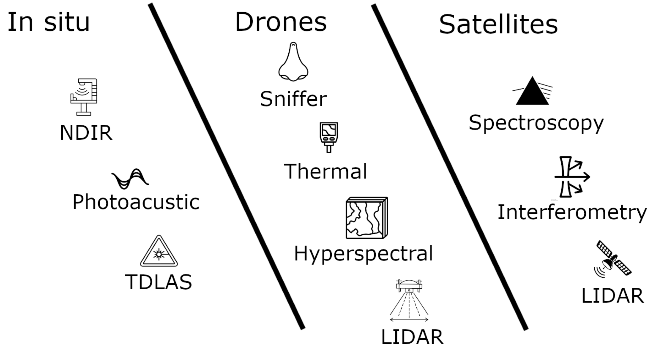
Overview of CCUS monitoring technologies, categorized by in-situ, drone-based and satellite-based platforms. The figure illustrates the range of technologies employed across these platforms to detect and quantify greenhouse gas emissions. Each platform offers distinct advantages in spatial and temporal coverage, providing complementary approaches for comprehensive monitoring within the CCUS system.
Figure 3.
Overview of CCUS monitoring technologies, categorized by in-situ, drone-based and satellite-based platforms. The figure illustrates the range of technologies employed across these platforms to detect and quantify greenhouse gas emissions. Each platform offers distinct advantages in spatial and temporal coverage, providing complementary approaches for comprehensive monitoring within the CCUS system.
4. Analysis Methods
All the measurement methods described above require preprocessing before they can provide a measured GHG concentration or flux. The preprocessing differs between in situ sensing and imaging methods. This process involves at least two steps. In the first step, retrieval algorithms are used to obtain a measured concentration. In the second step, a dispersion or transportation model converts this measured concentration into a GHG flux, considering the topography and wind field. Various types of observations can be used as input for these models through data assimilation algorithms.
4.1. Retrieval Algorithms
Retrieval algorithms process raw data from GHG measurement platforms to estimate concentrations accurately. The steps vary depending on whether the measurements are collected from in situ sensors, drones or satellites. Below is a structured breakdown of retrieval steps for each platform.
4.1.1. In Situ Sensors
For point-based measurements such as NDIR, photoacoustic and TDLAS, the retrieval steps are:
- 1.
- Calibration: Align the sensor to known standards and correct for baseline drift and noise.
- 2.
- Concentration calculation: Use models like the Beer-Lambert law to estimate gas concentrations based on signal properties or absorption spectra.
- 3.
- Environmental corrections: Account for external factors like temperature and pressure to improve accuracy.
4.1.2. Drone-Based Techniques
Drones enable spatially resolved measurements using various advanced sensors. The general retrieval steps for drone-based techniques are:
- 1.
- Preprocessing: Remove sensor noise, correct for atmospheric effects and calibrate raw data for accuracy.
- 2.
-
Feature extraction:
- -
- For sniffer sensors, detect concentration peaks at point sources.
- -
- For imaging techniques (thermal infrared or hyperspectral), identify spectral or radiometric features associated with GHGs.
- 3.
- Concentration mapping: Combine spatial and spectral data to estimate GHG concentrations across a defined area, incorporating corrections for environmental factors like surface emissivity (thermal) or spectral unmixing (hyperspectral).
- 4.
- Validation: Compare drone-based retrievals with ground-based measurements or simulations for quality assurance.
4.1.3. Satellite-Based Observations
Satellites measure column-averaged GHG concentrations and require more complex retrieval processes to account for atmospheric and surface effects:
- 1.
- 2.
- Albedo Corrections: Adjust for biases caused by surface reflectance to ensure accurate retrievals [23].
- 3.
- GHG concentration estimation: Derive GHG concentrations using mathematical inversion techniques that relate the observed spectra to gas properties.
- 4.
- Validation: Cross-verify satellite retrievals with ground-based or airborne measurements to assess accuracy and identify systematic biases.
4.2. Emission Estimation
The retrieval algorithms enable the measurement of GHG concentrations at different spatial scales depending on the sensor type. For in situ sensors, the concentration is measured either within the sensor or along the laser’s line-of-sight. For thermal infrared cameras and LIDAR devices, the concentration is determined along the line-of-sight. For satellite observations, the retrieval provides the mean concentration within the air column. In most cases however, these concentrations are not the important parameter to estimate. Instead, we are most often interested in knowing the GHG emission from a given geographical location or region. These quantities are estimated from the measured concentration using inversion methods that compare the observation with a theoretical model through the following formula:
where y are the observations and x are the parameters that we want to estimate, called the state vector. Most often (even though not always) x will be the GHG fluxes, while is an error term. The measured concentration is related to the state vector through what is called the forward model , which in our case is a Chemical Transportation Model [CTM, [25]. This is done by using an inversion method, of which there exist a few.
4.2.1. Chemical Transport Models
CTMs can be separated into the following three categories:
- Eulerian models
- Lagrangian models
- Plume models
Eulerian models calculate the velocity, pressure and GHG concentrations at a set of points defined on a grid, while the frame of reference in the Lagrangian models follows the particles. The plume models on the other hand assume that the dispersion of gases in the atmosphere can be approximated by a Gaussian distribution.
Eulerian models
Eulerian CTMs focus on the movement of gasses from their sources to various receptor locations, considering the pathways and mechanisms through which gasses are transported through the atmosphere. These models take into account factors such as emission sources, emission rates, transportation pathways (e.g., atmospheric currents, transport networks) and deposition processes (e.g., dry deposition, wet deposition). Eulerian CTMs are used to estimate the spatial and temporal distribution of gases over larger geographic areas, including regional and global scales. Examples of Eulerians CTMs are WRF-Chem [26] and GEOS-Chem [27]
Lagrangian models
Lagrangian CTMs use a different approach compared to Eulerian models. Instead of dividing the atmosphere into a grid and tracking gasses concentrations within each grid cell, Lagrangian CTMs follow the movement of individual air parcels or particles as they transport pollutants through the atmosphere.
Lagrangian CTMs can be run both forward and backward in time. In the forward case, particles are released from one or more sources and collected again at a number of different receptors. An example for a forward Lagrangian CTM is FLEXPART [28] In the backward case, particles are released at the receptors and time is then run backward to follow the particles back to their sources. Backward Lagrangian CTMs are particular useful for calculating influence function or the footprints as described below. An example for a backward Lagrangian CTM is the Stochastic Time-Inverted Lagrangian Transport model STILT [29]
Plume models
Plume models are used to predict the dispersion of gases emitted from point sources into the atmosphere, such as chimneys or power plants. These models are particularly useful under conditions of atmospheric stability and rely on the assumption that gas dispersion follows a Gaussian distribution. They account for factors such as wind speed, wind direction, atmospheric stability and turbulence to simulate how pollutants spread downwind from their emission source. By modeling the dispersion process, plume models estimate pollutant concentrations at various locations, providing valuable insights for assessing air quality and understanding pollutant behavior [30].
4.2.2. Inversion Methods
In general, GHG inversion methods can be separated into the following three categories:
- Bayesian inversion
- Data assimilation
- Influence function-based inversion
Bayesian inversion analysis
The main task of the inversion analysis is to find the most optimal set of input parameters for a forward model that best matches the observations. This is almost always done in a Bayesian framework, where the input parameters, i.e. the state vector, that provides the highest posterior probability, are selected.
When performing a simple Bayesian inversion, the state vector most often contains the GHG fluxes, which are estimated by minimising the Bayesian cost function [31]:
where is the state vector, is the prior state vector, is the prior covariance matrix and is the covariance matrix.
This cost function can be minimized by assuming that the forward model is linear so that the forward model can be expressed as function of the Jacobian matrix :
where
If the assumption that the forward model is linear is valid, the Jacobian matrix can be constructed by perturbing the elements in the state vector one at a time and monitor the effect on . An example for how GHG emission can be calculated using a Bayesian inversion analysis is provided in Varon et al. [32].
Data assimilation
If the forward model is not linear with respect to the state vector , then the Jacobian matrix is not independent of the state vector and must therefore be recalculated whenever the state vector is updated. If the state vector is large, this becomes too heavy from a computational point of view.
The solution to this, offered by data assimilation approach, is to calculate the gradient of the cost function for successive guesses of the state vector and so using a descent algorithm to directly minimize the cost function .
One of the most common examples (and thus a classic case of when data assimilation is useful) of the state vector being too large for allowing the calculation of the Jacobian matrix is when the state vector contains GHG concentrations and not emissions and this is thus a classical example of when data assimilation is used. This does not however, have to be the case for data assimilation to be the right inversion method - as long as the forward model is not linear and the state vector is large. An example for how GHG emission can be calculated using data assimilation is provided in Meirink et al. [33].
Influence function-based inversion
If the observations are sparse and the state vector is large, it makes sense to calculate the influence function or the footprint for each observation. This parameter is also referred to as the adjoint sensitivity and is in fact the transpose of the Jacobian matrix .
In this approach, the forward model is only used to calculate the Jacobian matrix and not to minimise the cost function . An example of how GHG emission can be calculated using influence function based inversion is provided in Wu et al. [34]
4.3. Carbon Budgets
Carbon budgets play a crucial role in national inventories of GHG emissions and removals. National inventories are comprehensive assessments of a country’s emissions and removals of GHGs, including carbon dioxide, methane, nitrous oxide and chlorofluorocarbon (CFC) gases. These inventories are used for tracking the progress towards international climate commitments, such as those under the United Nations Framework Convention on Climate Change (UNFCCC) and the Paris Agreement.
The UNFCCC recommends that national inventories are validated using both a bottom-up and a top-down approach [35,36].
In the bottom-up approach the national inventories should be compared to independently compiled estimates such as for example the Emission Database for Global Atmospheric Research [EDGAR, [37]), which is a comprehensive database providing global estimates of greenhouse gas and air pollutant emissions developed by the European Commission’s Joint Research Centre (JRC). EDGAR collects and compiles data on emissions from various sources, including industrial activities, energy production, transportation, agriculture, and waste management. It covers a wide range of pollutants, including carbon dioxide (CO2), methane (CH4), nitrous oxide (N2O), sulfur dioxide (SO2), nitrogen oxides (NOx), volatile organic compounds (VOCs) and particulate matter.
In the top-down approach the national inventories should be instead compared to atmospheric measurements. UNFCCC provides guidance on how inverse modeling should be used to provide emission estimates. The guide mainly focuses on satellite observations and suggests including the following steps in a validation of national inventories:
- Acquisition of observations
- Preparation of gridded prior emission data
- Operation of the inverse model
- Quality assurance and control of the inverse model output
- Comparison, verification and reporting
A critical aspect of accurately quantifying total GHG emissions is considering biogenic contributions, which represent a substantial component of the overall carbon budget. Biogenic emissions, derived from natural sources such as wetlands, forests and soil microbial activity, can significantly influence regional and national emission estimates. Incorporating models and inventories that account for these biogenic emissions can improve the alignment of calculated emissions with observational data, thereby enhancing the validation process of national inventories.
Specifically, integrating biogenic contributions involves using models that simulate natural processes and emissions. For example, dynamic global vegetation models or land surface models could be utilized to account for biogenic carbon fluxes. These models provide spatially explicit data, complementing satellite-based observations and atmospheric inversions used in top-down approaches. Moreover, combining such models with land-use inventories could aid in distinguishing anthropogenic emissions from natural variability, ultimately refining the overall accuracy of national GHG inventories.
UNFCCC provides examples of how this has been done in Switzerland, the UK and Australia, but in general very few countries have as per today used a top-down approach for validating their national inventories.
The Global Carbon Project publishes an annual global carbon budget annually [38] and a global methane budget [6], where a number of inventories are compared to results from inversion of concentration measurements. The inventories that are used in these studies include, among others, the data set from the United States Environmental Protection Agency [USEPA, [39], the Greenhouse gas and Air pollutant INteractions and Synergies (GAINS) model, the Emissions Database for Global Atmospheric Research (EDGAR) and the Community Emissions Data System [CEDS, [40]), which are compared to a number of atmospheric inversion estimates based on both in situ observations and observations from the GOSAT and OCO-2 satellites.
For the carbon budget, 13 inversion models were compared to the bottom-up or bookkeeping results and close agreement were found between the net ocean and land carbon sinks and the top-down approach obtained from atmospheric inversion of GOSAT and OCO-2 observation for the period 2013-2022 [38].
For the global methane budget [6], 22 inversion models were compared to the bottom-up results, but in this case a discrepancy as big as +30% was found with the top-down approach obtained from atmospheric inversion of GOSAT observations for the period 2008-2017. The cause is still not exactly understood, but errors related to up-scaling local measurements and double counting of some natural sources are suggested as the source [6].
5. Discussions
An optimal GHG monitoring system for CCUS should combine bookkeeping methods with direct measurements to achieve a comprehensive understanding of emissions. However, there is generally a lack of precise requirements for such systems, which poses challenges for consistent and accurate monitoring. A practical starting point could be adopting the MRR CEMS Tier 1 requirement, which mandates a precision better than 10%. This precision benchmark provides a foundation for developing more detailed guidelines, but it still leaves several critical aspects unaddressed. For instance, there is a notable lack of guidelines regarding the permissible magnitude of GHG leaks from CCUS facilities. This is partly due to the diverse nature of different CCUS facilities, such as EOR, DAC and BECCS, each of which presents unique monitoring challenges. Many regulatory frameworks, such as the EU CCS directive, aim for zero leakage, but in practice it may be more sensible to refer to zero measurable leakage, clearly defining what is considered as measurable. This nuanced approach would acknowledge the limitations of current technology while setting realistic goals for emission reduction.
As shown in Table 2, several techniques exist that allow the detection of CO2 concentrations as low as 1-10 ppm and methane concentrations as low as 1-10 ppb. However, converting these concentrations into emission levels is generally not feasible, as the impact varies significantly depending on whether the emission occurs locally (e.g., at the injection point) or is fugitive over a large area (e.g., from a large geological storage site). One exception here is observations preformed using the tracer gas technique, where detection limits of 5-25 kg/h and 0.2-0.5 kg/h, depending on the wind speed and distance to the source, can be obtained for CO2 and methane, respectively. We suggest to overcome these limitations by defining measurable leakage in terms of the increase in concentration it causes, rather than the emission rate itself. By adopting background levels of 420 ppm for CO2 and 1900 ppb for methane (as per 2024 according to the National Oceanic and Atmospheric Administration) and applying the 10% precision requirement from the MRR CEMS Tier 1 with a detection limit, we arrive at threshold levels of 588 ppm and 2660 ppb for CO2 and methane, respectively. These levels would need to be adjusted to account for background levels that change with time and location. Such threshold levels stems from the assumption of zero emissions and therefore, if some emissions are permitted, they thresholds could be accordingly increased.
The threshold levels provided above do not account for natural variability in the background levels. Generally, the natural variability is well below 10%, except in specific areas, such as urban regions. For areas with elevated background levels or large natural variability, the threshold values should be adjusted accordingly. This adjustment is crucial, as it ensures that the monitoring system remains sensitive enough to detect real leaks without being overwhelmed by natural fluctuations and becoming consequently unreliable. While it might be relatively straightforward for a geological CCS site to remain within these thresholds, it will likely be more challenging for BECCS sites, as biogas production facilities are known to be associated with significant methane leakage. Setting the final threshold levels will ultimately be a political decision, but it is crucial to ensure that the limits set guarantee a net negative GHG emission.
Transitioning from an emission-based to a concentration-based GHG monitoring system would naturally favor data assimilation inversion systems, as a state vector containing GHG concentrations is generally larger than one containing emissions. However, it does not preclude the use of other types of inversion methods. On the contrary, the flexibility to choose the most appropriate inversion method depending on the specific characteristics of the CCUS facility and the available data is vital. This approach would in fact ensure that the monitoring system can adapt to different conditions and provide accurate, actionable insights.
An optimal GHG monitoring system should be designed to detect concentrations down to the threshold level with a precision better than 10% in and around the CCUS site. This should involve integrating all relevant data sources, including in-situ, drone and satellite measurements. While in-situ measurements would provide high precision and cadence, satellite observations would offer extensive spatial coverage, complemented by drone measurements. The integration of these diverse data sources is essential for creating a comprehensive monitoring system that can cover both the micro and macro scales of GHG emissions. The current legislation mandates that each drone must be operated by a human pilot, which limits their potential. However, in the future, autonomous drones are likely to be permitted. These autonomous drones could significantly enhance this field by providing high precision, spatial resolution and cadence, along with extensive spatial coverage. This technological advancement could be a game-changer for CCUS monitoring, enabling continuous and highly detailed surveillance of emissions at a fraction of the cost that would be required today.
These different observations would be combined in a data assimilation or another inversion tool. This way, it would not be the measurements directly that would be used to evaluate if the threshold level was violated, but the posterior from the inversion method. This approach would also minimize the risk of random noise sources causing false alarm threshold violation alerts. The use of advanced data processing techniques would ensure that the monitoring system remains robust, even in the face of complex and noisy data.
If the aggregated model triggers a threshold violation alarm, the operator of the CCUS facility should adopt a mitigation plan. The first step would be to identify the source of the elevated GHG levels. Here, the aggregated model could also assist, as it would contain model emission levels. Although the spatial resolution of these emission levels might be low, they would provide a first guess of where to look for significant leakages. This capability is crucial for enabling rapid and effective responses to any detected leaks, thereby minimizing their environmental impact. The development of such mitigation plans should be an integral part of the design and operation of CCUS facilities, ensuring that they can promptly and effectively respond effectively to any issues that arise.
In conclusion, the establishment of precise monitoring requirements and the integration of advanced measurement technologies are essential steps toward ensuring the effectiveness of CCUS systems. By adopting a concentration-based approach and leveraging the full range of available measurement tools, it is possible to create a monitoring system that is both comprehensive and adaptable. This system would not only ensure compliance with regulatory requirements but also contribute to the broader goal of reducing global carbon emissions. The future of CCUS monitoring lies in the continuous improvement of these systems, guided by ongoing research, technological development and the definition of robust regulatory frameworks.
6. Summary
This paper has explored the critical role of monitoring and verification in ensuring the effectiveness of CCUS technologies in mitigating GHG emissions. We have highlighted the limitations of current monitoring methods, particularly the reliance on bookkeeping approaches and advocated for the integration of direct measurement techniques, including in-situ monitoring, drones and satellite observations. These types of data collection platforms, when combined with advanced data assimilation and inversion techniques, offer a more accurate and comprehensive approach for monitoring GHG fugitive emissions from CCUS facilities.
The discussion emphasized the need for more specific regulatory requirements, including clear detection thresholds for emissions, to ensure that CCUS facilities achieve their intended environmental benefits. We proposed a concentration-based monitoring system as a practical solution to the challenges posed by the diverse nature of CCUS operations and we underscored the importance of integrating various observation methods to enhance the precision and coverage of GHG monitoring.
Ultimately, the success of CCUS technologies in contributing to global climate goals will depend on the implementation of robust and flexible monitoring frameworks that can adapt to technological advancements and ensure that all emissions, regardless of their scale, are accurately accounted for and mitigated. This paper provides a roadmap for developing such frameworks, offering insights into best practices for monitoring and reporting GHG emissions from CCUS facilities.
Acknowledgments
The work was supported by the Innovation Found Denmark through a grant to the MONICO project which is part of the INNO-CCUS Partnership.
Conflicts of Interest
The authors declare no conflicts of interest.
References
- United Nations Framework Convention on Climate Change. Paris Agreement 2015.
- Ketzer, J.M.; Iglesias, R.S.; Einloft, S. Reducing Greenhouse Gas Emissions with CO2 Captureand Geological Storage. In Handbook of Climate Change Mitigation; Chen, W.Y., Seiner, J., Suzuki, T., Lackner, M., Eds.; Springer US: New York, NY, 2012; pp. 1405–1440. [Google Scholar] [CrossRef]
- Sodiq, A.; Abdullatif, Y.; Aissa, B.; Ostovar, A.; Nassar, N.; El-Naas, M.; Amhamed, A. A review on progress made in direct air capture of CO2. Environmental Technology & Innovation 2023, 29, 102991. [Google Scholar] [CrossRef]
- Davoodi, S.; Al-Shargabi, M.; Wood, D.A.; Mehrad, M.; Rukavishnikov, V.S. Carbon dioxide sequestration through enhanced oil recovery: A review of storage mechanisms and technological applications. Fuel 2024, 366, 131313. [Google Scholar] [CrossRef]
- McLaughlin, H.; Littlefield, A.A.; Menefee, M.; Kinzer, A.; Hull, T.; Sovacool, B.K.; Bazilian, M.D.; Kim, J.; Griffiths, S. Carbon capture utilization and storage in review: Sociotechnical implications for a carbon reliant world. Renewable and Sustainable Energy Reviews 2023, 177, 113215. [Google Scholar] [CrossRef]
- Saunois, M.; Stavert, A.R.; Poulter, B.; Bousquet, P.; Canadell, J.G.; Jackson, R.B.; Raymond, P.A.; Dlugokencky, E.J.; Houweling, S.; Patra, P.K.; et al. The Global Methane Budget 2000–2017. Earth System Science Data 2020, 12, 1561–1623. [Google Scholar] [CrossRef]
- Vara-Vela, A.L.; Rojas Benavente, N.; Nielsen, O.K.; Nascimento, J.P.; Alves, R.; Gavidia-Calderon, M.; Karoff, C. Quantifying Methane Emissions Using Satellite Data: Application of the Integrated Methane Inversion (IMI) Model to Assess Danish Emissions. Remote Sensing 2024, 16. [Google Scholar] [CrossRef]
- Yver-Kwok, C.; Philippon, C.; Bergamaschi, P.; Biermann, T.; Calzolari, F.; Chen, H.; Conil, S.; Cristofanelli, P.; Delmotte, M.; Hatakka, J.; et al. Evaluation and optimization of ICOS atmosphere station data as part of the labeling process. Atmospheric Measurement Techniques 2021, 14, 89–116. [Google Scholar] [CrossRef]
- Boesch, H.; Liu, Y.; Tamminen, J.; Yang, D.; Palmer, P.I.; Lindqvist, H.; Cai, Z.; Che, K.; Di Noia, A.; Feng, L.; et al. Monitoring Greenhouse Gases from Space. Remote Sensing 2021, 13. [Google Scholar] [CrossRef]
- IEA. Tracking Clean Energy Progress 2023. 2023. Available online: https://www.iea.org/reports/tracking-clean-energy-progress-2023.
- Havercroft, I. CCS LEGAL AND REGULATORY INDICATOR. The Global CCS Institute 2018. [Google Scholar]
- Gupta, N.; Ravi-Ganesh, P.; Sminchak, J.R.; Conner, A.; Burchwell, A.; Place, M.; Kelly, M. Monitoring and Modelling of CO2 Storage: The Potential for Improving the Cost-Benefit Ratio of Reducing Risk. IEAGHG Technical Report 2020-01, 2020. [Google Scholar]
- Shell. Quest Carbon Storage and Capture Project: Appendix A – Monitoring, Measurement, and Verification Plan. Shell Canada Limited, 2010.
- Herig Coimbra, P.H.; Loubet, B.; Laurent, O.; Bignotti, L.; Lozano, M.; Ramonet, M. Eddy covariance with slow-response greenhouse gas analysers on tall towers: bridging atmospheric and ecosystem greenhouse gas networks. Atmospheric Measurement Techniques 2024, 17, 6625–6645. [Google Scholar] [CrossRef]
- Lamb, B.K.; McManus, J.B.; Shorter, J.H.; Kolb, C.E.; Mosher, B.; Harriss, R.C.; Allwine, E.; Blaha, D.; Howard, T.; Guenther, A.; et al. Development of Atmospheric Tracer Methods To Measure Methane Emissions from Natural Gas Facilities and Urban Areas. Environmental Science & Technology 1995, 29, 1468–1479. [Google Scholar] [CrossRef] [PubMed]
- Parker, R.J.; Webb, A.; Boesch, H.; Somkuti, P.; Barrio Guillo, R.; Di Noia, A.; Kalaitzi, N.; Anand, J.S.; Bergamaschi, P.; Chevallier, F.; et al. A decade of GOSAT Proxy satellite CH4 observations. Earth System Science Data 2020, 12, 3383–3412. [Google Scholar] [CrossRef]
- Eldering, A.; Wennberg, P.O.; Crisp, D.; Schimel, D.S.; Gunson, M.R.; Chatterjee, A.; Liu, J.; Schwandner, F.M.; Sun, Y.; O’Dell, C.W.; et al. The Orbiting Carbon Observatory-2 early science investigations of regional carbon dioxide fluxes. Science 2017, 358, eaam5745. [Google Scholar] [CrossRef]
- Veefkind, J.; Aben, I.; McMullan, K.; Förster, H.; de Vries, J.; Otter, G.; Claas, J.; Eskes, H.; de Haan, J.; Kleipool, Q.; et al. TROPOMI on the ESA Sentinel-5 Precursor: A GMES mission for global observations of the atmospheric composition for climate, air quality and ozone layer applications. Remote Sensing of Environment 2012, 120, 70–83, The Sentinel Missions-New Opportunities for Science. [Google Scholar] [CrossRef]
- Jervis, D.; McKeever, J.; Durak, B.O.A.; Sloan, J.J.; Gains, D.; Varon, D.J.; Ramier, A.; Strupler, M.; Tarrant, E. The GHGSat-D imaging spectrometer. Atmospheric Measurement Techniques 2021, 14, 2127–2140. [Google Scholar] [CrossRef]
- Tobin, D.; Holz, R.; Nagle, F.; Revercomb, H. Characterization of the Climate Absolute Radiance and Refractivity Observatory (CLARREO) ability to serve as an infrared satellite intercalibration reference. Journal of Geophysical Research: Atmospheres 2016, 121, 4258–4271. [Google Scholar] [CrossRef]
- Ehret, G.; Bousquet, P.; Pierangelo, C.; Alpers, M.; Millet, B.; Abshire, J.B.; Bovensmann, H.; Burrows, J.P.; Chevallier, F.; Ciais, P.; et al. MERLIN: A French-German Space Lidar Mission Dedicated to Atmospheric Methane. Remote Sensing 2017, 9. [Google Scholar] [CrossRef]
- Hu, H.; Hasekamp, O.; Butz, A.; Galli, A.; Landgraf, J.; Aan de Brugh, J.; Borsdorff, T.; Scheepmaker, R.; Aben, I. The operational methane retrieval algorithm for TROPOMI. Atmospheric Measurement Techniques 2016, 9, 5423–5440. [Google Scholar] [CrossRef]
- Lorente, A.; Borsdorff, T.; Butz, A.; Hasekamp, O.; aan de Brugh, J.; Schneider, A.; Wu, L.; Hase, F.; Kivi, R.; Wunch, D.; et al. Methane retrieved from TROPOMI: improvement of the data product and validation of the first 2 years of measurements. Atmospheric Measurement Techniques 2021, 14, 665–684. [Google Scholar] [CrossRef]
- Noël, S.; Reuter, M.; Buchwitz, M.; Borchardt, J.; Hilker, M.; Bovensmann, H.; Burrows, J.P.; Di Noia, A.; Suto, H.; Yoshida, Y.; et al. XCO2 retrieval for GOSAT and GOSAT-2 based on the FOCAL algorithm. Atmospheric Measurement Techniques 2021, 14, 3837–3869. [Google Scholar] [CrossRef]
- Brasseur, G.P.; Jacob, D.J. Modeling of Atmospheric Chemistry; Cambridge University Press, 2017.
- Grell, G.A.; Peckham, S.E.; Schmitz, R.; McKeen, S.A.; Frost, G.; Skamarock, W.C.; Eder, B. Fully coupled "online" chemistry within the WRF model. Atmospheric Environment 2005, 39, 6957–6975. [Google Scholar] [CrossRef]
- Bey, I.; Jacob, D.J.; Yantosca, R.M.; Logan, J.A.; Field, R.M.; Fiore, A.M.; Li, Q.; Liu, H.; Mickley, L.J.; Schultz, M.G. Global modeling of tropospheric chemistry with assimilated meteorology: Model description and evaluation. Journal of Geophysical Research: Atmospheres 2001, 106, 23073–23095. [Google Scholar] [CrossRef]
- Stohl, A.; Hittenberger, M.; Wotawa, G. Evaluation of dispersion and transport in the atmosphere. Journal of Geophysical Research: Atmospheres 2005, 110. [Google Scholar] [CrossRef]
- Lin, J.C.; Gerbig, C.; Wofsy, S.C.; Andrews, A.E.; Daube, B.C.; Davis, K.J. Stochastic time-inverted Lagrangian transport model (STILT): A model for simulating atmospheric tracer transport. Journal of Geophysical Research: Atmospheres 2003, 108. [Google Scholar] [CrossRef]
- Turner, D.B. Workbook of Atmospheric Dispersion Estimates: An Introduction to Dispersion Modeling; CRC Press, 1994.
- Tarantola, A. Inverse Problem Theory and Methods for Model Parameter Estimation; SIAM, 2005.
- Varon, D.J.; Jacob, D.J.; Sulprizio, M.; Estrada, L.A.; Downs, W.B.; Shen, L.; Hancock, S.E.; Nesser, H.; Qu, Z.; Penn, E.; et al. Integrated Methane Inversion (IMI 1.0): a user-friendly, cloud-based facility for inferring high-resolution methane emissions from TROPOMI satellite observations. Geoscientific Model Development 2022, 15, 5787–5805. [Google Scholar] [CrossRef]
- Meirink, J.F.; Bergamaschi, P.; Krol, M.C. Four-dimensional variational data assimilation for inverse modelling of atmospheric methane emissions: method and comparison with synthesis inversion. Atmospheric Chemistry and Physics 2008, 8, 6341–6353. [Google Scholar] [CrossRef]
- Wu, D.; Lin, J.C.; Fasoli, B.; Oda, T.; Ye, X.; Lauvaux, T.; Yang, E.G.; Kort, E.A. A Lagrangian approach towards extracting signals of urban CO2 emissions from satellite observations of atmospheric column CO2 (XCO2): X-Stochastic Time-Inverted Lagrangian Transport model (“X-STILT v1”). Geoscientific Model Development 2018, 11, 4843–4871. [Google Scholar] [CrossRef]
- Intergovernmental Panel on Climate Change (IPCC). IPCC Guidelines for National Greenhouse Gas Inventories, IPCC, 2006.
- Intergovernmental Panel on Climate Change (IPCC). 2019 Refinement to the 2006 IPCC Guidelines for National Greenhouse Gas Inventories, IPCC, 2019.
- Crippa, M.; Oreggioni, G.; Guizzardi, D.; Muntean, M.; Schaaf, E.; Lo Vullo, E.; Solazzo, E.; Monforti-Ferrario, F.; Olivier, J.G.J.; Vignati, E. EDGAR v5.0 Greenhouse Gas Emissions. 2020. [Google Scholar]
- Friedlingstein, P.; O’Sullivan, M.; Jones, M.W.; Andrew, R.M.; Bakker, D.C.E.; Hauck, J.; Landschützer, P.; Le Quéré, C.; Luijkx, I.T.; Peters, G.P.; et al. Global Carbon Budget 2023. Earth System Science Data 2023, 15, 5301–5369. [Google Scholar] [CrossRef]
- United States Environmental Protection Agency (EPA). Inventory of US Greenhouse Gas Emissions and Sinks: 1990-2019. EPA Publication no. 430-R-21-010, 2021.
- McDuffie, E.E.; Smith, S.J.; O’Rourke, P.; Tibrewal, K.; Venkataraman, C.; Marais, E.A.; Zheng, B.; Crippa, M.; Brauer, M.; Martin, R.V. A global anthropogenic emission inventory of atmospheric pollutants from sector- and fuel-specific sources (1970–2017): an application of the Community Emissions Data System (CEDS). Earth System Science Data 2020, 12, 3413–3442. [Google Scholar] [CrossRef]
Disclaimer/Publisher’s Note: The statements, opinions and data contained in all publications are solely those of the individual author(s) and contributor(s) and not of MDPI and/or the editor(s). MDPI and/or the editor(s) disclaim responsibility for any injury to people or property resulting from any ideas, methods, instructions or products referred to in the content. |
© 2025 by the authors. Licensee MDPI, Basel, Switzerland. This article is an open access article distributed under the terms and conditions of the Creative Commons Attribution (CC BY) license (http://creativecommons.org/licenses/by/4.0/).
Copyright: This open access article is published under a Creative Commons CC BY 4.0 license, which permit the free download, distribution, and reuse, provided that the author and preprint are cited in any reuse.


