1. Introduction
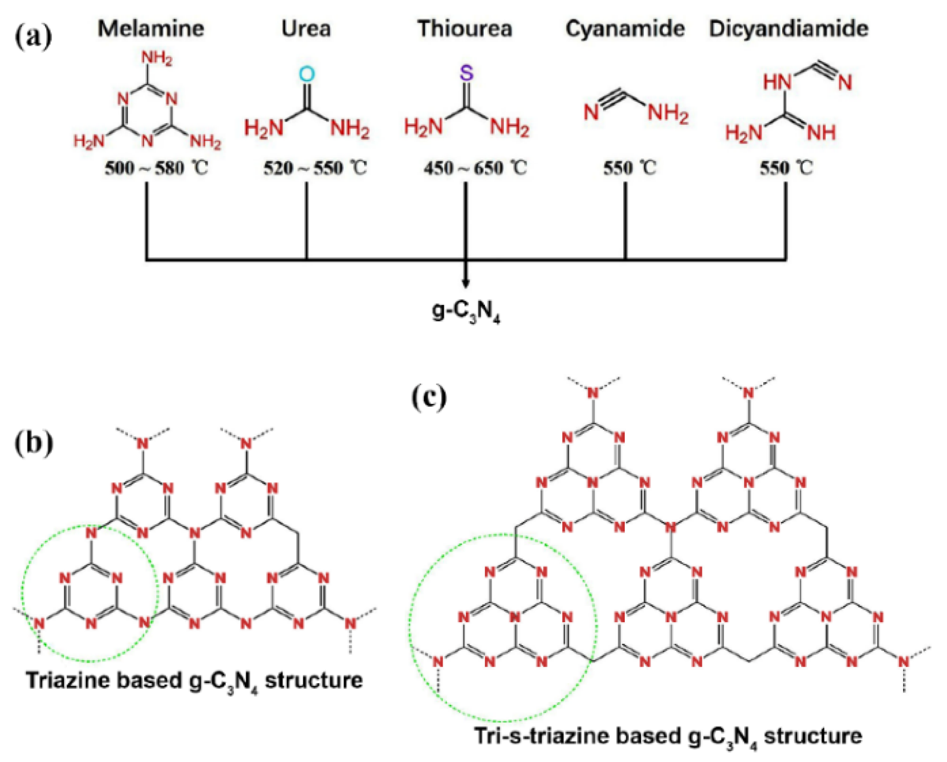
It is a substance that is prepared by thermal polycondensation at a temperature of 450-660°C [
1] from nitrogen-rich precursors with C-N core structure such as melamine, cyanamide, dicyandiamide, urea, thiourea; see scheme in
Figure 1.
With a graphite-like layered structure, g-C
3N
4 is in a form of 2D nanosheets, based on s-triazine or tri-s-triazine (
Figure 1) tectonic unit interconnected via tertiary amines [
2]. The presence of sp
2-hybridized C and N results in the unique g-C
3N
4, which plays a prime role in photocatalytic technologies, it is a highly active non-metallic photocatalyst [
3]. The photocatalytic activities of g-C
3N
4 are considerably affected by its structure, including its electronic structure. Both doping and composites are used for influence to obtain improved properties of new compounds, which then allow a wide range of possibilities for adaptive properties, e.g. for photocatalytic degradation, environmental remediation, removal of heavy metals from contaminated water, photocatalytic water splitting, photoreduction of CO
2, etc. Another factor is the influence of micro-, meso- and macro-pores in the fabric. Pore size influences water decomposition, production of H
2 and O
2, reduction of CO
2 (CH
3OH, CH
4). HARD-TEMPLATE METHOD, SOFT-TEMPLATE METHOD and TEMPLATE-FREE METHOD are also described. These methods modify the pore structure. g-C
3N
4 can be exfoliated chemically, mechanically and by ultrasound [
4,
5,
6]. An important application of g-C
3N
4 is in wastewater treatment by photo-oxidation reactions, where organic pollutants are degraded, bacteria are inactivated, and toxic heavy metals, antibiotics and a range of organic compounds are removed by photo-reduction reactions [
7,
8,
9,
10]. One of the other applications of g-C
3N
4 is membrane formation, which is used to trap pollutants, phenols, pharmaceutical products, organic dyes, and for desalination. g-C
3N
4 shows good photocatalytic activity under visible light [
11,
12,
13].
gC,N + hγ→C,N e-1+O2→°O
gC,N e-1 + H2O →°°OH
°°OH/°O + Pollutant → Degradation
Graphitic carbon nitride can be functionalized [
14] ̶ COOH, ̶ SO
3H, ̶ OH to affect the electrochemical and physicochemical properties by elemental doping, both non-metallic (S, O, B, Cl, F) and metallic (Fe, Ni, Pb, Ag, Au). Applications in supercapacitors, in photocatalytic water splitting, as a flame retardant, appear to be promising [
15,
16]. g-C
3N
4 is one of the photocatalysts with minimal toxicity, a chemically stable substance with efficient light absorption in the visible near-infrared region [
17,
18].
The aim of this article was to synthesize gC3N4 and its modifications with diverse materials and to implement these modifications within a composite framework with polymer materials. The synthesized products were subsequently subjected to FT-IR, SEM, and TGA analyses to facilitate comparative evaluation and further examination of their photocatalytic properties.
2. Materials and Methods
2.1. Materials
Chemicals:
Melamine – purity 99 %; CAS: 108-78-1; Sigma-Aldrich s.r.o.;
Low Density Polyethylene (LDPE) TYPE 100 BW Exxon Mobil;
Polyvinyl butyral (PVB), Mowital, Kuraray Europe GmnH; Germany;
Dopamine hydrochloride – PA; CAS: 62-31-7; Sigma-Aldrich s.r.o.;
Tris (hydroxymethyl) amino- methane; purity 99,8 %; Sigma-Aldrich s.r.o.; CAS: 77-86-1;
Iron oxide - nanoscale –purity 96 %; CAS:1309-37-1; Sigma-Aldrich s.r.o.;
Graphene oxide (GO)– preparation by Hummers’ method [
19];
Reduced graphene oxide (rGO) – reduced by ascorbic acid [
19];
Graphene oxide MEND (GO MEND) – provided by the Mendel University in Brno in suspension 2gL
-1 [
20];
2.2. Methods
-
FTIR spectroscopy (Nicolet iS20 FTIR Spectrometer: type of experiment: single reflection diamond ATR; sample preparation: solid samples measured directly, powdered samples ground into a fine powder; the spectra were not modified using any corrections; measurement conditions: the spectral resolution: 4 cm-1; the number of scans: 128; technical parameters of the device:
-detector: thermoelectrically cooled DTGS
-IR source: single-point IR ceramic
-laser: solid-state, temperature-controlled diode laser
-beamsplitter: KBr
-Spectral range: 7800 – 350 cm-1
-Omnic 9 software
SEM EDX spectroscopy: (Tescan Vega 4, Tescan Vega 3) with accelerating voltage was 15 ke.
Thermogravimetric analysis (STA 449 F3 JUPITER DTA): air atmosphere, flow rate is 40 ml/min, temperature range is from 30 °C to 750 °C, speed heating is 20 °C/min.
-
Other instruments:
-Electric furnace 018LP fg Svoboda
-Mini extruder Mini CTW Haace
-Hydraulic press FONTIJNE.
2.3. Preparation of g-C3N4
It is prepared by thermal polycondensation of melamine. The melamine powder was poured onto an aluminum foil bed and then placed in an electric furnace. The rise to the reaction temperature of 511°C from 19°C took one hour. Polycondensation at this temperature lasted for 4 hours. The furnace cooled down for about 2 hours after switching off and 4.12 g of the yellow product of g-C3N4 was obtained (20% yield).
2.4. Subsequent Reactions of g-C3N4
- a)
Reactions with dopamine hydrochloride
g-C3N4 (2.8 g) + 30 ml of 50% C2H5OH was alternately mixed and sonicated for about 30 minutes. Subsequently, a solution of DA·HCl (1.4 g) in 30 ml of distilled water with 30% H203 (15 ml) was added and modified in TRIS to pH 8.5. The reaction mixture was mixed at laboratory temperature for 16 hours and then filtered and dried at a temperature of 55 °C. (point a)
- b)
Reaction with graphene oxide (GO)
Together in aqueous medium, the mixture of g-C3N4 (1.1 g) with GO (1.0 g) was alternately mixed and sonicated for 16 hours, then the mixture was filtered and dried at a temperature of 55 °C.
- c)
Reaction with reduced graphene oxide rGO
This reaction followed the same reaction pathway as in point a)
- d)
Reaction with iron nano-oxide without and after addition of GO
| g-C3N4
|
(3.85 g) |
30 ml C2H5OH8
|
C3N4
|
(3.85 g) |
30 ml C2H5OH |
| Fe2O3
|
(1 g) |
|
Fe2O3
|
(1 g) |
|
| |
|
|
GO |
(2 g) |
15 ml C2H5OH |
- e)
Reaction with iron nano-oxide after addition of (DA) dopamine hydrochloride
| g-C3N4
|
30 ml C2H5OH8
|
| Fe2O3 (5,39 g) |
mixed and sonicated for 30 minutes |
| DA·HCl (1.4 g) |
40 ml H2O + 15 ml H2O3 (50%) |
| TRIS pH 8.5 |
|
It was mixed at laboratory temperature for 16 hours and then the reaction mixture was filtered and dried at a temperature of 55 °C.
Mixtures of g-C3N4 with ethanol were magnetically mixed side by side in Erlenmeyer flasks for 15 minutes; without mixing they were placed in a sonication bath. This run for 1 hour and graphene oxide was added to the second flask. The sonication bath was heated to 40-50 °C. The alternating procedure of mixing and sonication took 2 hours. Both reactions were then mixed at a temperature of 21 °C overnight (16 hours). Filtration followed, the cake was washed with C2H5OH and distilled water and then the filter cake was allowed to dry at a temperature of 55 °C.
- f)
Thermal reaction with graphene oxide in the presence of hydrogen peroxide
Together in aqueous medium (20 ml of H2O), the mixture of g-C3N4 (1.0 g) with GO (1.0 g) was alternately mixed and sonicated for 1 hour. Subsequently, the reaction flask containing this mixture was placed in a water bath (70-80°C) and hydrogen peroxide (30%) was added in an amount of 35 ml and the flask was closed with a plastic stopper. The flask was left in this water bath for 2 hours. The contents of the flask were then filtered and the filtered product was dried.
- g)
Reactions with graphene oxide provided by the Mendel University in Brno (GO-MEND)
g-C3N4 (1 g) + 7 ml of C2H5OH sonicated for 30 minutes, then 12 ml of GO suspension were added. Alternately mixed (shaken) and sonicated (40-50 °C) for 2 hours (the mixture was grey in colour). Subsequently, the suspension was poured onto PVDF with one side laminated with PP. PVDF was a non-woven fabric prepared by electrospinning. The plastic sample was spherical in shape and was placed in Petri dish. The rest of the suspension was poured onto conventional filter paper and then the suspension was spontaneously evaporated. The suspension on the plastic substrate was placed in a 50 °C oven. The next day – the result was not a film as when the aqueous GO-MEND suspension itself was dried. The result was a grey-yellow powder (Figure 3) that did not adhere to the substrate, either on the plastic, nanofibers or filter paper. When the weight-to-weight ratio of g-C3N4 to GO was reduced (0.004 g, 0.004 g of GO-MEND in 2 ml of suspension), a cracked film was obtained, but it adhered to the polymer substrate, see Figure 4.
- h)
Presence of nano iron oxide in the melting of melamine
The polycondensation of melamine was repeated with weights of about 20 g of melamine with approximately 20% yield of C3N4. The melting process was carried out in the presence of 10% nano iron oxide relative to melamine. After one hour, a temperature of 511 °C was reached and the reaction was held at this temperature for 2.5 hours. After opening the furnace, no common substance of g-C3N4 was found as it was repeatedly found in polycondensation of melamine itself; only a red-brown powder was found. Its weight corresponded in essence to the initial weight of Fe2O3.
The experiment was repeated with weights of 25.26 g of melamine with 1.75 Fe2O3, i.e. 7% relative to melamine. Temperature and time remained the same. The result was also the same - Fe2O3 powder in essence with the initial weight of approximately 1.66 g.
- i)
Presence of graphene oxide in the melting of melamine
The melting process was carried out – polycondensation of melamine together with GO, weights: melamine 26.3 g, GO 1.0 g. The mixture was mixed and placed in a furnace at 511°C for one hour until the specified temperature was reached, and then the temperature was held for 2.5 hours. After opening the furnace, some blackening of the furnace with carbon black was found; despite this finding, samples were taken for FTIR analysis and SEM acquisition.
- j)
Reaction with DA in the presence of Cu2+ and Fe
g-C3N4 (2.6 g) was sonicated in 25 ml of distilled water for 0.5 hour, then the reaction flask was magnetically mixed with Fe-screw and an aqueous solution of 6.02 g CuSO4·7H2O in 30 ml H2O was added. The prepared mixture was mixed for 0.5 hour and then a solution of 3.02 g dopamine hydrochloride in 25 ml H2O with TRIS and 5.5 ml H2O2 was added. Upon addition of dopamine, the reaction mixture turned brown and spontaneously heated to approximately 80 °C. The flask with this reaction mixture was mixed for 1 hour and then left at room temperature overnight. The solid product was filtered and dried. The filtrate obtained was a brown-black product with a weight of 2.8 g.
- k)
Reaction with CuSO4·5H2O (Cu2+) and Fe (VRUT) solution
The procedure was similar to that in point h) except for the part of the reaction where dopamine hydrochloride solution was added.
2.5. Preparation and Identification of Polymer Composites Film with Polyethylene (g-C3N4, g-C3N4-PDA)
Low density polyethylene (LDPE) was used as the matrix for the preparation of the composite. The composite containing 10 wt% g-C3N4 (or 10 wt% g-C3N4-PDA) was prepared by mixing in melt on a mini-extruder. Mixing was carried out at a temperature of 190 °C and a screw speed of 60 min-1 for one minute. The composite material thus obtained was subsequently transferred to a Fontijne hydraulic press, where 0.5 mm thick films were pressed at a temperature of 190 °C.
2.6. Preparation of Filaments and Their Application in 3D Printing – To Be Added
The composite material for the preparation of the printing filaments was prepared by mixing in melt using a Brabender Plasticorder W50 EH mixer at 190 °C with a rotor speed of 60 rpm. The mixing time was 8 minutes. The polypropylene homopolymer (PP) Moplen HP501L (LyondellBasell) was used as the matrix for the preparation of the composite. The content of g-C
3N
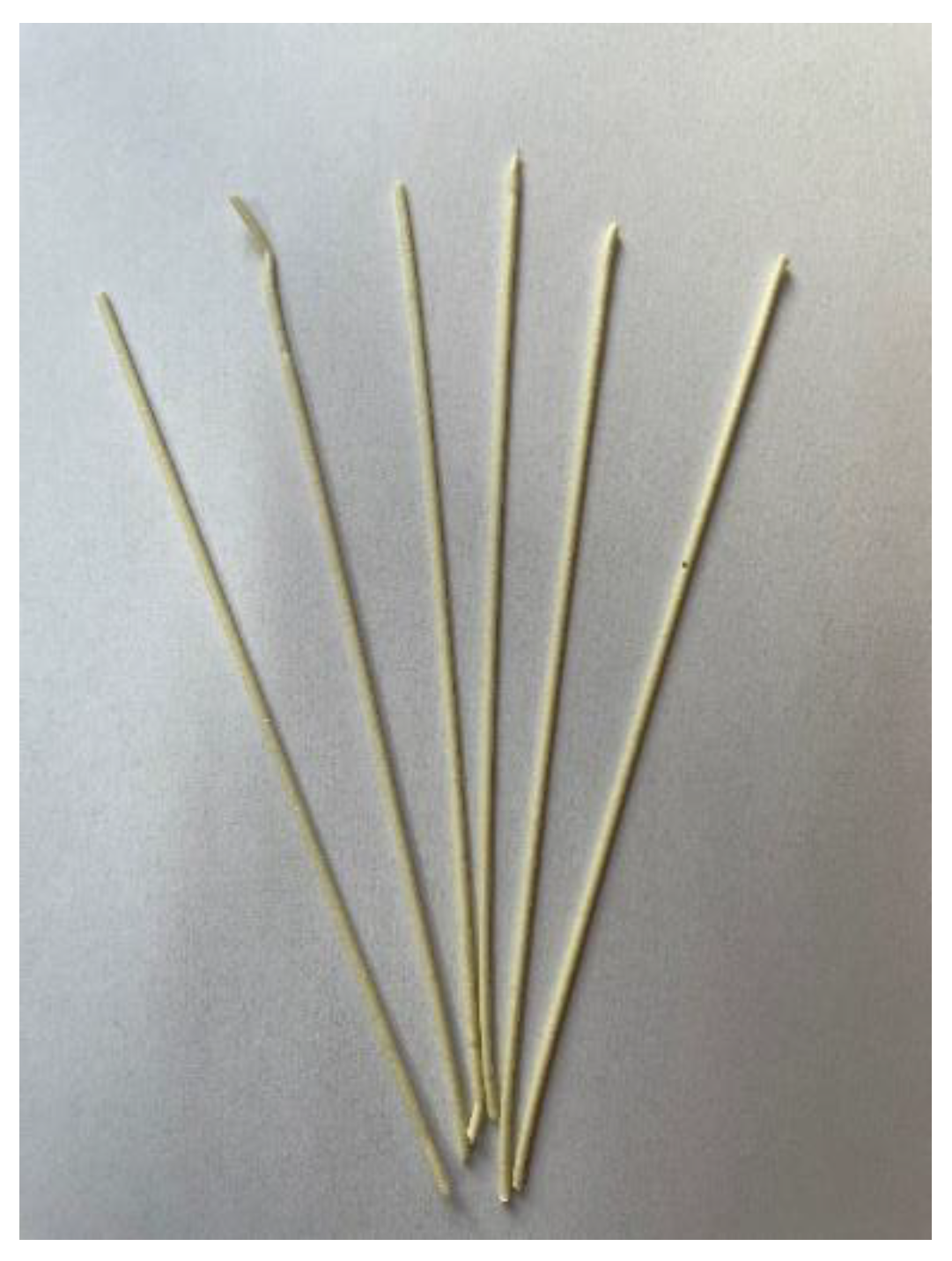
4 in the composite was 10 wt%. After granulation, the material was extruded at a temperature of 190 °C through a capillary nozzle with a diameter of 1.6 mm and aspect ratio L/D=12. The resulting printing filament had a diameter of 1.7 mm, see
Figure 2.
2.7. Nanofibers Prepared by DC and AC Electrospinning
Electrospinning is currently considered to be the simplest technology for producing fibers with precisely defined properties [
21], which uses a solution or melt and which is simultaneously based on and uses an electrostatic field during production. [
22,
23]. Fiber formation using a combination of electrostatic field and other forces is the goal of modern efforts to increase the range of electrospinning manufacturing options. Examples of this include the use of low frequencies [
24], high frequencies [
25] or air blowing [
26]. However, another study [
27] has shown that a static direct current (DC) high voltage source can be replaced by dynamic AC power, with significant productivity gains. The differences between the different approaches to the use of AC or DC electrospinning can be summarised as follows: The use of a dynamic AC voltage leads to a several-fold increase in productivity (using the same device) compared to DC voltage in the case of multiple fluid streams that are ejected from a continuously charged and discharged droplet – thus the AC being more permeable [
27,
28]. Operation without collector. The motion of the flying nanofibre plough produced by AC voltage electrospinning is not affected by the ground potential but by the electric field surrounding the spinneret. This means that it is not necessary to have a grounded collector. When producing fibers in a confined environment (e.g., pharmaceutical manufacturing), collection is more efficient if the problem of fiber stickiness that occurs with DCES on grounded surfaces (i.e., almost all surfaces except the charged spinneret) is eliminated [
29].Fibre production. Fiber materials are key ingredients for other high-value three-dimensional applications such as tissue engineering or composites. However, their fabrication using the commonly used DCES method is difficult due to the occurrence of repulsion between the flying fibers [
30]. In contrast, using AC electrospinning, twisted yarns can be easily produced without complex collection problems [
27,
31,
32].
Various factors affecting the process. In addition to the key factors that affect DCES (e.g. polymer concentration, electric field strength, etc.), there are other possibilities such as adjusting the frequency and shape of the AC voltage waveform. These changes could be used to optimize the ACES process, for example, in terms of productivity or morphology of the resulting fibers [
29].
A paper has been published [
33] where g-C
3N
4 was incorporated by electrospinning into PVDF fibers in order to prepare a membrane for use in the photocatalytic degradation of pollutants (the experiment was executed on Rhodaamine B) and subsequently another experiment has been published by essentially the same authors [
20], where C
3N
4 was doped into fibers with graphene oxide in a similar manner as described in this publication. Introduction of gC
3N
4 as a composite into PVB nanofibers by electrospinning was done at TUL.
- a)
DC electrospinning - NanospiderTM (Elmarco, CZ)
Sample 1.0, see Figure 33, control sample – polyvinyl butyral (PVB, B60H, Kuraray), 10 wt% PVB solution in ethanol. Electrospinning - NanospiderTM – electric voltage on spinning electrode +30 kV; electric voltage on collector -10 kV; electrode spacing 200 mm; diameter of the dosing device 0.7 mm; travel speed of the dosing device 1 sec/50 cm; relative humidity 40%; temperature 22°C; substrate material - spunbond-type non-woven fabric 30 g/m2 (PFNonwovens, CZ); substrate material removal rate 20 mm/min.
Sample 1.1, see Figure 34, - 10 wt% PVB in ethanol with the addition of 20 wt% g-C3N4 from dry matter of the polymer. The final theoretical concentration is 16.67 wt% gC3N4 from dry matter of the resulting fibers. The formation of the solution was in the following procedure: weighing a quantity of ethanol, adding g-C3N4 powder crushed into smaller particles in a mortar grinder, sonication by ultrasonic homogenizer 5x10 sec; adding PVB, mixing on a magnetic mixer for 8 hours. Electrospinning - NanospiderTM – electric voltage on spinning electrode +30 kV; electric voltage on collector -10 kV; electrode spacing 200 mm; diameter of the dosing device 0.7 mm; travel speed of the dosing device 1 sec/50 cm; relative humidity 40%; temperature 22°C; substrate material - spunbond-type non-woven fabric 30 gm -2 (PFNonwovens, CZ), see Figure 35; substrate material removal rate 20 mm/min.
- b)
AC electrospinning – rod electrode (TUL)
Sample 2.1, see Figure 36 – AC electrospinning was carried out on equipment developed by the TUL FP and FS team. The spinning process took place under the following conditions: Effective voltage Uef 35 kV; sine wave signal; frequency 50 Hz; distance of the black paper (electrically inactive collector) from the rod spinning electrode 350 mm; relative humidity 40%; temperature 22°C.
Figure 1.
Initial precursors of the synthesis process of g-C3N4, structures of nanosheets.
Figure 1.
Initial precursors of the synthesis process of g-C3N4, structures of nanosheets.
Figure 2.
PP-gC3N4 filament samples.
Figure 2.
PP-gC3N4 filament samples.
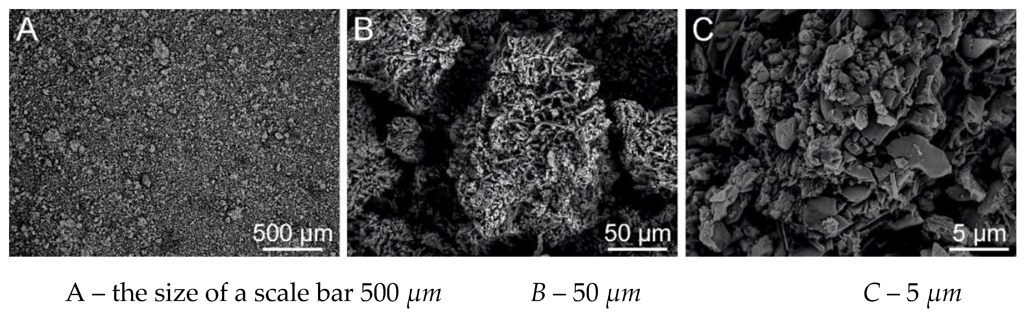
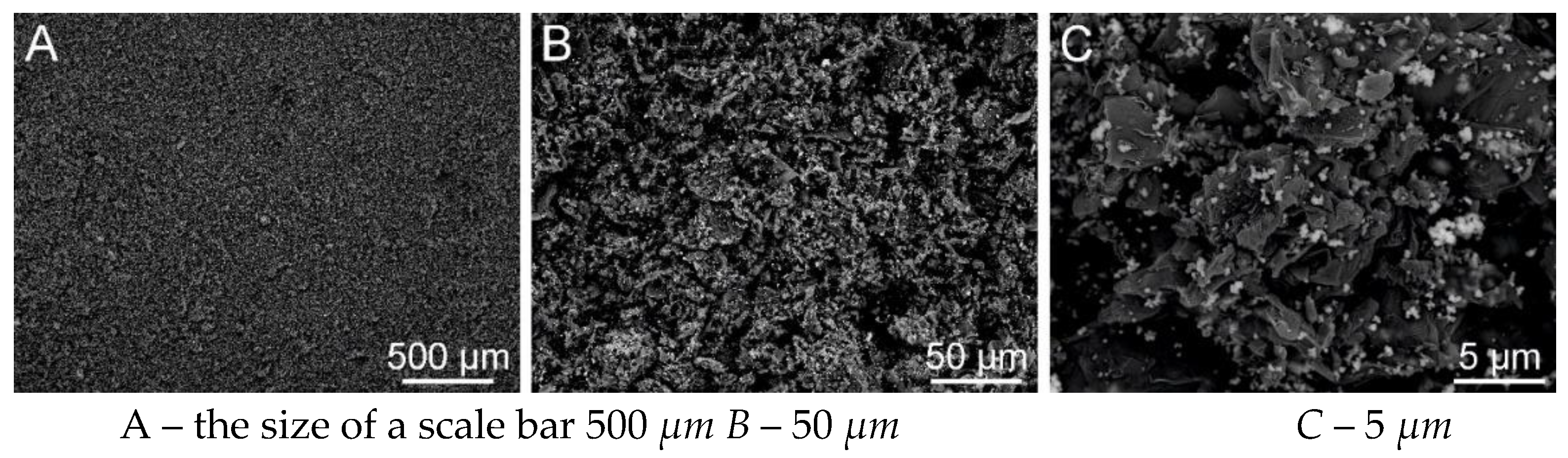
Figure 9.
SEM micrographs of g-C3N4, SEM: SE+BSE.
Figure 9.
SEM micrographs of g-C3N4, SEM: SE+BSE.
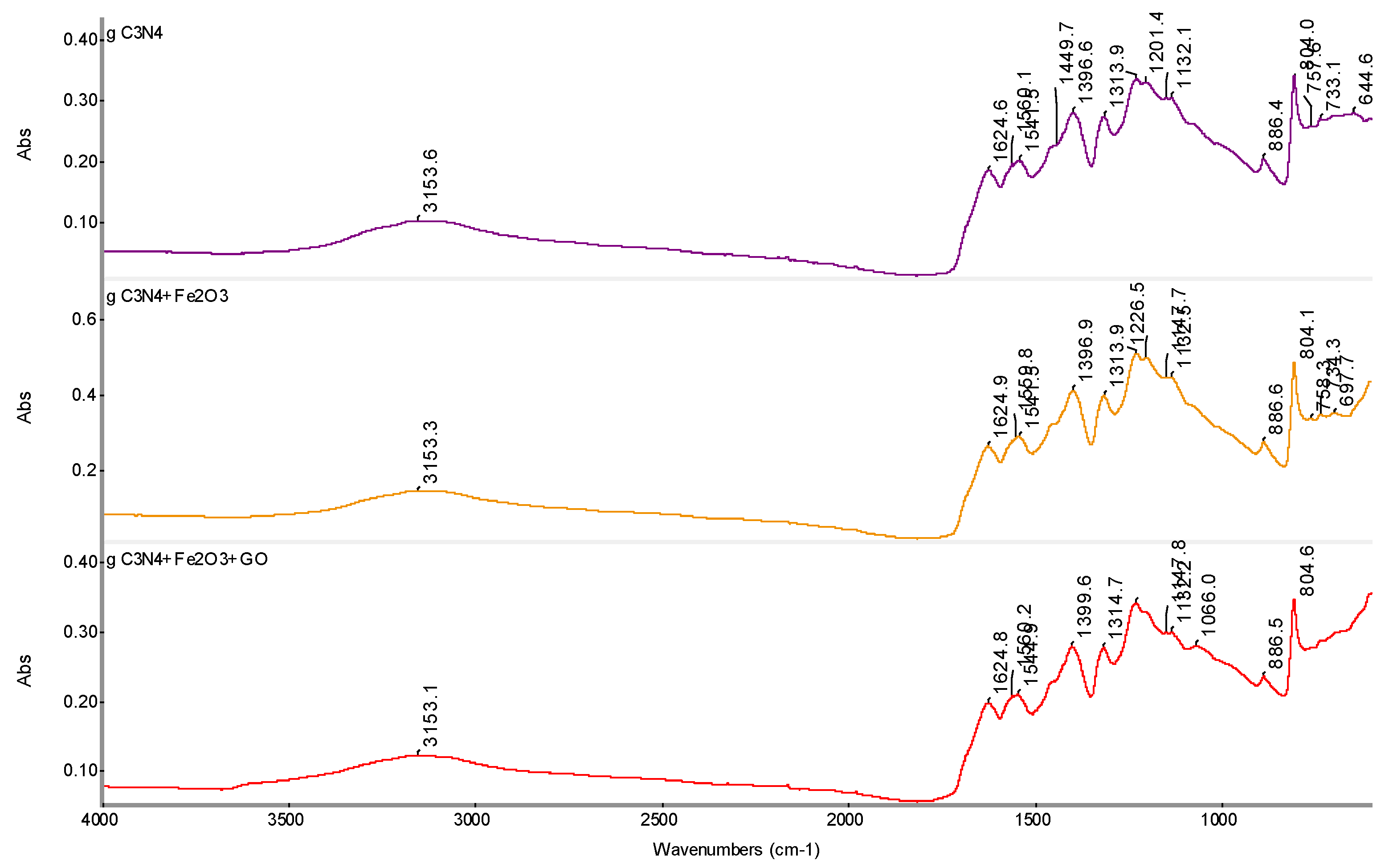
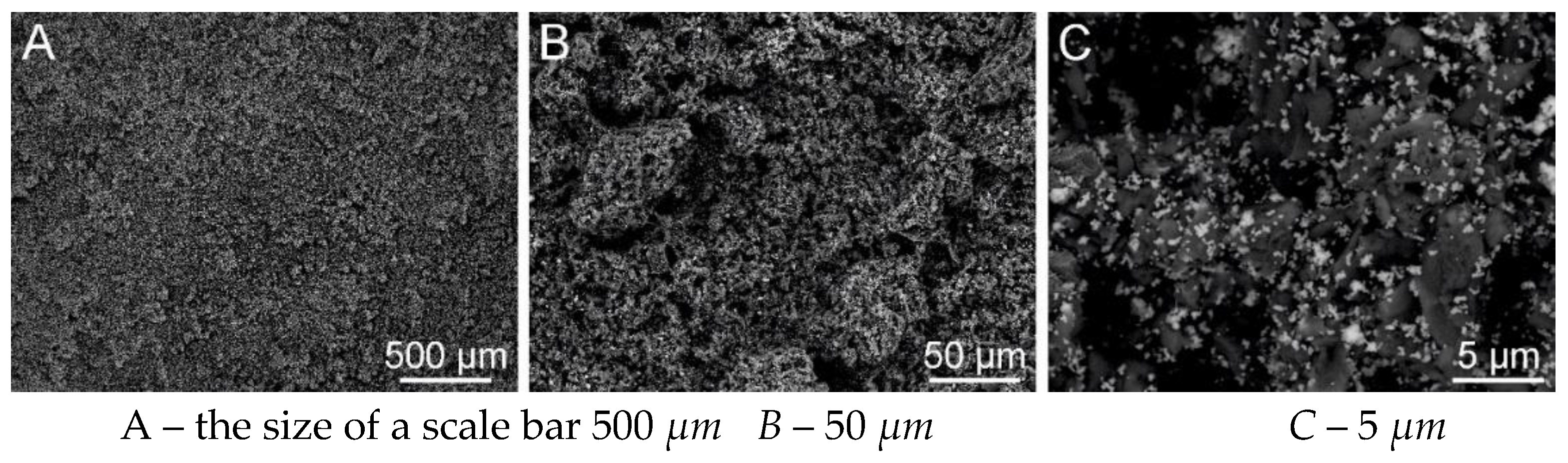
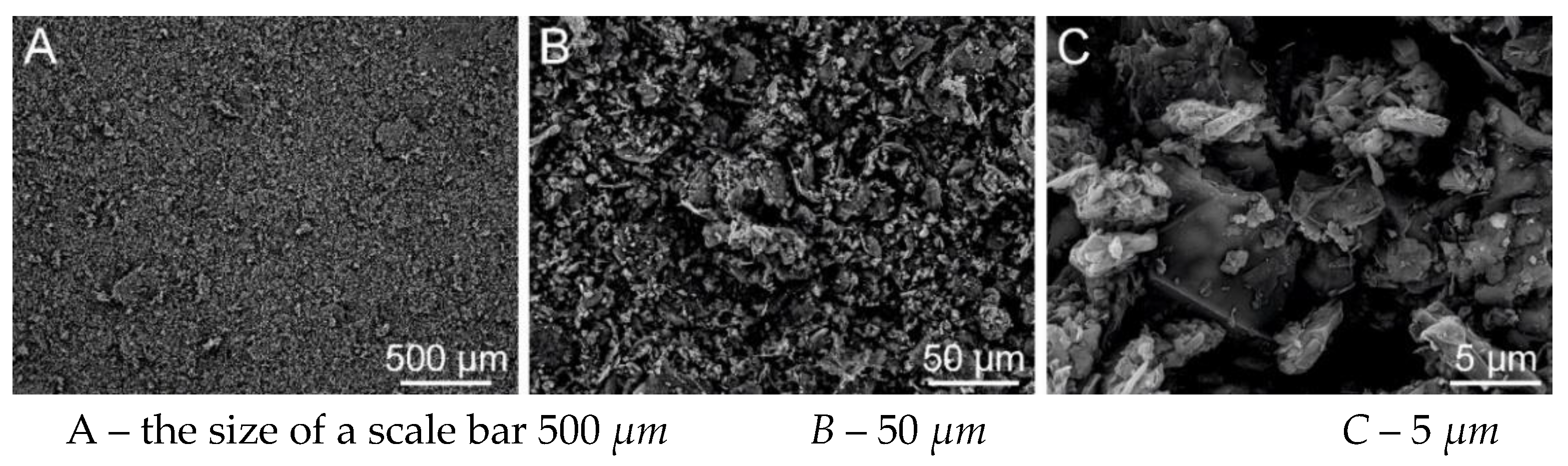
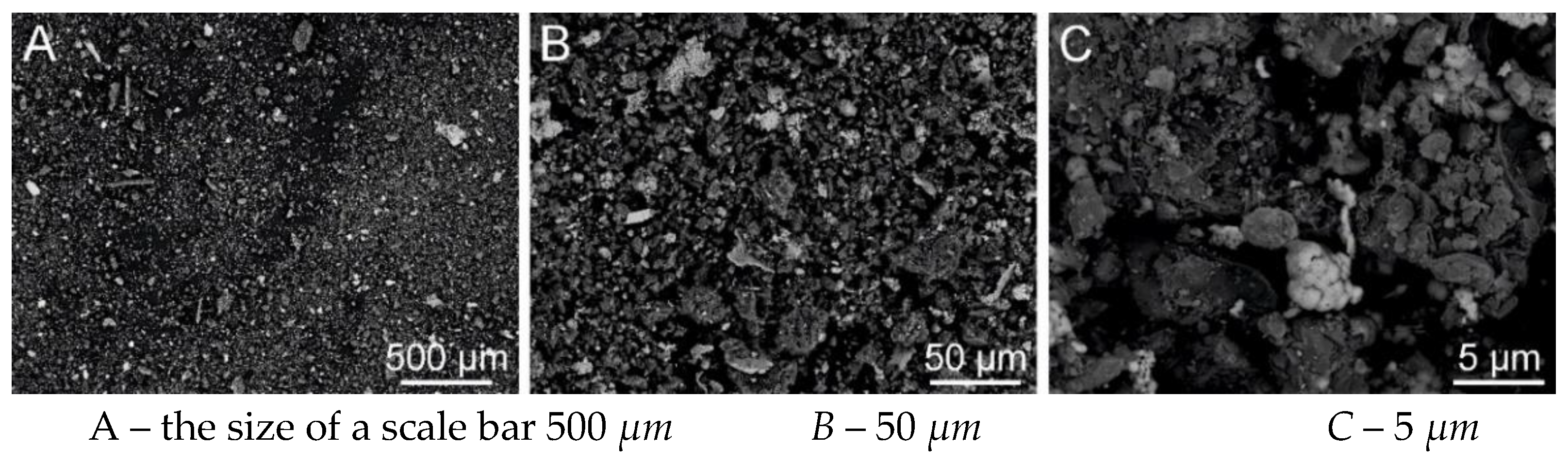
Figure 10.
SEM analysis of g-C3N4 + Fe2O3, SEM: SE+BSE (Tescan Vega 4).
Figure 10.
SEM analysis of g-C3N4 + Fe2O3, SEM: SE+BSE (Tescan Vega 4).
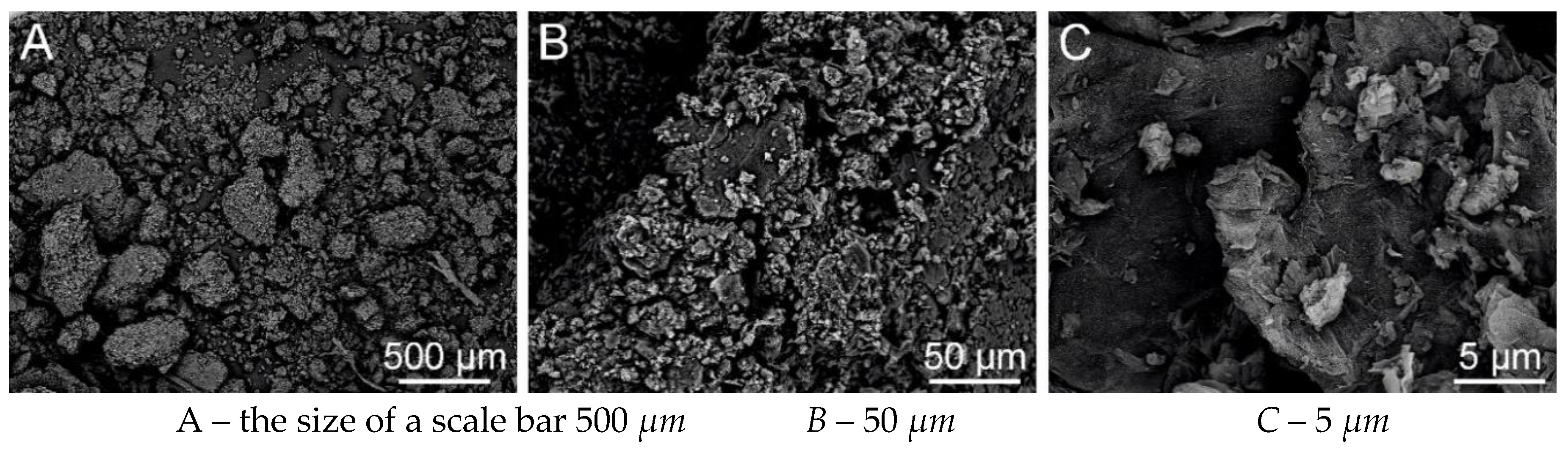
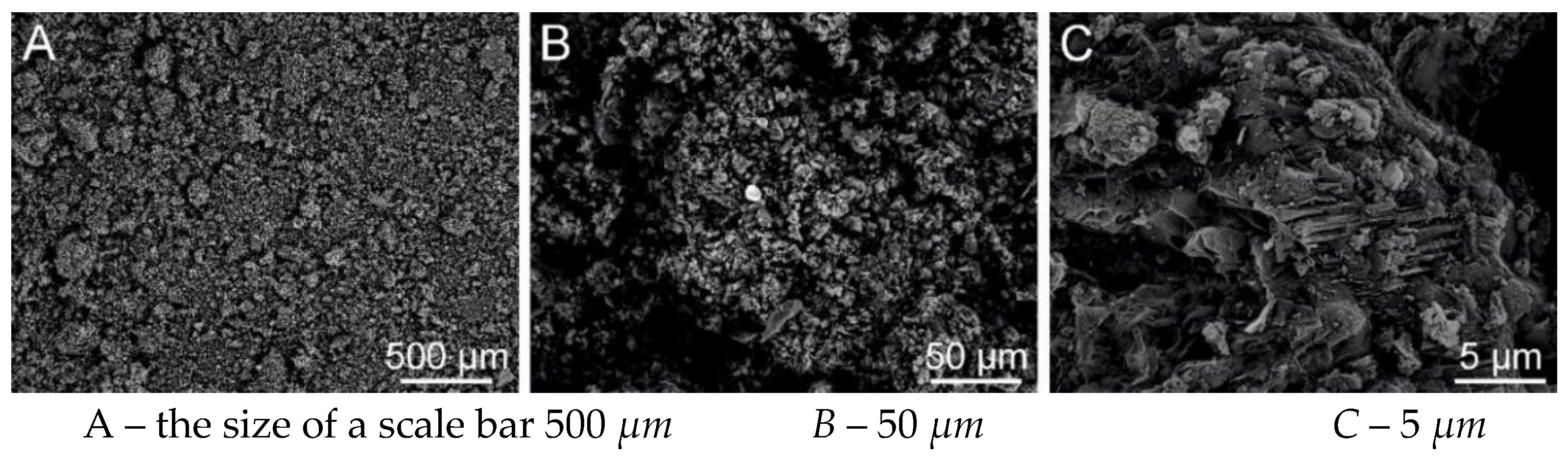
Figure 11.
SEM analysis of g-C3N4 + Fe2O3 + GO, SEM: SE+BSE(Tescan Vega 4).
Figure 11.
SEM analysis of g-C3N4 + Fe2O3 + GO, SEM: SE+BSE(Tescan Vega 4).
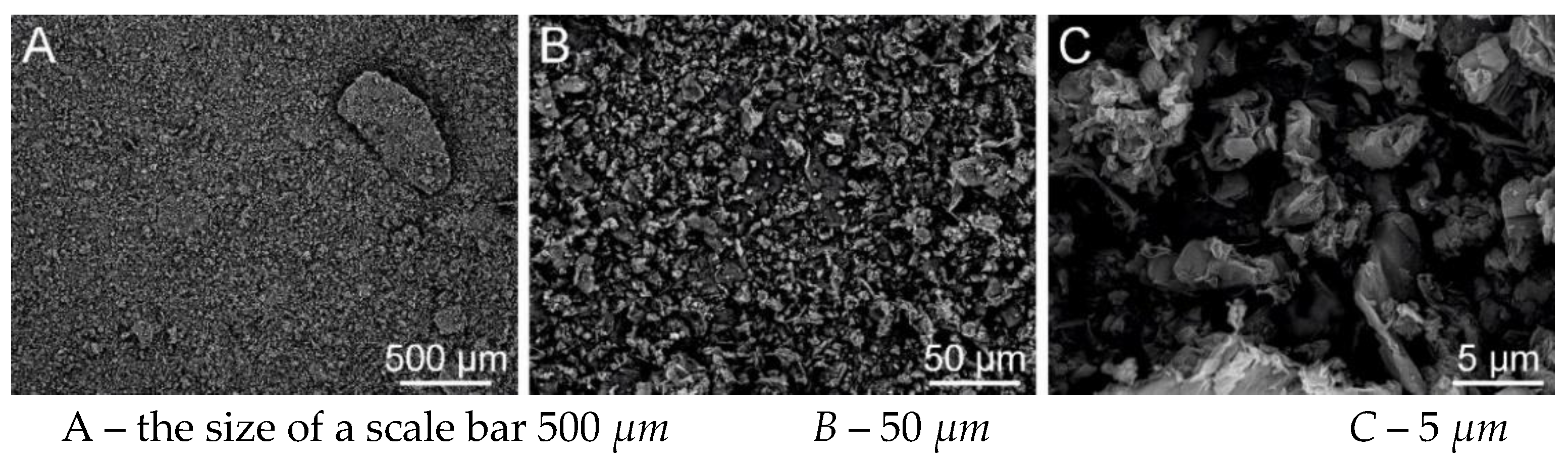
Figure 12.
SEM analysis of g-C3N4 + rGO, SEM: SE+BSE (Tescan Vega 4).
Figure 12.
SEM analysis of g-C3N4 + rGO, SEM: SE+BSE (Tescan Vega 4).
Figure 13.
SEM analysis of g-C3N4 + GO, SEM: SE+BSE (Tescan Vega 4).
Figure 13.
SEM analysis of g-C3N4 + GO, SEM: SE+BSE (Tescan Vega 4).
Figure 14.
SEM analysis of g-C3N4 + GO + 30% H2O2, SEM: SE+BSE (Tescan Vega 4).
Figure 14.
SEM analysis of g-C3N4 + GO + 30% H2O2, SEM: SE+BSE (Tescan Vega 4).
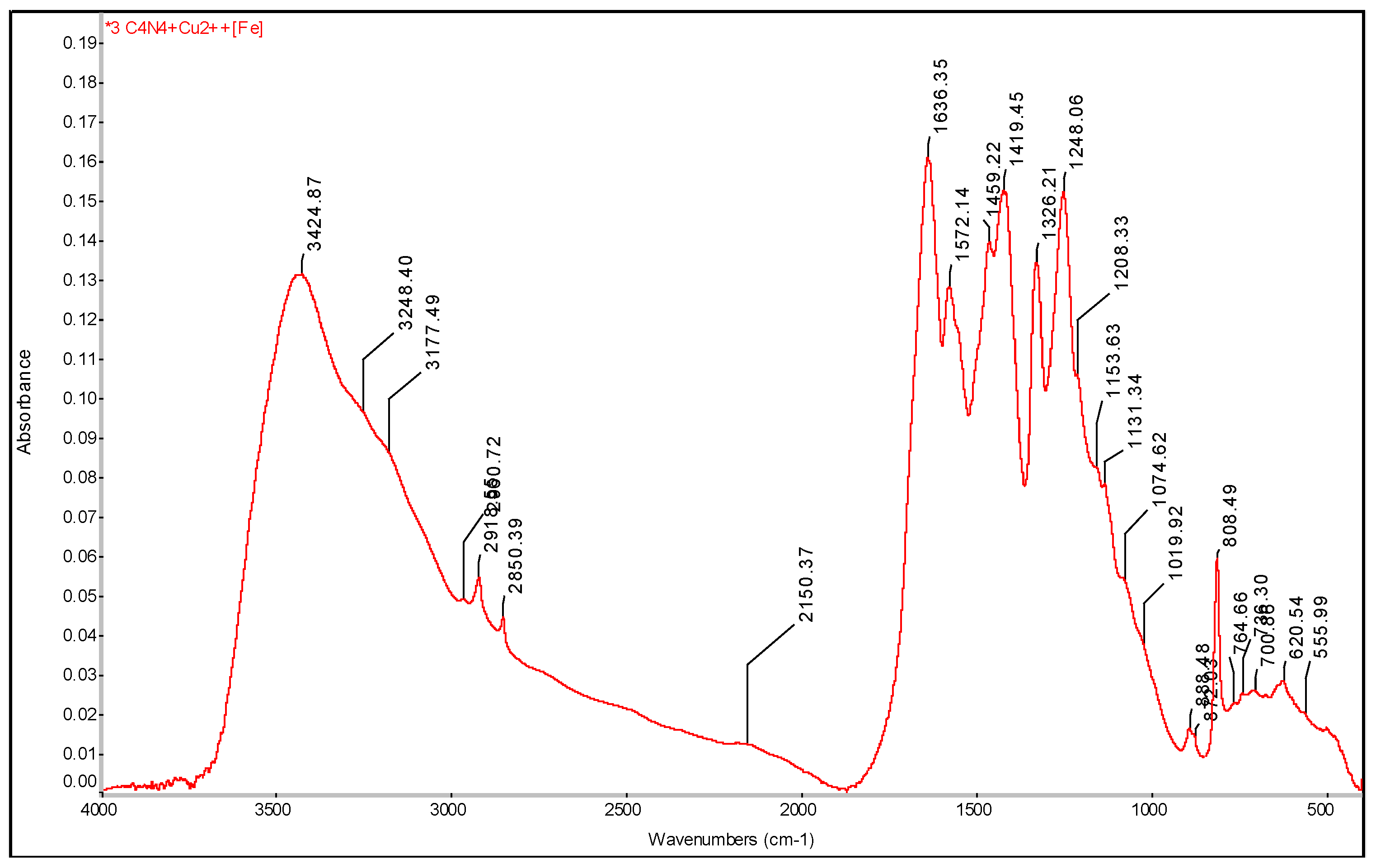
Figure 15.
SEM analysis of g-C3N4 + Cu2+[Fe], SEM: SE+BSE (Tescan Vega 4) .
Figure 15.
SEM analysis of g-C3N4 + Cu2+[Fe], SEM: SE+BSE (Tescan Vega 4) .
Figure 16.
SEM analysis of melamine 511°C - GO, SEM: SE+BSE (Tescan Vega 4).
Figure 16.
SEM analysis of melamine 511°C - GO, SEM: SE+BSE (Tescan Vega 4).
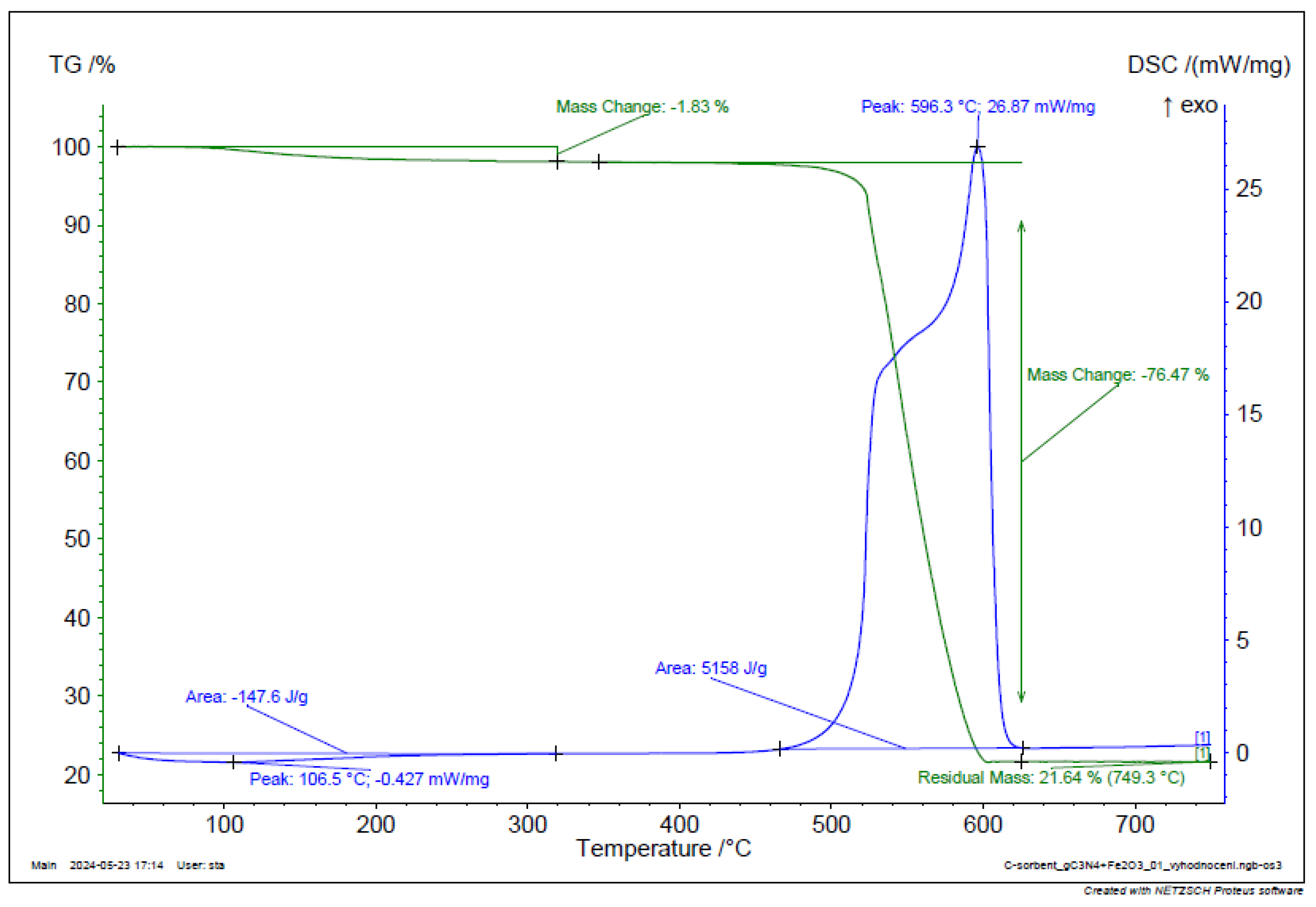
Figure 17.
TGA and DSC analysis of g-C3N4 + Fe2O3.
Figure 17.
TGA and DSC analysis of g-C3N4 + Fe2O3.
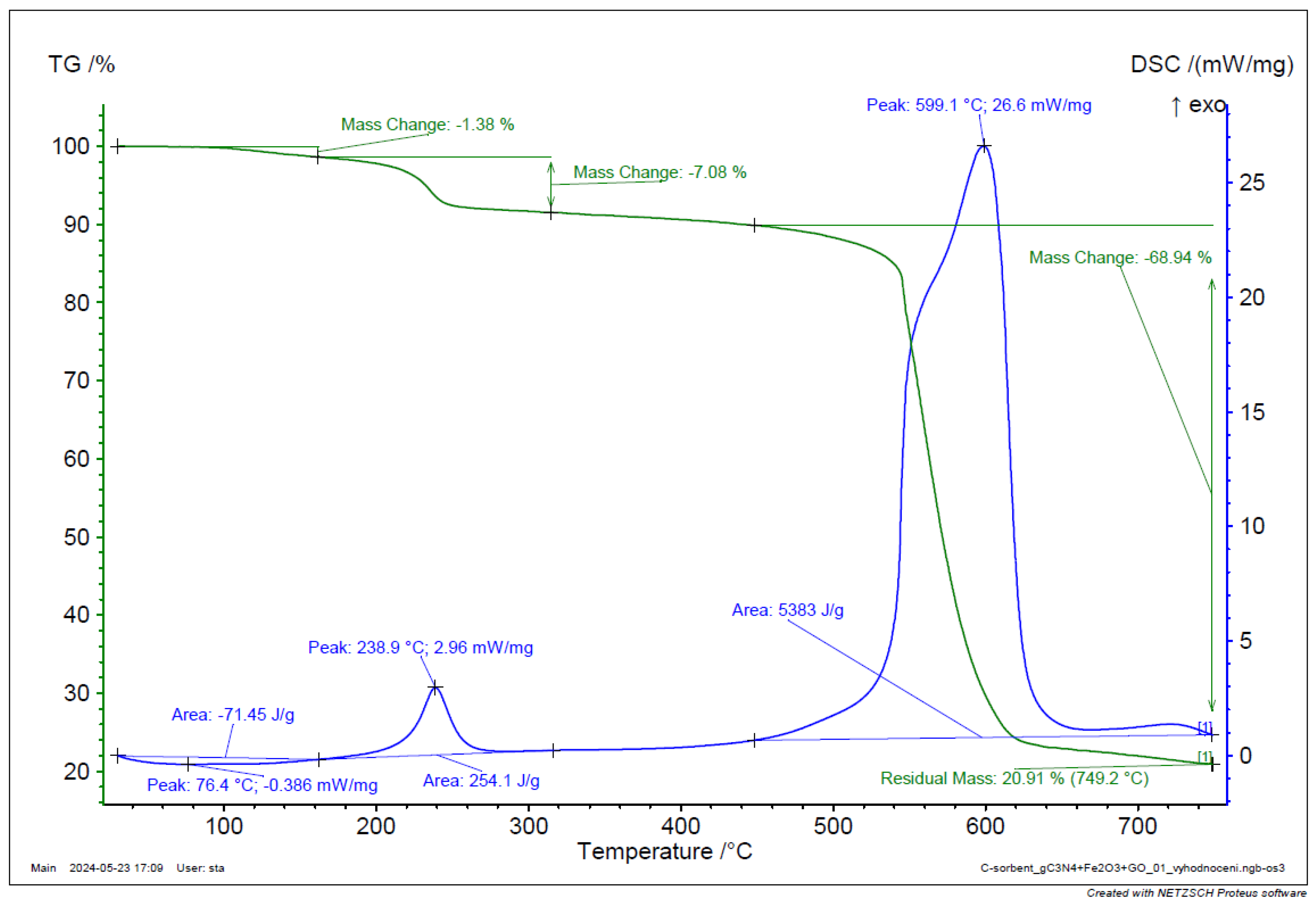
Figure 18.
TGA and DSC analysis of g-C3N4 + Fe2O3 + GO.
Figure 18.
TGA and DSC analysis of g-C3N4 + Fe2O3 + GO.
Figure 19.
TGA and DSC analysis of g-C3N4.
Figure 19.
TGA and DSC analysis of g-C3N4.
Figure 20.
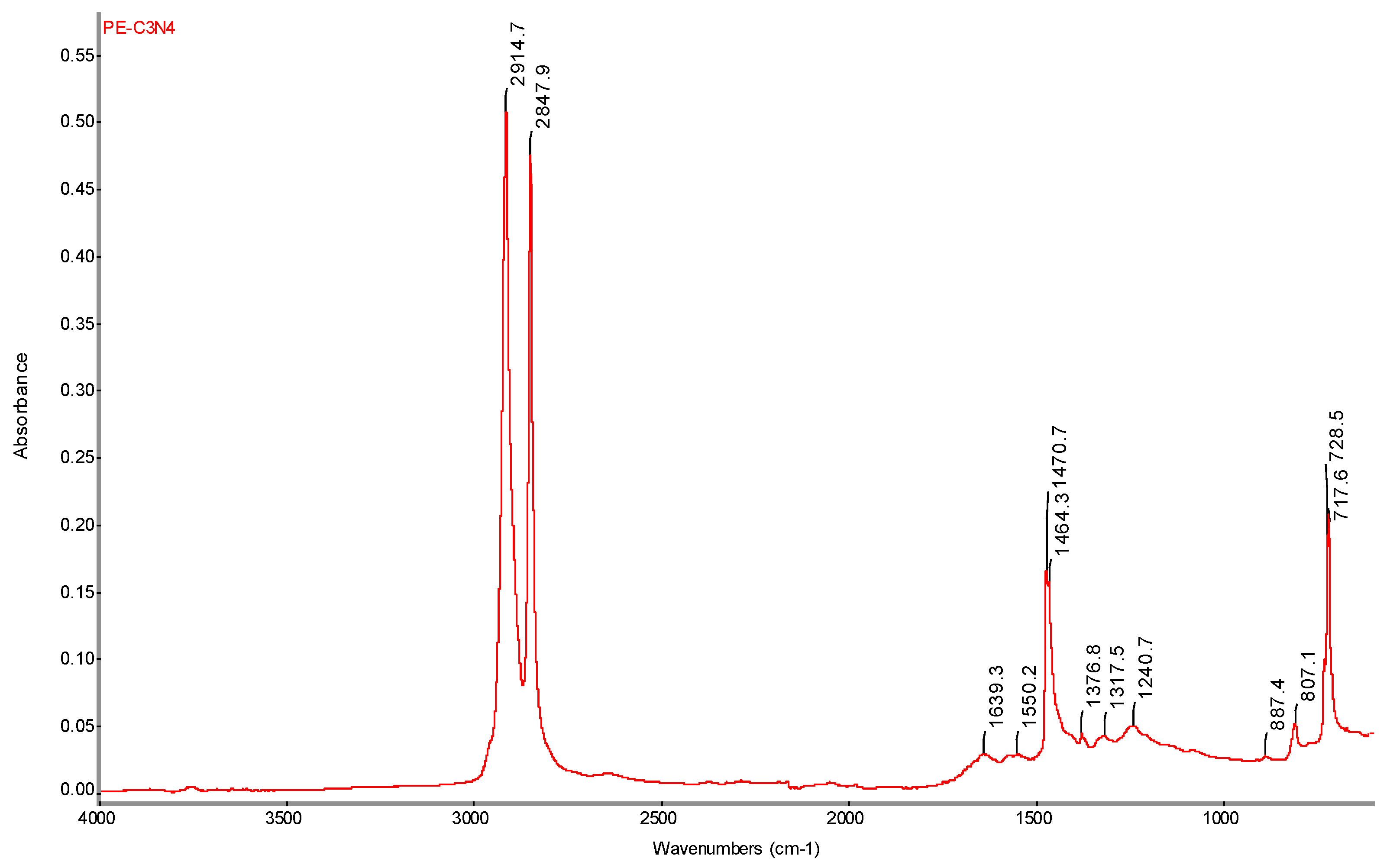
FTIR spectrum of PE-C3N4 with determination of characteristic bands.
Figure 20.
FTIR spectrum of PE-C3N4 with determination of characteristic bands.
Figure 21.
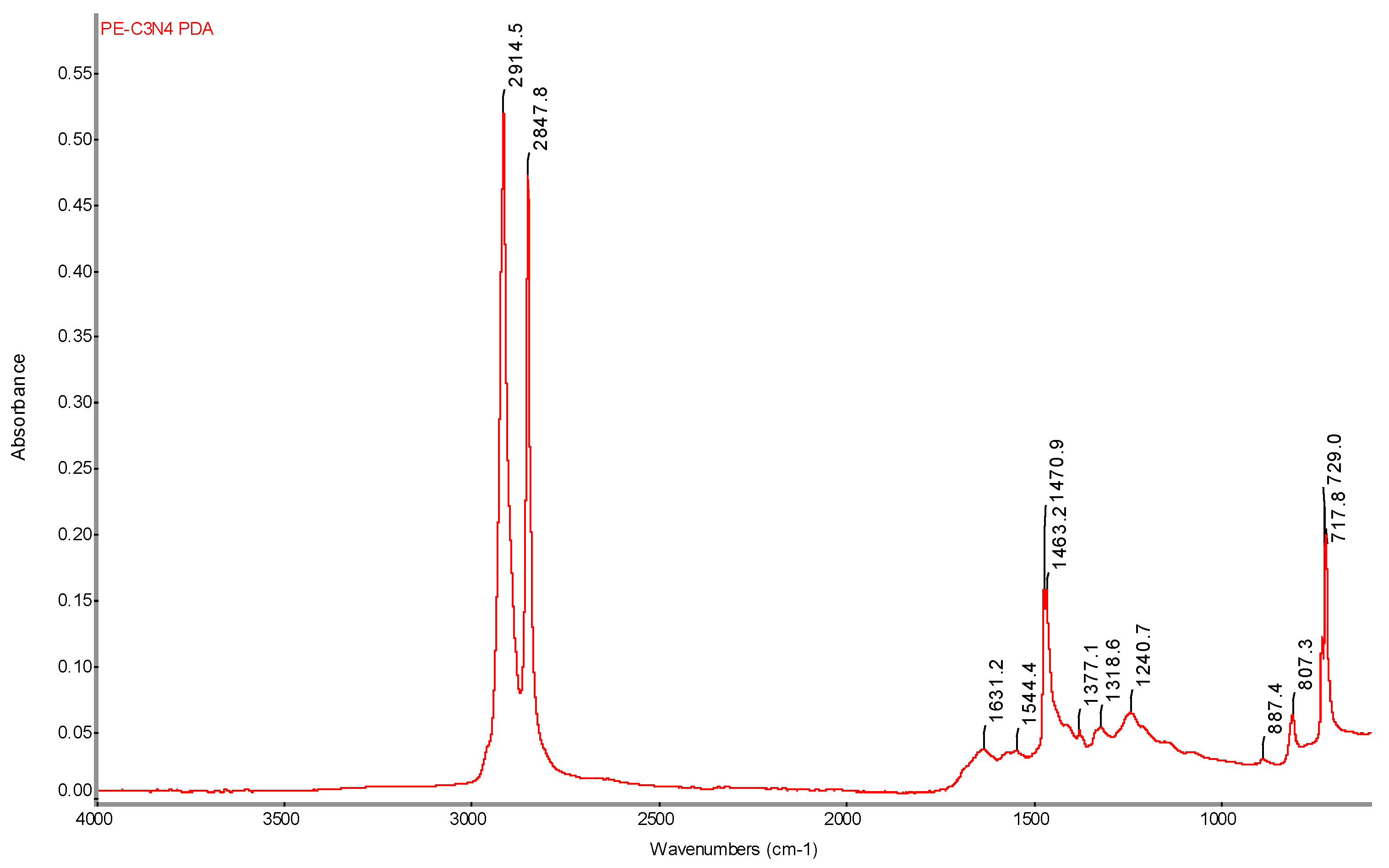
FTIR spectrum of PE-C3N4 PDA film with determination of characteristic bands.
Figure 21.
FTIR spectrum of PE-C3N4 PDA film with determination of characteristic bands.
Figure 22.
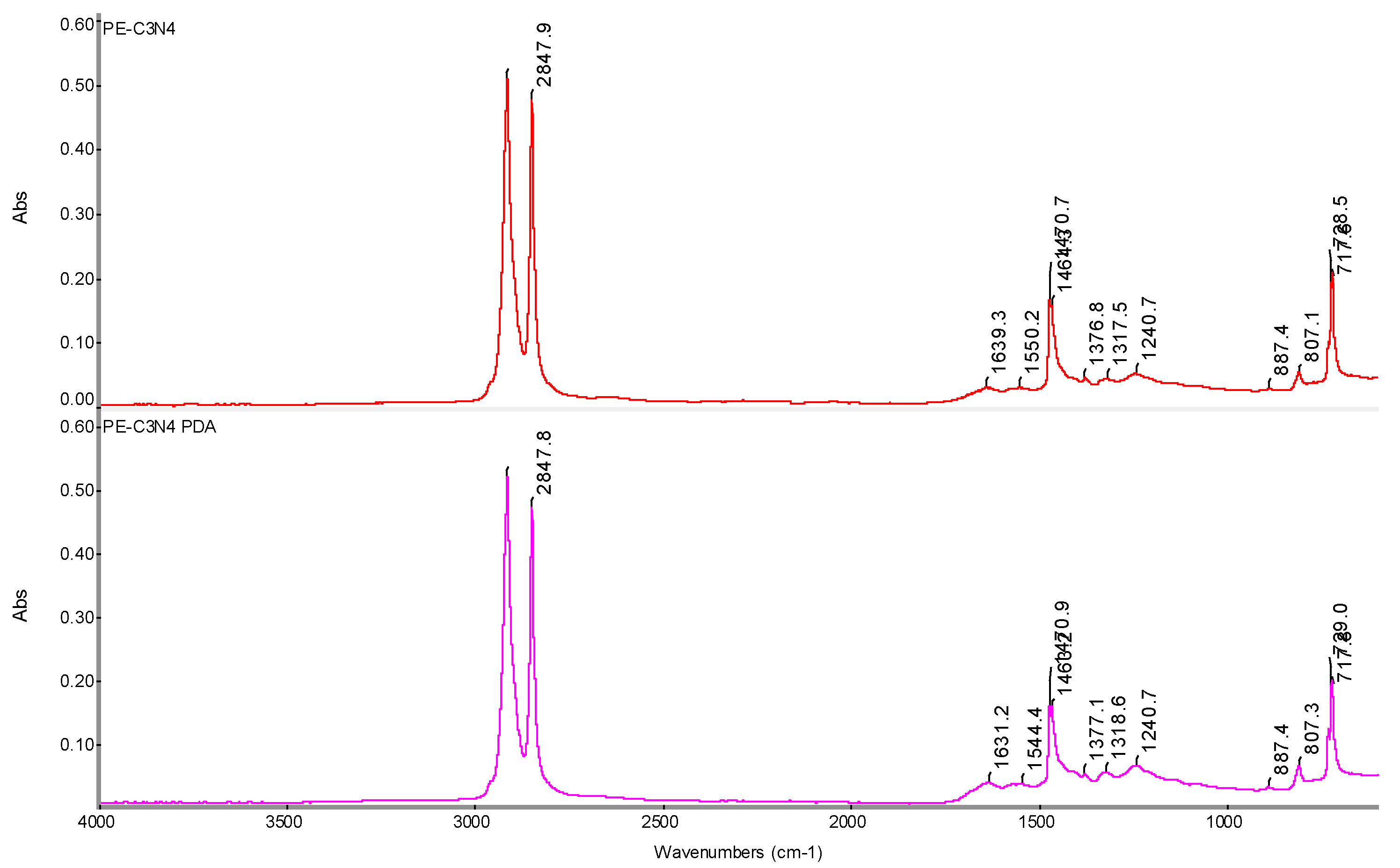
FTIR spectrum of PE-C3N4 and PE-C3N4 PDA films with determination of characteristic bands.
Figure 22.
FTIR spectrum of PE-C3N4 and PE-C3N4 PDA films with determination of characteristic bands.
Figure 23.
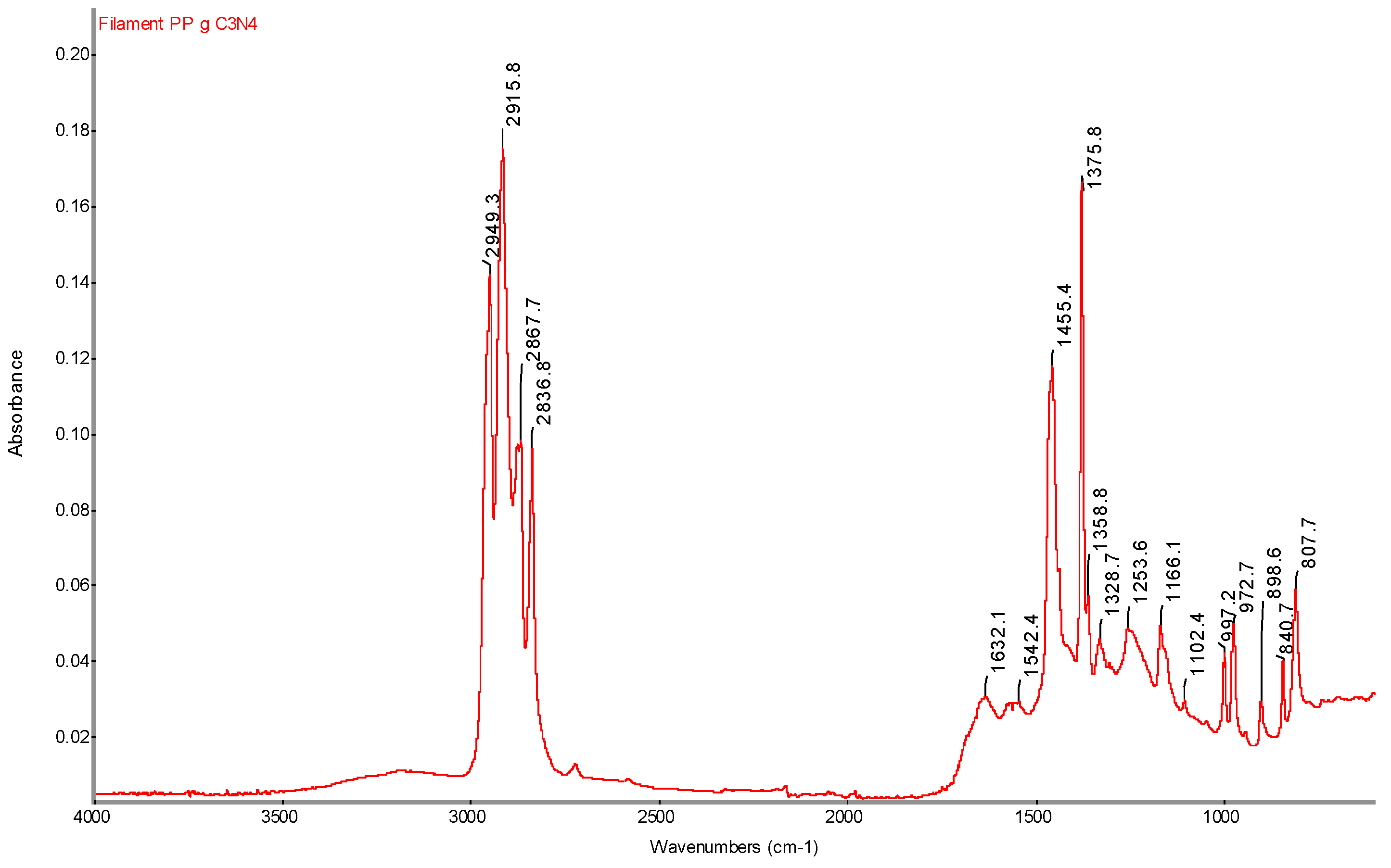
Infrared spectrum of PP g C3N4 filament sample with determination of characteristic bands.
Figure 23.
Infrared spectrum of PP g C3N4 filament sample with determination of characteristic bands.
Figure 24.
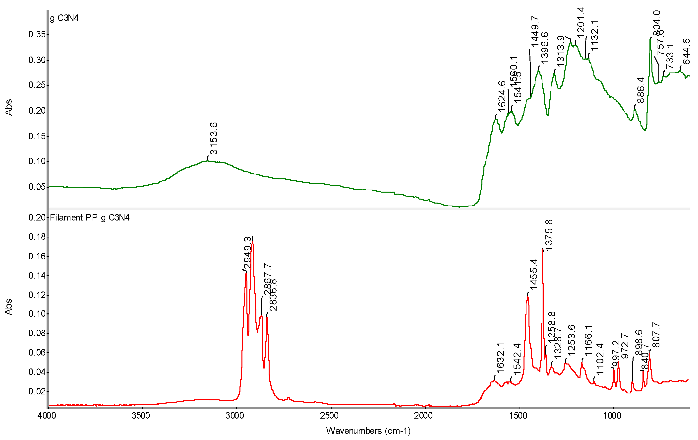
Comparison of FTIR spectra of initial gC3N4 and PP gC3N4 filament samples with determination of characteristic bands.
Figure 24.
Comparison of FTIR spectra of initial gC3N4 and PP gC3N4 filament samples with determination of characteristic bands.
Figure 25.
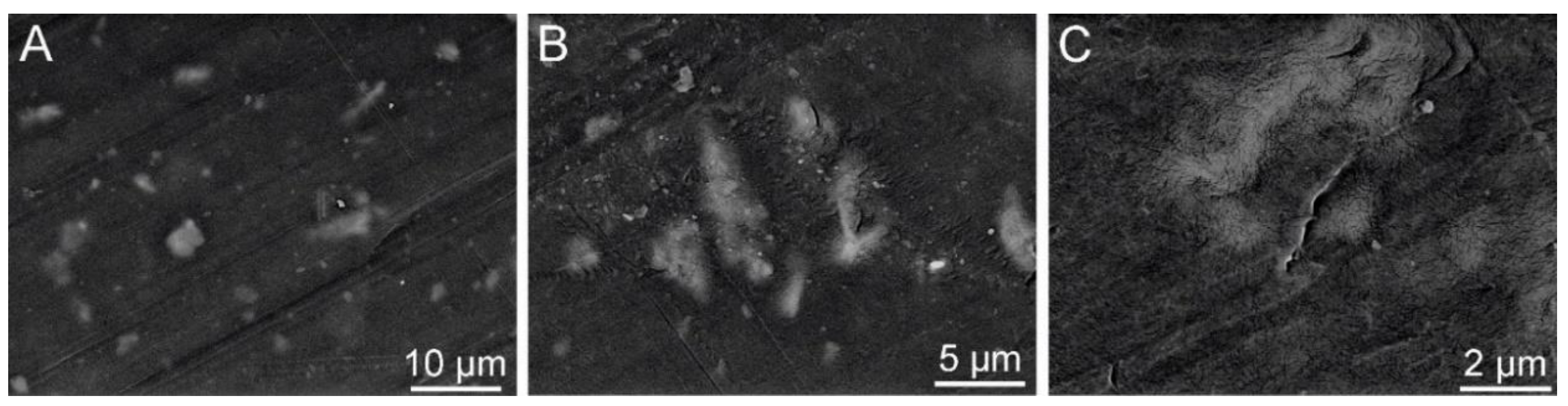
LDPE+g-C3N4 : SEM: SE+BSE A – the size of a scale bar 10 μm; B – 5 μm;C – 2 μm (Tesca Vegan 4).
Figure 25.
LDPE+g-C3N4 : SEM: SE+BSE A – the size of a scale bar 10 μm; B – 5 μm;C – 2 μm (Tesca Vegan 4).
Figure 26.
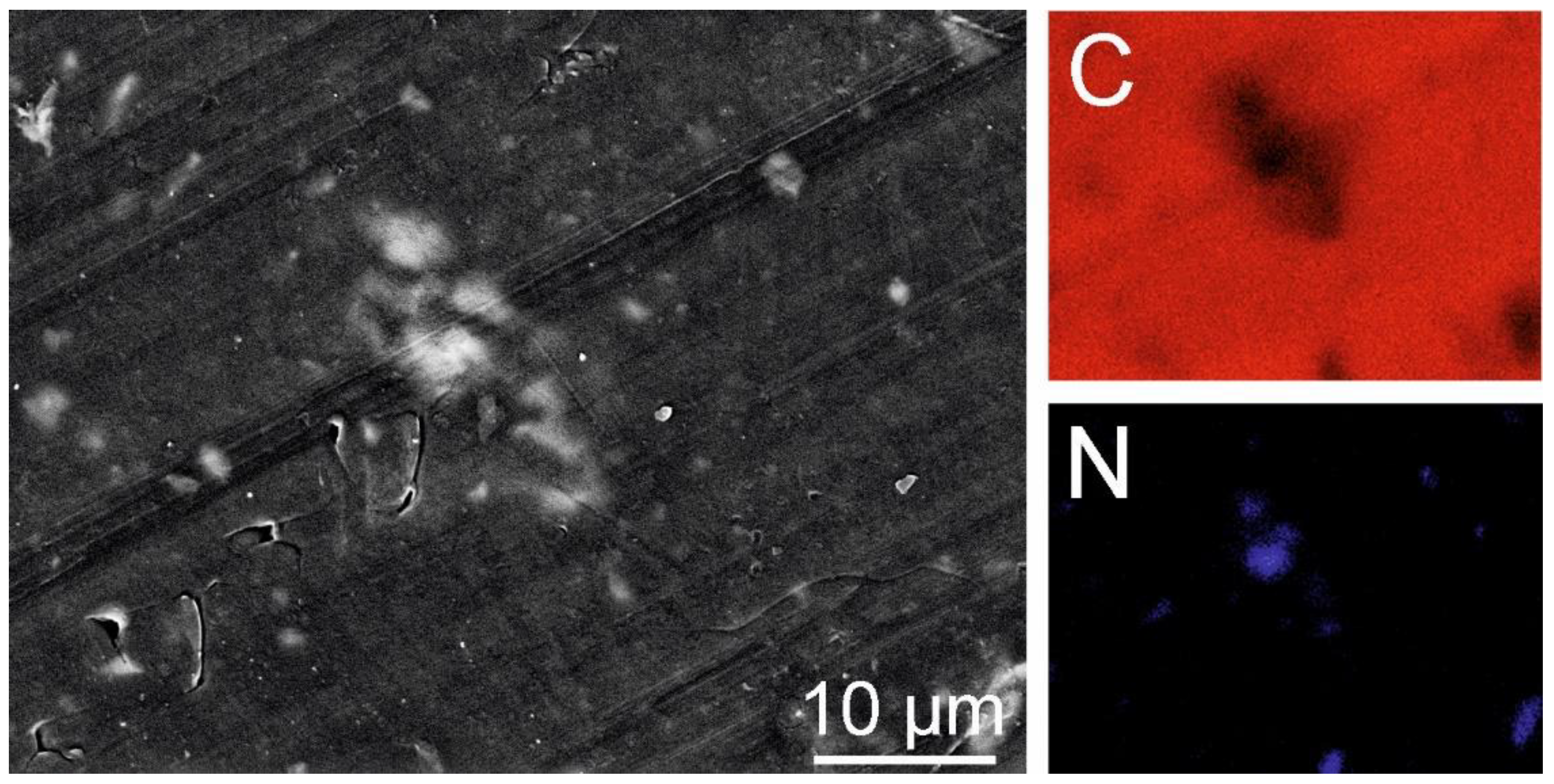
LDPE+C3N4 – EDS Mapping of C and N (Tesca Vegan 4).
Figure 26.
LDPE+C3N4 – EDS Mapping of C and N (Tesca Vegan 4).
Figure 27.
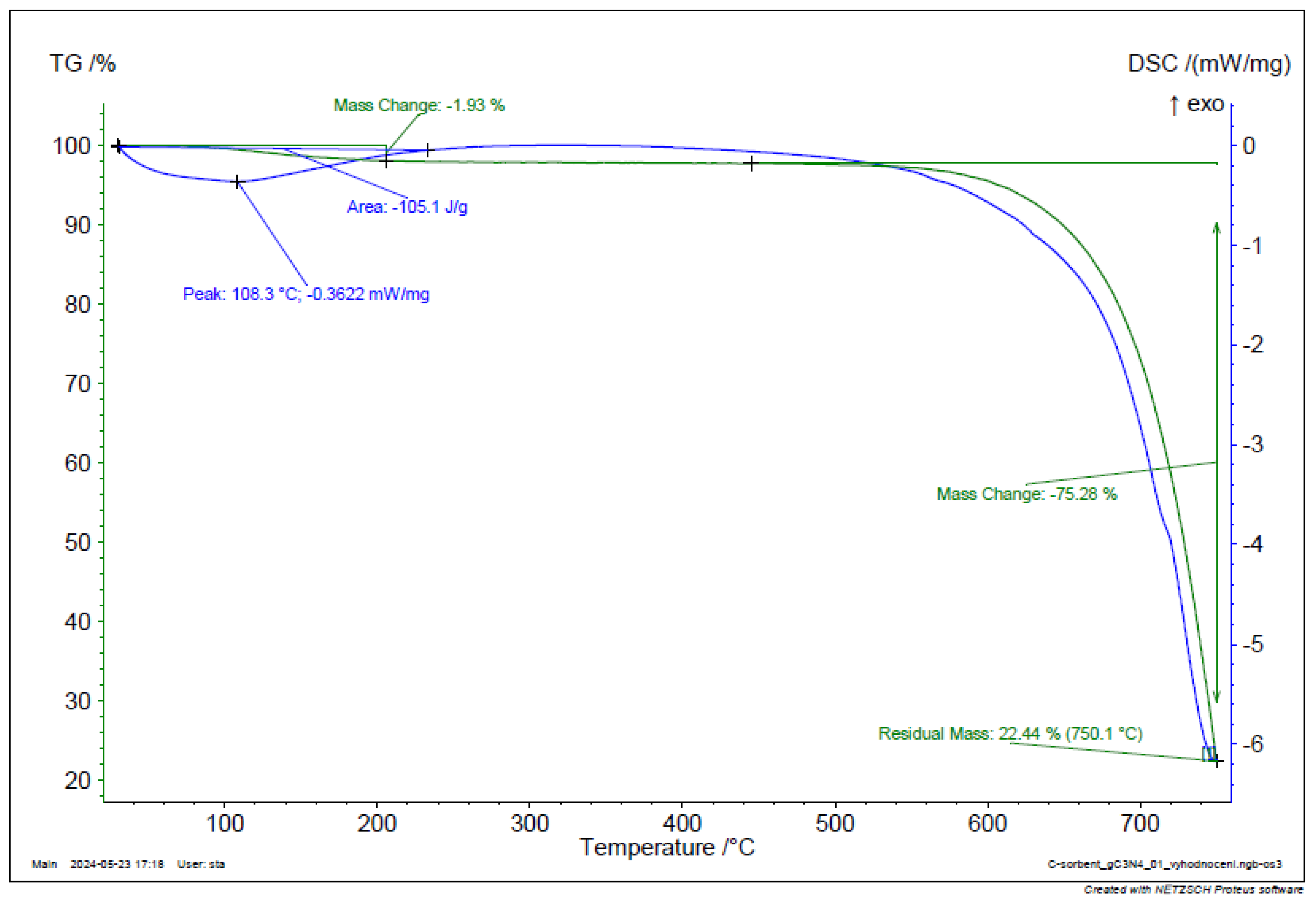
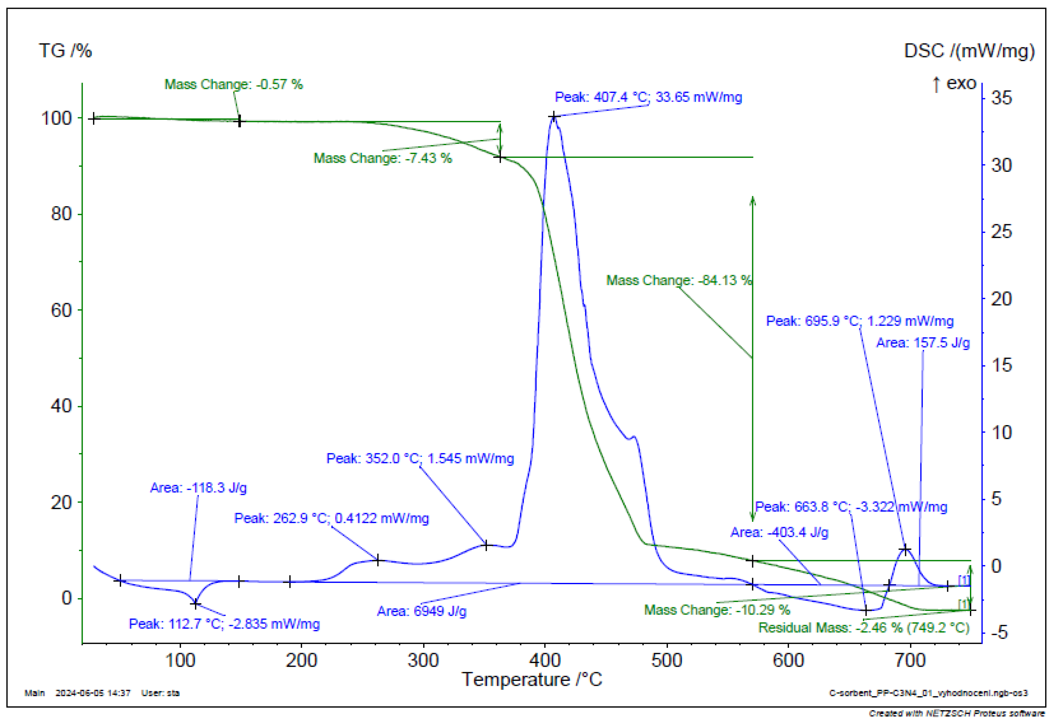
TGA and DSC analysis of g-C3N4-PE composite.
Figure 27.
TGA and DSC analysis of g-C3N4-PE composite.
Figure 28.
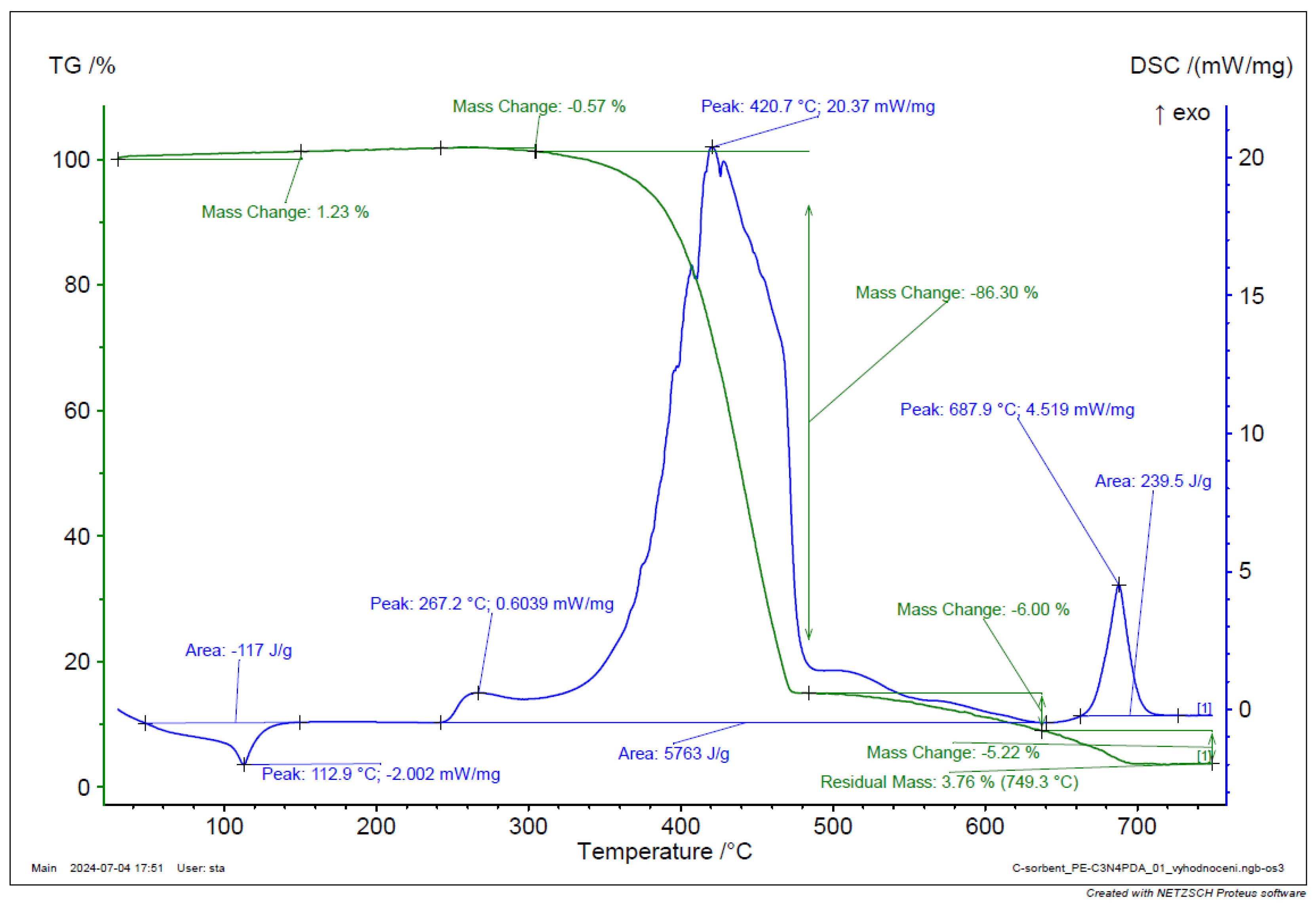
TGA and DSC analysis of g-C3N4-PDA-PE composite.
Figure 28.
TGA and DSC analysis of g-C3N4-PDA-PE composite.
Figure 29.
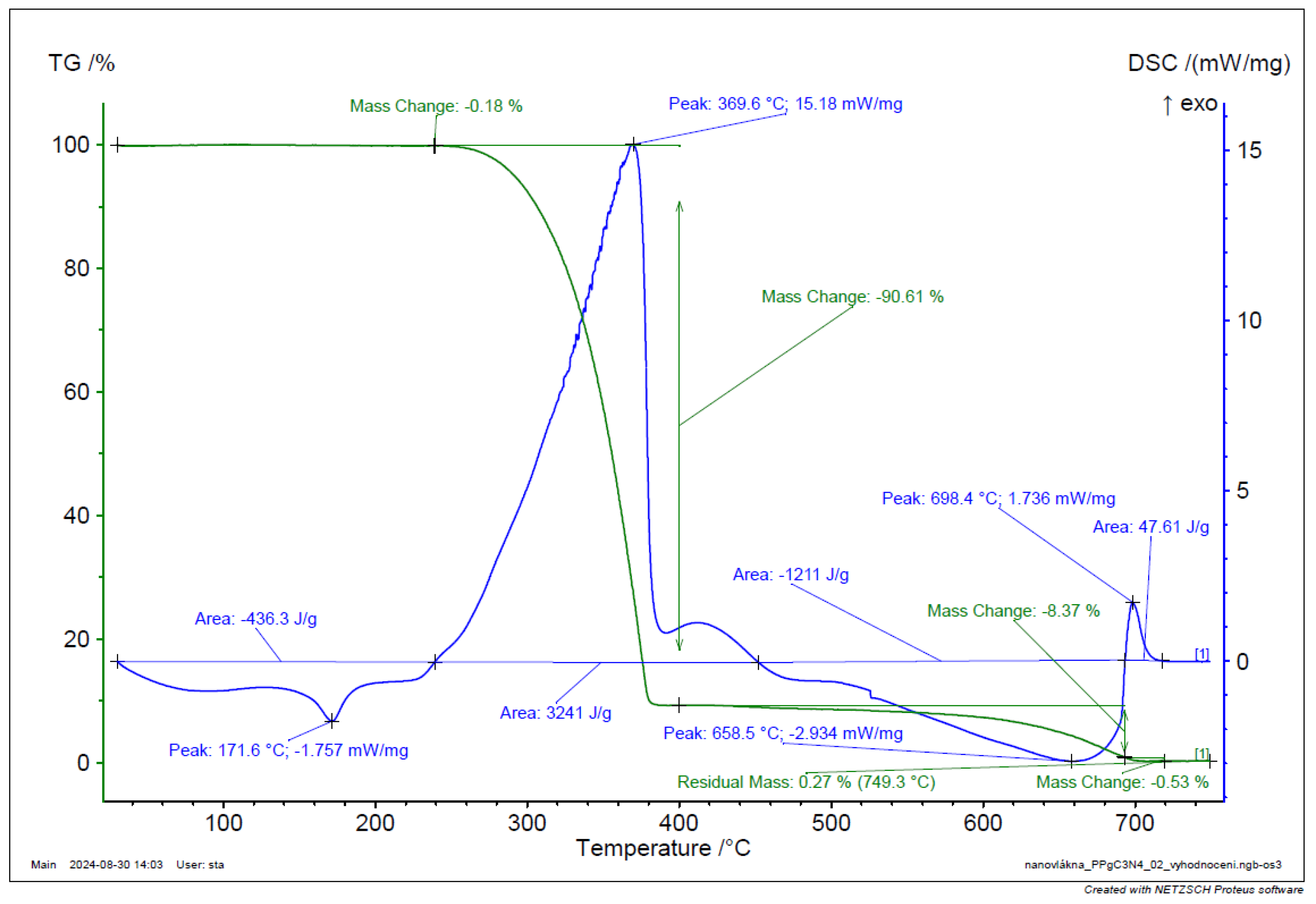
TGA and DSC analysis of PP-gC3N4 filament.
Figure 29.
TGA and DSC analysis of PP-gC3N4 filament.
Figure 30.
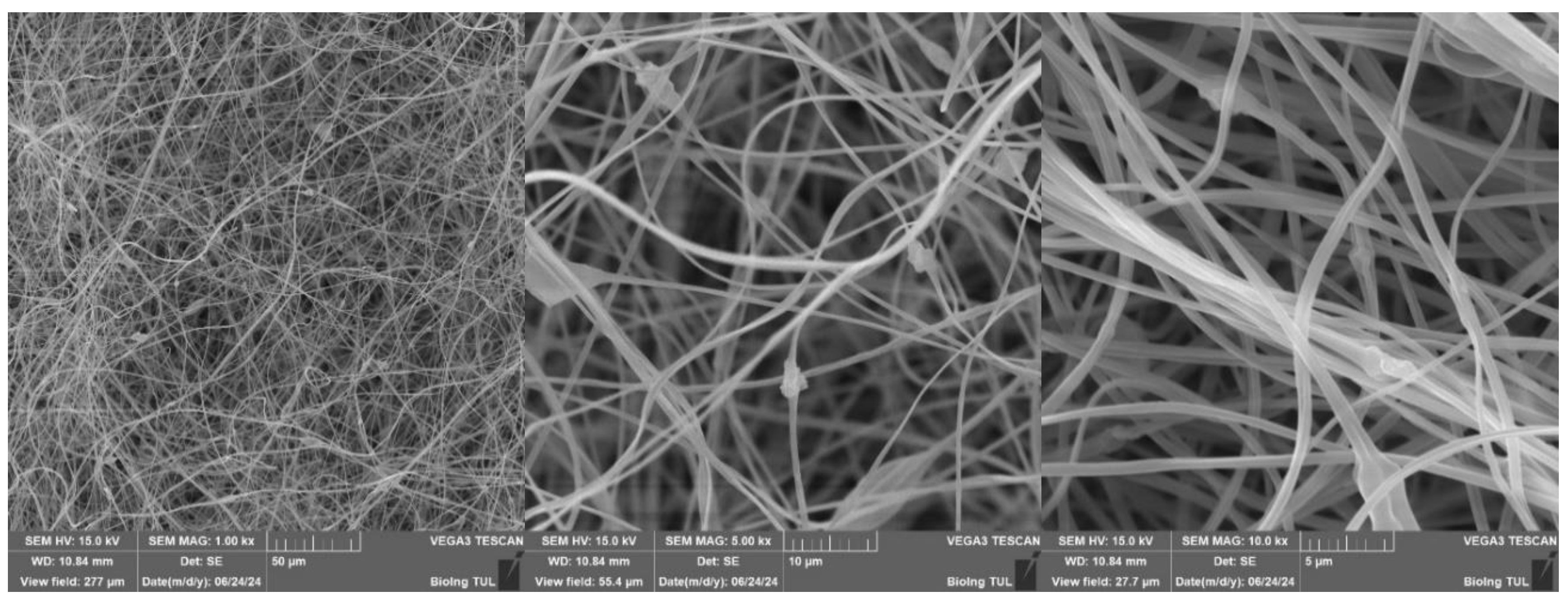
SEM analysis of PVB EL-DC nanofibers A – the size of a scale bar 50 μm; B – 10 μm; C - 5 μm (Tescan Vega 3 (TUL)).
Figure 30.
SEM analysis of PVB EL-DC nanofibers A – the size of a scale bar 50 μm; B – 10 μm; C - 5 μm (Tescan Vega 3 (TUL)).
Figure 31.
SEM analysis of PVB nanofiber with g-C3N4 EL-DC (A – the size of a scale bar 500 μm; B – 50 μm; C –5 μm) (Tesca Vegan 3 (TUL)).
Figure 31.
SEM analysis of PVB nanofiber with g-C3N4 EL-DC (A – the size of a scale bar 500 μm; B – 50 μm; C –5 μm) (Tesca Vegan 3 (TUL)).
Figure 32.
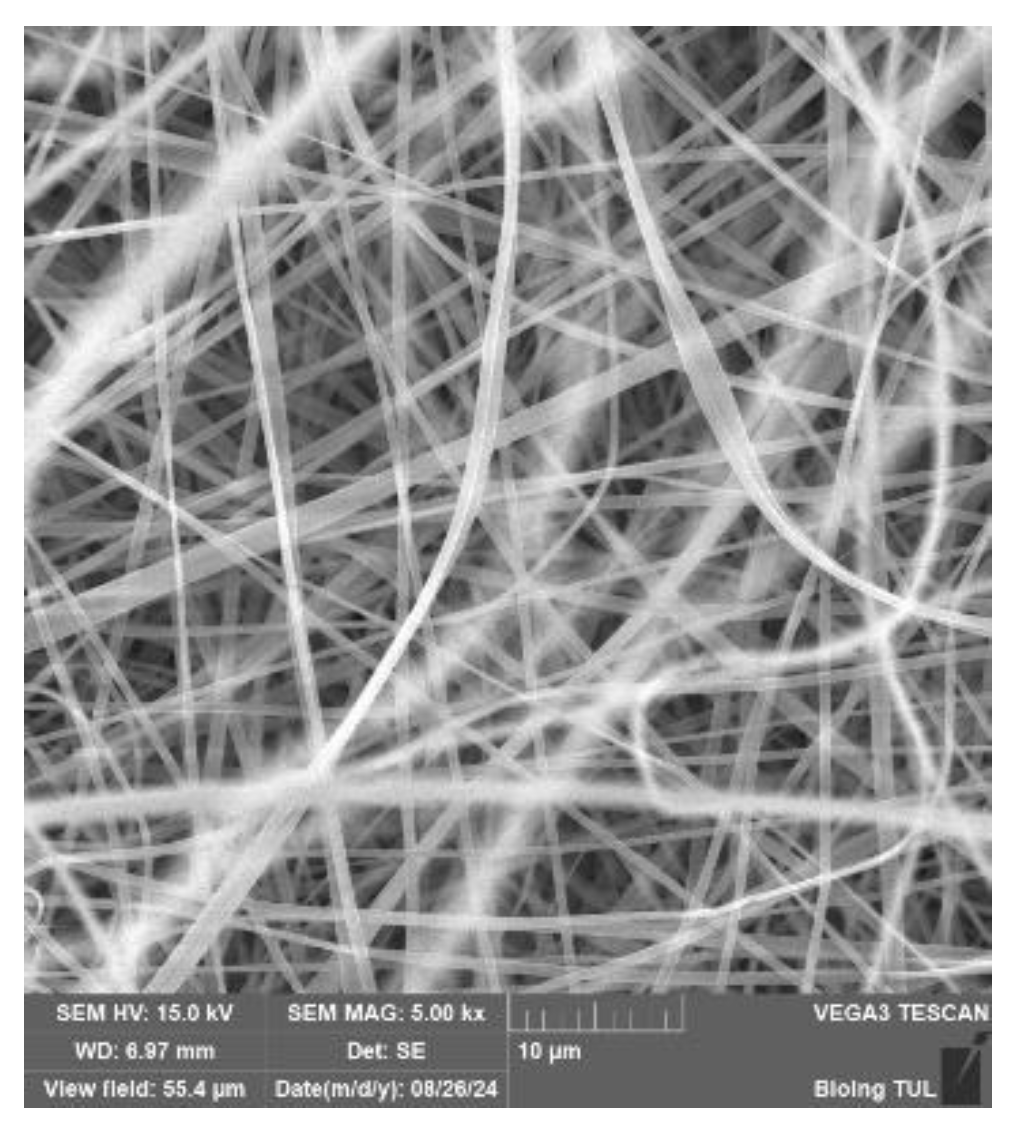
SEM analysis of PVB-EL-AC nanofibre (Tesca Vegan 3 (TUL)).
Figure 32.
SEM analysis of PVB-EL-AC nanofibre (Tesca Vegan 3 (TUL)).
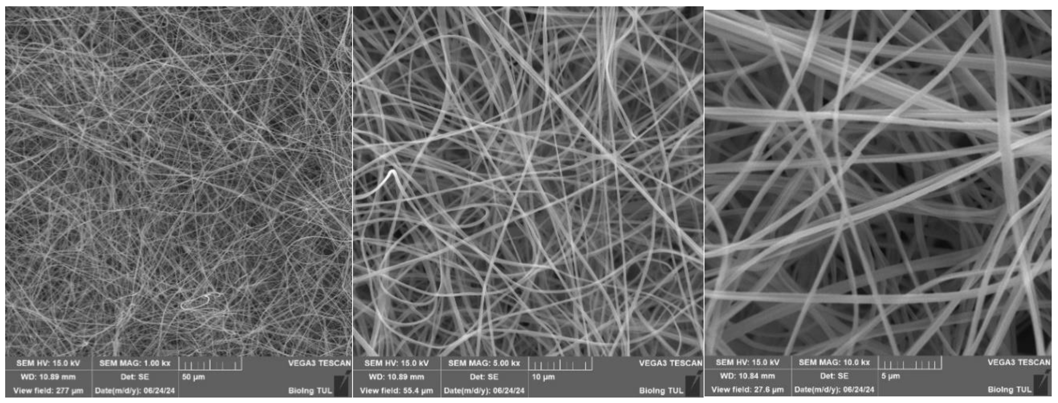
Figure 33.
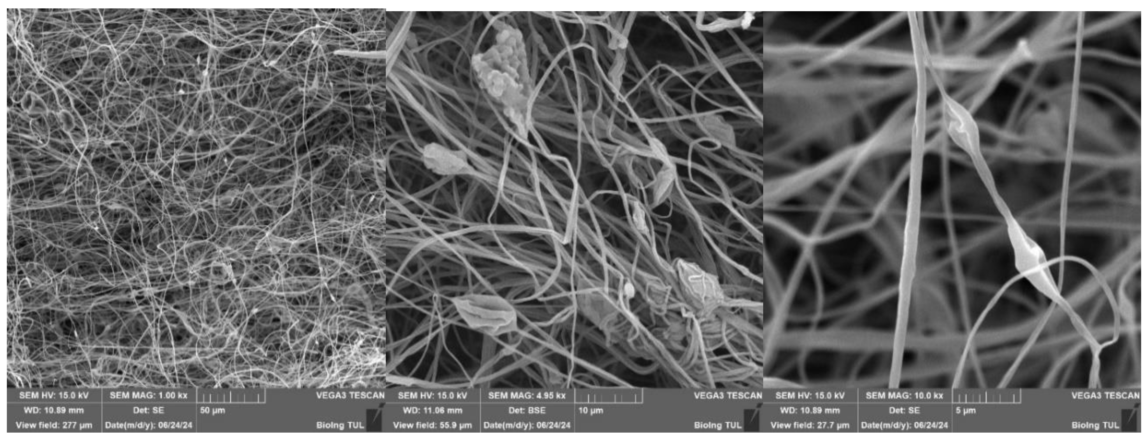
SEM analysis of PVB nanofibers with g-C3N4 EL-AC; A – magnification 50 μm; B – magnification 10 μm; C – magnification 5 μm (Tesca Vegan 3 (TUL)).
Figure 33.
SEM analysis of PVB nanofibers with g-C3N4 EL-AC; A – magnification 50 μm; B – magnification 10 μm; C – magnification 5 μm (Tesca Vegan 3 (TUL)).
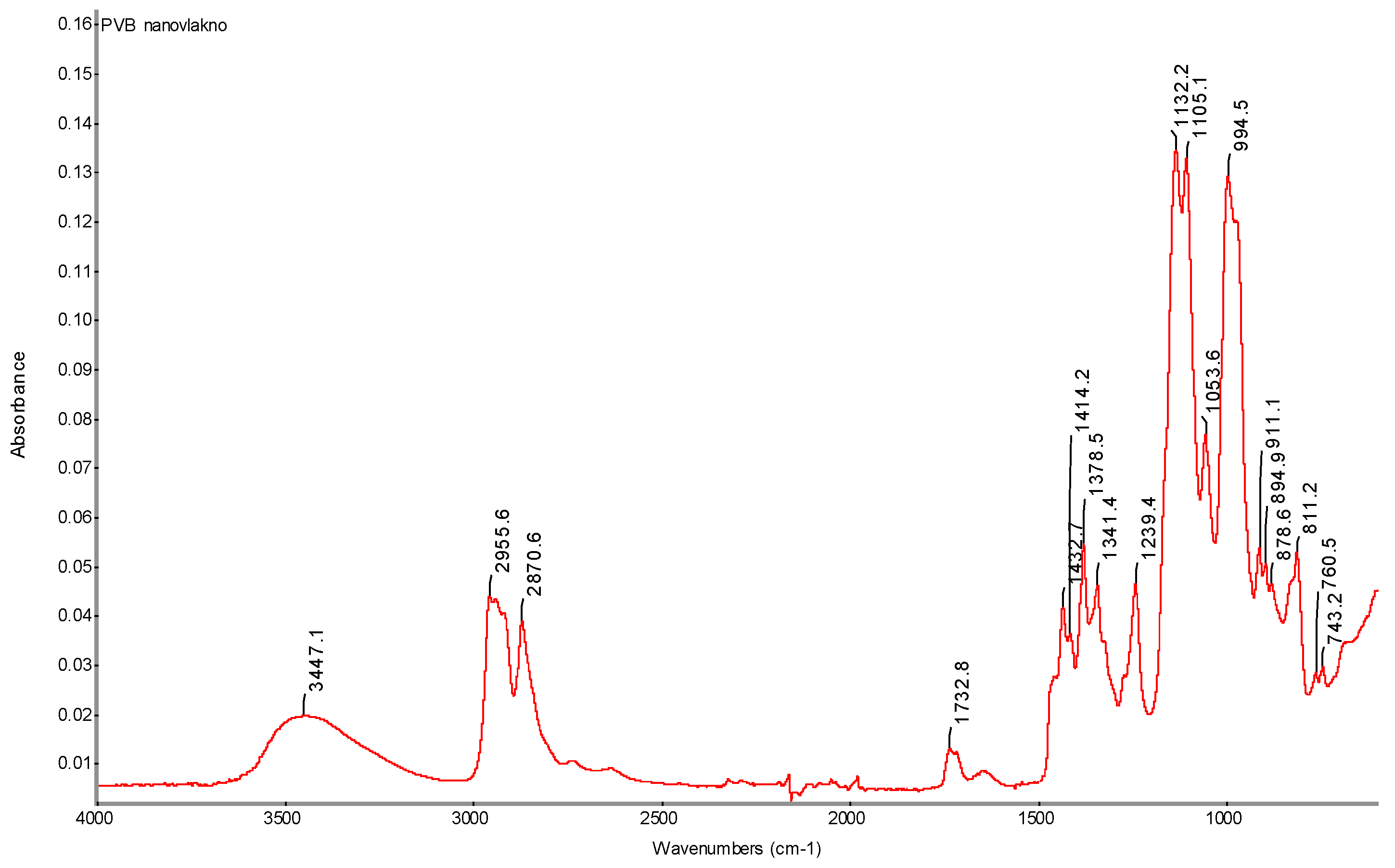
Figure 34.
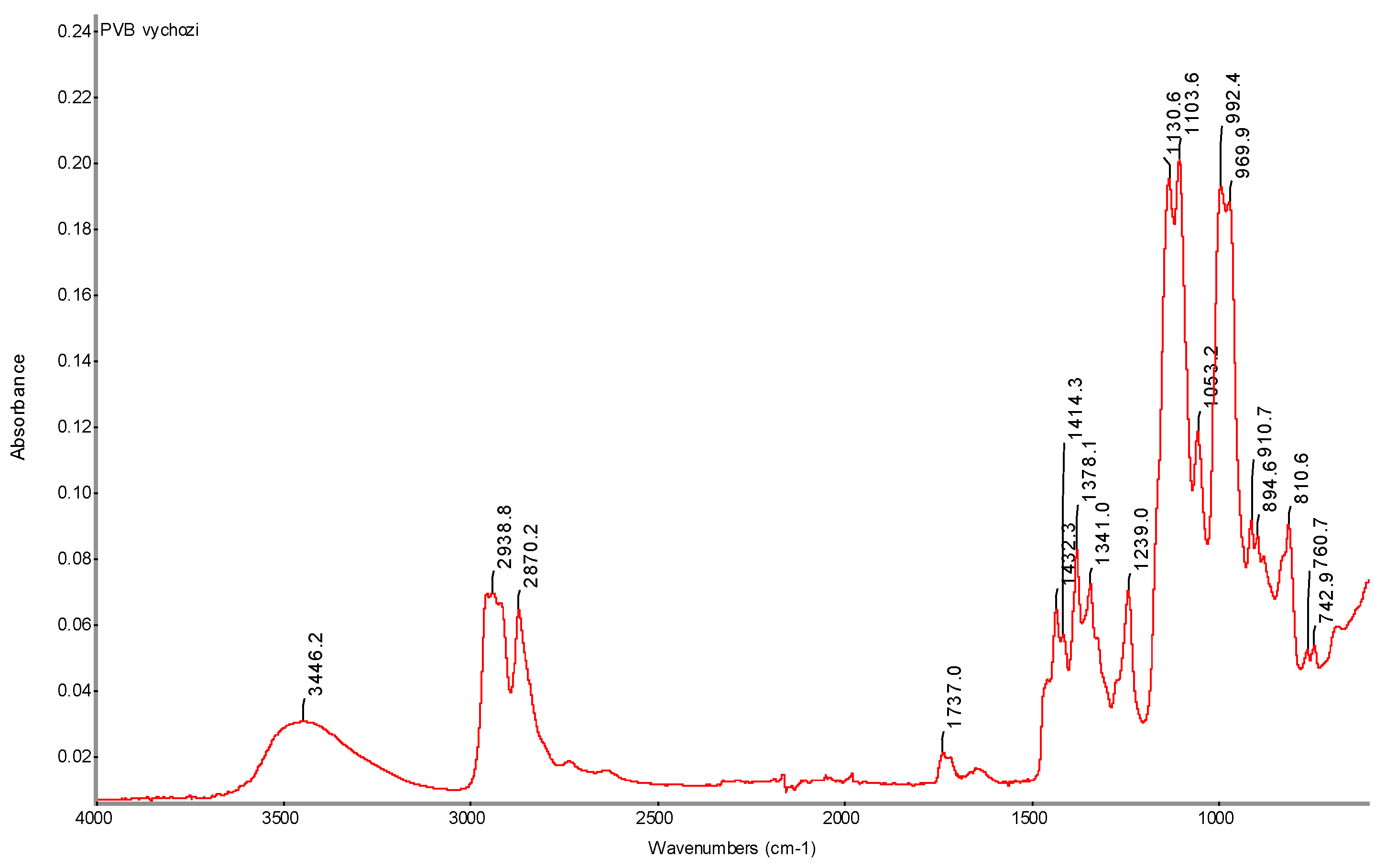
FTIR spectrum of initial PVB powder with determination of characteristic bands.
Figure 34.
FTIR spectrum of initial PVB powder with determination of characteristic bands.
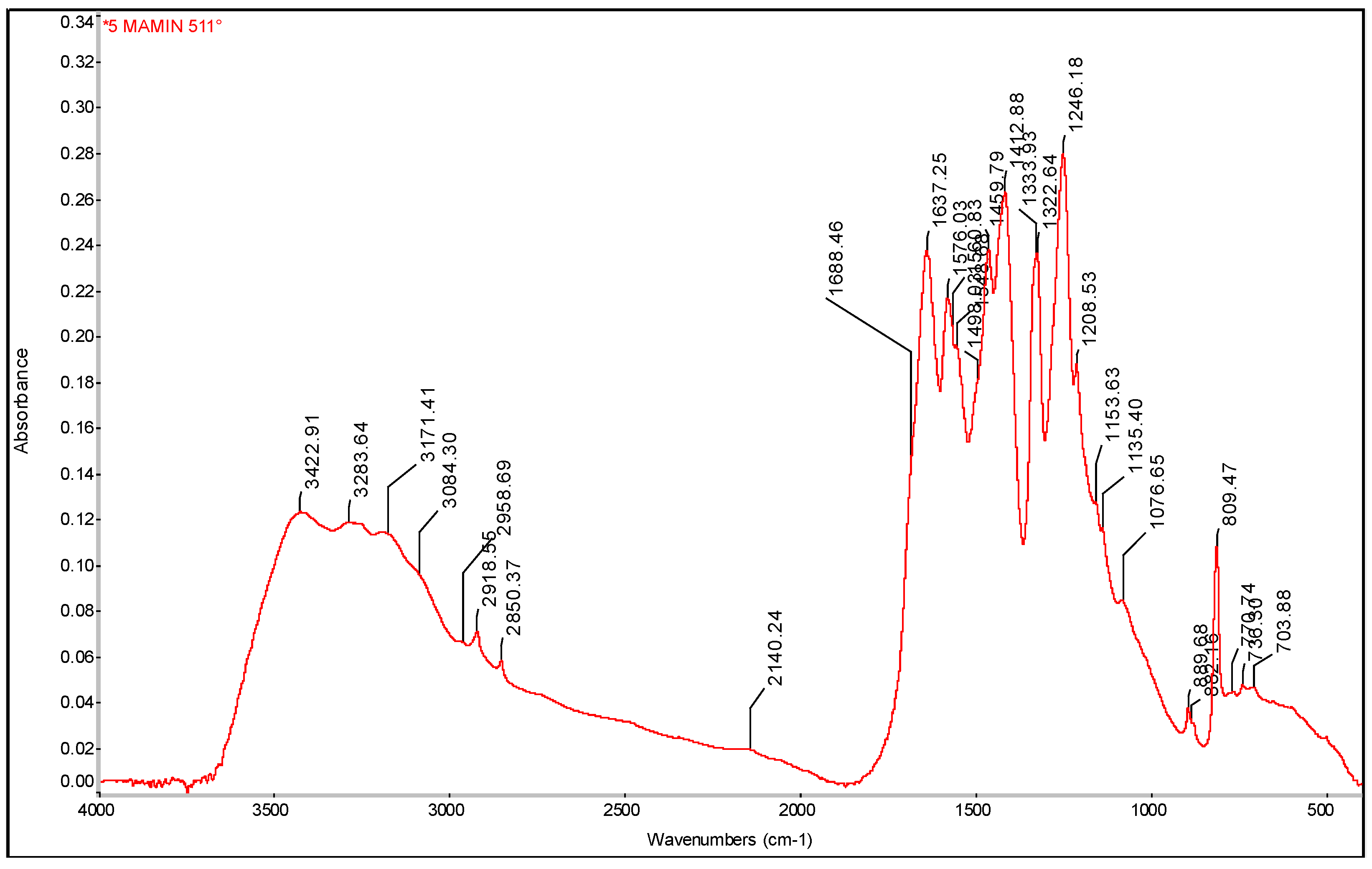
Figure 35.
FTIR spectrum of pure PVB nanofibers with determination of characteristic AC electrospinning bands (AC-EL).
Figure 35.
FTIR spectrum of pure PVB nanofibers with determination of characteristic AC electrospinning bands (AC-EL).
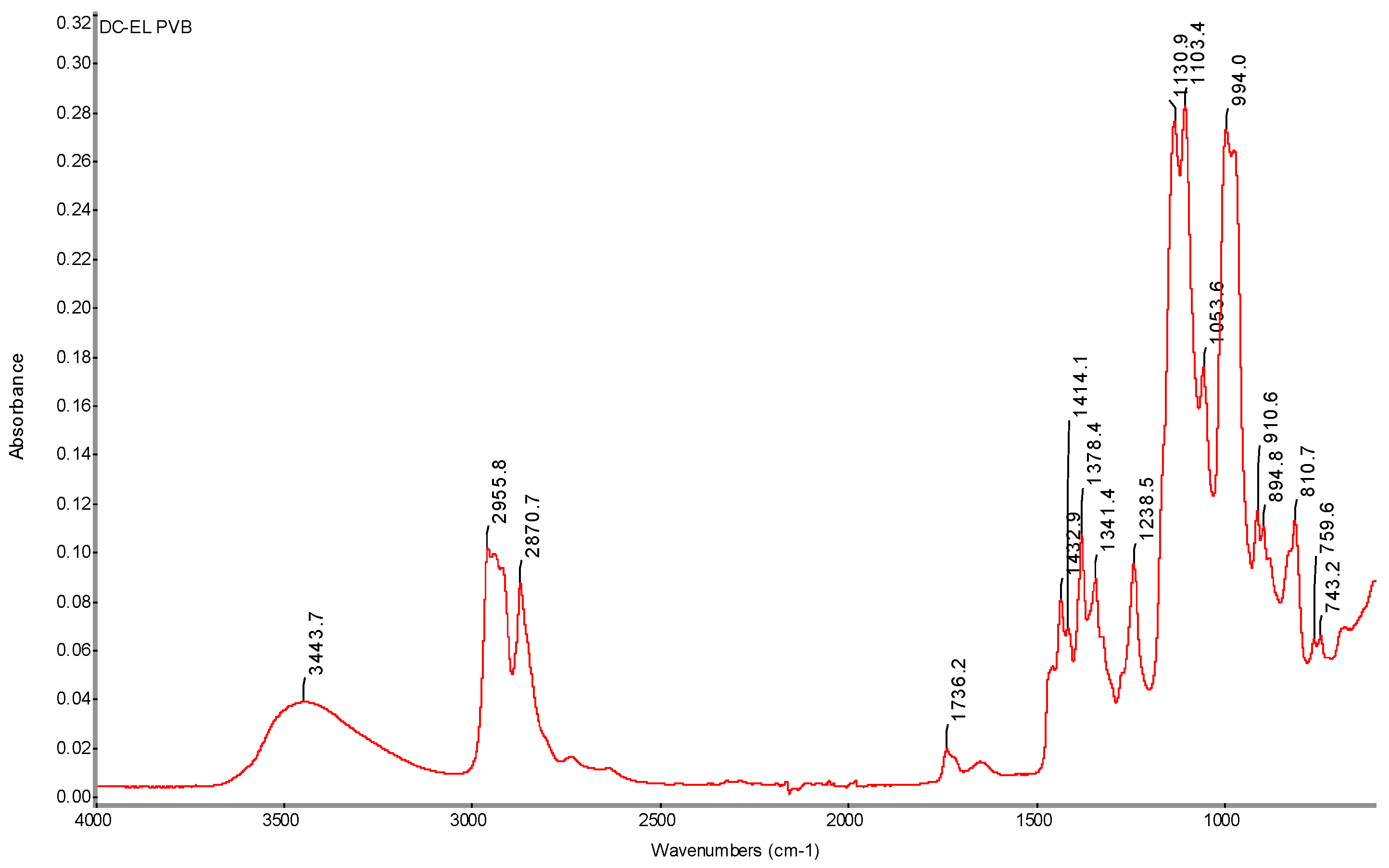
Figure 36.
FTIR spectrum of pure PVB nanofibers with determination of characteristic DC electrospinning bands (DC-EL).
Figure 36.
FTIR spectrum of pure PVB nanofibers with determination of characteristic DC electrospinning bands (DC-EL).
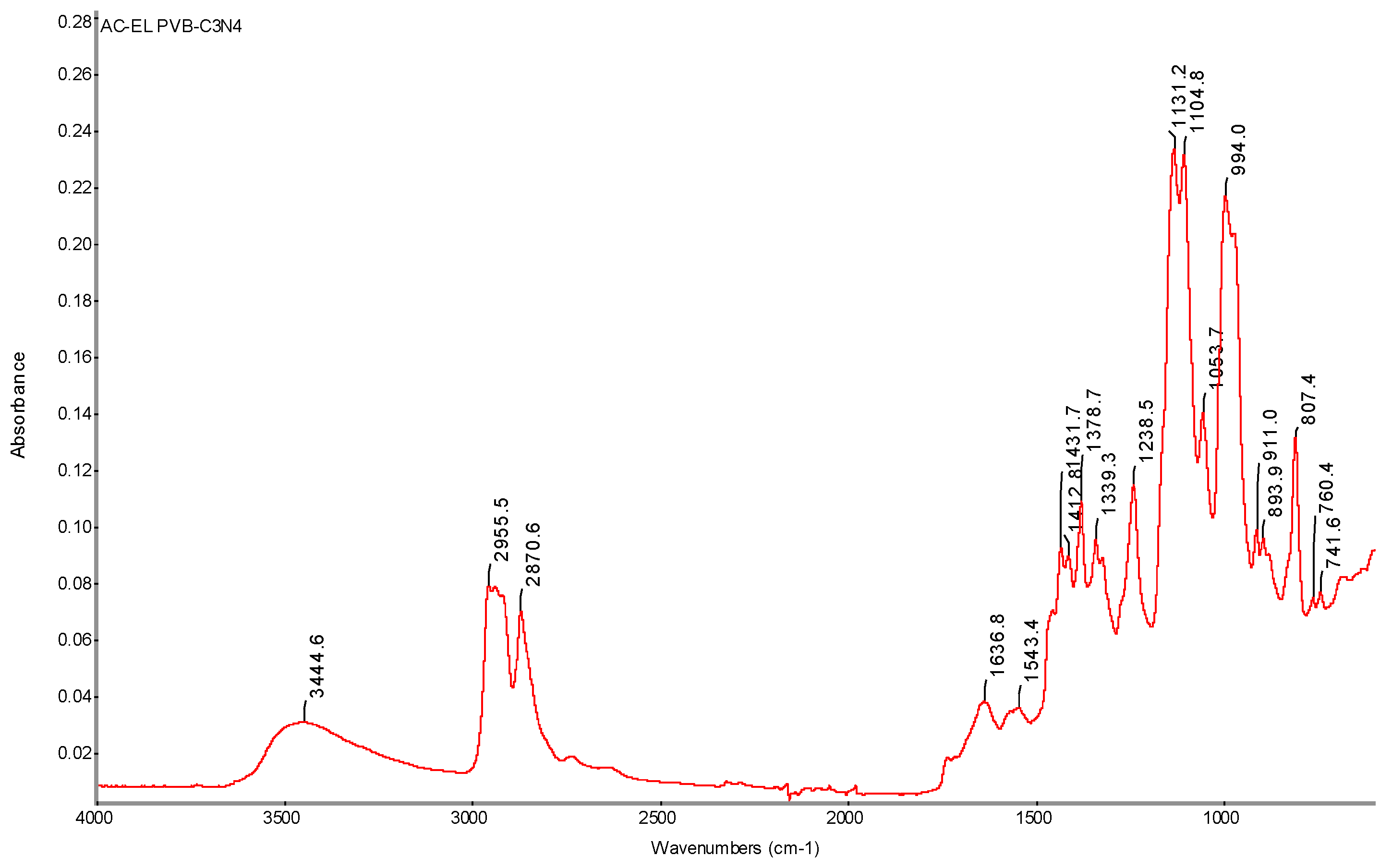
Figure 37.
FTIR spectrum of nanofiber sample with PVB-C3N4 AC electrospinning (AC-EL) with determination of characteristic bands.
Figure 37.
FTIR spectrum of nanofiber sample with PVB-C3N4 AC electrospinning (AC-EL) with determination of characteristic bands.
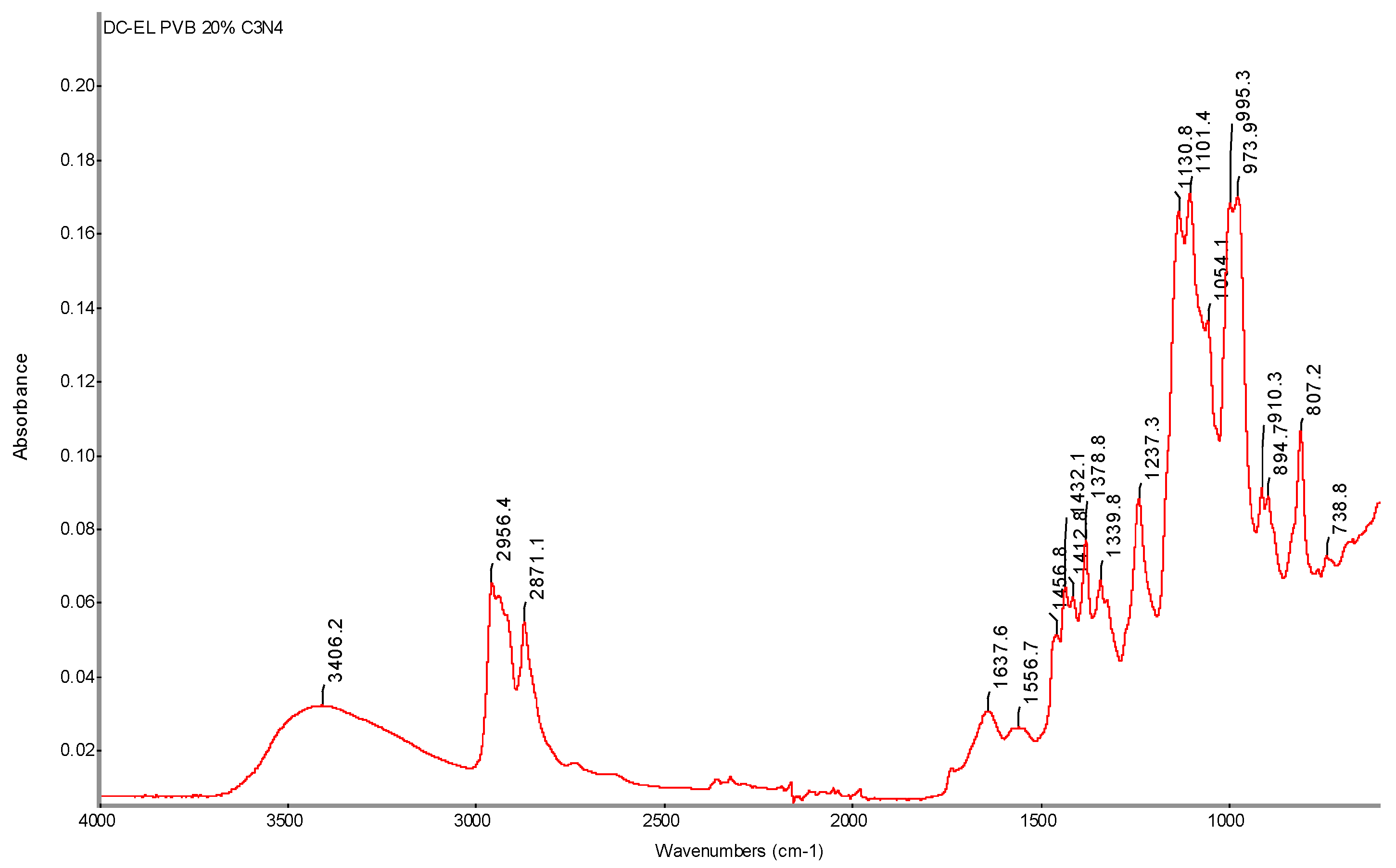
Figure 38.
FTIR spectrum of PVB 20% C3N4 DC-EL nanofiber sample with determination of characteristic bands.
Figure 38.
FTIR spectrum of PVB 20% C3N4 DC-EL nanofiber sample with determination of characteristic bands.
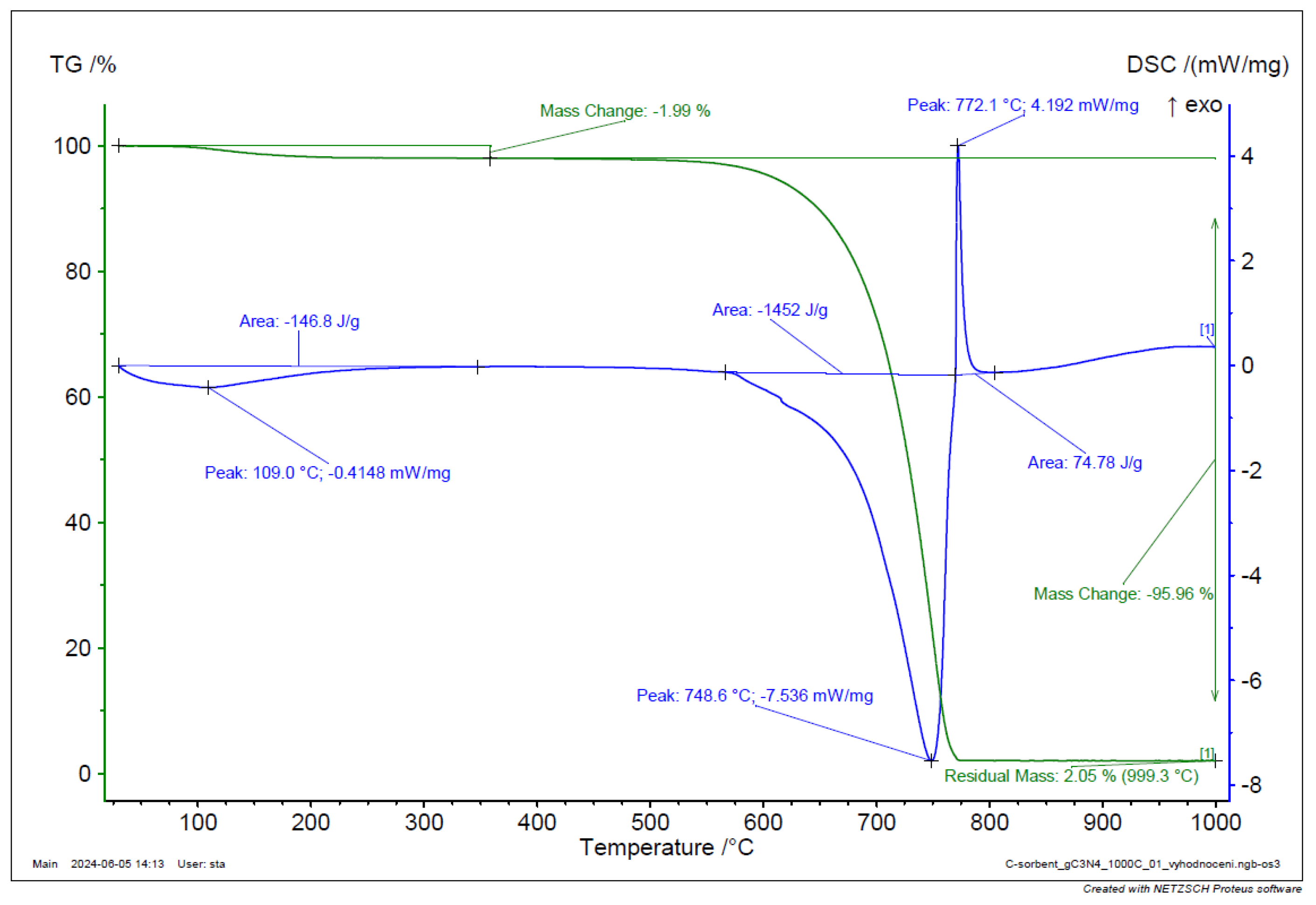
Figure 39.
TGA and DSC analysis of g-C3N4 sample.
Figure 39.
TGA and DSC analysis of g-C3N4 sample.
Figure 40.
TGA and DSC analysis of PVB EL-DC nanofiber.
Figure 40.
TGA and DSC analysis of PVB EL-DC nanofiber.
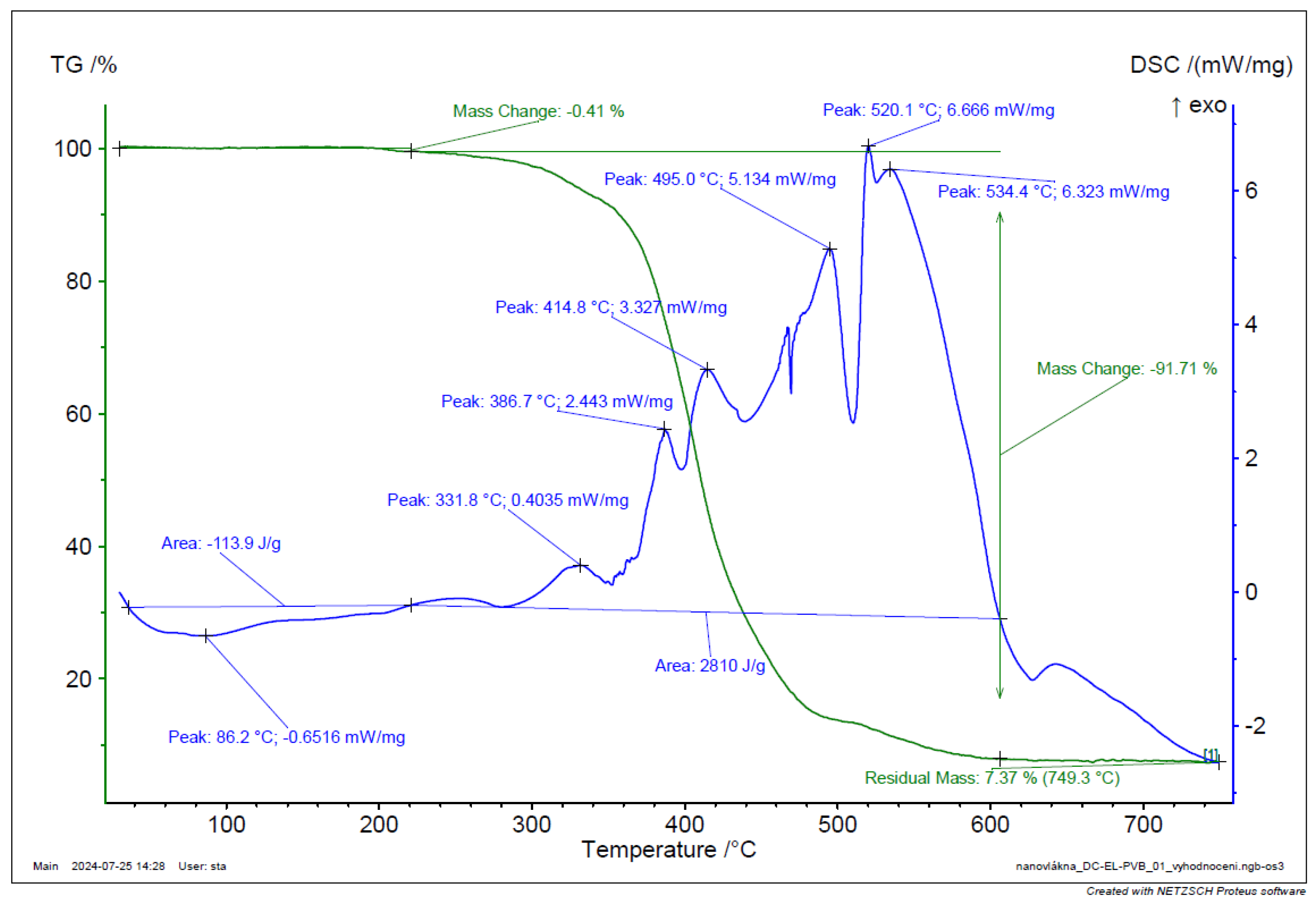
Figure 41.
TGA and DSC analysis of PVB-C3N4 EL-DC nanofiber.
Figure 41.
TGA and DSC analysis of PVB-C3N4 EL-DC nanofiber.
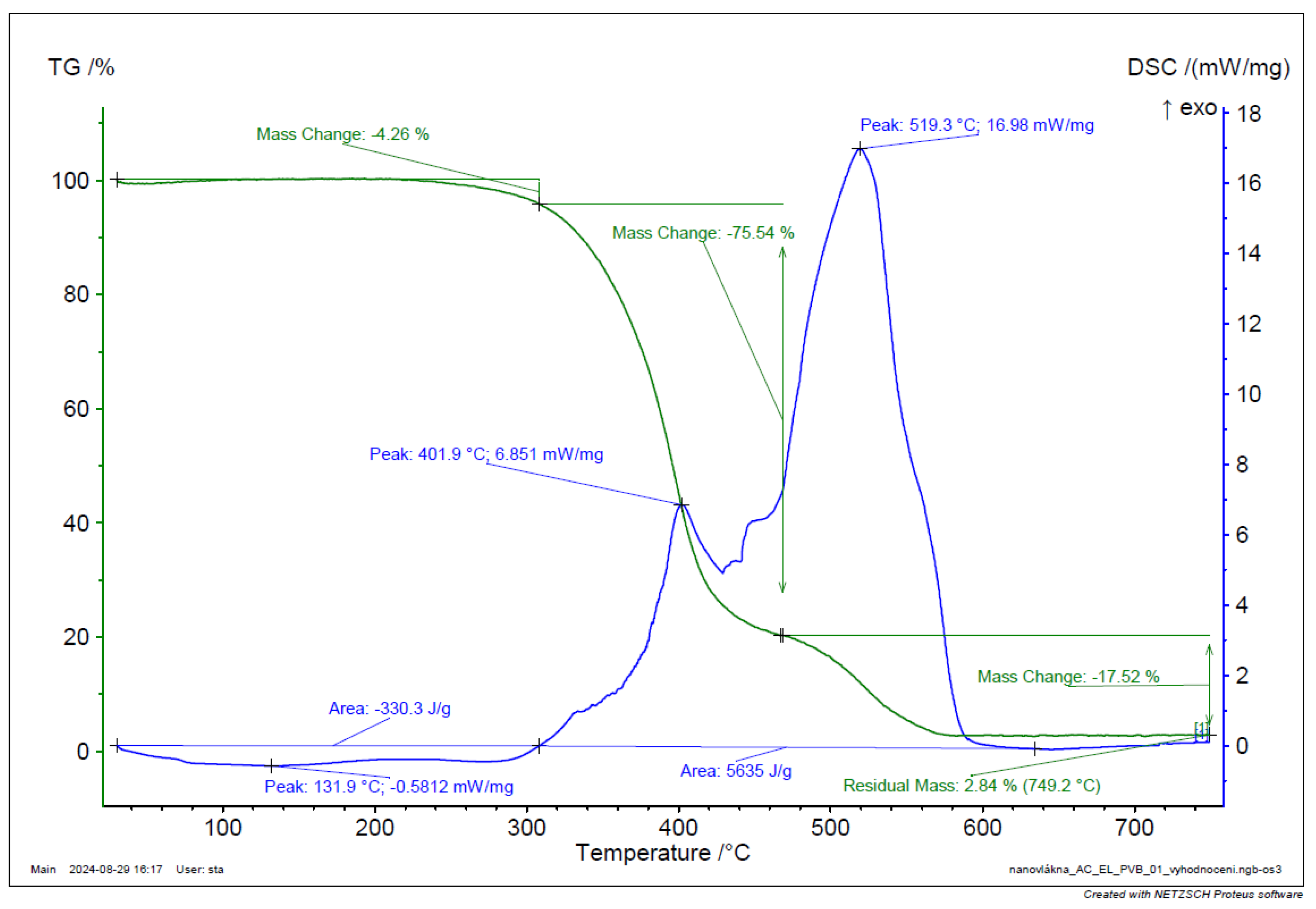
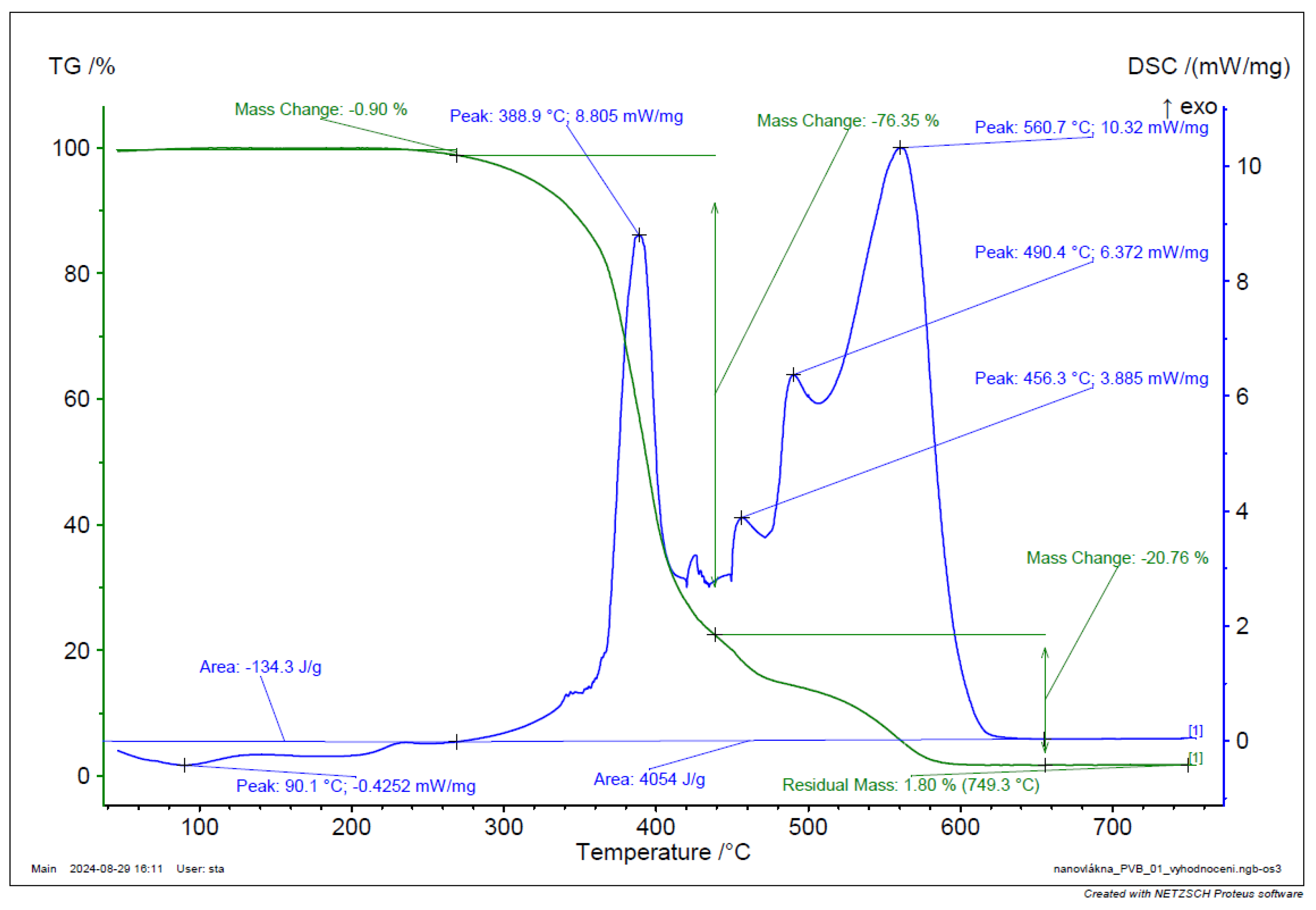
Figure 42.
TGA and DSC analysis of PVB EL-AC nanofiber.
Figure 42.
TGA and DSC analysis of PVB EL-AC nanofiber.
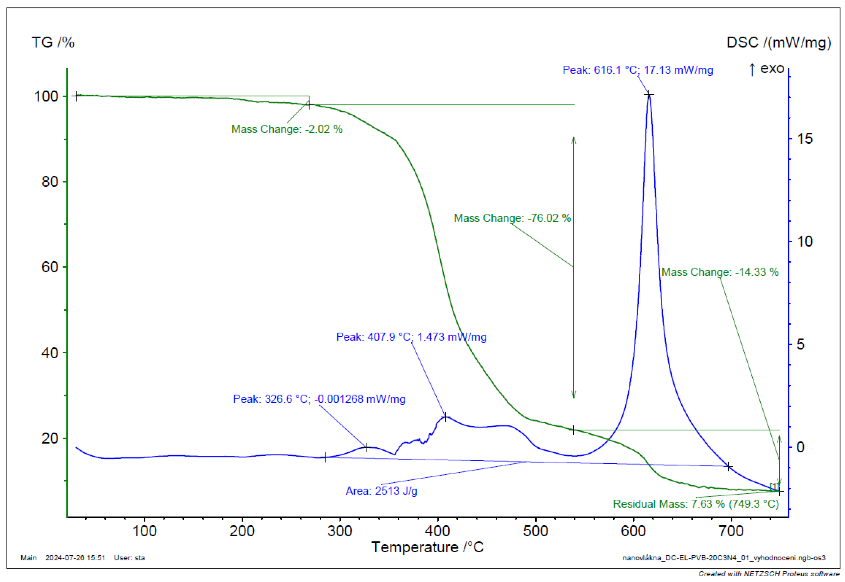
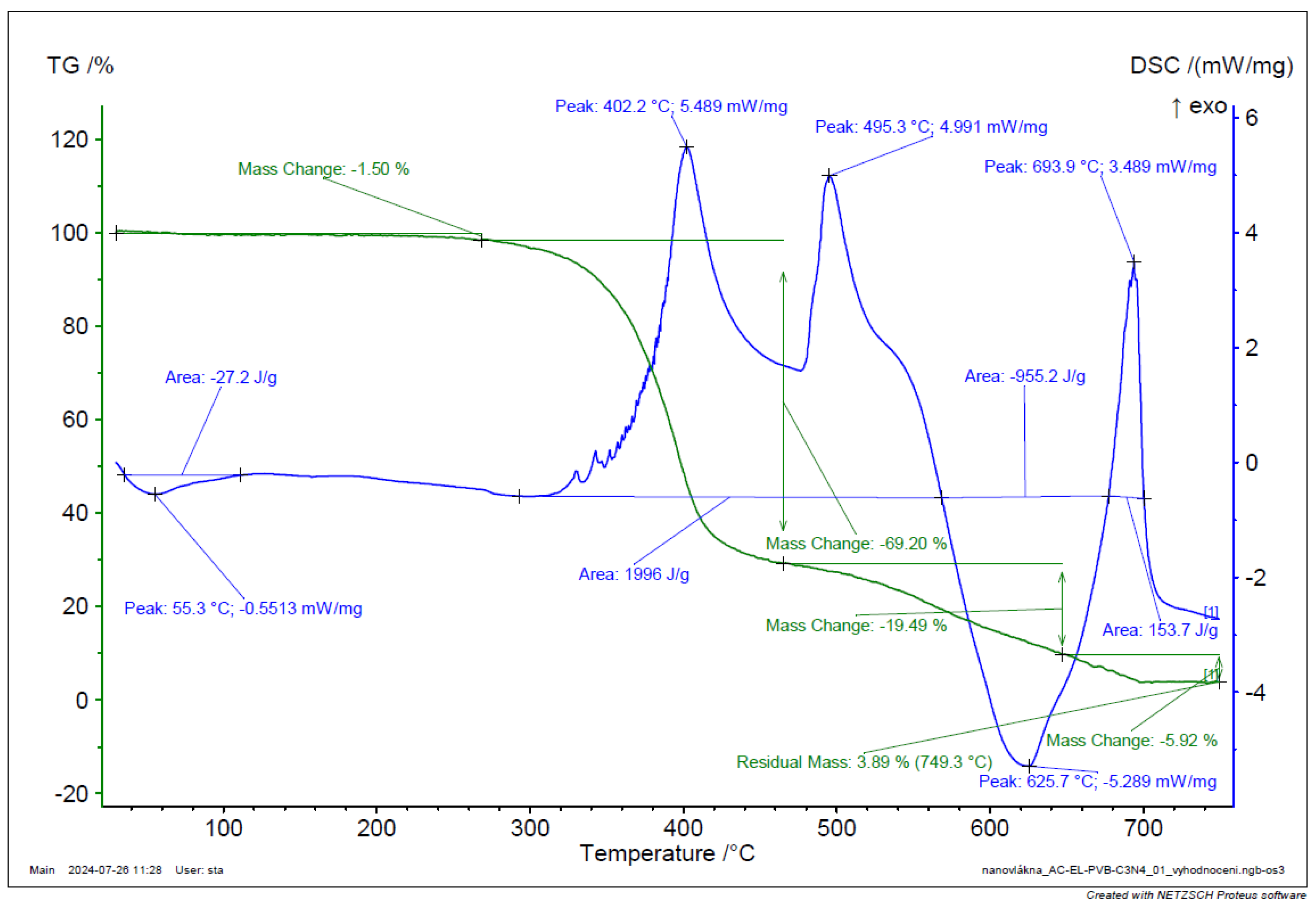
Figure 43.
TGA and DSC analysis of PVB-C3N4-EL-AC nanofiber.
Figure 43.
TGA and DSC analysis of PVB-C3N4-EL-AC nanofiber.
Figure 44.
TGA and DSC of PVB powder.
Figure 44.
TGA and DSC of PVB powder.