Leveraging Generative AI for Modelling and Optimization of Maintenance Policies in Industrial Systems

1. Introduction

Maintenance policies have long been a critical component of industrial asset management, ensuring that systems continue to operate efficiently while minimizing downtime and operational costs. Traditional maintenance approaches—ranging from corrective maintenance (performed after failures) to preventive strategies like age- or condition-based maintenance—have evolved to include more sophisticated models that optimize resource use, asset reliability, and cost efficiency. The optimization of these maintenance policies has typically been driven by well-established mathematical models and simulation techniques. These models are often designed to minimize expected maintenance costs over a finite period while ensuring that reliability, operational and eco efficiency targets are met [25].

However, while effective, these traditional approaches may be limited in flexibility and adaptability, often requiring manual intervention and domain expertise for adjustment and re-formulation [19].

The advent of generative artificial intelligence (AI) introduces new possibilities to the optimization and management of maintenance policies. Unlike traditional AI, which often focuses on pattern recognition and predictive analysis, generative AI can interpret, modify, and even generate new models of optimization based on industry-standard frameworks. This ability to understand and build upon existing optimization models allows for dynamic problem-solving, enhancing both the formulation of maintenance strategies and their real-time application [14,9].

Generative AI not only helps optimize maintenance policies but also offers a suite of other capabilities. It can adapt existing models to specific constraints, explore alternative formulations for finite or infinite time periods, and generate insightful visualizations of the output, allowing decision-makers to better understand the implications of various maintenance strategies [3]. Moreover, AI-assisted models can suggest innovative ways to overlap different policies, combining and creating hybrid strategies tailored to specific operational needs [3]. Therefore, the novelty of this research lies in the application of generative AI to dynamically model, optimize, and interact with maintenance policies. Specifically, the research demonstrates how generative AI can:

• Understand and re-formulate traditional maintenance models: Instead of simply optimizing predefined models, generative AI can adapt, restructure, and improve models based on real-time data or shifting operational needs [14].
• Combine multiple policies dynamically: It offers a unique capability to overlap various maintenance strategies (e.g., preventive overhauls, corrective interventions, minimal repairs, imperfect maintenance, etc.), creating hybrid strategies that are more adaptable to industrial complexities [3].
• Offer enhanced interaction with optimization models: By enabling users to interact with the AI, it allows for adjustments not just in policy but also in the visualization of outcomes, the re-formulation of the model in finite time periods, and other exploratory tasks that go beyond traditional optimization techniques [3].
• Real-time adaptability: The AI’s ability to learn and refine strategies dynamically allows for real-time problem-solving in maintenance operations, unlike static models that require frequent manual updates [14].

This integration of generative AI with maintenance policy optimization represents a novel approach to industrial asset management, providing greater flexibility, deeper insights, and more comprehensive solutions to complex maintenance challenges.

2. The Maintenance Policy Concept

In the context of maintenance and dependability standards, such as IEC Electropedia 192-06-02:2015, a maintenance policy is a comprehensive framework that delineates maintenance objectives, lines of maintenance, indenture levels, maintenance levels, maintenance support, and their interrelationships. Maintenance objectives articulate the goals and desired outcomes of maintenance activities, such as maximizing uptime or minimizing costs. The line of maintenance specifies the organizational segment responsible for executing maintenance activities. Indenture levels define the hierarchical structure of system components and sub-components, which influences maintenance execution at various levels. Maintenance levels categorize different types of maintenance activities, including routine, intermediate, and depot-level maintenance. Maintenance support encompasses the necessary resources and infrastructure, such as tools, personnel, and spare parts, required to conduct maintenance activities. In academic literature, however, a maintenance policy is often more narrowly defined as a set of predefined rules and strategies that dictate how maintenance activities are conducted on a system, whether single-unit or multi-unit, to ensure its reliability and operational efficiency [2,21,28,6,11,8,4,24].

Some examples of this, for a single unit, are the following:

• The age-dependent preventive maintenance (PM) policy for a single unit system is a common approach where a unit is replaced at a predetermined age T or upon failure, whichever occurs first [2]. This policy has evolved to include concepts like minimal, imperfect or perfect repair for CMs [30], or imperfect maintenance for PMs [30,15,7] leading to various extensions and modifications (failure limit policy, failure cost limit policy, etc.).
• A very useful extension of previous policies was the partial replacement policy [16], that is based on the idea that in most cases where a system fails, a full replacement of the system is not necessary to restore it to proper operating conditions. Instead, a partial preventive replacement (PPR) of some components is sufficient. PPRs are interventions, many times named overhauls in industry, performed when the system reaches a certain age, which restore the system’s failure rate to its initial level. After a certain number of partial preventive replacements (to be determined), the accumulated costs of these interventions may exceed the cost of performing a total replacement of the system.
• Random age-dependent maintenance policy addresses scenarios where it is impractical to maintain a unit on a strictly periodic basis. Instead, maintenance is performed at random intervals, taking advantage of available free time [4,28]. In this context, a unit’s age is measured from the time of the last replacement, and minimal repairs are undertaken upon failure, leading to a periodic replacement with minimal repair at failure policy.
• Recently, [19] introduce an imperfect maintenance policy that defines a reliability improvement factor according to the intervention level of maintenance actions. This assumes the intervention level to be independent of the time between consecutive maintenance actions, removing the common constraint that longer intervals necessitate higher intervention levels. Additionally, it optimizes not only the number of maintenance activities, their timing, but also the intervention levels of maintenance activities

While maintenance policies for single-unit systems focus on the timing and type of maintenance actions to ensure reliability and operational efficiency, multi-unit systems introduce additional complexity due to the interdependence between units. This interdependence necessitates a coordinated approach to maintenance, considering the hierarchical structure of components, redundancy, and the interactions between different units. These policies are designed to address the specific challenges of multi-unit systems as a whole, including efficiently managing redundancy and spare parts.

Some examples of this, for a single unit, are the following:

• Group Maintenance: Maintenance is conducted simultaneously on a group of units to reduce costs and downtime [6,25].
• Selective Maintenance: Maintenance prioritizes specific units based on their criticality or condition to optimize overall system reliability [31].
• Condition-Based Maintenance (CBM): Maintenance schedules are based on real-time monitoring of unit conditions, adapting to the varying states of different units [30,27,29,10].
• Opportunistic Maintenance: Maintenance takes advantage of planned downtimes or failures of one unit to perform maintenance on other units, minimizing overall downtime and costs [28,12].

Single-unit and multi-unit maintenance policies also account for different types of cost structures, that can be dependent of age, number of PMs and/or number of CMs, can be neglecting, or not, times for maintenance, considering or not penalties, residual value of the unit, etc.

For the purposes of this paper, we will adopt the more focused definition of a maintenance policy as described in the academic literature. This includes the specific strategies for performing maintenance actions based on the age and condition of the unit, incorporating preventive and corrective maintenance actions, considering total or partial replacements and various degrees of repair and PM. Also, we will focus on single-unit systems, with the intention of further similar investigation in multi-unit ones.

3. Criteria for Maintenance Policies Optimization

One of the most prevalent optimization criteria in maintenance policies is the minimization of costs. This criterion involves reducing the total expected cost of maintenance over a specified period, considering both preventive and corrective maintenance actions. For example, in the age-dependent preventive maintenance policy discussed by [2], the goal is to find the optimal replacement age TT that minimizes the combined cost of scheduled replacements and unscheduled failures. Similarly, [6] focus on minimizing maintenance costs by determining the optimal intervals for preventive maintenance and the degree of repair required after failures.

Another important optimization criterion is the maximization of system reliability and availability. This involves ensuring that the system operates without failures for as long as possible, thereby increasing its uptime and reducing downtime. [30] emphasize the importance of reliability in their models, incorporating concepts of minimal, imperfect, and perfect maintenance to optimize maintenance schedules and actions. These policies are critical in environments where operational continuity is essential. Policies are optimized to ensure that maintenance activities cause minimal disruption to production processes. This involves strategic scheduling of maintenance tasks during non-peak hours or integrating predictive maintenance techniques to anticipate and prevent failures before they occur [26,5].

In some cases, optimization criteria also include risk and safety considerations. This involves ensuring that the maintenance policy not only minimizes costs and maximizes reliability but also reduces the risk of catastrophic failures and ensures the safety of operations. [28] highlight the importance of considering the risk of failure and the potential consequences in their maintenance models. By incorporating risk and safety factors, they aim to develop maintenance policies that are not only cost-effective but also safe and reliable. Maintenance policies are designed to mitigate risks associated with equipment failures and ensure compliance with safety regulations, thereby protecting both personnel and assets [1,23].

Recent studies have highlighted the importance of considering energy consumption and greenhouse gas (GHG) emissions in maintenance policy optimization. By integrating these environmental factors, organizations aim to reduce their carbon footprint and improve sustainability. This approach often balances the trade-off between maintenance costs and environmental impact, promoting more eco-friendly maintenance strategies [25].

Some frameworks assess the long-term financial impact of maintenance policies by calculating their net present value (NPV). This approach evaluates the overall financial benefits of a maintenance policy over its lifecycle, considering both immediate costs and long-term savings. Following this criterion, organizations can justify maintenance investments that offer significant returns over time [13].

Finaly, there is always the possibility of using a multi-criteria decision-making models, incorporating several criteria simultaneously. These models help in developing maintenance policies that optimize multiple objectives, ensuring a more balanced and comprehensive approach. For instance, the use of MCDM allows maintenance managers to prioritize actions based on the criticality of equipment, potential safety hazards, and operational impact, rather than solely focusing on cost [8; 24].

For the purposes of this paper, we will use maintenance policy optimization criteria based on improving the expected total cost of the policy. This approach does not preclude the possibility of conducting the same study using other optimization criteria, ensuring the generality of our findings.

4. The Problem Statement

The idea of this section is to investigate some distinct use cases where Generative AI can deliver actionable insights, optimize maintenance plans, and facilitate the assessment of performance enhancements. Through a rigorous examination of varied prompts, we aim to demonstrate the capacity of Generative AI not only to streamline existing processes but also to contribute to the ongoing refinement of maintenance strategies.

For this exercise we use the CHAT GPT-4o [17] as the chatbot or conversational AI system, and the Jupyter Notebook, (which is a web-based, interactive computing notebook environment using with Python 3), as the open-source interactive web application to create live code, equations, visualizations, and narrative text [20].

We will be presenting chat prompts, or statements or question provided to the chatbot to initiate a conversation or request specific information or assistance. A prompt serves as an input for the AI model to generate a relevant response or carry out a particular task. Chat prompts are commonly used in natural language processing applications, chat-based interfaces, and virtual assistants to facilitate human-computer interactions. Users can input prompts to engage in a dialogue, ask questions, or seek assistance, and the AI model responds based on its training and understanding of the provided input.

After this introduction let’s continue with our prompts. The idea when building the prompts is to arrive to a formulation that generate a suitable answer when prompted. This is sometimes not an easy task. The user must make sure that rephrasing the prompt, containing the similar structured information, the answer is similar.

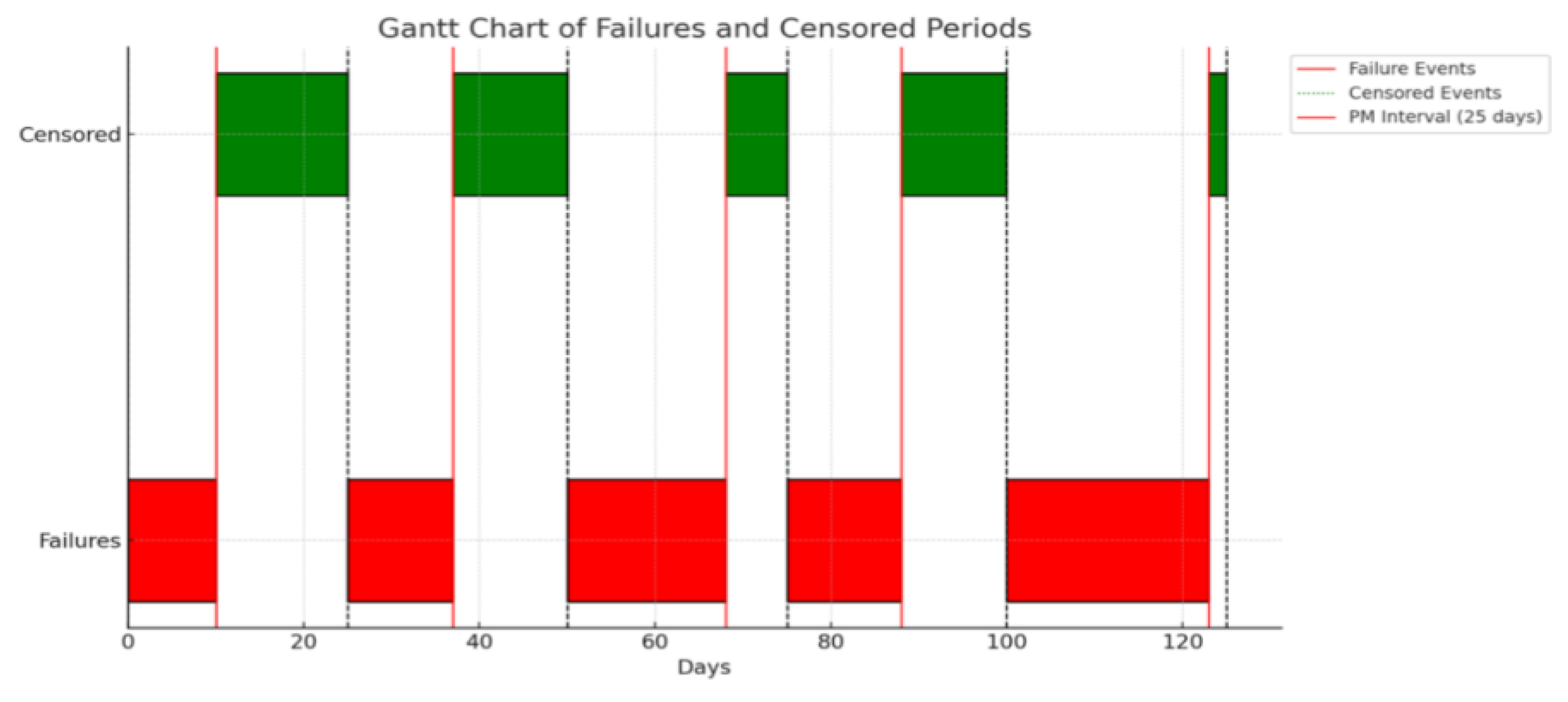
In a first prompt we provide the chatbot the data needed for a unit reliability analysis for a given failure mode. Assuming a existing PM cycle (25 calendar days), and before questioning about the adequacy of that policy. Therefore, this first prompt is only to explore the failure behavior. Notice that the number of total days of operation is not needed (redundant data). Also, we are not questioning the goodness of the fit to save space in the Section. The prompt is as follows:

• Prompt 1. Fitting the failure data to a Weibull distribution using the MLE.

Suppose we are operating a component, under the assumption that this component maintenance program is in place, employing a calendar-based schedule with a preventive maintenance (PM) cycle of 25 calendar days, this program was decided according to initial guesstimates about preventive and failure/corrective operations’ cost. Additionally, we are assuming there is no significant downtime for either preventive or corrective maintenance, or, in other words, we disregard it in comparison to the time between maintenance operations. After 120 days of operation (starting Jan 1st), a specific number of failure incidents (measured in operating time to failure in days) and preventive replacements (measured in operating time to replacement in days) have been recorded.

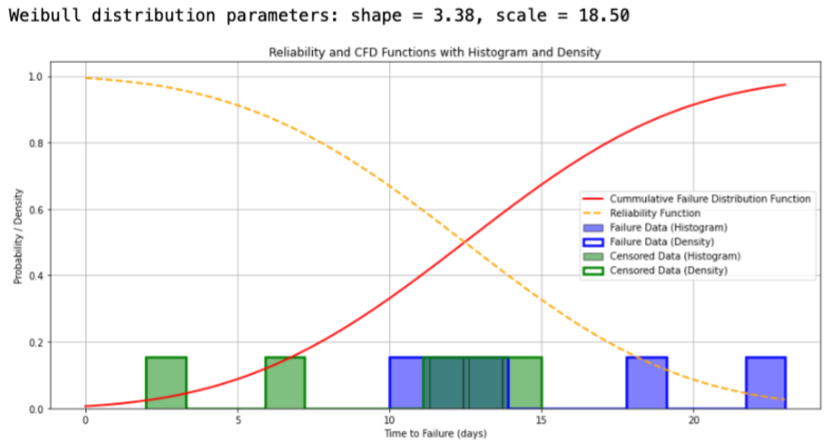
The total days of operation (125) is the sum of all the times recorded. Prior to questioning the appropriateness of our current PM cycle (25 calendar days), we have opted to investigate the failure behavior. Failure data (time to failure data) is: 10, 12, 18, 13 and 23. Censored data (time to preventive maintenance) is: 15, 13, 7, 12 and 2. With this data we would like to generate a histogram of failure and censored data (in different color). Fit the Weibull distribution: Use the maximum likelihood estimator to fit a Weibull distribution to the pooled data. Interpret the results: Once the fit is complete, we print out the parameters of the Weibull fit for review and analysis. After doing the above, present the plot of the reliability and CFD functions, with the time to failure, x of the graph.

Figure 1. Graphical representation of the scenario description as in Prompt 1.

Figure 1. Graphical representation of the scenario description as in Prompt 1.

This is the answer of the Chatbot (GPT-4o):

Here is the graph displaying the histograms and density of failure and censored data, along with the reliability and cumulative distribution functions fitted with a Weibull distribution.

• Blue: Histogram and density of failure data.
• Green: Histogram and density of censored data.
• Red Line: Reliability function.
• Orange Dashed Line: Cumulative distribution function.

The Weibull distribution parameters are:

• Shape (β): 3.38
• Scale (η
): 18.50

This visualization helps in understanding the data distribution and the fitted Weibull model for better maintenance scheduling and reliability analysis.

Figure 2. Graph containing the results of Prompt 1.

Figure 2. Graph containing the results of Prompt 1.

5. Optimization using Total Replacement Policies

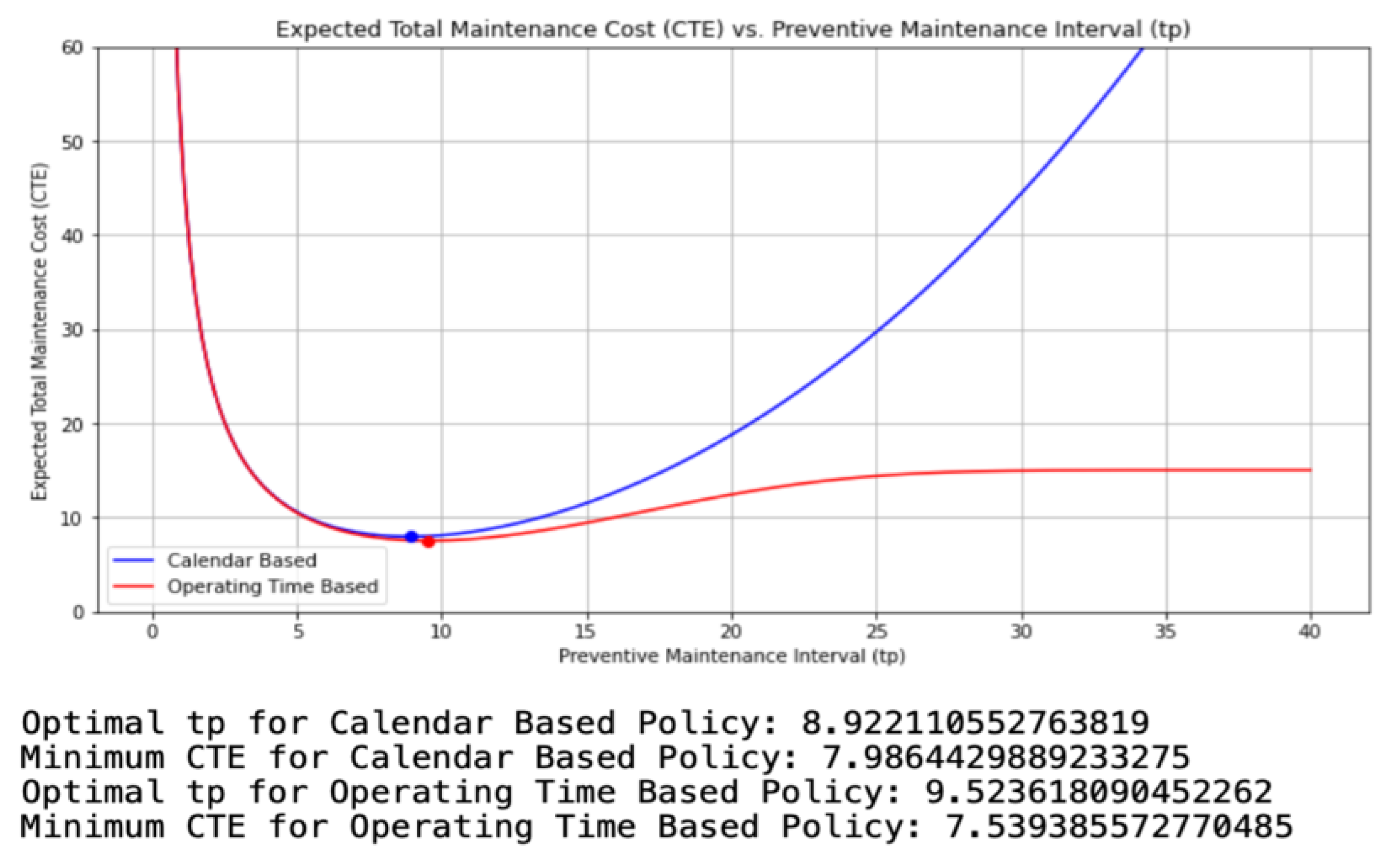
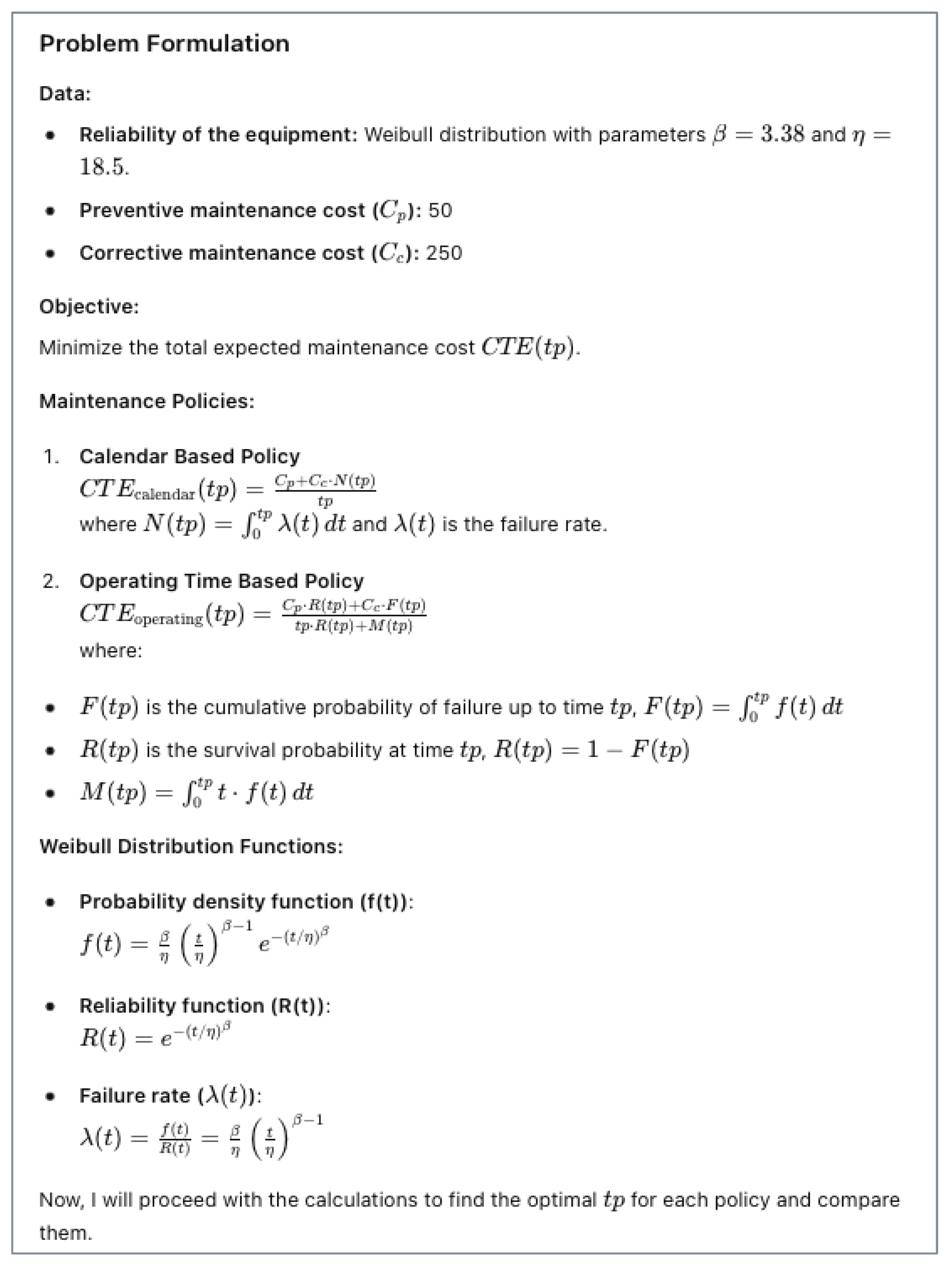
Now, let’s scrutinize the appropriateness of our existing PM cycle (25 calendar days), which necessitates a standard risk cost-benefit analysis. To facilitate this analysis, it is imperative to incorporate information pertaining to costs. In addition to this, we need to state the maintenance approach we want to assess and the criteria for optimization we wish to apply. We understand that accurately formulating the optimization problem mathematically is crucial. Here is the prompt:

• Prompt 2. Properly formulating the maintenance optimization problem.

Solve a maintenance optimization problem that involves determining the best maintenance policy to apply to a failure mode and the optimal preventive maintenance cycle time (tp) that characterizes that policy. Data to consider for the failure mode:

- Equipment reliability: Weibull (3.38, 18.5)

- Cp: Preventive maintenance cost = 50

- Cc: Corrective maintenance cost = 250

Optimization criterion: Minimize the expected total maintenance cost CTE (tp).

Maintenance policies to compare: Calendar-based vs. operating time-based

CTE (tp) for the calendar-based policy: CTE (tp) = (Cp + Cc * N(tp)) / tp

With N(tp) = integral of λ(t) from 0 to tp; λ(t) is the failure rate

CTE (tp) for the operating time-based policy:

CTE (tp) = (Cp * R(tp) + Cc * F(tp)) / (tp * R(tp) + M(tp))

Where:

F(tp) is the cumulative failure probability at time tp, i.e., the integral of f(t) from 0 to tp; f(t) is the probability density function of failures.

R(tp) is the survival probability at time tp, i.e., R(tp) = 1 - F(tp).

M(tp) = integral of t * f(t) from 0 to tp

The chatbot answer in Figure 3 is very interesting, we can check that the model, as used by the AI, is the correct one for each maintenance strategy, for each probability function and for the optimization criteria.

The chatbot answer in Figure 3 is very interesting, we can check that the model, as used by the AI, is the correct one for each maintenance strategy, for each probability function and for the optimization criteria.

In the successive prompt 3, we enable the tool to handle the problem resolution, referring to the anticipated outcomes that we’ve condensed for space in this section. See Figure 4 for the graph generated by the code provided by the chatbot. All this specific information is provided in the prompt, and this is the result:

• Prompt 3. Ordering to solve the maintenance optimization problem.

I concur with the formulation. Now, compute CTE(tp) for each specified policy, plot them for different tp values, and identify the tp that yields the minimum CTE value for each policy. Mark these values on the graph.

GPT-4o answer is as follows:

Figure 4. Python generated graph for the optimization problem solution.

Figure 4. Python generated graph for the optimization problem solution.

Once the tool demonstrates a solid grasp of the problem and a preferred (dominant in this case) maintenance strategy is chosen, we can explore additional potential scenarios to enhance decision-making in the event of changes in failure distribution and/or future changes in corrective maintenance costs. Here are the prompts (see graphical results in Figure 5 and Figure 6), now paying more attention to results, given a code obtention:

• Prompt 4. Gaining knowledge to face potential failure scenarios.

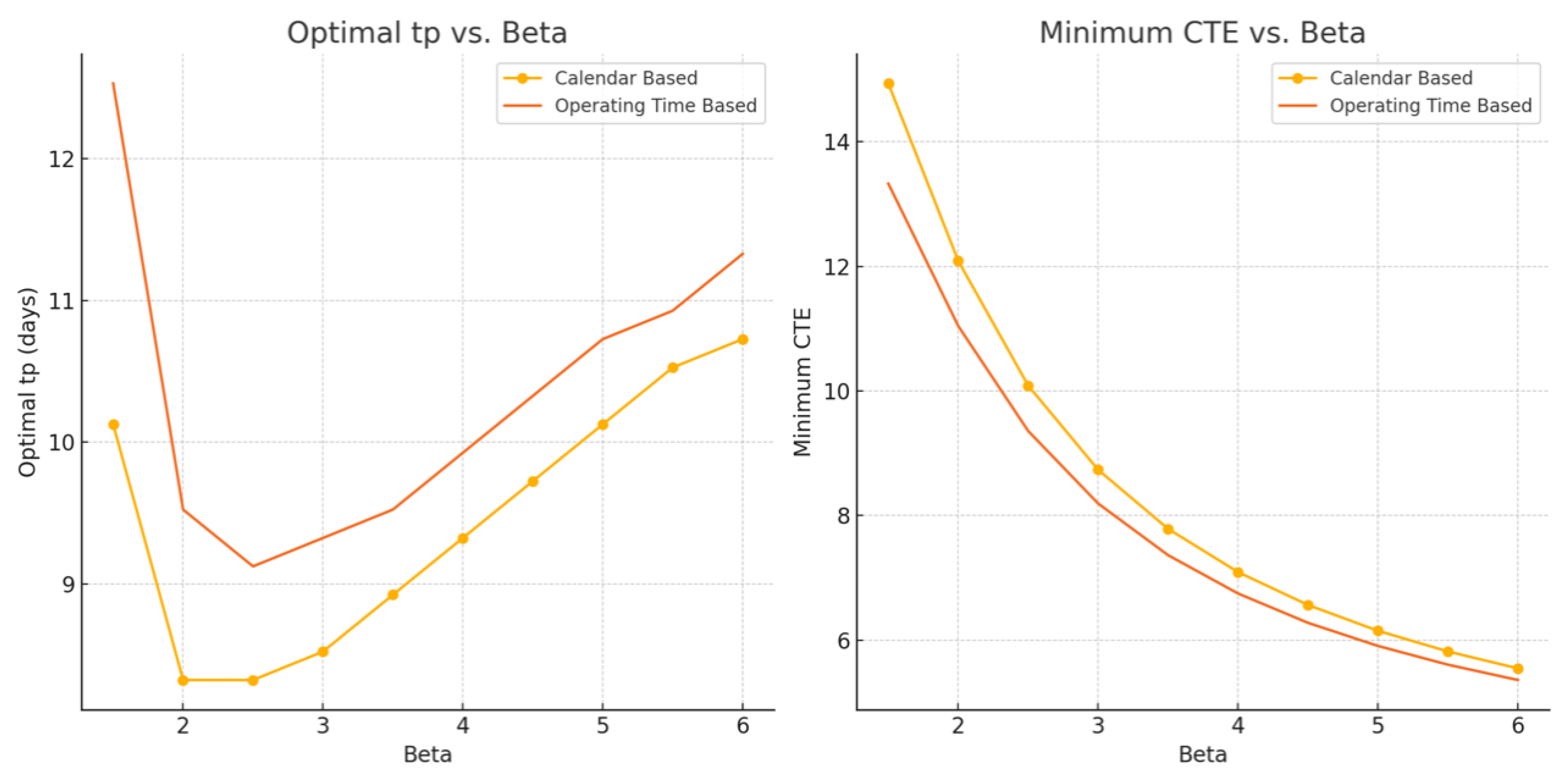
Is it possible to have a graph showing the sensitivity of these optimal intervals with respect to variations of beta values?

GPT-4o answer is as follows:

Minimum CTE vs. Beta. Here are the sensitivity analysis graphs:

• Optimal tp vs. β: This graph shows how the optimal preventive maintenance interval (tp) changes with different values of β for both calendar-based and operating time-based policies. Both policies show a decrease in optimal tp as β increases, reflecting the higher failure rates associated with higher β values.
• Minimum CTE vs. β: This graph illustrates how the minimum expected total maintenance cost (CTE) varies with different values of β. The operating time-based policy consistently results in a lower minimum CTE compared to the calendar-based policy across the range of β values.

These graphs in Figure 5 provide a clear visualization of how the optimal maintenance strategy and costs are sensitive to changes in the Weibull shape parameter (β). If you have any further questions or need additional analyses, please let me know!

• Prompt 5. Gaining more knowledge to face potential cost scenarios.

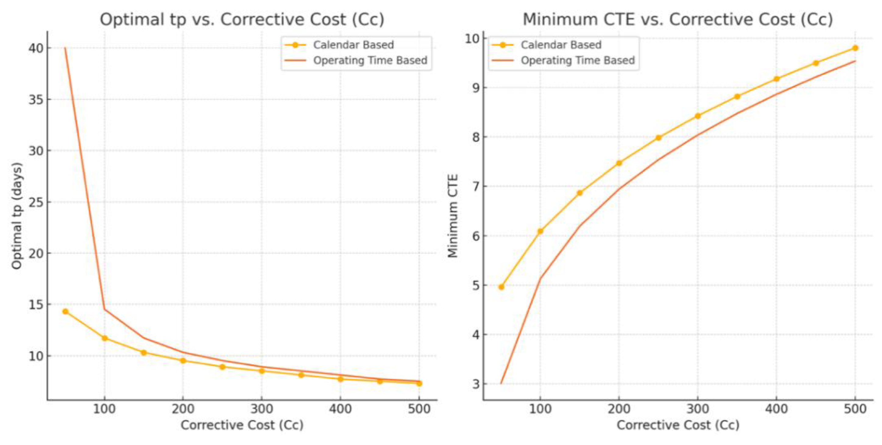
Is it possible now to have a graph showing the sensitivity of these optimal intervals with respect to variations in corrective cost from 50 to 500?

This is GPT-4o answer:

The graphs in Figure 6 provide insights into how the optimal maintenance intervals and costs respond to changes in the corrective maintenance cost.

The results in Figure 5 and Figure 6 leave us anything but indifferent. The possibility of optimizing the problem repeatedly under different conditions, obtaining the plot, visualizing the pattern of solution behavior with the effort invested, is simply brilliant.

6. Optimization using Partial Replacement Policies

A dialog to transfer the principles of this maintenance policy model is as follows:

• Prompt 6. Transferring principles of partial replacement policy.

We will now model partial replacement policies, these models are based in the idea that on many occasions a system fails does not need to be completely replaced (ST) to come back to normal operating conditions, only a partial preventive replacement (SPP) is needed. SPPs are overhauls after a certain time interval (with length Ti), setting the system to as an “as good as new” situation. After a certain number of overhauls, these will be more costly than a total system replacement. The subindex i measures the number of periods before the overhaul, with i=1 to k, with k-1 as maximum number of overhauls once total replacement (ST) will take place after period k. Once this is clear, we will study two possible partial replacement models existing in the literature:

• [1] Models with partial preventive replacements (preventive overhauls) and minimal repairs; and
• [2] Models with partial preventive replacements (preventive overhauls) and corrective interventions (corrective overhauls).

Let’s try to model partial replacement with minimal repairs first. We will consider that the total system replacement (ST) is after (k-1) partial preventive replacements (overhauls) SPPs. For a system with (i-1) overhauls, with i<k, each overhaul i takes place after Ti calendar time. In case of failure, a minimal repair is accomplished, not affecting the failure rate of the system (“as bad as old” after the minimal repair). After SPP and ST the systems is “as good as new”.

Regarding CTE formulation, please consider that:

$$CTE(k,T1,...Tk)=\left(\right(k-1)Cspp+Cst+Crm\sum N(Ti\left)\right)/\sum Ti,$$

with i=1...k. Where N(Ti) could depend on a λi(t), i.e., a failure rate resulting in minimum repairs that is different for each interval, i.e., it changes after each overhaul. I do not want code so far, but only the problem formulation.

The answer and feedback to this communication from GPT-4o is as follows:

Partial Replacement with Minimal Repairs. Conceptual Framework:

• We consider a system that undergoes partial preventive replacements (SPPs or overhauls) and minimal repairs.
• A total system replacement (ST) occurs after k−1 overhauls.
• Each overhaul ii takes place after Ti calendar time, with ii ranging from 1 to k−1.
• In case of failure within the i-th interval, a minimal repair is performed, returning the system to an “as bad as old” condition (i.e., the failure rate remains unchanged after the repair).
• After an SPP or ST, the system is restored to an “as good as new” condition.

Objective: Minimize the total expected maintenance cost CTE(k,T1,…,Tk).

Formulation:

$$CTE(k,T1,\dots ,Tk)=\left(\right(k-1)Cspp+Cst+Crm\sum _{i=1}^{k}N\left(Ti\right))/\sum _{i=1}^{k}Ti$$

where:

• k is the total number of intervals, including the interval after the last overhaul leading to the total replacement.
• Cspp is the cost of each partial preventive replacement (overhaul).
• Cst is the cost of total system replacement.
• Crm is the cost of minimal repairs.
• N(Ti) is the number of minimal repairs in the ii-th interval.
• Ti is the calendar time length of the i-th interval.
• Failure Rate and Minimal Repairs:
• Let λi(t) denote the failure rate of the system during the ii-th interval.
• N(Ti) is dependent on λi(t), which changes after each overhaul.

Steps to Solve the Problem:

• Define Failure Rate λi(t): Determine how λi(t) evolves within each interval Ti. This may involve fitting a failure rate model for each interval based on historical data or assumptions.
• Calculate N(Ti): Integrate the failure rate over each interval to find the expected number of minimal repairs:$N\left(Ti\right)={\int }_0^{Ti}\lambda i\left(t\right)\hspace{0.17em}dt$Formulate CTE Expression: Substitute the values of N(Ti) and the corresponding costs into the $CTE$ expression to obtain the expected total maintenance cost.
• Optimize T1, …,Tk: Optimize the intervals $\mathrm{T}\mathrm{i}$ to minimize the total expected maintenance cost CTE(k, T1, …, Tk).

Other Important Considerations:

• Cost Parameters: Ensure accurate estimation of Cspp, Cst, and Crm.
• Failure Rate Modeling: Accurate modeling of λi(t) for each interval is crucial for precise calculation of N(Ti).
• Optimization Method: Choose an appropriate optimization method (e.g., gradient descent, genetic algorithms) to minimize CTE(k, T1, …, Tk).

This formulation provides a comprehensive framework for analyzing and optimizing the maintenance strategy involving partial preventive replacements and minimal repairs.

• Prompt 7. Outputs of the first partial replacement policy cost calculation

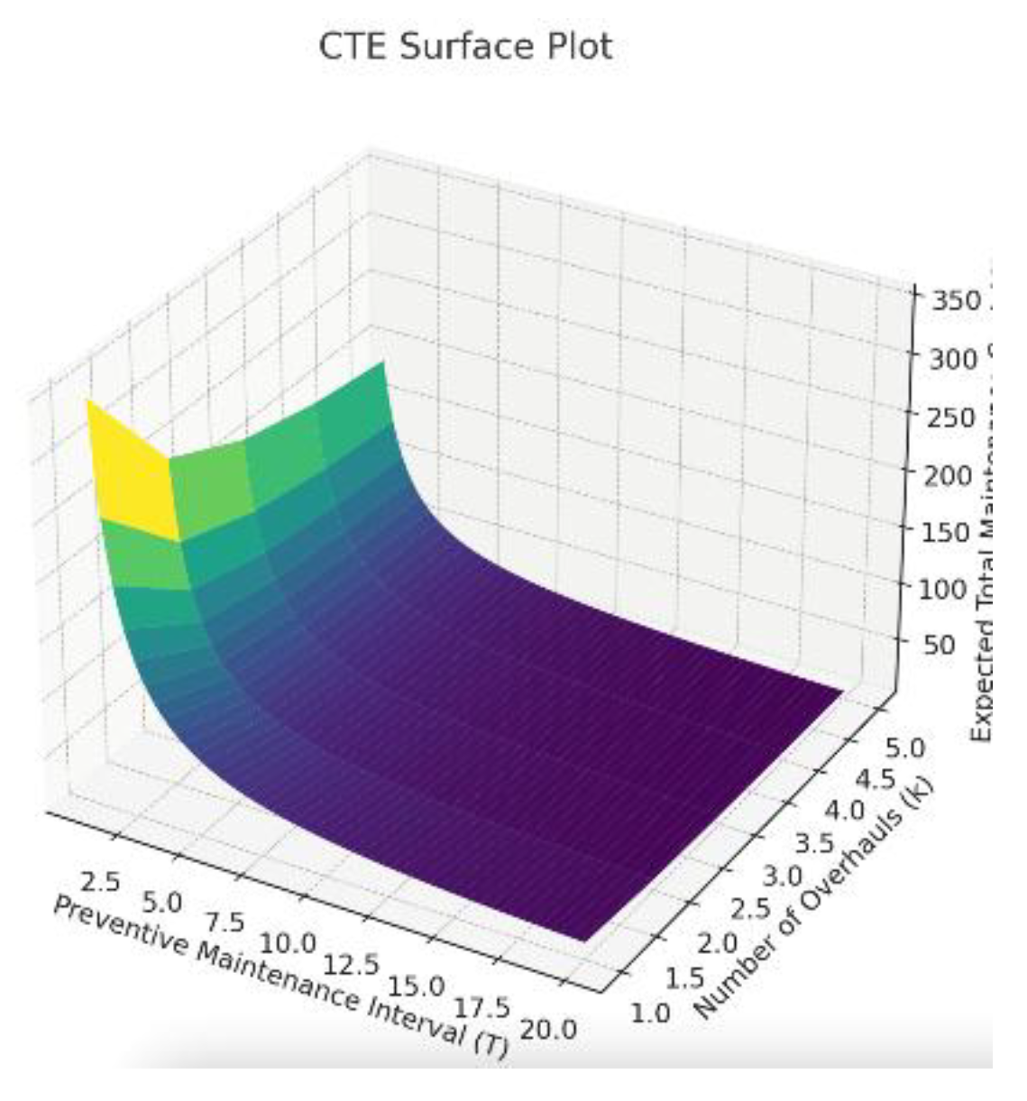
Can we make a plot of CTE as a surface to see its result when T and K change? I would like to make the plot thinking with a maximum number of K equal to 5 and T=20, to identify the minimum.

Figure 7. Partial replacement (with preventive overhaul + minimal repairs) policy cost output as per Prompt 7.

Figure 7. Partial replacement (with preventive overhaul + minimal repairs) policy cost output as per Prompt 7.

The answer of GPT-4o is:

• Prompt 8. Transferring principles of the second partial replacement policy.

Let’s now model 2) Partial preventive replacements (preventive overhauls) and corrective interventions (corrective overhauls). OK? to do so, let’s consider that the complete system has a probability to have a failure requiring a complete corrective overhaul (IC), this IC will cost more than a normal overhaul (Cic=Cspp+Ceic, with Ceic the extra cost compared to the overhaul cost). The probability will also be a Weibull function but much less probable than a minimal repair (please guess a weibull). And then what happens is that if we have an IC, we overhaul, and the system is as good as new afterwards. Now we will to preventive overhauls only if we do not have a IC before T. Now without minimal repairs

$$CTE(k,T1,...Tk)=\left(\right(k-1)Cspp+Cst+Ceic\sum Fi(Ti\left)\right)/\sum \left(Ti\mathrm{*}Ri\right(Ti)+Mi(Ti\left)\right),$$

could you formulate the problem?

This is the GPT-4o answer:

Problem Formulation. Scenario Description

• Preventive Overhauls (SPP): These are scheduled preventive replacements that occur after a certain time interval Ti. After each preventive overhaul, the system is considered “as good as new.”
• Corrective Overhauls (IC): These occur when a failure happens that necessitates a complete overhaul before the next scheduled preventive overhaul. The cost of an IC includes the cost of a preventive overhaul plus an additional cost, represented as Cic = Cspp + Ceic After an IC, the system is also considered “as good as new.”

Failure Probabilities and Costs

• The probability of requiring a corrective overhaul (IC) is modeled by a Weibull distribution with parameters βic and ηic. This distribution will have a lower failure rate compared to minimal repairs.
• The cost of each corrective overhaul (IC) is Cic, which includes the standard overhaul cost CsppCspp and an additional cost Ceic.

Key Functions

• Reliability Function (Survival Probability) $Ri\left(t\right)$: This indicates the probability that the system does not fail by time tt in the i-th interval.
• Probability of Corrective Overhaul $Fi\left(t\right)$: The probability that a corrective overhaul is needed by time t in the i-th interval.
• Integral of Time-Weighted Density$Mi\left(t\right)$: This represents the expected value of time until failure for each interval.

Cost Function (CTE) Calculation

$$CTE(k,T1,\dots ,Tk)=(\left(k-1\right)Cspp+Cst+Ceic\bullet \sum Fi\left(Ti\right))/\sum (Ti\bullet Ri(Ti)+Mi(Ti\left)\right)$$

Components:

• $(k-1)Cspp$: Total cost of k−1 preventive overhauls.
• $Cst$: Cost of the final total system replacement after the last preventive overhaul.
• $Ceic\bullet \sum Fi\left(Ti\right)$: Total additional cost due to corrective overhauls.
• $Ti\bullet Ri\left(Ti\right)$: Expected time without failure for the i-th interval.
• $Mi\left(Ti\right)$: Expected time to failure weighted by the density function for the ii-th interval.

7. AI Designed Model of Hybrid Policies Optimization

The integration of generative AI, specifically GPT, in developing maintenance models has unlocked new ways to approach complex maintenance policy combinations. In this section, we examine a model generated by GPT that combines two distinct partial replacement policies: one incorporating minimal repairs, where repairs maintain the current degradation level, and another with corrective interventions, where replacements restore the system to an optimal state. Through pre-trained learning, GPT has identified a method to unify these approaches, creating a hybrid model that reflects real-world scenarios where both minimal repairs and corrective interventions are often necessary within the same maintenance framework. This new model not only highlights the adaptability of GPT in merging and modifying maintenance policies but also demonstrates the power of generative AI to dynamically construct sophisticated solutions based on prior knowledge. By building on existing policies and customizing their application to meet varied operational requirements, GPT facilitates the design of versatile maintenance strategies. This combined approach provides a more holistic and flexible framework for maintenance optimization, reflecting the complexity of industrial needs while enhancing the strategic value of AI-driven insights in maintenance management.

• Prompt 9. Designing the prompt to combine models

What prompt do I have to do to get these two policies combined?

This is GPT-4o answer:

I want to combine two maintenance policies: minimum repairs and preventive replacements (SPP) with corrective interventions (CI). Here are the details:

• Preventive Overhauls (SPP): These are scheduled overhauls that are performed after a certain interval of time. Ti, leaving the system “as new”. Costo f each SPP is Cspp.
• Corrective Overhauls (CI): These are unscheduled interventions due to serious failures that require a complete repair before the next scheduled SPP. Costo f an IC is Cic=Cspp+Ceic , with Ceic named additional cost. The probability of the occurrence of a CI is modeled by a Weibull distribution with parameters βic and ηic.
• Minimal Repairs: These repairs occur when minor failures occur, returning the system to an “as bad as before” state without altering the failure rate. The cost of each minimal repair is Crm. The number of minimal repairs is N(Ti) is determined by integrating the failure rate over the interval adjusted by the expected duration.

Goal: I want to calculate the total expected cost (CTE) that considers both policies, including SPPs, CIs and minimum repairs. The CTE calculation should consider the following variables:

• The reliability function for IC Ric(t), which represents the probability that a corrective intervention does not occur until time t.
• The cumulative probability of failure for IC Fic(t), which is the probability that a corrective intervention occurs in the interval.
• The time-weighted density integral for CI Mi(Ti), based on the probability density of CIs.
• The number of minimum repairs N(Ti), which considers the expected duration of the interval, calculated as TiRic(Ti)+Mi(Ti).

I want you to explain to me how the total expected cost (TEC) is formulated in this context, including all the above components, and how they should be combined to obtain the final TEC expression. It is important that the calculation correctly reflects the coexistence of minimum repairs and corrective interventions, considering the respective Weibull distributions and associated costs.

• Prompt 10. Validating hybrid model formulation corrections

Give me your formulation corrections

This is the GPT-4o answer:

Formulation Corrections for the combined problem

• Reliability Function for CI Ric(t): represents the probability that a corrective intervention does not occur until time t.
• Time-weighted density integral for IC Mi(Ti): Based on the probability density function for corrective interventions fic(t): $Mi\left(Ti\right)={\int }_0^{Ti}tfic\left(t\right)dt$Number of Minimum Repairs Ni(Ti): Calculated using Rrm (Ti) instead of Ric(Ti) and the expected duration of the interval, considering that minimum repairs can occur before a corrective intervention (CI) is performed: $Ni\left(Ti\right)={\int }_0^{TiRic\left(Ti\right)+Mi\left(Ti\right)}\lambda rm\left(t\right)dt$. Where λrm(t) is the failure rate of the minimum repairs.
• Expected Total Cost (CTE):

  $$CTE(k,T1,...,Tk)=\left(\right(k-1)Cspp+Cst+Cic\sum Fic(Ti)+Crm\sum Ni(Ti\left)\right)/\sum \left(TiRic\right(Ti)+Mi(Ti\left)\right)$$

This adjusted model more accurately reflects the dynamics of system failures, considering both minimum repairs and corrective interventions, with their respective Weibull distributions and associated costs. This distinction is essential to adequately model the system behavior and plan the system’s performance.

8. AI Designed Discrete Event Simulation Model for Finite Time Period Analysis of the Previous Problem

Using generative AI to develop simulation models for finite-time analysis offers several key advantages. First, generative AI can quickly adapt and generate models that reflect real-world conditions over a specific period, capturing the nuances of asset wear and failure rates without the need for manual reprogramming. This adaptability allows decision-makers to focus on specific operational windows and simulate the effects of different maintenance strategies within those periods. Moreover, once a generative AI-driven model is created, it can easily integrate with Monte Carlo simulations to explore various probabilistic outcomes, helping to assess the uncertainty and risk associated with different maintenance scenarios. The use of Monte Carlo simulations provides a robust framework for understanding the impact of random events, optimizing the maintenance schedule by running thousands of simulations and determining the most cost-effective and reliable strategy. This combination of generative AI with Monte Carlo simulations leads to a highly flexible and powerful approach for analyzing and optimizing maintenance policies in real-world industrial settings.

• Prompt 11. Simulating the finite time problem for potential optimization

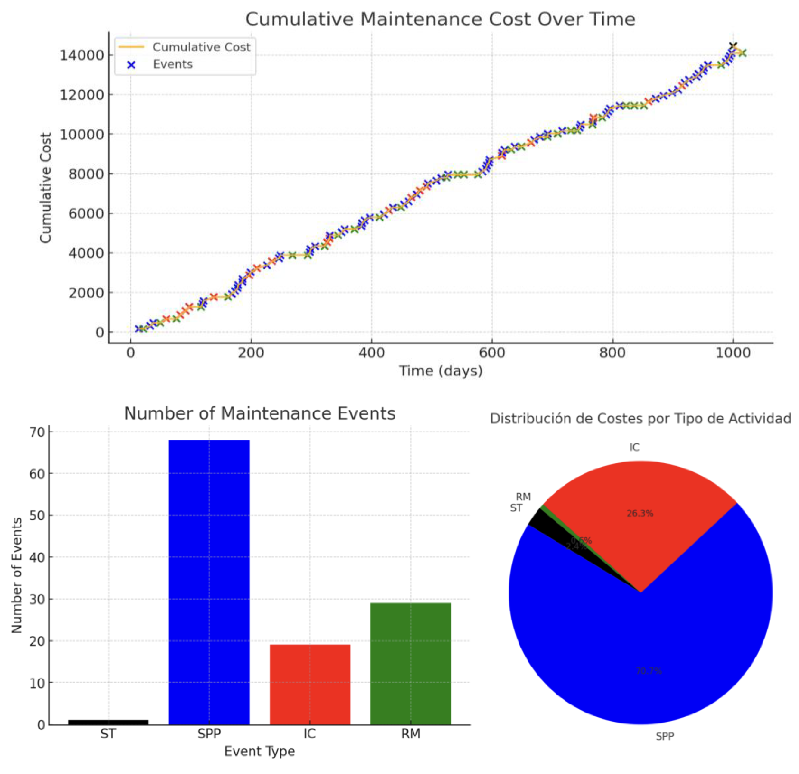
Is it possible to simulate for a certain finite period these maintenance policies and see the cost results generated? numbers of STs, SPPs, ICs, RMs, etc, and the costs for each activity we have incurred?

This is GPT-4o answer:

Code Explanation is as follows:

Failure Time Generation: Random times for RM and IC failures are generated based on their respective Weibull distributions. A random time is generated for the next SPP.

Event Determination: It is determined which event occurs first (RM, IC or SPP) and the accumulated counters and costs are updated.

Event Logging: Each event is logged along with its time of occurrence and cost.

Visualization: Cumulative cost graph over time, Bar chart of the number of events by type.

This basic example can be expanded and adjusted according to specific needs, including consideration of different maintenance periods, different repair policies, and detailed cost analysis.

Figure 8. Sample output of the finite time problem simulation in Prompt 11.

Figure 8. Sample output of the finite time problem simulation in Prompt 11.

9. The AI Generated Code per Case Study: Considerations

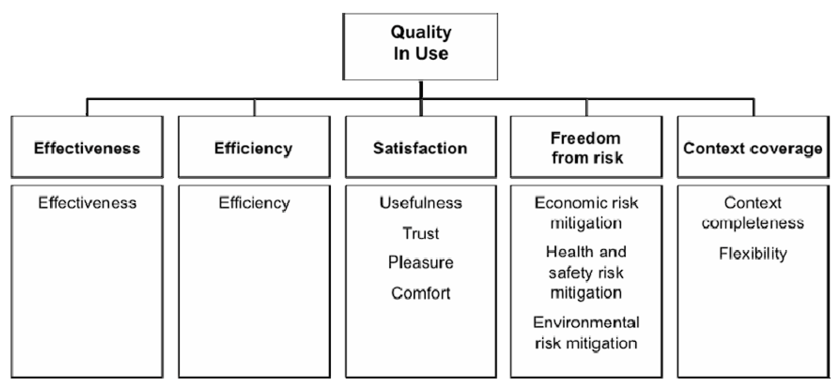
The paper focuses on the use of ChatGPT as an assistant for the development and analysis of maintenance models. As a software, it is relevant to perform a quality analysis of the interaction with it and its capabilities. A critical approach is required to ensure that the defined models are valid, up-to date and applicable in the different contexts that may arise.

With this in mind, we have dipped into the ISO 25000 series (SQuaRE – System and Software Quality Requirements and Evaluation), specifically into the 25010 series (Quality Model Division). ISO 25010 proposes the following criteria to be analyzed to evaluate a code, concerning the possible outcomes resulting from the interaction with it, within its “Quality in Use” model ? See Figure 9 and some examples of application in [18] or [22]—:

• Effectiveness: accuracy and completeness with which users achieve specified goals.
• Efficiency: resources expended in relation to the accuracy and completeness with which users achieve goals.
• Satisfaction: degree to which user needs are satisfied when a product or system is used in a specified context of use.
• Freedom from risk: degree to which a product or system mitigates the potential risk to economic status, human life, health, or the environment.
• Context coverage: degree to which a product or system can be used with effectiveness, efficiency, freedom from risk and satisfaction in both specified contexts of use and in contexts beyond those initially explicitly identified.

Figure 9. SQuaRE “Quality in Use” evaluation criteria.

Figure 9. SQuaRE “Quality in Use” evaluation criteria.

9.1. Quality in Use assessment

• Effectiveness: Concerning goal’s satisfaction, the chatbot is proven useful when it comes to assessing simple tasks. It has to be noted that the model might usually behave in a narrow-minded way. For example, when defining functions, parameters such as alpha or costs won’t be included as function inputs, but as simple constants, unless explicitly told to do so.

When it comes to more complex tasks, the model may start to provide wrong answers. One example is Prompt 11; when asked to develop a fairly simple simulation model, several attempts are necessary until a decent solution is achieved – the main failures in this case were wrong logical rules when inputting costs, a misunderstanding of concepts clearly stated when deterministic parameters such as scheduled preventive maintenance time intervals was randomized, and a not-so-reliable method for generating random time intervals. Similarly, when performing stochastic simulation, the chatbot does not consider the necessity of statistical analysis to obtain reliable results, unless explicitly told to.

• Efficiency: The time consumption of the Chatbot’s processing is negligible. However, there are some further issues that need to be addressed when it comes to resource consumption. First of all, it is important to consider that many companies will not be able to/want to upload sensitive data to an external cloud-based data system such as OpenAI’s ChatGPT platform. Running extensive AI models might require high-end hardware, posing an elevated cost that might not be so efficient if this is the only task it will be used for. Also, it is necessary to provide very specific and detailed instructions, and colloquial speech should be avoided at any costs – this usually leads to the need of thoroughly review the written prompts. If personnel with decent programming skills is available, the same task could be achieved as fast as with the Chatbot but avoiding any extensive hardware requirements and the use of the AI itself, as the task is fairly simple.
• Satisfaction. Personal user satisfaction has been evaluated from two different Points of View: A skilled programmer perspective and a non-skilled programming one.

On the one hand, for a person with little knowledge of programming, the use of the chatbot is highly satisfactory, as it leverages programming tools overtaking the lack of knowledge.

On the other, a person with enough programming knowledge to develop these models in Python might find uncomfortable the use of the chatbot because of several reasons: these are for example the necessity of explicitly mentioning rather trivial things, such as the inclusion of parameters as inputs rather than as constants of functions.

It is very important to consider the trust implications. Users may trust or distrust the chatbot because of very different reasons. If a person with enough programming knowledge considers the source code provided simple or notices flaws, might feel discouraged to continue using the tool. However, the chatbot can be asked to provide the mathematical formulation being used, so it can be checked and improve users trust when simply prompting the chatbot to develop models (not source codes). Nevertheless, this option is not always suitable (a simulation model might not be as simple to be mathematically formulated and revised)

• Freedom from risk: As stated before, the chatbot might sometimes commit errors that can only be checked by looking at the source code that the chatbot generated and used to accomplish the task. This means that a user unexperienced in coding might consider as valid wrong solutions, posing a potential risk. This also leads to an ironical situation where a programmer might be requested to check the source code and carry out necessary corrections but could have been tasked before to develop the model from scratch, being this potentially more efficient.
• Context coverage: Chatbots like ChatGPT allow the user to interact using different languages – this entails that language barriers might be easily surpassed when the user’s mother tongue is supported. Also, it is possible to generate models dynamically and updating input data through interaction with the chatbot. However, it is proven that at certain cases the chatbot might give wrong answers, leading to potential risks. Also, the nuances defining the barrier between a good or a bad answer might be unclear, therefore the context coverage might be considered as unclear, or null in the worst case, based on the inability of potential users to judge correctness of answers.

10. Conclusions Regarding the Use of AI For Modelling Policies

The use of generative AI like GPT for generating and optimizing maintenance policies offers several advantages. First, GPT can dynamically create tailored maintenance strategies that adjust to varying scenarios, combining different policy types such as minimal repairs, preventive overhauls, and corrective interventions. This flexibility allows for hybrid strategies that better reflect the complexity of real-world maintenance needs. Additionally, GPT can autonomously re-formulate models based on operational changes, ensuring that maintenance policies remain up-to-date and optimized. Another key advantage is the ability to analyze policies over finite periods and explore probabilistic outcomes using Monte Carlo simulations, which can improve decision-making by offering insight into potential risks and costs. AI-driven models also provide improved visualizations and interaction, allowing users to simulate, visualize, and adjust strategies as needed. Ultimately, this results in better cost optimization, risk mitigation, and the ability to implement data-driven maintenance decisions more efficiently.

On the other hand, several challenges exist when applying GPT in this context. One key limitation is that the quality of AI-generated models depends heavily on the availability and accuracy of training data. If the data is incomplete or biased, it may lead to unreliable or overly simplified policies. Additionally, complex real-world scenarios may require more sophisticated modeling, which AI systems may oversimplify or fail to account for. While AI models are flexible, they can also be computationally expensive to run, especially when combined with techniques like Monte Carlo simulations. Furthermore, the interpretability of GPT-generated models may pose a challenge for domain experts, as the reasoning behind the AI’s decisions might be difficult to trace. Finally, there’s a risk of overfitting to specific scenarios, making the models less effective in broader applications. Despite these challenges, the potential benefits of using generative AI in maintenance policy development make it a powerful tool for industrial optimization.

Table 1. Advantages and disadvantages found when using AI for modelling maintenance policies.

Advantages	Disadvantages
− Dynamic Model Generation: GPT adapts to various scenarios.	− Data Dependency: Results depend on the quality of training data.
− Combination of Maintenance Policies into hybrid strategies.	− Complexity of Real-World Scenarios: Models may miss key nuances.
− Improved Decision Support through simulations and visualizations.	− Computational Cost: High cost for generating and updating models.
− Automation of Model Re-formulation based on changing conditions.	− Interpretability: AI models may be difficult to interpret.
− Handles Finite Time and Real-Time Problem Solving.	− Risk of Overfitting: Models may be too specific for general use.
− Cost Optimization and Risk Mitigation.	− Lack of Physical Constraints: Generated models may be impractical.
− Provides Visualization and Interaction for better decision-making.	− Dependence on Human Input for final decisions and validation.

Table 1. Advantages and disadvantages found when using AI for modelling maintenance policies.

Advantages	Disadvantages
− Dynamic Model Generation: GPT adapts to various scenarios.	− Data Dependency: Results depend on the quality of training data.
− Combination of Maintenance Policies into hybrid strategies.	− Complexity of Real-World Scenarios: Models may miss key nuances.
− Improved Decision Support through simulations and visualizations.	− Computational Cost: High cost for generating and updating models.
− Automation of Model Re-formulation based on changing conditions.	− Interpretability: AI models may be difficult to interpret.
− Handles Finite Time and Real-Time Problem Solving.	− Risk of Overfitting: Models may be too specific for general use.
− Cost Optimization and Risk Mitigation.	− Lack of Physical Constraints: Generated models may be impractical.
− Provides Visualization and Interaction for better decision-making.	− Dependence on Human Input for final decisions and validation.

11. Conclusions Regarding the Code Generated

The overall findings indicate that ChatGPT’s code generation capabilities can be highly beneficial for relatively simple programming tasks, especially for users with limited technical knowledge. In such cases, the tool allows for rapid development of basic models or prototypes, thereby reducing the initial effort needed to begin coding. However, when confronted with more complex or specialized tasks, ChatGPT often omits crucial parameters or treats them inappropriately, for instance by fixing them as constants rather than incorporating them as variables. It also tends to produce logical inconsistencies, particularly in cost modeling, scheduled maintenance intervals, and stochastic simulations, where it does not account for the necessary statistical analysis unless prompted explicitly.

From the perspective of “Quality in Use” as articulated by ISO 25010, ChatGPT is effective at providing guidance for solution development but requires meticulous prompt specification to ensure completeness and accuracy. Insufficiently detailed prompts can result in code that is incomplete or erroneous, posing risks for non-expert users. While the efficiency of ChatGPT in terms of response time is high, concerns remain regarding the management of sensitive data on external servers and the potential costs of implementing on-premise hardware solutions. User satisfaction, moreover, depends heavily on programming expertise. Novices may find it highly satisfactory, as ChatGPT delivers functional code quickly, whereas experienced programmers may find the need to explicitly spell out trivial details and verify or correct the resulting code burdensome.

Despite the broad applicability of ChatGPT across different contexts and languages, its reliability varies, particularly when users are not equipped to detect potential errors. This variability increases the risk of integrating unverified code in critical environments. As a result, any code produced by ChatGPT should be perceived as an initial draft rather than a definitive solution. Review and, if necessary, refinement by domain experts or skilled programmers are essential to ensure that the final implementation is robust and aligns with the intended purpose.

In sum, ChatGPT offers valuable support for rapid prototyping and instructional activities. However, its limitations underscore the importance of active expert oversight, rigorous validation of generated outputs, and careful consideration of the context in which the code will be deployed. This balanced approach preserves the tool’s advantages while minimizing the risks associated with incomplete or erroneous solutions.

Table 2. Summary of pros and cons found in the quality of ChatGPT code generation.

Pros	Cons
− Rapid Development of Basic Models or Prototypes	− Omission of Crucial Parameters
− Ease of Use for Non-Experts	− Logical Inconsistencies
− Efficiency in Response Time	− Dependency on Prompt Specificity
− Applicability Across Contexts and Languages	− Incomplete or Erroneous Code
− Instructional Support	− Reliability Concerns
− User Satisfaction for Novices	− Burden for Experts
− Cost-Effective for Prototyping	− Security Risks
− Drafting Support	− Requires Expert Oversight

Table 2. Summary of pros and cons found in the quality of ChatGPT code generation.

Pros	Cons
− Rapid Development of Basic Models or Prototypes	− Omission of Crucial Parameters
− Ease of Use for Non-Experts	− Logical Inconsistencies
− Efficiency in Response Time	− Dependency on Prompt Specificity
− Applicability Across Contexts and Languages	− Incomplete or Erroneous Code
− Instructional Support	− Reliability Concerns
− User Satisfaction for Novices	− Burden for Experts
− Cost-Effective for Prototyping	− Security Risks
− Drafting Support	− Requires Expert Oversight

References

- Anders, G. J., & Sugier, J. (2006). Risk assessment tool for maintenance selection. Proceedings of International Conference on Dependability of Computer Systems, DepCoS-RELCOMEX 2006. [CrossRef]
- Barlow, R., & Hunter, L. (1960). Optimum Preventive Maintenance Policies. Operations Research, 8(1). [CrossRef]
- Ćelić, J., Bronzin, T., Horvat, M., Jović, A., Stipić, A., Prole, B., Maričević, M., Pavlović, I., Pap, K., Mikota, M., & Jelača, N. (2024). Generative AI in E-maintenance: Myth or Reality? International Journal of Advanced Computer Science and Applications, 15(2), 45-52.
- Chang, C. C. (2014). Optimum preventive maintenance policies for systems subject to random working times, replacement, and minimal repair. Computers and Industrial Engineering, 67(1). [CrossRef]
- Chareonsuk, C., Nagarur, N., & Tabucanon, M. T. (1997). A multicriteria approach to the selection of preventive maintenance intervals. International Journal of Production Economics, 49(1). [CrossRef]
- Cho, D. I., & Parlar, M. (1991). A survey of maintenance models for multi-unit systems A Survey of Preventive Maintenance Models for Stochastically Deteriorating Single-Unit Systems, by. European Journal of Operational Research, 51(1). [CrossRef]
- Coster, M., & Liu, Q. (2015). An Imperfect Preventive Maintenance Policy Considering Reliability Limit. Journal of Engineering Research and Applications, 5(2).
- Ding, S. H., & Kamaruddin, S. (2015). Maintenance policy optimization—literature review and directions. International Journal of Advanced Manufacturing Technology, Vol. 76. [CrossRef]
- Haridasan, P. K., & Kumar, V. (2024). Generative AI in Manufacturing: A Review of Innovations, Challenges, and Future Prospects. Journal of Artificial Intelligence and Machine Learning, 2(2), 1-15.
- Jafari, L., Naderkhani, F., & Makis, V. (2018). Joint optimization of maintenance policy and inspection interval for a multi-unit series system using proportional hazards model. Journal of the Operational Research Society, 69(1). [CrossRef]
- Journal, E., Pham, H., & Wang, H. (1996). EUROPEAN JOURNAL OF OPERATIONAL RESEARCH Imperfect maintenance. In Operational Research (Vol. 94).
- Laggoune, R., Chateauneuf, A., & Aissani, D. (2009). Opportunistic policy for optimal preventive maintenance of a multi-component system in continuous operating units. Computers and Chemical Engineering, 33(9). [CrossRef]
- Marais, K. B., & Saleh, J. H. (2009). System value trajectories, maintenance, and its present value. Safety, Reliability and Risk Analysis: Theory, Methods and Applications - Proceedings of the Joint ESREL and SRA-Europe Conference, 1. [CrossRef]
- Mohapatra, A. (2024). Generative AI for Predictive Maintenance: Predicting Equipment Failures and Optimizing Maintenance Schedules Using AI. International Journal of Scientific Research and Management (IJSRM), 12(11), 1648-1672.
- Nakagawa, T. (1979). Optimum policies when preventive maintenance is imperfect. IEEE Transactions on Reliability, R-28(4). [CrossRef]
- Nguyen, D. G., & Murthy, D. N. P. (1981). OPTIMAL PREVENTIVE MAINTENANCE POLICIES FOR REPAIRABLE SYSTEMS. Operations Research, 29(6). [CrossRef]
- OpenAI. (2024). Hello GPT-4o. Retrieved from https://openai.com/index/hello-gpt-4o/.
- Pereira, D. S., Bezerra, L. F. V., Nunes, J. S., Barroca Filho, I. M., & Lopes, F. A. S. (2023). Performance Efficiency Evaluation based on ISO/IEC 25010:2011 applied to a Case Study on Load Balance and Resilient. [CrossRef]
- Pereira, F. H., Melani, A. H. de A., Kashiwagi, F. N., Rosa, T. G. da, Santos, U. S. dos, & Souza, G. F. M. de. (2023). Imperfect Preventive Maintenance Optimization with Variable Age Reduction Factor and Independent Intervention Level. Applied Sciences (Switzerland), 13(18). [CrossRef]
- Pérez, F., & Granger, B. E. (2007). IPython: A System for Interactive Scientific Computing. Computing in Science & Engineering, 9(3), 21–29. [CrossRef]
- Pierskalla, W. P., & Voelker, J. A. (1976). A survey of maintenance models: The control and surveillance of deteriorating systems. Naval Research Logistics Quarterly, 23(3). [CrossRef]
- Prabowo, W. A. (2024). Developing Compliant Audit Information System for Information Security Index: A Study on Enhancing Institutional and Organizational Audits Using Web-based Technology and ISO 25010:2011 Total Quality of Use Evaluation. International Journal on Informatics Visualization, 8(1). [CrossRef]
- Samrout, M., Châtelet, E., Kouta, R., & Chebbo, N. (2009). Optimization of maintenance policy using the proportional hazard model. Reliability Engineering and System Safety, 94(1). [CrossRef]
- Santos, A. C. de J., Cavalcante, C. A. V., & Wu, S. (2023). Maintenance policies and models: A bibliometric and literature review of strategies for reuse and remanufacturing. Reliability Engineering and System Safety, Vol. 231. [CrossRef]
- Shafiee, M., & Finkelstein, M. (2015). An optimal age-based group maintenance policy for multi-unit degrading systems. Reliability Engineering and System Safety, 134. [CrossRef]
- Sharma, A., Yadava, G. S., & Deshmukh, S. G. (2011). A literature review and future perspectives on maintenance optimization. Journal of Quality in Maintenance Engineering, Vol. 17. [CrossRef]
- Tian, Z., & Liao, H. (2011). Condition based maintenance optimization for multi-component systems using proportional hazards model. Reliability Engineering and System Safety, 96(5). [CrossRef]
- Valdez-Flores, C., & Feldman, R. M. (1989). A survey of preventive maintenance models for stochastically deteriorating single-unit systems. Naval Research Logistics (NRL). [CrossRef]
- Wakiru, J., Pintelon, L., Muchiri, P. N., Chemweno, P. K., & Mburu, S. (2020). Towards an innovative lubricant condition monitoring strategy for maintenance of ageing multi-unit systems. Reliability Engineering and System Safety, 204. [CrossRef]
- Wang, H., & Pham, H. (1996). Optimal maintenance policies for several imperfect repair models. International Journal of Systems Science, 27(6). [CrossRef]
- Xu, Q. Z., Guo, L. M., Wang, N., & Fei, R. (2015). Recent advances in selective maintenance from 1998 to 2014. Journal of Donghua University (English Edition), 32(6).