
Submitted:
04 February 2025
Posted:
05 February 2025
You are already at the latest version
Abstract
This study has investigated the effectiveness of the large-eddy simulation version of the Weather Research and Forecasting Model (WRF-LES) in reproducing atmospheric conditions observed during the Perdigão field experiment. When comparing the results of the WRF-LES model with the observations, using LES settings can accurately repre-sent both large-scale events and the specific characteristics of atmospheric circulation at a small scale. Six sensitivity experiments are performed to evaluate the impact of different Planetary Boundary Layer (PBL) schemes, including the MYNN, YSU and Shin and Hong (SH) PBL models, as well as Large Eddy Simulation (LES) with Sma-gorinsky (SMAG), a 1.5-order turbulence kinetic energy closure model (TKE) and non-linear backscatter and anisotropy (NBA) subgrid-scale (SGS) stress models. Two case studies are selected to be representative of flow conditions. In the northeastern flow, the MYNN NBA simulation yielded the best result at a height of 100 m with an error rate of -0.03 m/s, although SH generally produces better results than PBL schemes. In the southwestern flow, MYNN 1.5 TKE simulation at station Mast 29 is the best result, with an error rate of -0.01 m/s. The choice of SGS models over complex terrain affects wind field features in the boundary layer more than above the boundary layer. The NBA model generally performed better results in complex terrain when compared to other SGS models. In general, the WRF-LES can model the observed flow with high-resolution topographic maps in complex terrain with different SGS models for both flow regimes.
Keywords:
Wind Energy
; Resource Assessment
; large eddy simulation
; planetary boundary layer
1. Introduction
Wind farm siting in complex terrain conditions creates significant challenges and requires thorough validation of modeling methods. The meso-micro coupling is one of the most widely used techniques nowadays. The higher horizontal resolution enables the accurate modeling of the boundary layer, resulting in a more accurate depiction of the temporal and spatial distribution of the atmosphere, boundary layer and turbulence [1,2,3,4,5,6,7,8,9,10].
The motion of winds in complex terrain is affected by the characteristics of the surface features (land class/roughness length) and the specific elevation of the area, including hills, ridges, and mountains [11]. Modeling wind farms in complex terrain requires a more sophisticated approach than the typically employed linearized models like WAsP [12]. Computational fluid dynamics (CFD) methods are being used more and more to predict flows over complex terrain areas to consider these phenomena and offer more precise predictions of wind resources [13]. However, enhancing numerical modelling techniques for complex terrain necessitates considering several microscale processes, such as flow recirculation and the impact of the topography. Atmospheric models like the Weather Research and Forecasting Model (WRF) allow for downscaling through grid nesting [14]. This means that the lateral boundary conditions for a smaller region in the model are determined by the outer grid simulations surrounding it.
To perform an accurate simulation of the turbulent flow field in the atmospheric boundary layer, it is required to conduct high-resolution simulations and account for the consequences of the large-scale features of the flow. A successful approach involves employing coupled mesoscale and microscale simulations, which accurately address different scales of atmospheric motion. The turbulence effects in traditional mesoscale grid cells, which have large horizontal footprints (with a horizontal grid spacing of approximately a couple of thousands m), are parameterized only in the vertical direction. This is done using turbulence schemes such as the Mellor-Yamada-Nakanishi-Niino level 2.5 (MYNN) scheme and the Yonsei University (YSU) scheme [15,16]. The assumption of horizontal homogeneity is made by these schemes. On the other hand, when conducting turbulence-resolving simulations with a horizontal grid spacing of 100 m, turbulence models are required to parameterize the turbulence in all three orthogonal directions, such as the Smagorinsky approach or the Lilly method down to the inertial subrange scales [17,18,19].
Large Eddy Simulation (LES) is a method that involves resolving the energy-producing scales of three-dimensional atmospheric turbulence, while filtering out the smaller-scale component of the turbulence spectrum from the flow field using a spatial filter [20,21]. By choosing a filter scale within the inertial subrange, the flow field might be divided into two parts: a resolved component that includes many scales responsible for turbulent transport and turbulence kinetic energy production, and a subfilter component that consists of scales within the turbulence cascade [22,23]. The subfilter component’s main role is to dissipate energy from the resolved scales. The effects of the unresolved scales are captured within the subfilter-scale (SFS) stress. SFS stresses and fluxes are typically represented using SGS models, which offer time and space-dependent inputs for the explicitly resolved turbulent motion. These models ain to accurately replicate the statistical dissipation of energy in the turbulance cascade. The SGS can have a significant impact on the performance of LES. Additional information regarding the incorporation of Large Eddy Simulation into the Weather Research and Forecasting model can be found in the works of Mirocha and Kirkil [24,25].
Over the past few decades, researchers have created and refined large eddy simulation models that effectively simulate turbulence in the atmospheric boundary layer. These models also account for the interaction between the atmosphere and the ground surface, as well as the formation of the boundary layer [26,27,28,29,30,31,32].
In addition, LES simulations conducted in the WRF Model can utilize a wide range of atmospheric physics parameterizations, including a developing collection of parameterizations that are sensitive to scale [33,34]. Although LES is ideal for studying turbulent flow in the atmosphere at the scale of the Weather Research and Forecasting model, the model’s use of terrain-following coordinates makes it challenge operate LES over more complex or steep terrain [35,36]. Terrain-following coordinates are effective for mesoscale simulation resolutions. However, when high resolutions are utilized to record steep terrain slopes, numerical errors can occur, leading to a grid that is extremely skewed and has significant numerical inaccuracies [37,38,39,40,41].
Field observations are necessary to validate numerical models for complex terrain. One of the first field studies at Askervein hill is investigated an isolated hill [42]. The Bolund hill campaign was another campaign that was carried out over an isolated hill in Denmark, outlined by Bechmann [43]. Rodrigo conducted the Alaiz field campaign in Spain, which encompassed mountain valley topography [44]. Perdigão field campaign is the selected test site for this study conducted in Portugal in 2017 [45]. The Perdigão experiment completed a comprehensive analysis of the airflow along two parallel ridges and yielded significant data for the characterization of flow in complex terrain [9,10,46,47,48,49].
Ensuring suitable treatment of the planetary boundary layer (PBL) in the “gray zone” is another crucial concern in multiscale simulations on complex terrain, in addition to the correct parameterization of turbulence. Within the resolution range of around 1.5 km to 100 m, known as the ’gray zone’ or ’terra incognita’, models begin to explicitly resolve the bigger turbulent eddies [50,51,52,53,54,55]. Implementing a turbulence scheme may thus deteriorate the depiction of the bigger eddies, while still being essential to parameterize the smaller components of the turbulent spectrum [50,53,56,57].
Mesoscale turbulence parameterization are not appropriate for the gray zone scales and too large for an LES scheme to accurately represent turbulent eddies. When dealing with complex terrain, a substantial increase in the mesh refinement ratio might result in a notable discrepancy in topography at the boundaries between the mesoscale and the nested LES domains. Hence, it is crucial to examine the model’s performance at gray zone sizes in areas with complex topography.
The aim of this study is to facilitate the shift towards high-resolution atmospheric modeling by assessing the advantages and drawbacks of existing approaches. The WRF-LES model was tested for the accuracy of the model by modelling the flow pattern caused by the topography, comparing it with the measurement results in the Perdigão experimental field [45]. The objective of this study is to demonstrate how combining mesoscale-to-microscale simulations can enhance wind characteristics in complex terrain. A study was conducted on how PBL and SGS schemes affect a single day in a complex terrain. We examine two specific case studies that serve as typical examples of varied atmospheric wind direction patterns: Northern flow and Southern flow. These patterns were frequently noticed throughout the field experiment. Six sensitivity simulations were performed using three distinct approaches: a conventional local PBL parameterization, Mellor–Yamada–Nakanishi–Niino level 2.5 (MYNN); a conventional, nonlocal PBL parameterization, Yonsei University (YSU); and a scale-aware PBL parameterization, Shin-Hong (SH), with three LES SGS stress models. Section 2 presents the chosen case study, outlines the model setup and optimization, and explains the technique used to assess the model’s performance. Section 3 provides an analysis of the spatial and temporal changes in the boundary layer across several model settings in the multi-nested configuration. Section 4 examines the outcomes and establishes connections with the findings of previous research and summarizes the major results.
2. Materials and Methods
2.1. Perdigão
The Perdigão field campaign is a collaborative effort between the European Union and the United States, involving more than 70 scientists, engineers, and supported people. This site was chosen because to the elongated valley that spans more than 2 km, indicating that the flow seen here may accurately mimic the characteristics of a simplified two-dimensional valley flow in the natural environment Figure 1 [45]. A comprehensive and high-resolution dataset was obtained throughout the intensive operation time, which lasted from May 1, 2017, to June 15, 2017.
The data collection equipment consisted of 49 meteorological towers, ranging in height from 10 to 100m, provided by UCAR/NCAR—Earth Observing Laboratory [58,59]. Additionally, there were over 180 sonic anemometers, 21 scanning wind lidars, 7 profiling wind lidars three microwave radiometers (MWRs), a radio acoustic sounding system (RASS) wind profiler and radiosonde launches conducted every 6 h [9]. This study utilized tower measurements from towers Mast 20 (also known as tower 20 or TSE04), Mast 25 (also known as tower 25 or TSE09), and Mast 29 (also known as tower 29 or TSE13). The predominant wind directions in Perdigão are from the northeast (NE) and southwest (SW). So, this study specifically examines the wind flow that is perpendicular (cross-valley) to the double ridge.
Three 100-m meteorological towers were positioned in a transect that was approximately at a right angle to the ridges. The location Mast 20, situated around 150 m southeast of the wind turbine along the ridgeline, accurately represents the inflow circumstances. Mast 25 is situated in the valley, whereas Mast 20 is positioned on the north-eastern ridge.
2.2. Case Selection
In May and June 2017, a series of intensive operational period (IOP) were carried out to specifically study the wind patterns in mountain-valley areas and the boundary layer. The objective of the project was to assess and enhance the efficiency of numerical models with high resolution (10m–100m) grids [45].
Our study focuses on two specific cases: one on 19-20 May 2017 for north-eastern flow and another on 13-14 June 2017 for southwestern flow. These cases were chosen for three reasons: Firstly, a time period when a wide variety of measurements were observed simultaneously. Secondly, there was no precipitation, allowing us to avoid the complexities associated with wet processes. Lastly, these cases represent a typical weather scenario of spring days with higher and moderate winds.
2.3. Multi Scale Simulation Setup
In order to capture scales ranging from synoptic to turbulent eddies, the WRF-LES (version 3.8.1) model system is set up with a three-domain, one-way online nesting configuration (Table 1). The online method helps the model maintain a realistic connection to the real atmosphere at the edges of the nested simulation grids. Online processing is more efficient than offline processing due to the simultaneous operation of all domains [33].
Initial experiments within the 100 m domain during simulation preparation revealed that the performance of WRF-LES is highly depentent on the model configuration. Sensitivity studies were conducted and qualitatively evaluated to identify the model configuration that resulted in the most accurate flow development within the innermost 100 m domain. The criteria included domain size, number of vertical levels, and the determination of whether the WRF-LES mode or a PBL parameterization is more effective in the 100 m domain. The outer domain (D01) has a horizontal resolution of 5000 m and is made up of a grid of 121x121 (Figure 2). The coarser horizontal resolution for d01-d02 has advantage of reducing computational time and costs. Additionally, two nested domains with a horizontal resolution of 1000 m and 100 m are incorporated to achieve a gradual refirement towards to the desired aim of 100 m. The two largest domains employ mesoscale simulations with a planetary boundary layer (PBL) technique, whilst the one smaller domain utilize a microscale LES turbulence closure.
The parent grid ratio from d02 to d03 is deliberately set at 10, which is relatively large. This decision is made to navigate the grey zone where turbulence is only substantially addressed [50,55,60].
It is important to mention that WRF does not have a built-in mechanism to create turbulence at the sides of the LES domain. This means that it does not have a method like the one described in Muñoz-Esparza [8]. To implement these strategies effectively, it is necessary to use grid resolutions of approximately 50 m for convective conditions and 10 m for stably stratified conditions [8,61]. Consequently, this study does not aim to recreate genuine turbulence over the double ridge. Instead, its concentration is on replicating the meso-micro scale flow over complex terrain.
To minimize needless numerical instability, it is recommended to adopt an aspect ratio Dz/Dx less than 1 in the innermost domain with ratio being smaller than the PBL height. Research conducted by Muñoz-Esparza has determined that precise vertical grid spacing is essential for PBL systems to prevent the overestimation of the observed low-level jet height and the excessive diffusion of the jet structure [8]. The model incorporates 28 vertical levels that are positioned below 1 km above ground level (a.g.l.). The altitude of the first model vertical level, denoted as z, is approximately 10 m a.g.l.
The entire WRF model was utilized for a spin-up simulation in the outer domain to address the issue of soil equilibrium in cold start simulations [62]. The ECMWF provided the initial and boundary conditions. We utilized ERA5 (synoptic) reanalysis data with a horizontal resolution of around 31 km and a temporal resolution of 1 h as input for the Weather Research and Forecasting (WRF) model, which operates at a mesoscale level. We conducted nudging simulations at Perdigão, while evaluating the WRF PBL scheme that generates wind simulations with the most minor errors.
The initial 12 h of the simulation are dedicated to model spin-up and are not included in the analysis. The model configuration used in this study are presented in Table 1. Relevant physical parameterizations selected include the Noah land surface model, the Rapid Radiative Transfer Model for longwave radiation and the Dudhia shortwave radiation model [63,64,65].
Three topographic datasets of varying resolution are utilized to examine the impact of terrain on surface wind. Two of these are available in WRF: the traditional Global 30 Arc-Second Elevation (GTOPO30) digital elevation model with a resolution of 900 m, and the high-resolution Shuttle Radar Topography Mission (SRTM) dataset with a resolution of 30 m [66]. Additionally, there is a military dataset from the Portuguese Army with a horizontal resolution of 10 m, specifically for the area around Perdigão [67]. The land cover classification used in this study was obtained from the CORINE Land Cover (CLC) 2012 dataset [68]. It was then adjusted to match the classification system used by the United States Geological Survey (USGS), as described in reference [69].
The resulting classification was integrated into the Weather Research and Forecasting model, together with the land use lookup table from the New European Wind Atlas (NEWA) [70]. Despite the availability of the latest CORINE database, CLC 2018, it was not utilized in this study due to its susceptibility to the significant fire incident that took place in the region after the Perdigão measuring campaign.
It is important to mention that the initial boundary conditions (IBCs) of the microscale large-eddy simulation (LES) domain, derived from a smooth mesoscale inflow, do not encompass all the atmospheric motions that can be resolved by the microscale mesh. Consequently, for the turbulence related to the absence of scales to form within the smaller-scale domain, a considerable distance needs to be covered [60]. Various techniques have been examined to initiate turbulence along the inflow, including the generalized cell perturbation method [71]. This method involves introducing finite-amplitude perturbations to the potential temperature field along the boundaries of the microscale domain inflow. However, the approach of initializing turbulence is not utilized in this work. In the sensitivity experiments discussed in Section 4, the simulation results from the inner microscale domains are compared and analyzed using various IBCs obtained from the parent domain d02.
The output interval for domain d3 in the WRF model are adjusted to 5 min to facilitate a more accurate comparison with tower measurements that were averaged over the same 5-min period.
3. Results and Discussion
3.1. Description of Sensitivity Experiments
The averaged results of the simulations are examined to assess the effectiveness of the high-resolution WRF-LES model in simulating wind patterns in the Perdigão area. It has been observed in the statistical analysis that higher-resolution topography datasets produce better outcomes. High model resolution and SRTM help partially relieve the problem of underestimating wind speed at the mountaintop and overestimating it in the valley [7,72,73,74]. The assessment indicates that accurately representing the terrain is more crucial than the selection of PBL treatment for achieving a realistic simulation of wind speed.
The variability of several treatments (three PBL schemes and three SGS stress models of LES) are examined. PBL schemes used in the present study are MYNN, YSU and its scale-aware version SH [75]. The three SGS models utilized in this study are the SMAG linear eddy-viscosity model, the 1.5TKE model (Lilly 1966), and the NBA model based on SMAG [17,18,24,76].
Table 2 lists the details of nine sensitivity experiments; YSU, MYNN and SH PBL schemes are used respectively in three different experiments over d01 and d02 whose inner domain d03 use LES models. By comparing results, we intend to find the differences between simulations of PBL and LES in the boundary layer and the importance of scale-aware PBL treatment. We aim to assess the impact of SGS stress model of LES in d03.
Due to diurnal variation, the gray zone is not fixed and is not clearly defined in the real world. In qualitative terms, the gray zone scale range is approximately the size of the dominant eddy motion [56]. The scales of flow structures also play a role in complex terrain [77].
Zhou has selected 400 m as the minimum gray zone scale in multiple previous gray zone studies, whereas Shin & Hong (2015) used 250 m [56,75]. Moreover, many real case studies of LES use 100 m resolution as an LES resolution scale [73,78,79].
In the present study utilizes 1000 m as a reasonable resolution for gray- zone analysis. The following refers to d02 as the ‘‘gray zone domain’’ and d03 as ‘‘microscale domains.’’
3.2. Northeastern Flow
The averaged results of the simulations are examined to assess the performance of the high-resolution WRF-LES model in simulating wind patterns over the Perdigão area. Statistical evaluations of model results are shown in Figure 3, which gives the Taylor diagrams of 100m wind speed comparison with 3 different PBL schemes. It can deteced that the normalised standardized deviation between the simulated and observed wind speeds has been increased at the second hill (Mast 29) with increasing the complexity and the correlation coefficient has shown higher values at first hill (Mast 20). In contrast, all the PBL schemes at second hill (Mast 29) show higher precision than at Mast 20. The MYNN scheme models wind speeds at both of measurement locations better compared to the other two PBL schemes.
The horizontal wind speeds and vertical wind speed component are compared at two different heights, 100 m and 10 m, and the transects of wind speed over the d03 area are compared with observation. The averaged results of the simulations are examined to assess the performance of the high-resolution WRF-LES model in simulating wind patterns over the Perdigão area. Furthermore, the horizontal wind speeds and vertical wind speed component are compared at two different heights, 100 m and 10 m, and the transects of wind speed over the d03 area are compared with observations. Since the flow is divided into northeastern and southwestern regions, the variations in simulated wind direction at different scales are not as big as the variations in simulated wind direction. Therefore, this study mainly focuses on verifying wind speeds.
Figure 4 shows average wind speed values and average vertical wind component values at 10 m and 100 m. The differences between the nine setups are summarized in Table 3. The first three graphs in the working chart show the images of the MYNN, the next three graphs YSU, and the last three graphs show the visuals of the SH. Higher wind speed values are observed in simulations using the SMAG parameterization when the area change of wind speed at 10 m are examined on the windward side. When the wind speed values at 100 m are examined, the distribution at the second hill is seen in a wider area. In the northeastern flow, the mountain wave also formed a strong wind area on the leeward side. When the speed of both the 10 m and 100 m low winds are examined, it is found that the flow from the second hill spread to a wider area. The upward winds on the windy sides of the hills are more clearly observed at both 10 m and 100 m, while strong descending low winds have been observed on the leeward side.
PBL and LES parameters generally yield similar results in all results, with small differences in fields. Mountain area is mainly controlled by typical large-scale synoptic northwesterly flow. Wind speeds at the mountaintop are significantly higher than that in the valley.
The selection of each of the three PBL parameters as the meso model starting condition did not add any difference to the results in general. But the different parameter selection in the LES model has created differences in the flow in the experimental field. Especially in the flow area within the valley, the selection of different turbulence parameters shows small differences in the results at both 10 m and 100 m. The change in wind strength in the NBA model is more limited in the TKE and SMAG models, while the change in strength of the wind is broader in the area. In each of the three models, the mountain wave on the downward side was modelled and the increase in wind strength was captured. The increase in wind strength at both peak points, and the decrease of wind strength behind the peak, was observed in all model results at both 10 m and 100 m height. It is also modelled on the leeward side for increases in wind strength and for downward currents. Increasing the vertical resolution improves the accuracy of vertical transports, and when using a Large Eddy Simulation (LES) domain, resolved turbulence affects the inner domain.
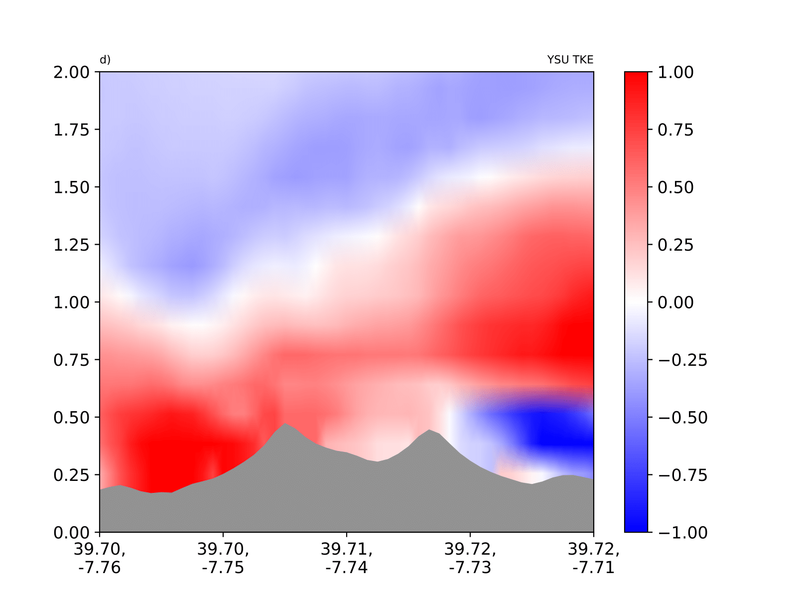
In Figure 5, we looked at the difference from the MYNN TKE scheme for all model results of the daily average wind speed values. Figure 5a shows the result of the MYNN TKE model simulation of the transects of average wind speed for the northeastern flow. In the first column we show the differential results of the TKE parameter, in the second column the areal differentials of the SMAG parameter and in the third column of the NBA model.
The first line shows PBL schemes of MYNN parameter, the second line shows the YSU parameter, and the third line shows the area differences of the SH parameter from the MYNN TKE parameter. When the transect differences for different PBL schemes of the TKE model from the LES parameters are examined, Figure 5d the YSU and SH parameters on the windward side showed higher wind speed values, as shown in the graph, whereas the MYNN parameter in the valley and on the leeward side had higher wind speed values. The YSU parameter results showed more changes in the positive and negative side of the field.
When the transect results of the MYNN parameterization for different LES parameters Figure 5b and 5c are examined, they showed higher wind speed values at windward side and in the valley compared to the SMAG and NBA parameterizations. The MYNN TKE parameterization on the leeward side of the second hill showed higher wind speed values. The MYNN TKE parameterization indicates higher wind speed at both peaks in the northeastern flow, but lower wind speed values inside the valley. The MYNN parameterization has contributed more to the flow on the leeward side in different SGS models. In the northeastern flow, the change in wind speed at the second hill is stronger than at the first hill.
For YSU parameterization are examined, a strong flow on the windward side is observed in all SGS models. In the YSU SMAG parameterization, the value of wind speed at the windward side is stronger than the other two SGS models. When examining the results of SH parameterization (Figure 5g-i) MYNN generally showed results more like the PBL parameter than the YSU parameter. The change in wind speed in the SMAG parameterization is stronger, while the change in the NBA model is more limited. The microscale model successfully reproduced several key characteristics of the flow dynamics at the study site, including wave-like patterns associated with nocturnal low-level jets (LLJ), such as the standing wave observed on the lee side of the ridge during specific wind conditions. The LLJ’s fine details were not fully captured, probably due to the mesoscale tendencies’ resolution ability.
The most important difference is seen in the valley. The NBA model, the change in wind speed showed higher wind speed values, while in the SMAG model, it showed lower wind speed values than in the TKE model. When we examined the flow at the second peak, the SMAG model showed the lowest change in wind speed. In general, the contribution of both of PBL schemes and LES parameterization to the change is identical when we examine the results. A strong descending flow is generated on the second hill and leeward side by the MYNN TKE parameterization.
Wind speed is also compared with met tower measurements in Figure 6. The modelled wind speed typically follows the observations at 100 m but there is a larger range of variation in the valley than on top of the two ridges.
Figure 7 displays errors quantified in terms of bias. Wind speed errors at 100 m and along the two ridges are changing between -1.5m/s and 3.5 m/s. While the bias errors show negative values at lower part of boundary at both of hill, all models show overprediction on the top of measurement. Within the valley, wind speed errors are on the order of 4 m/s and 1.2 m/s, respectively. While the errors have overprediction at 10 m, error rate decreases as you start to move away from the surface. The model captures the wind speed fluctuations more effectively in the valley than in the ridges, considering the wind speeds present on the second hill. The presence of this contradiction indicates that Mast 25 is located below the mountain wave and in a region of more well-mixed and coherent turbulence.
3.3. Southwestern Flow
WRF runs are used to test the ability of the model to reproduce the flow situation over complex terrain. Three different PBL schemes can be compared with 100m wind speed using the Taylor diagrams in Figure 8. It can be observed that the normalised standardized deviation and correlation coefficient have more error and low correlation for both of hills with decreasing average wind speeds. The correlation of all the PBL schemes at the second hill (Mast 29) is higher than at Mast 20. The MYNN scheme models wind speeds at both of measurement locations better than the other two PBL schemes as seen in northeastern flow pattern results.
Figure 9 show averaged flows of cross-valley wind speed simulations of domain D3. All models accurately replicate the flow pattern approaching the double ridge from the southwest. The simulated and observed single point findings show a high level of agreement. The configuration of the airflow, particularly the atmospheric layers near the surface, exhibit notable disparities when comparing simulations employing distinct parameterization techniques. The flow fails to adequately detach from the surface, resulting in weak or non-existent recirculation zones. The inconsistencies can be partially attributed to incorrect and diminished surface friction.
Figure 9 shows average wind speed values and average vertical wind component values at 10 m and 100 m. The average speed of the southwest wind flow is lower than that of the northeast wind, and the average wind speed of 100 m is less pronounced in all models. Topographic effects have less effect, especially in the entire flow area at 100 m. For the northeast flow, the wind speed on the hill behind the flow has spread to a wider area. The results at 10 m show a strong wind field on the windward side of the Mast 20 measurement point in both the SMAG and the NBA models. This strong wind field creates a limited flow area due to the inadequate resolution of the model topography. There is no such flow area in the 100 m altitude results.
We looked at the difference Figure 10. from the MYNN TKE parameterization for all model results of the average wind speed values. Figure 8a shows the result of the MYNN TKE model simulation of the transects of average wind speed for the southwestern flow. When examining the field difference results for different PBL schemes of the TKE model from the LES parameters, (Figure 10d) the change in the YSU and SH parameterization varies area-by-area, as shown in the graph. In the YSU parameterization, YSU showed higher wind speed in the valley and on the leeward side, while in the SH parameterisation, higher valley wind speed values are observed. When the areal results of the MYNN parameter for different LES parameters Figure 10b and 10c are examined, they showed lower wind speed values over windward, leeward and in the valley compared to the SMAG and NBA parameterization, while MYNN TKE parameterization on both hills showed higher wind speed values. In the southwestern flow, the change in wind speed at the second hill is more severe than at the first hill.
When the results for YSU parameterization are examined, strong flow on the windward are observed in TKE and SMAG models, while lower wind speed values are observed on the SMAG model. In the YSU and SMAG parameterization, the change in wind speed in the wind ward and in the valley is stronger in YSU parameterisation.
The results of SH parameterization are examined, (Figure 10g, 10h and 10i) generally showed more similar results to the YSU parameter. The change over the wind showed lower wind speed values in TKE and SMAG parameters compared to the MYNN TKE model, while the change in wind speed in the NBA model showed higher wind speed values. When we looked at the flow on both hills, it showed the lowest change in wind speed in all SGS models. When, we look at the results in general, the contribution of both the PBL parameters and the LES parameters to the change is similar.
Wind speed is also compared with met tower measurements in Figure 11. The modelled wind speed generally follows the observations at 100 m, with greater variability and fluctuations in the valley and on top of the two ridges. All the models capture the general flow pattern all day, expect the midday all models fluctuate much more. Figure 12 displays errors quantified in terms of bias for the southeastern flow. At 100 m and along the two ridges, wind speed errors are changing between -0.75m/s and 1 m/s. Wind speed errors in the valley are around 3 m/s and 1.5 m/s. While the model overpredicts at 10 m, error rate decreases as you start to move away from the surface. Only second hill has negative errors at lower part of boundary layer, it shows overprediction at the upper part of boundary layer.
We looked at the 100 m boxplot results of 9 different simulations at 3 different observation stations in Figure 13. In this boxplot study, we tried to see the differences in more detail by dividing the one-day simulation into diurnal cycle. At daily cycle in the southwestern flow, all model simulations yield closer results, while in the northeast flow, the contradiction is greater at the measurement station in the southeast hill. Again, the station in the valley exhibits significantly more inconsistencies compared to the observations.
Based on the resolution of both the terrain and land-use data, as well as the capability to resolve turbulent flow structures, nested WRF–LES simulations produce progressively more comprehensive flow predictions. The power spectral density of the 100 m wind speed signals in Figure 12 can be used to detect higher-frequency turbulence as grid resolution increases throught analysis. The spectra of d03 exhibit an inertial subrange and possess energy content congruent with the data.
The wind speed spectra in d02 exhibit a drop-off, which is characteristic of models that use finite difference discretization method. Table 4 shows the error metrics at Mast 20 and Mast 25. The consistency of the bias and RMSE values between the two domains suggests that there is no substantial decrease in errors at the Mast 20 position when nesting to a higher grid resolution. The inaccuracies mostly arise from the steady background flow, which remains rather constant across the domains. Although the recirculation zone is clearly defined on d03, the less steep resolved slopes d02 do not cause recirculation in same areas. Enhanced grid resolution and terrain resolution have a direct impact on d03, resulting in a more precise depiction of the observed flow characteristics at Mast 25 position.
In general, LES results show better outcomes in unstable conditions, while in stable conditions, it has not demonstrated a very good approach in solving turbulent flow.
4. Conclusions
This study used a comprehensive WRF-LES model to replicate a 36-h real weather scenario in the Perdigão region at 19-20 May 2017 and 13-14 June 2017. The averaged meteorological aspects and statistical properties of the flow are strongly correlated during IOP verifications.
Creating a high-performance microscale atmospheric simulation requires the use of high-quality topography data. The efficiency of high-resolution modelling is increased by using high-resolution topographic data. The WRF-LES model exhibits the capability to accurately depict the diverse surface fluxes and small-scale circulations within the relevant ares, such as the mountanious Perdigão region.
The present work also aims to examine the uncertainty of various planetary boundary layer (PBL) treatments at the gray zone scales. To do this, sensitivity tests using Large Eddy Simulation (LES), Mellor-Yamada-Nakanishi-Niino (MYNN), Yonsei University (YSU), and Simulated Heating (SH) have been conducted, and the findings are compared. Different PBL schemes offer various advantages under different geographical conditions. The YSU scheme performs better in larger areas with less complex topographical structures, particularly in convective movements. On the other hand, the MYNN scheme demonstrates better performance in more complex topographies (such as mountains areas and valleys) and turbulent flows. Although the SH scheme yields better results in turbulent flows within mountainous and complex terrains, it requires high resolution and high computational capacity to achieve this. When we examine the results of our study, despite showing comparable outcomes, the MYNN scheme achieved higher performance due to insufficient resolution for SH modeling in our simulations. To get more effective results, it is necessary for MYNN to have a greater capacity for both nonlocal and local heat transport.
Three distinct SFS models, including basic to advanced methodologies in complex terrain are employed to analyse the effects of horizontal mesh refinement. The two most basic models are linear, constant coefficient eddy-viscosity models, where the eddy viscosity coefficient is determined either using the strain-rate (SMAG) or a 1.5-order prognostic equation for subgrid-scale (SFS) turbulence kinetic energy [17,18]. The Nonlinear Backscatter and Anisotropy (NBA) model, developed by Kosovic ́ in 1997 and further studied by Kosovic ́ & Curry in 2000, is being investigated [76,80]. This model incorporates a nonlinear constitutive connection.
Generally, Large Eddy Simulation (LES) models are more effective than Planetary Boundary Layer (PBL) parameterization techniques when simulating real flow over complex terrain at the gray zone scale. The difference in day-to-night emissions at the Mast 20 measurement station in the NE flow is greater than in the SW flow. At station Mast 20, in the northeastern flow, the difference between night and day is most noticeable. The results in low wind speeds under southwesterly flow show similarity with observations.
Research on the combined performance of Large Eddy Simulation and Planetary Boundary Layer has significantly increased in recent times. We have observed that similar approaches on this subject have been seen simultaneously presented, Large Eddy Simulations being prefered rather than by Planetary Boundary Layer models for better addressing the gray zone [7,81,82,83,84]. The characteristics of the wind field in the lower atmosphere over complex terrain are highly influenced by the choice of planetary boundary layer treatments.
To assess the level of uncertainty in the SGS stress model at the microscale, we evaluate three regularly employed SGS stress models in the LES: 1.5TKE, SMAG, and NBA. On the gray zone scale, each SGS model has a reduced impact on both the simulated average values and statistical measures. On a smaller scale, the impact becomes more pronounced. The stress models developed by SGS have a greater influence compared to the IBCs built using various PBL treatments in the parent gray zone domain.
Out of these models, the NBA model demonstrates the highest level of performance, which aligns with the simulated results conducted by Kirkil, Mirocha, and Zhou & Chow [24,25,85,86,87].
Recently, there has been tremendous progress in the study of the planetary boundary layer (PBL) through measurement campaigns and modeling efforts. A significant amount of effort has been devoted to improving the parameterizations of the PBL in complex terrain [88,89,90,91]. Nevertheless, the PBL is not yet a reliable method for navigating complex terrain. However, despite the positive findings from idealized studies suggesting that LES is highly effective in simulating boundary layer winds (Kosovic ́ & Curry 2000; Mirocha et al. 2010), it is not a flawless solution for complex terrain [24,80].
Additional research should prioritize enhancing the capabilities of the LES model to accurately represent vertical momentum structures in different atmospheric conditions. This study showcases the capabilities of WRF-LES as a valuable instrument for acquiring fresh knowledge about PBL processes in areas with complex topography. The WRF-LES model has great potential for accurately simulating the flow field in complex terrain. Non-linear models solve the effects in the boundary layer better than linear models.
The results of this study are promising and suggest that it could be useful in complex terrain too. The microscale model records the weater patterns that change slowly, which are fed to it by mesoscale tendencies while also including local orographic and surface effects. Although, mesoscale model appears to provide the correct large-scale force, validating them used for coupling is not an easy task, particularly in complex terrain.
It is important to highlight that the findings of this paper are based on a limited number of individual cases of two different flows. Therefore, it is necessary to assess these results using a wider range of case situations and validate them against further observations. Additional research conducted at the Perdigão site may potentially involve analysing and contrasting observed turbulence measurements. This study specifically examines the impact of large-scale synoptic flow on the topography. Additional improvements in modelling, such as the development of parameterization for the gray zone that considers different scales and the implementation of adaptive subgrid-scale stress (SGS) models at higher resolutions, are anticipated to significantly improve the capabilities of multiscale modelling. The incorporation of turbulence, such as through cell perturbation, together with the utilization of more accurate land-use data sets that include improved roughness and forest maps, as well as enhanced soil moisture data, is expected to improve the simulation of the small-scale valley flows in Perdigão in a more realistic manner.
Author Contributions
Conceptualization, E.Y, S.S.M. and G.K.; methodology, E.Y.; software, E.Y.; writing—original draft preparation, E.Y.; writing—review and editing, S.S.M.; writing—review and editing, G.K.; visualization, E.Y.; All authors have read and agreed to the published version of the manuscript.
Funding
This research has been supported by the ITU Coordination Unit for Scientific Research Projects (ITU-BAP)(grant nos. 1016072023) and part of the special issue “Meso-Micro Model Coupling with WRF-LES and High Resolution Wind Filed Determination” (ITU-BAP).
Data Availability Statement
We encourage all authors of articles published in MDPI journals to share their research data. In this section, please provide details regarding where data supporting reported results can be found, including links to publicly archived datasets analyzed or generated during the study. Where no new data were created, or where data is unavailable due to privacy or ethical restrictions, a statement is still required. Suggested Data Availability Statements are available in section “MDPI Research Data Policies” at https://www.mdpi.com/ethics.
Acknowledgments
The Perdigão field campaign was primarily funded by the US National Science Foundation, European Commission’s ERANET+, Danish Energy Agency, German Federal Ministry of Economy and Energy, Portugal Foundation for Science and Technology, US Army Research Laboratory, and the Israel Binational Science Foundation. This study uses the Advanced Research WRF-ARW model and the WRF Preprocessing System (WPS) version 3.8.1 (Boulder, USA). The WRF-ARW and WPS are publicly available at http: //ww2.mmm.ucar.edu/wrf/users/ (accessed on 1 November 2021). Initial and boundary condition data are provided by the ERA-5 reanalysis dataset with 0.3◦ from https://cds.climate.copernicus.eu/ (accessed on 1 November 2021). Land cover and elevation datasets at 30 s resolutions are used and provided from http://www2.mmm. ucar.edu/wrf/src/wps_files/ (accessed on 1 November 2021). Computing resources used in this work were provided by the National Center for High Performance Computing of Turkey (UHeM) under grant number 1016072023. Acknowledgment is due to Fahri Mert Sayınta for his support throughout this study.
Conflicts of Interest
The authors declare no conflicts of interest.
Abbreviations
The following abbreviations are used in this manuscript:
| a.g.l. | above ground level |
| CFD | Computational fluid dynamics |
| CLC | Corine Land Cover |
| CORINE | Coordination of Information on the Environment |
| ECMWF | European Centre for Medium-range Weather Forecast |
| ERA5 | ECMWF Reanalysis 5th generation data |
| GTOPO30 | Global topography at 30 arcsec |
| IBC | Initial boundary condition |
| IOP | Intensive operational period |
| LESLLJ | Large-eddy SimulationLow-level jet |
| MYNN | Mellor-Yamada-Nakanishi-Niino level 2.5 |
| MWR | Microwave radiometers |
| NBA | Nonlinear Backscatter and Anisotropy Model |
| NCAR | National center for atmospheric Research |
| NE | Northeast |
| NEWA | New European Wind Atlas |
| PBL | Planetary Boundary Layer |
| RASS | Radio acoustic sounding system |
| SFS | Subfilter-scale |
| SGS | Sub-grid Scale |
| SH | Shin-Hong |
| SMAG | Smagorinsky Model |
| SRTM | Shuttle Radar Topography Mission |
| SW | Southwest |
| TKE | 1.5-order turbulence kinetic energy closure Model |
| UCAR | University Corporation for Atmospheric Research |
| USGS | United States Geological Survey |
| YSU | Yonsei University |
| WAsP | Wind Atlas Analysis and Application Program |
| WRF | Weather Research and Forecasting (model) |
| WRF-LES | Weather Research and Forecasting & Large-eddy Simulation |
Appendix A
Appendix A.1
In Table A1, the statistical RMSE values of the results are calculated at 3 measurement stations and at 4 different altitudes; the best result for 100m was 1.37 m/s for the station on the northeast hill number Mast 29 using the MYNN NBA model simulation for Northeastern flow. In the measuring station inside the valley, the best result is calculated at with SH TKE simulation. Simulations on both hills show higher wind speeds than observed wind speed values, while lower values have been observed in the valley. More statistical evaluations of model results are shown in Table A1 which gives the 10-min 10 m, 30 m, 60 m and 100 m wind speed comparison in all simulations.

Table A1.
RMSE results of comparisons of WRF–LES (simulations) and meteorological tower measurements (observed data) for the Northeastern and Southwestern flow case studies for wind speed.
Table A1.
RMSE results of comparisons of WRF–LES (simulations) and meteorological tower measurements (observed data) for the Northeastern and Southwestern flow case studies for wind speed.
| PBL SGS z [m a.g.l.] | Mast 20 | Mast 25 | Mast 29 | |||||
|---|---|---|---|---|---|---|---|---|
| NE | SW | NE | SW | NE | SW | |||
| MYNN | TKE | 100 | 3.69 | 2.01 | 4.42 | 3.14 | 1.51 | 1.86 |
| 60 | 3.45 | 1.95 | 3.78 | 2.87 | 2.56 | 1.85 | ||
| 30 | 3.22 | 1.86 | 2.56 | 2.49 | 3.05 | 1.84 | ||
| 10 | 3.13 | 1.77 | 1.63 | 2.07 | 3.85 | 1.82 | ||
| SMAG | 100 | 3.51 | 2.00 | 4.27 | 3.54 | 1.43 | 2.20 | |
| 60 | 3.35 | 1.89 | 3.08 | 3.25 | 2.07 | 2.17 | ||
| 30 | 3.02 | 1.82 | 2.43 | 2.98 | 2.92 | 2.13 | ||
| 10 | 2.88 | 1.68 | 1.80 | 2.73 | 3.99 | 2.11 | ||
| NBA | 100 | 3.48 | 1.94 | 4.83 | 3.07 | 1.35 | 2.21 | |
| 60 | 3.34 | 1.89 | 3.98 | 2.92 | 1.89 | 2.08 | ||
| 30 | 3.13 | 1.82 | 3.05 | 2.78 | 2.67 | 1.99 | ||
| 10 | 2.97 | 1.70 | 2.03 | 2.63 | 3.79 | 1.90 | ||
| SH | TKE | 100 | 3.61 | 2.07 | 4.36 | 3.54 | 1.79 | 1.96 |
| 60 | 3.35 | 2.06 | 3.69 | 3.17 | 2.16 | 1.90 | ||
| 30 | 3.01 | 2.05 | 2.31 | 2.95 | 2.95 | 1.82 | ||
| 10 | 2.72 | 2.05 | 1.34 | 2.27 | 3.72 | 1.76 | ||
| SMAG | 100 | 3.39 | 1.97 | 3.94 | 3.63 | 1.37 | 2.06 | |
| 60 | 3.04 | 1.89 | 2.73 | 3.30 | 2.01 | 2.03 | ||
| 30 | 2.91 | 1.85 | 2.00 | 3.00 | 3.02 | 2.00 | ||
| 10 | 2.48 | 1.80 | 1.42 | 2.74 | 3.79 | 1.98 | ||
| NBA | 100 | 3.37 | 1.90 | 4.64 | 3.27 | 1.46 | 2.10 | |
| 60 | 3.08 | 1.88 | 3.65 | 3.04 | 1.90 | 2.01 | ||
| 30 | 2.96 | 1.84 | 2.13 | 2.92 | 2.45 | 1.95 | ||
| 10 | 2.58 | 1.82 | 1.71 | 2.72 | 3.66 | 1.84 | ||
| YSU | TKE | 100 | 4.00 | 2.06 | 4.23 | 3.80 | 2.36 | 2.18 |
| 60 | 3.48 | 1.94 | 3.58 | 3.48 | 2.95 | 2.09 | ||
| 30 | 3.01 | 1.82 | 2.82 | 2.97 | 3.27 | 1.99 | ||
| 10 | 2.92 | 1.73 | 1.37 | 2.60 | 3.82 | 1.86 | ||
| SMAG | 100 | 3.96 | 1.96 | 4.14 | 3.78 | 2.27 | 2.06 | |
| 60 | 3.65 | 1.90 | 3.56 | 3.35 | 2.79 | 2.00 | ||
| 30 | 3.19 | 1.82 | 2.35 | 3.06 | 3.06 | 1.95 | ||
| 10 | 2.82 | 1.74 | 1.52 | 2.83 | 3.94 | 1.89 | ||
| NBA | 100 | 3.94 | 1.99 | 4.43 | 3.37 | 2.17 | 2.09 | |
| 60 | 3.33 | 1.88 | 3.45 | 3.02 | 2.86 | 2.01 | ||
| 30 | 3.06 | 1.76 | 2.16 | 2.90 | 3.06 | 1.94 | ||
| 10 | 2.87 | 1.68 | 1.65 | 2.72 | 3.55 | 1.82 | ||
References
- Bauer, H. , Weusthoff, T., Dorninger, M., Wulfmeyer, V., Schwitalla, T., Gorgas, T., Arpagaus, M., & Warrach-Sagi, K. Predictive skill of a subset of models participating in D-PHASE in the COPS region. Quarterly Journal of the Royal Meteorological Society 2011, 137, 287–305. [Google Scholar] [CrossRef]
- Schwitalla, T. , Bauer, H., Wulfmeyer, V., & Aoshima, F. High-resolution simulation over central Europe: assimilation experiments during COPS IOP 9c. Quarterly Journal of the Royal Meteorological Society 2011, 137, 156–175. [Google Scholar] [CrossRef]
- Zittis, G. , Bruggeman, A., Camera, C., Hadjinicolaou, P., & Lelieveld, J. The added value of convection permitting simulations of extreme precipitation events over the eastern Mediterranean. Atmospheric Research 2017, 191, 20–33. [Google Scholar] [CrossRef]
- Feng, Z. , Leung, L. R., Houze, R. A., Hagos, S., Hardin, J., Yang, Q., Han, B., & Fan, J. Structure and Evolution of Mesoscale Convective Systems: Sensitivity to Cloud Microphysics in Convection-Permitting Simulations Over the United States. Journal of Advances in Modeling Earth Systems 2018, 10, 1470–1494. [Google Scholar] [CrossRef]
- Martínez, R. I. , & Chaboureau, J. P. Precipitation and Mesoscale Convective Systems: Explicit versus Parameterized Convection over Northern Africa. Monthly Weather Review 2018, 146, 797–812. [Google Scholar] [CrossRef]
- Woodhams, B.J. , Birch, C. Monthly Weather Review 2018.
- Wagner, J. , Gerz, T., Wildmann, N., & Gramitzky, K. Long-term simulation of the boundary layer flow over the double-ridge site during the Perdigão 2017 field campaign. Atmospheric Chemistry and Physics 2019, 19, 1129–1146. [Google Scholar] [CrossRef]
- Muñoz-Esparza, D. , Lundquist, J. K., Sauer, J. A., Kosović, B., & Linn, R. R. Coupled mesoscale-LES modeling of a diurnal cycle during the CWEX-13 field campaign: From weather to boundary-layer eddies. Journal of Advances in Modeling Earth Systems 2017, 9, 1572–1594. [Google Scholar] [CrossRef]
- Wildmann, N. , Kigle, S., & Gerz, T. Coplanar lidar measurement of a single wind energy converter wake in distinct atmospheric stability regimes at the Perdigão 2017 experiment. Journal of Physics: Conference Series 2018, 1037, 052006. [Google Scholar] [CrossRef]
- Wildmann, N. , Bodini, N., Lundquist, J. K., Bariteau, L., & Wagner, J. Estimation of turbulence dissipation rate from Doppler wind lidars and in situ instrumentation for the Perdigão 2017 campaign. Atmospheric Measurement Techniques 2019, 12, 6401–6423. [Google Scholar] [CrossRef]
- Emeis, S. : Wind Energy Meteorology, vol. [CrossRef]
- Jørgensen, H. , Nielsen, M., Barthelmie, R., and Mortensen, N.: Modelling offshore wind resources and wind conditions, in: Proceedings (CD-ROM) Copenhagen Offshore Wind, 26–28 Oc- tober 2005, https://backend.orbit.dtu.dk/ws/portalfiles/portal/ 107919793/Modelling_offshore_wind_resources_and_wind_ conditions.pdf (last access: ), 2005. 10 January.
- Blocken, B. : 50 years of Computational Wind Engineering: Past, present and future, J. Wind Eng. Ind. Aerod. 2014, 129, 69–102. [Google Scholar] [CrossRef]
- Skamarock, W. C. , Klemp, J. B., Dudhia, J., Gill, D. O., Barker, D. M., Wang, W., and Powers, J. G.: A description of the advanced research WRF version 3, Tech. rep., NCAR, https://opensky.ucar.edu/islandora/object/technotes:500, 2008.
- Nakanishi, M. , & Niino, H. An Improved Mellor–Yamada Level-3 Model: Its Numerical Stability and Application to a Regional Prediction of Advection Fog. Boundary-Layer Meteorology 2006, 119, 397–407. [Google Scholar] [CrossRef]
- Hong, S. Y. , Noh, Y., & Dudhia, J. A New Vertical Diffusion Package with an Explicit Treatment of Entrainment Processes. Monthly Weather Review 2006, 134, 2318–2341. [Google Scholar] [CrossRef]
- Smagorınsky, J. General Cırculatıon Experıments Wıth The Prımıtıve Equatıons. Monthly Weather Review 1963, 91, 99–164. [Google Scholar] [CrossRef]
- Lilly, D. K. On the application of the eddy viscosity concept in the inertial sub-range of turbulence. NCAR Manuscript 1966, 123, 19. [Google Scholar] [CrossRef]
- Lilly, D. K. , 1967: The representation of small-scale turbulence in numerical experiment. Proc. IBM Scientific Computing Symp. on Environmental Sciences, White Plains, NY, IBM, 195–210.
- Pope, S. B. Ten questions concerning the large-eddy simulation of turbulent flows. New Journal of Physics 2004, 6, 35–35. [Google Scholar] [CrossRef]
- Stoll, R. , Gibbs, J. A., Salesky, S. T., Anderson, W., & Calaf, M. Large-Eddy Simulation of the Atmospheric Boundary Layer. Boundary-Layer Meteorology 2020, 177, 541–581. [Google Scholar] [CrossRef]
- Shaw, R. H. , & Schumann, U. Large-eddy simulation of turbulent flow above and within a forest. Boundary-Layer Meteorology 1992, 61, 47–64. [Google Scholar] [CrossRef]
- Quimbayo-Duarte, J. , Wagner, J., Wildmann, N., Gerz, T., & Schmidli, J. Evaluation of a forest parameterization to improve boundary layer flow simulations over complex terrain. A case study using WRF-LES V4.0.1. Geoscientific Model Development 2022, 15, 5195–5209. [Google Scholar] [CrossRef]
- Mirocha, J. D. , Lundquist, J. K., & Kosović, B. Implementation of a Nonlinear Subfilter Turbulence Stress Model for Large-Eddy Simulation in the Advanced Research WRF Model. Monthly Weather Review 2010, 138, 4212–4228. [Google Scholar]
- Kirkil, G. , Mirocha, J., Bou-Zeid, E., Chow, F. K., & Kosović, B. Implementation and Evaluation of Dynamic Subfilter-Scale Stress Models for Large-Eddy Simulation Using WRF*. Monthly Weather Review 2012, 140, 266–284. [Google Scholar] [CrossRef]
- Deardorff, J. W. A numerical study of three-dimensional turbulent channel flow at large Reynolds numbers. Journal of Fluid Mechanics 1970, 41, 453–480. [Google Scholar] [CrossRef]
- Deardorff, J. W. Numerical Investigation of Neutral and Unstable Planetary Boundary Layers. Journal of the Atmospheric Sciences 1972, 29, 91–115. [Google Scholar] [CrossRef]
- Deardorff, J. W. Stratocumulus-capped mixed layers derived from a three-dimensional model. Boundary-Layer Meteorology 1980, 18, 495–527. [Google Scholar] [CrossRef]
- Moeng, C. H. A Large-Eddy-Simulation Model for the Study of Planetary Boundary-Layer Turbulence. Journal of the Atmospheric Sciences 1984, 41, 2052–2062. [Google Scholar] [CrossRef]
- Chlond, A. , & Wolkau, A. Large-Eddy Simulation Of A Nocturnal Stratocumulus-Topped Marine Atmospheric Boundary Layer: An Uncertainty Analysis. Boundary-Layer Meteorology 2000, 95, 31–55. [Google Scholar] [CrossRef]
- Raasch, S. , & Schröter, M. PALM - A large-eddy simulation model performing on massively parallel computers. Meteorologische Zeitschrift 2001, 10, 363–372. [Google Scholar] [CrossRef]
- Heinze, R. , Dipankar, A., Henken, C. C., Moseley, C., Sourdeval, O., Trömel, S., Xie, X., Adamidis, P., Ament, F., Baars, H., Barthlott, C., Behrendt, A., Blahak, U., Bley, S., Brdar, S., Brueck, M., Crewell, S., Deneke, H., Di Girolamo, P.,... Quaas, J. Large-eddy simulations over Germany using ICON: a comprehensive evaluation. Quarterly Journal of the Royal Meteorological Society 2017, 143, 69–100. [Google Scholar] [CrossRef]
- Talbot, C. , Bou-Zeid, E., & Smith, J. Nested Mesoscale Large-Eddy Simulations with WRF: Performance in Real Test Cases. Journal of Hydrometeorology 2012, 13, 1421–1441. [Google Scholar] [CrossRef]
- Powers, J. G. , and Coauthors, : The Weather Research and Forecasting Model: Overview, system efforts, and future directions. Bull. Amer. Meteor. Soc. 2017, 98, 1717–1737. [Google Scholar] [CrossRef]
- Catalano, F. , & Moeng, C. H. Large-Eddy Simulation of the Daytime Boundary Layer in an Idealized Valley Using the Weather Research and Forecasting Numerical Model. Boundary-Layer Meteorology 2010, 137, 49–75. [Google Scholar] [CrossRef]
- Taylor, D. M. , Chow, F. K., Delkash, M., & Imhoff, P. T. Numerical simulations to assess the tracer dilution method for measurement of landfill methane emissions. Waste Management 2016, 56, 298–309. [Google Scholar] [CrossRef] [PubMed]
- Klemp, J. B. , Skamarock, W. C., & Fuhrer, O. Numerical Consistency of Metric Terms in Terrain-Following Coordinates. Monthly Weather Review 2003, 131, 1229–1239. [Google Scholar] [CrossRef]
- Mahrer, Y. An Improved Numerical Approximation of the Horizontal Gradients in a Terrain-Following Coordinate System. Monthly Weather Review 1984, 112, 918–922. [Google Scholar] [CrossRef]
- Schär, C. , Leuenberger, D., Fuhrer, O., Lüthi, D., & Girard, C. A New Terrain-Following Vertical Coordinate Formulation for Atmospheric Prediction Models. Monthly Weather Review 2002, 130, 2459–2480. [Google Scholar] [CrossRef]
- Zängl, G. An Improved Method for Computing Horizontal Diffusion in a Sigma-Coordinate Model and Its Application to Simulations over Mountainous Topography. Monthly Weather Review 2002, 130, 1423–1432. [Google Scholar] [CrossRef]
- Zängl, G. , Gantner, L., Hartjenstein, G., & Noppel, H. Numerical errors above steep topography: A model intercomparison. Meteorologische Zeitschrift 2004, 13, 69–76. [Google Scholar] [CrossRef]
- Salmon, J. , Bowen, A., Hoff, A., Johnson, R., Mickle, R., Taylor, P., Tetzlaff, G., and Walmsley, J.: The Askervein Hill Project: Mean wind variations at fixed heights above ground. Bound.-Lay. Me- teorol. 1988, 43, 247–271. [Google Scholar] [CrossRef]
- Bechmann, A. , Berg, J., Courtney, M., Jørgensen, H., Mann, J., and Sørensen, N.: The Bolund Experiment: Blind Comparison of Models for Wind in Complex Terrain (Invited), American Geo- physical Union (AGU) Fall Meeting Abstracts, https://ui.adsabs. harvard.edu/abs/2009AGUFM.A33H..08B/abstract (last access: ), 2009. 10 January.
- Rodrigo, J. , Santos, P., Chavez, R., Avila, M., Cavar, D., Lehmkuhl, O., Owen, H., Li, R., and Tromeur, E.: The ALEX17 diurnal cycles in complex terrain benchmark. J. Phys.-Conf. Ser. 2021, 1934, 012002. [Google Scholar] [CrossRef]
- Fernando, H. J. S. , Mann, J., Palma, J. M. L. M., Lundquist, J. K., Barthelmie, R. J., Belo-Pereira, M., Brown, W. O. J., Chow, F. K., Gerz, T., Hocut, C. M., Klein, P. M., Leo, L. S., Matos, J. C., On- cley, S. P., Pryor, S. C., Bariteau, L., Bell, T. M., Bodini, N., Carney, M. B., Courtney, M. S., Creegan, E. D., Dimitrova, R., Gomes, S., Hagen, M., Hyde, J. O., Kigle, S., Krishnamurthy, R., Lopes, J. C., Mazzaro, L., Neher, J. M. T., Menke, R., Mur- phy, P., Oswald, L., Otarola-Bustos, S., Pattantyus, A. K., Ro- drigues, C. V., Schady, A., Sirin, N., Spuler, S., Svensson, E., Tomaszewski, J., Turner, D. D., van Veen, L., Vasiljevic ́, N., Vas- sallo, D., Voss, S., Wildmann, N., and Wang, Y.: The Perdigão: Peering into Microscale Details of Mountain Winds, B. Am. Meteorol. Soc. 2019, 100, 799–819. [Google Scholar] [CrossRef]
- Menke, R. , Vasiljević, N., Hansen, K. S., Hahmann, A. N., & Mann, J. Does the wind turbine wake follow the topography? A multi-lidar study in complex terrain. Wind Energy Science 2018, 3, 681–691. [Google Scholar] [CrossRef]
- Menke, R. , Vasiljević, N., Mann, J., & Lundquist, J. K. Characterization of flow recirculation zones at the Perdigão site using multi-lidar measurements. Atmospheric Chemistry and Physics 2019, 19, 2713–2723. [Google Scholar] [CrossRef]
- Menke, R. , Vasiljević, N., Wagner, J., Oncley, S. P., & Mann, J. Multi-lidar wind resource mapping in complex terrain. Wind Energy Science 2020, 5, 1059–1073. [Google Scholar] [CrossRef]
- Barthelmie, R. J. , & Pryor, S. C. Automated wind turbine wake characterization in complex terrain. Atmospheric Measurement Techniques 2019, 12, 3463–3484. [Google Scholar] [CrossRef]
- Wyngaard, J. C. Toward Numerical Modeling in the “Terra Incognita. ” Journal of the Atmospheric Sciences 2004, 61, 1816–1826. [Google Scholar] [CrossRef]
- Honnert, R. , Masson, V., & Couvreux, F. A Diagnostic for Evaluating the Representation of Turbulence in Atmospheric Models at the Kilometric Scale. Journal of the Atmospheric Sciences 2011, 68, 3112–3131. [Google Scholar] [CrossRef]
- Boutle, I. A. , Eyre, J. E. J., & Lock, A. P. Seamless Stratocumulus Simulation across the Turbulent Gray Zone. Monthly Weather Review 2014, 142, 1655–1668. [Google Scholar] [CrossRef]
- Efstathiou, G. A. , Beare, R. J., Osborne, S., & Lock, A. P. Grey zone simulations of the morning convective boundary layer development. Journal of Geophysical Research: Atmospheres 2016, 121, 4769–4782. [Google Scholar] [CrossRef]
- Honnert, R. Representation of the grey zone of turbulence in the atmospheric boundary layer. Advances in Science and Research 2016, 13, 63–67. [Google Scholar] [CrossRef]
- Chow, F. , Schär, C., Ban, N., Lundquist, K., Schlemmer, L., & Shi, X. Crossing Multiple Gray Zones in the Transition from Mesoscale to Microscale Simulation over Complex Terrain. Atmosphere 2019, 10, 274. [Google Scholar] [CrossRef]
- Zhou, B. , Simon, J. S., & Chow, F. K. The Convective Boundary Layer in the Terra Incognita. Journal of the Atmospheric Sciences 2014, 71, 2545–2563. [Google Scholar] [CrossRef]
- Zhou, B. , Xue, M., & Zhu, K. A Grid-Refinement-Based Approach for Modeling the Convective Boundary Layer in the Gray Zone: A Pilot Study. Journal of the Atmospheric Sciences 2017, 74, 3497–3513. [Google Scholar] [CrossRef]
- UCAR/NCAR – Earth Observing Laboratory: NCAR/EOL Quality Controlled High-rate ISFS surface flux data, geographic coordi- nate, tilt corrected, Version 1. [CrossRef]
- UCAR/NCAR – Earth Observing Laboratory: NCAR/EOL Quality Controlled 5-min ISFS surface flux data, geographic coordi- nate, tilt corrected, Version 1. [CrossRef]
- Haupt, S. E. , Kosovic, B., Shaw, W., Berg, L. K., Churchfield, M., Cline, J., Draxl, C., Ennis, B., Koo, E., Kotamarthi, R., Mazzaro, L., Mirocha, J., Moriarty, P., Muñoz-Esparza, D., Quon, E., Rai, R. K., Robinson, M., & Sever, G. On Bridging A Modeling Scale Gap: Mesoscale to Microscale Coupling for Wind Energy. Bulletin of the American Meteorological Society 2019, 100, 2533–2550. [Google Scholar] [CrossRef]
- Muñoz-Esparza, D. , & Kosović, B. Generation of Inflow Turbulence in Large-Eddy Simulations of Nonneutral Atmospheric Boundary Layers with the Cell Perturbation Method. Monthly Weather Review 2018, 146, 1889–1909. [Google Scholar] [CrossRef]
- Cai, X. , Yang, Z., Xia, Y., Huang, M., Wei, H., Leung, L. R., & Ek, M. B. Assessment of simulated water balance from Noah, Noah-MP, CLM, and VIC over CONUS using the NLDAS test bed. Journal of Geophysical Research: Atmospheres. [CrossRef]
- Chen, F. , & Dudhia, J. Coupling an Advanced Land Surface–Hydrology Model with the Penn State–NCAR MM5 Modeling System. Part I: Model Implementation and Sensitivity. Monthly Weather Review 2001, 129, 569–585. [Google Scholar] [CrossRef]
- Mlawer, E. J. , Taubman, S. J., Brown, P. D., Iacono, M. J., & Clough, S. A. Radiative transfer for inhomogeneous atmospheres: RRTM, a validated correlated-k model for the longwave. Journal of Geophysical Research: Atmospheres 1997, 102, 16663–16682. [Google Scholar] [CrossRef]
- Dudhia, J. Numerical Study of Convection Observed during the Winter Monsoon Experiment Using a Mesoscale Two-Dimensional Model. Journal of the Atmospheric Sciences 1989, 46, 3077–3107. [Google Scholar] [CrossRef]
- Farr, T. G. , Rosen, P. A., Caro, E., Crippen, R., Duren, R., Hensley, S., Kobrick, M., Paller, M., Rodriguez, E., Roth, L., Seal, D., Shaffer, S., Shimada, J., Umland, J., Werner, M., Oskin, M., Burbank, D., and Alsdorf, D.: The shuttle radar topography mission. Rev. Geophys. 2007, 45, RG2004. [Google Scholar] [CrossRef]
- Palma, J. M. L. M. , Silva, C. A. M., Gomes, V. C., Silva Lopes, A., Simões, T., Costa, P., and Batista, V. T. P.: The digital terrain model in the computational modelling of the flow over the Perdigão site: the appropriate grid size. Wind Energ. Sci. 2020, 5, 1469–1485. [Google Scholar] [CrossRef]
- Copernicus Land Monitoring Service: CORINE Land Cover, available at: https://land.copernicus.eu/pan-european/ corine-land-cover, last access:. 15 April.
- Pineda, N. , Jorba, O., Jorge, J., & Baldasano, J. M. Using NOAA AVHRR and SPOT VGT data to estimate surface parameters: application to a mesoscale meteorological model. International Journal of Remote Sensing 2004, 25, 129–143. [Google Scholar] [CrossRef]
- Hahmann, A. N. , Sīle, T., Witha, B., Davis, N. N., Dörenkämper, M., Ezber, Y., García-Bustamante, E., González-Rouco, J. F., Navarro, J., Olsen, B. T., & Söderberg, S. The making of the New European Wind Atlas – Part 1: Model sensitivity. Geoscientific Model Development 2020, 13, 5053–5078. [Google Scholar] [CrossRef]
- Muñoz-Esparza, D. , Kosović, B., García-Sánchez, C., & van Beeck, J. Nesting Turbulence in an Offshore Convective Boundary Layer Using Large-Eddy Simulations. Boundary-Layer Meteorology 2014, 151, 453–478. [Google Scholar] [CrossRef]
- Jiménez, P. A. , & Dudhia, J. Improving the Representation of Resolved and Unresolved Topographic Effects on Surface Wind in the WRF Model. Journal of Applied Meteorology and Climatology 2012, 51, 300–316. [Google Scholar] [CrossRef]
- Liu, Y. , Warner, T., Liu, Y., Vincent, C., Wu, W., Mahoney, B., Swerdlin, S., Parks, K., & Boehnert, J. Simultaneous nested modeling from the synoptic scale to the LES scale for wind energy applications. Journal of Wind Engineering and Industrial Aerodynamics 2011, 99, 308–319. [Google Scholar] [CrossRef]
- Draxl, C. , Worsnop, R. P., Xia, G., Pichugina, Y., Chand, D., Lundquist, J. K., Sharp, J., Wedam, G., Wilczak, J. M., and Berg, L. K.: Mountain waves can impact wind power generation. Wind Energ. Sci. 2021, 6, 45–60. [Google Scholar] [CrossRef]
- Shin, H. H. , & Hong, S. Y. Representation of the Subgrid-Scale Turbulent Transport in Convective Boundary Layers at Gray zone Resolutions. Monthly Weather Review 2015, 143, 250–271. [Google Scholar] [CrossRef]
- Kosovic ́, B. Subgrid-scale modelling for the large-eddy simulation of high-Reynolds-number boundary layers. Journal of Fluid Mechanics 1997, 336, 151–182. [Google Scholar] [CrossRef]
- Cuxart, J. When Can a High-Resolution Simulation Over Complex Terrain be Called LES? Frontiers in Earth Science 2015, 3. [Google Scholar] [CrossRef]
- Xue, L. , Chu, X., Rasmussen, R., Breed, D., & Geerts, B. A Case Study of Radar Observations and WRF LES Simulations of the Impact of Ground-Based Glaciogenic Seeding on Orographic Clouds and Precipitation. Part II: AgI Dispersion and Seeding Signals Simulated by WRF. Journal of Applied Meteorology and Climatology 2016, 55, 445–464. [Google Scholar] [CrossRef]
- Doubrawa, P. , Montornès, A., Barthelmie, R. J., Pryor, S. C., Giroux, G., & Casso, P. Effect of Wind Turbine Wakes on the Performance of a Real Case WRF-LES Simulation. Journal of Physics: Conference Series 2017, 854, 012010. [Google Scholar] [CrossRef]
- Kosović, B. , & Curry, J. A. A Large Eddy Simulation Study of a Quasi-Steady, Stably Stratified Atmospheric Boundary Layer. Journal of the Atmospheric Sciences 2000, 57, 1052–1068. [Google Scholar] [CrossRef]
- Ching, J. , Rotunno, R., LeMone, M., Martilli, A., Kosovic, B., Jimenez, P. A., & Dudhia, J. Convectively Induced Secondary Circulations in Fine-Grid Mesoscale Numerical Weather Prediction Models. Monthly Weather Review 2014, 142, 3284–3302. [Google Scholar] [CrossRef]
- Rai, R. K. , Berg, L. K., Kosović, B., Haupt, S. E., Mirocha, J. D., Ennis, B. L., & Draxl, C. Evaluation of the Impact of Horizontal Grid Spacing in Terra Incognita on Coupled Mesoscale–Microscale Simulations Using the WRF Framework. Monthly Weather Review 2019, 147, 1007–1027. [Google Scholar] [CrossRef]
- Johnson, A. , & Wang, X. Multicase Assessment of the Impacts of Horizontal and Vertical Grid Spacing, and Turbulence Closure Model, on Subkilometer-Scale Simulations of Atmospheric Bores during PECAN. Monthly Weather Review 2019, 147, 1533–1555. [Google Scholar] [CrossRef]
- Wise, A. S. , Neher, J. M. T., Arthur, R. S., Mirocha, J. D., Lundquist, J. K., & Chow, F. K. Meso- to microscale modeling of atmospheric stability effects on wind turbine wake behavior in complex terrain. Wind Energy Science 2022, 7, 367–386. [Google Scholar] [CrossRef]
- Zhou, B. , & Chow, F. K. Turbulence Modeling for the Stable Atmospheric Boundary Layer and Implications for Wind Energy. Flow, Turbulence and Combustion 2011, 88, 255–277. [Google Scholar] [CrossRef]
- Mirocha, J. , Kosović, B., & Kirkil, G. Resolved Turbulence Characteristics in Large-Eddy Simulations Nested within Mesoscale Simulations Using the Weather Research and Forecasting Model. Monthly Weather Review 2014, 142, 806–831. [Google Scholar] [CrossRef]
- Mirocha, J. D. , Kosovic, B., Aitken, M. L., & Lundquist, J. K. Implementation of a generalized actuator disk wind turbine model into the weather research and forecasting model for large-eddy simulation applications. Journal of Renewable and Sustainable Energy. [CrossRef]
- De Wekker, S. F. J. , & Kossmann, M. Convective Boundary Layer Heights Over Mountainous Terrain—A Review of Concepts. Frontiers in Earth Science. [CrossRef]
- Lehner, M. , & Rotach, M. Current Challenges in Understanding and Predicting Transport and Exchange in the Atmosphere over Mountainous Terrain. Atmosphere 2018, 9, 276. [Google Scholar] [CrossRef]
- Goger, B. , Rotach, M. W., Gohm, A., Fuhrer, O., Stiperski, I., & Holtslag, A. A. M. The Impact of Three-Dimensional Effects on the Simulation of Turbulence Kinetic Energy in a Major Alpine Valley. Boundary-Layer Meteorology 2018, 168, 1–27. [Google Scholar] [CrossRef]
- Liu, Y. , Liu, Y., Muñoz-Esparza, D., Hu, F., Yan, C., & Miao, S. Simulation of Flow Fields in Complex Terrain with WRF-LES: Sensitivity Assessment of Different PBL Treatments. Journal of Applied Meteorology and Climatology 2020, 59, 1481–1501. [Google Scholar] [CrossRef]
Figure 1.
Perdigão Terrain.
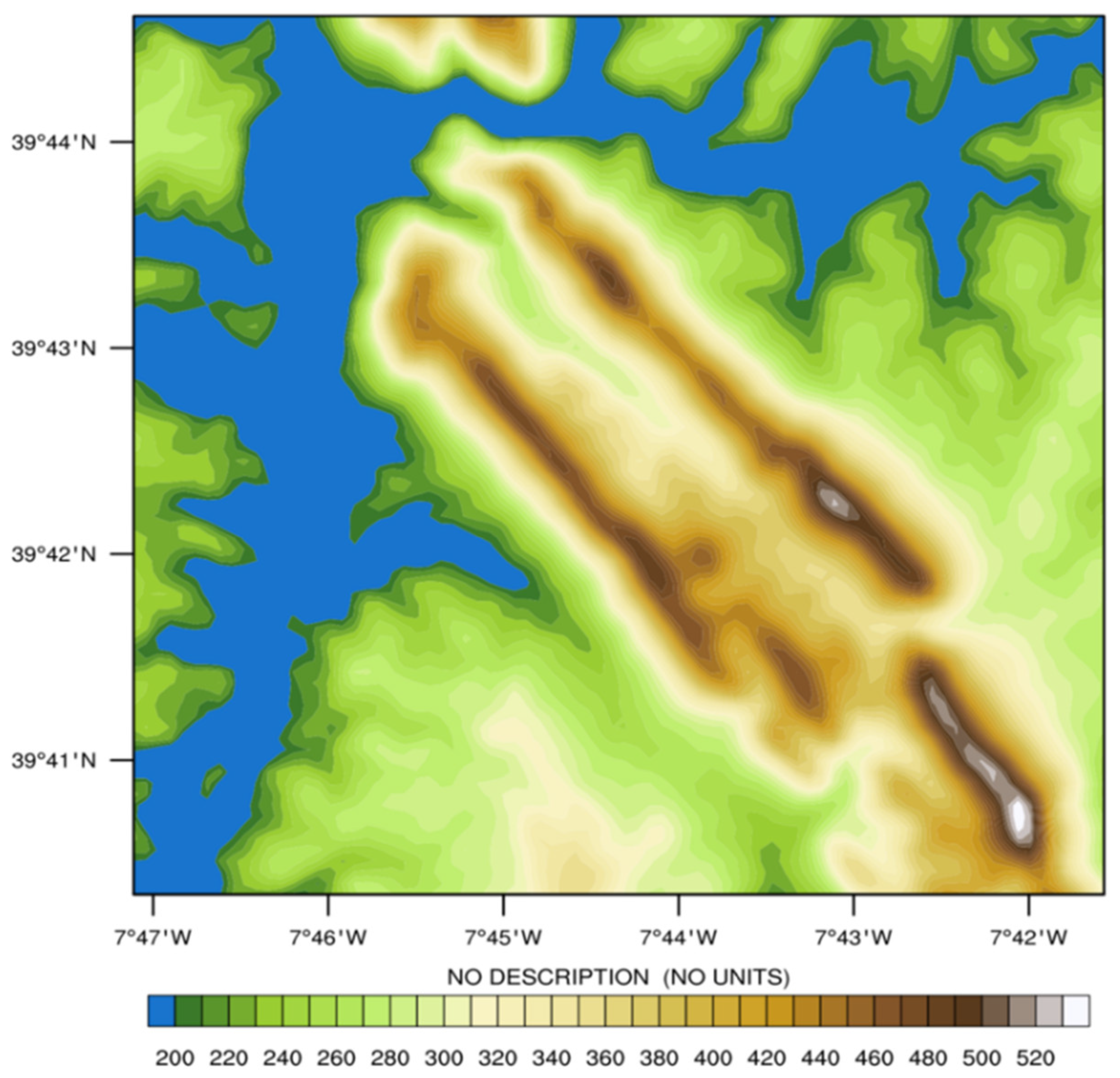
Figure 2.
Topography of domains used in the multi-scale simulation. The three domains have resolutions of 5000 m, 1000 m and 100 m.
Figure 2.
Topography of domains used in the multi-scale simulation. The three domains have resolutions of 5000 m, 1000 m and 100 m.
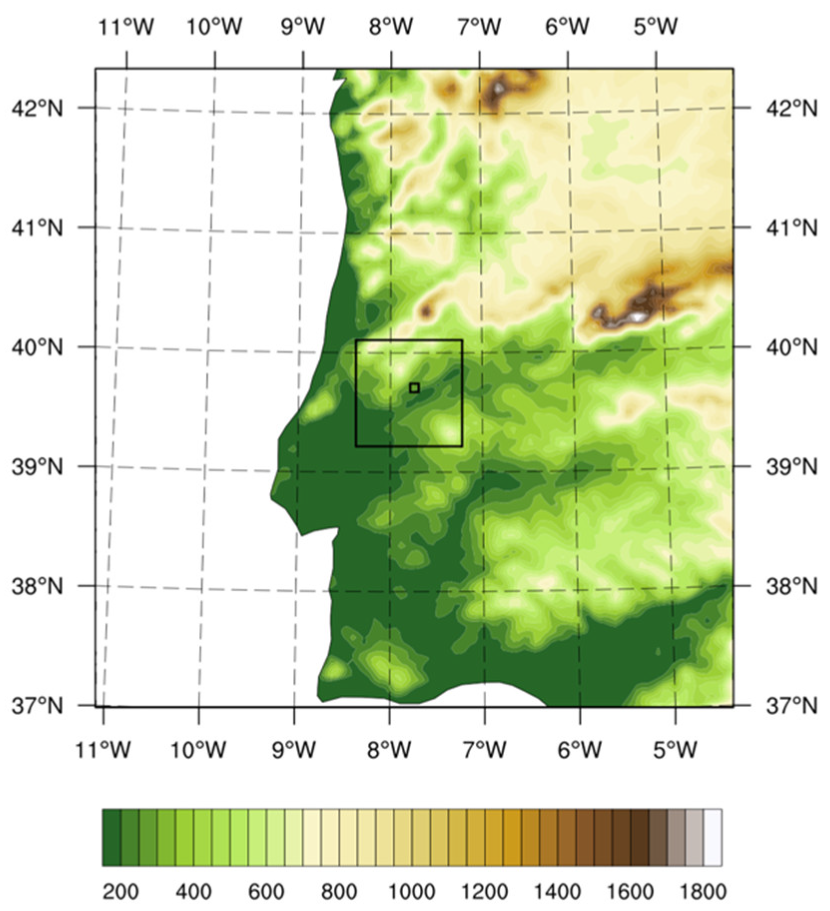
Figure 3.
Taylor diagrams of 100 m northeastern flow wind speeds at Mast 20 (blue dot) and Mast 29 (red dot), comparing observations with simulation results for 3 different PBL parameters in I) MYNN PBL Scheme II) SH PBL Scheme III) YSU PBL Scheme for D02 domain.
Figure 3.
Taylor diagrams of 100 m northeastern flow wind speeds at Mast 20 (blue dot) and Mast 29 (red dot), comparing observations with simulation results for 3 different PBL parameters in I) MYNN PBL Scheme II) SH PBL Scheme III) YSU PBL Scheme for D02 domain.
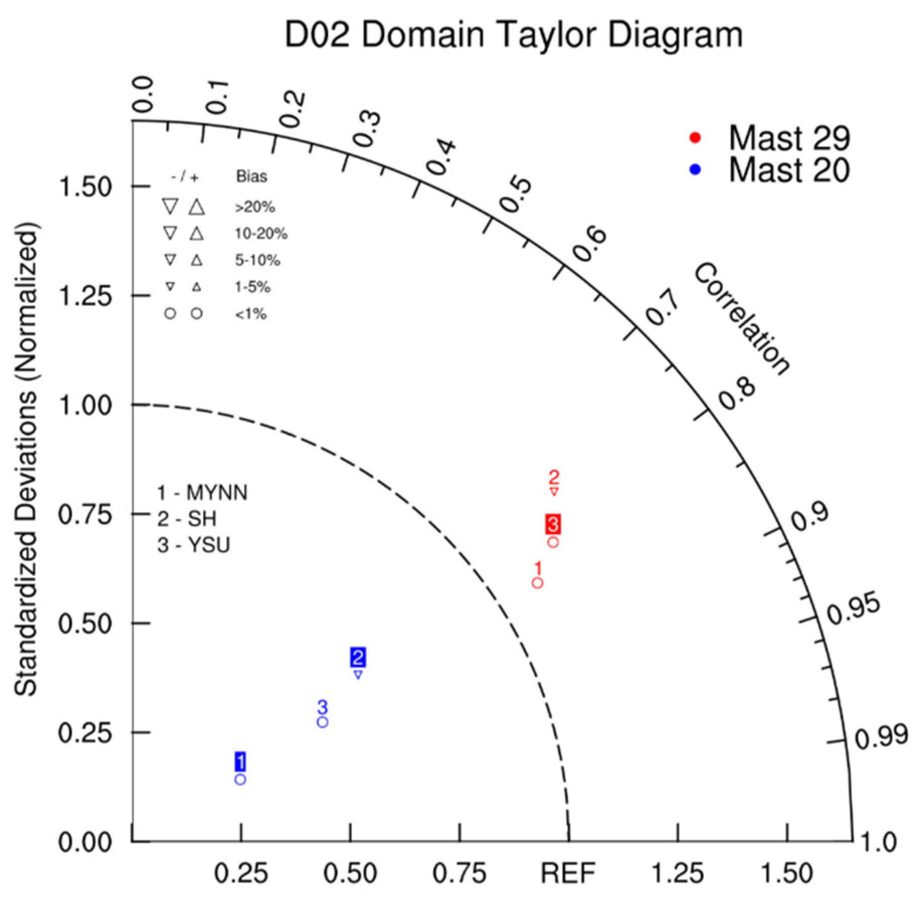
Figure 4.
Average horizontal wind velocity and vertical wind component for 3 different PBL parameters and 3 different LES schemes of the northeast flow I) MYNN PBL Scheme II) YSU PBL Scheme III) SH PBL Scheme for D03 domain. First column is horizontal wind velocity at 10 m, the second column is the vertical wind component at 10 m, the third column is horizontal wind velocity at 100 m and the fourth column is the vertical wind component at 100 m for d03 domain area. The first lines of each PBL parameterizations are TKE model results, the second lines are SMAG model results, and the third lines are NBA model results.
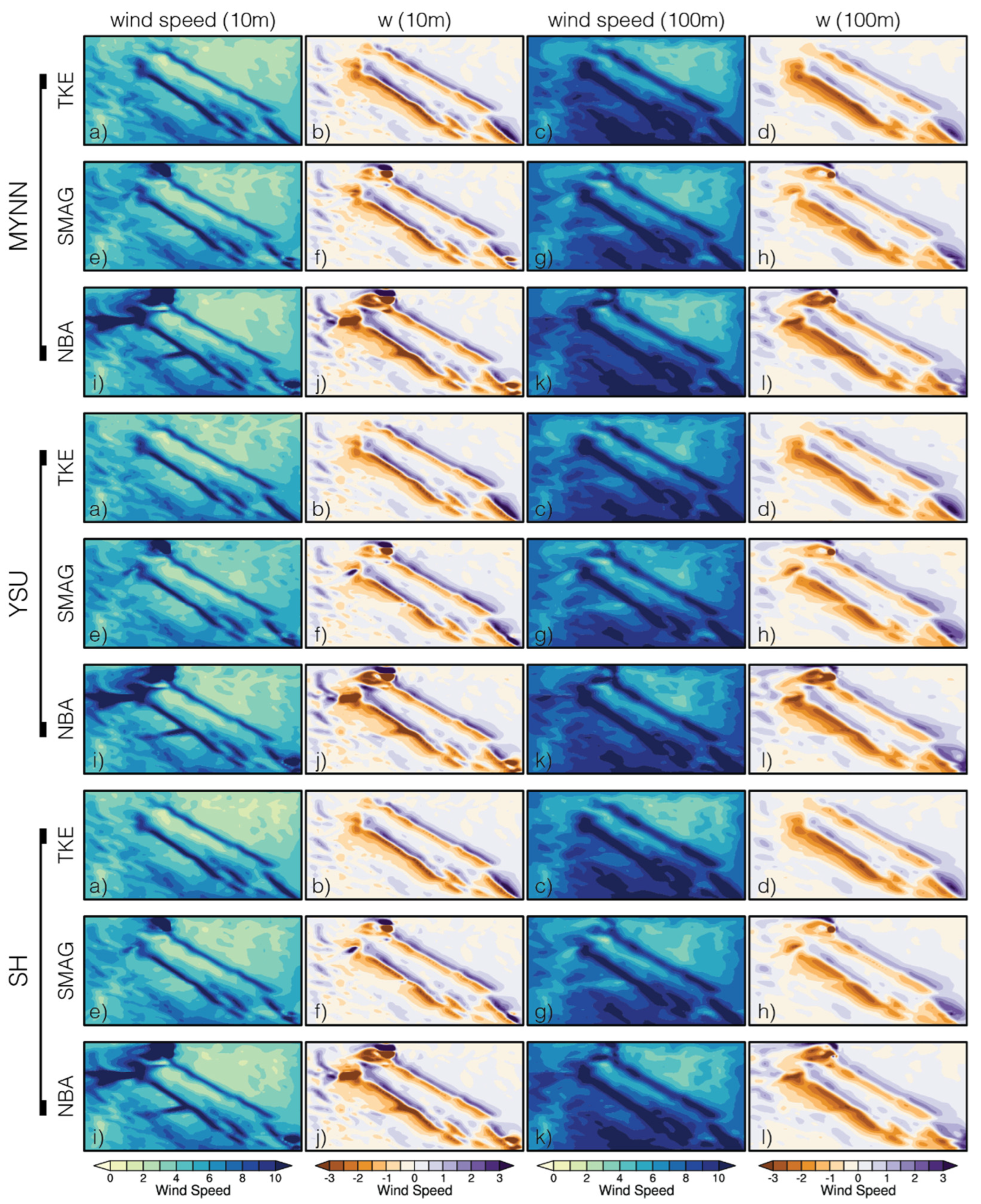
Figure 5.
Transect of one day time-averaged along-transect velocity difference from MYNN TKE model results for b) MYNN SMAG model c) MYNN NBA model d) SH TKE model e) SH SMAG model f) SH NBA modeel e) YSU TKE model f) YSU SMAG model for northeastern flow.
Figure 5.
Transect of one day time-averaged along-transect velocity difference from MYNN TKE model results for b) MYNN SMAG model c) MYNN NBA model d) SH TKE model e) SH SMAG model f) SH NBA modeel e) YSU TKE model f) YSU SMAG model for northeastern flow.
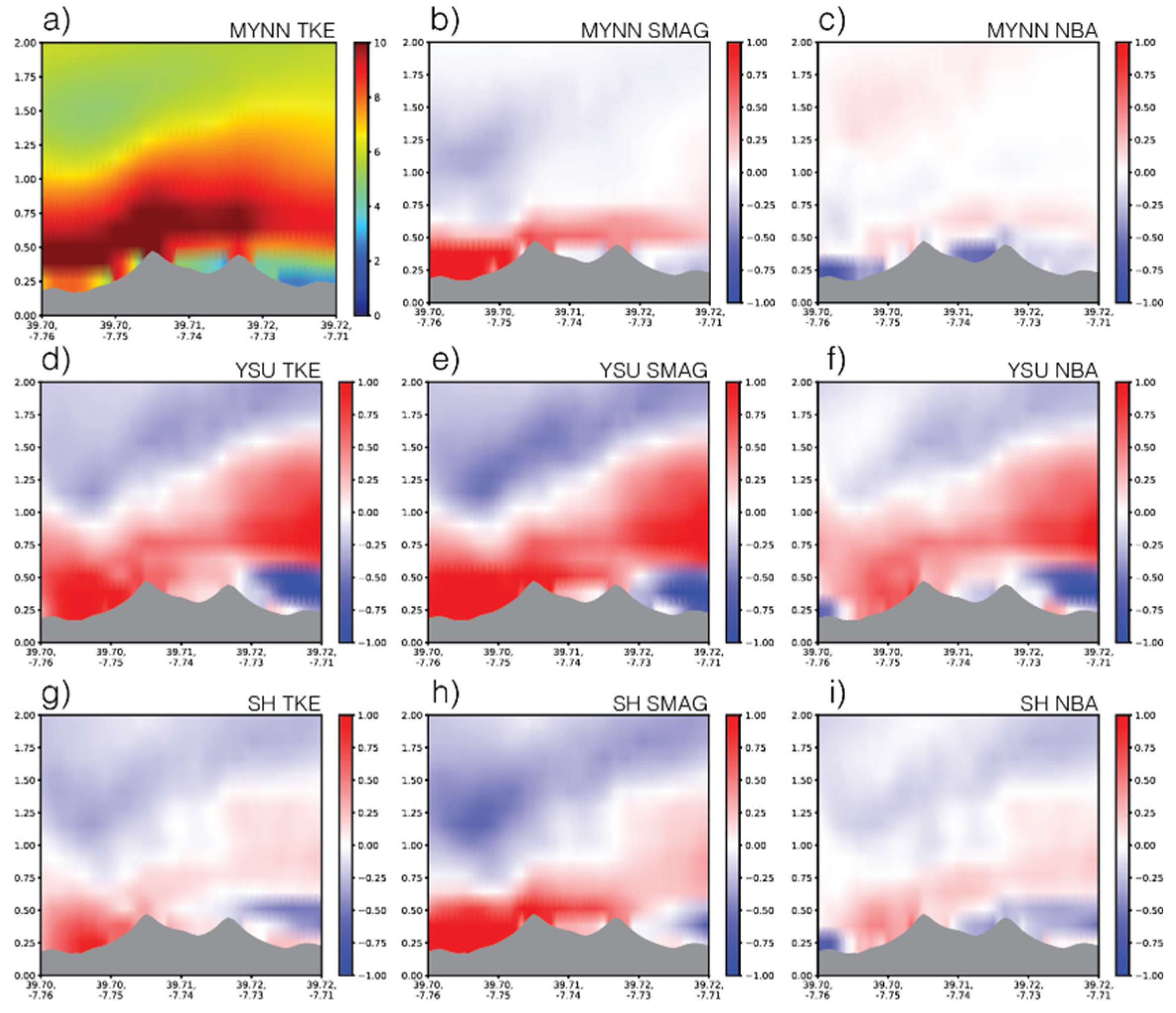
Figure 6.
Time series graphs and comparisons of simulated and observed wind speed at 100m for northeastern flow. First column shows MYNN results, second column show YSU results, and third column show SH results. First row is Mast 20, second row is Mast 25, and third row is Mast 29 results. The black line represents measurement, green line TKE simulation, blue line SMAG simulation and red line NBA simulation.
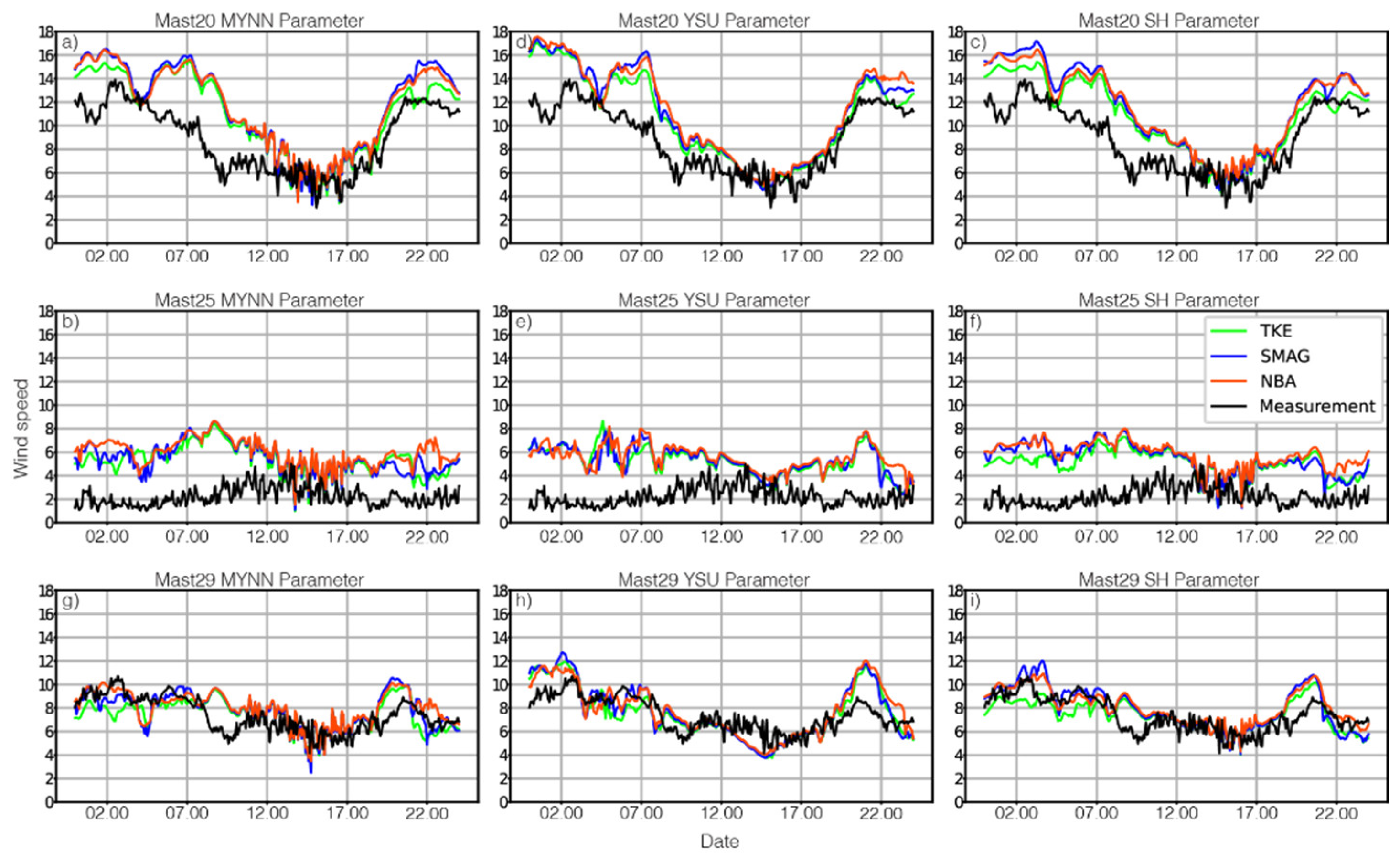
Figure 7.
Wind Speed Bias Results of comparisons of simulated and observed data vertical profile of wind speed a) Mast 20 b) Mast 25 c) Mast 29.
Figure 7.
Wind Speed Bias Results of comparisons of simulated and observed data vertical profile of wind speed a) Mast 20 b) Mast 25 c) Mast 29.
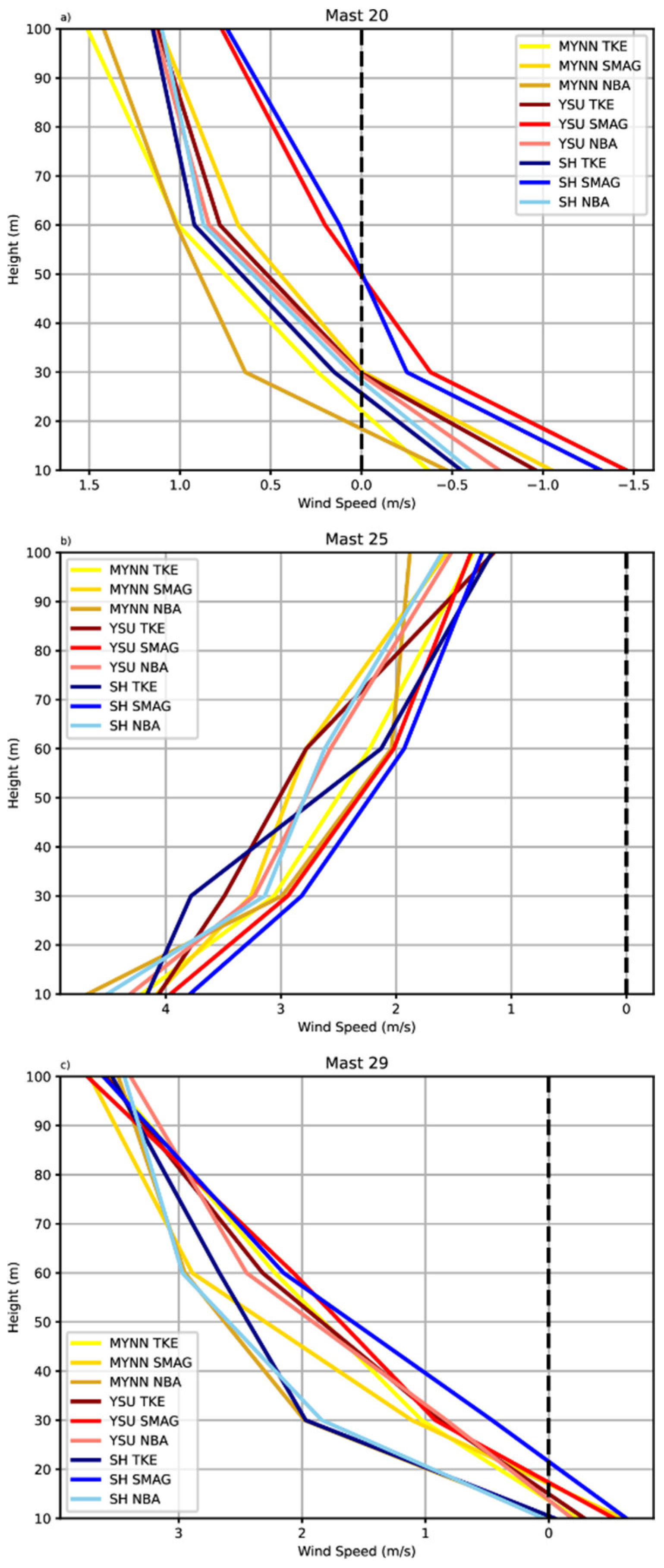
Figure 8.
Taylor diagrams of 100 m southwestern flow wind speeds at Mast 20 (blue dot) and Mast 29 (red dot), comparing observations with simulation results for 3 different PBL parameters in I) MYNN PBL Scheme II) SH PBL Scheme III) YSU PBL Scheme for D02 domain.
Figure 8.
Taylor diagrams of 100 m southwestern flow wind speeds at Mast 20 (blue dot) and Mast 29 (red dot), comparing observations with simulation results for 3 different PBL parameters in I) MYNN PBL Scheme II) SH PBL Scheme III) YSU PBL Scheme for D02 domain.
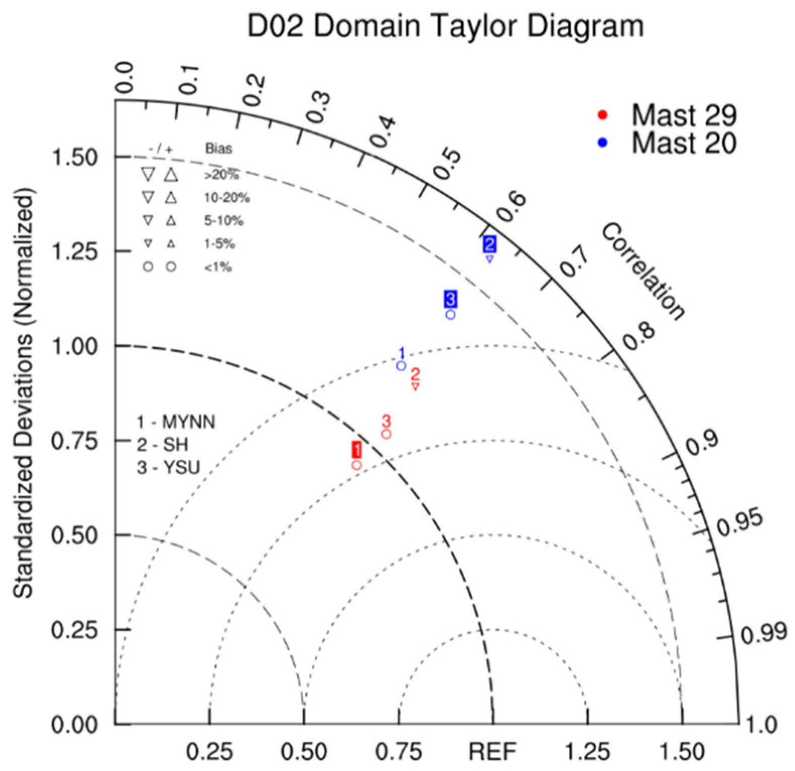
Figure 9.
Average horizontal wind velocity and vertical wind component for 3 different PBL parameters and 3 different LES schemes of the southwestern flow I) MYNN PBL Scheme II) YSU PBL Scheme III) SH PBL Scheme. First columns are horizontal wind velocity at 10 m, the second columns are the vertical wind component at 10 m, the third columns are horizontal wind velocity at 100 m and the fourth columns is the vertical wind component at 100 m for d03 domain area. The first line is TKE model results, the second line is SMAG model results, and the third line is NBA model results.
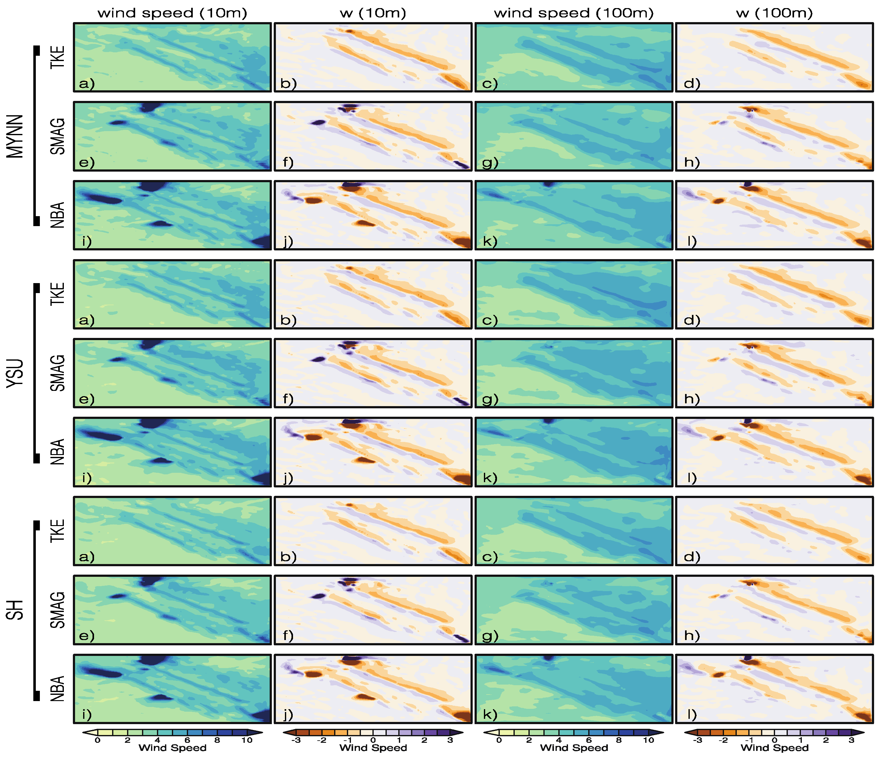
Figure 10.
Transect of one day time-averaged along-transect velocity difference from MYNN TKE model results for b) MYNN SMAG model c) MYNN NBA model d) SH TKE model e) SH SMAG model f) SH NBA modeel e) YSU TKE model f) YSU SMAG model for southwestern flow.
Figure 10.
Transect of one day time-averaged along-transect velocity difference from MYNN TKE model results for b) MYNN SMAG model c) MYNN NBA model d) SH TKE model e) SH SMAG model f) SH NBA modeel e) YSU TKE model f) YSU SMAG model for southwestern flow.
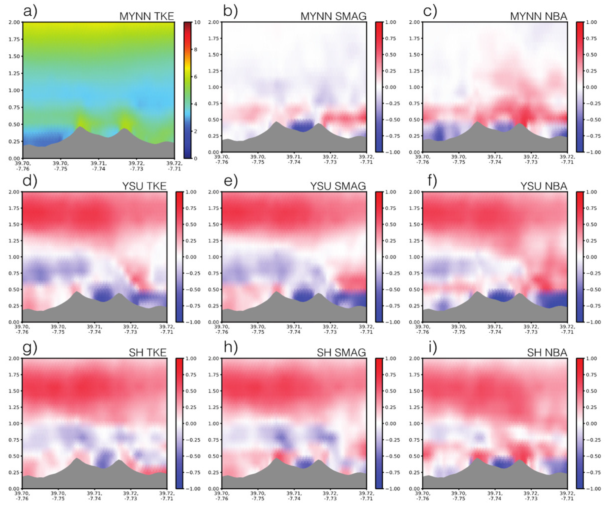
Figure 11.
Time series graphs and comparisons of simulated and observed wind speed at 100m for southwestern flow. First column shows MYNN results, second column show YSU results, and third column show SH results. First row is Mast 20, second row are Mast 25, and third row are Mast 29 results. The black line represents measurement, green line TKE simulation, blue line SMAG simulation and red line NBA simulation.
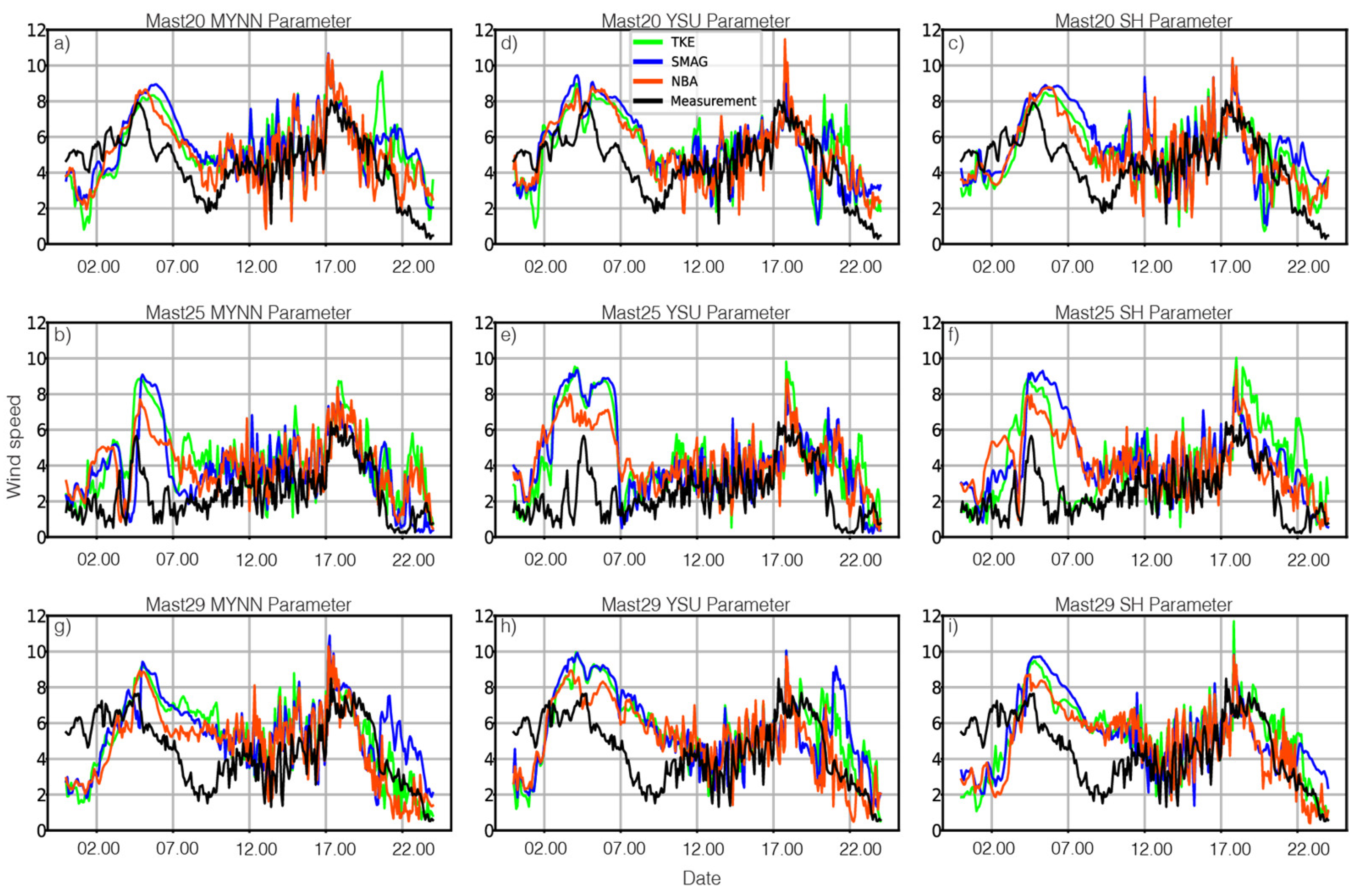
Figure 12.
Wind Speed Bias Results of comparisons of simulated and observed data vertical profile of wind speed a) Mast 20 b) Mast25 c) Mast29.
Figure 12.
Wind Speed Bias Results of comparisons of simulated and observed data vertical profile of wind speed a) Mast 20 b) Mast25 c) Mast29.
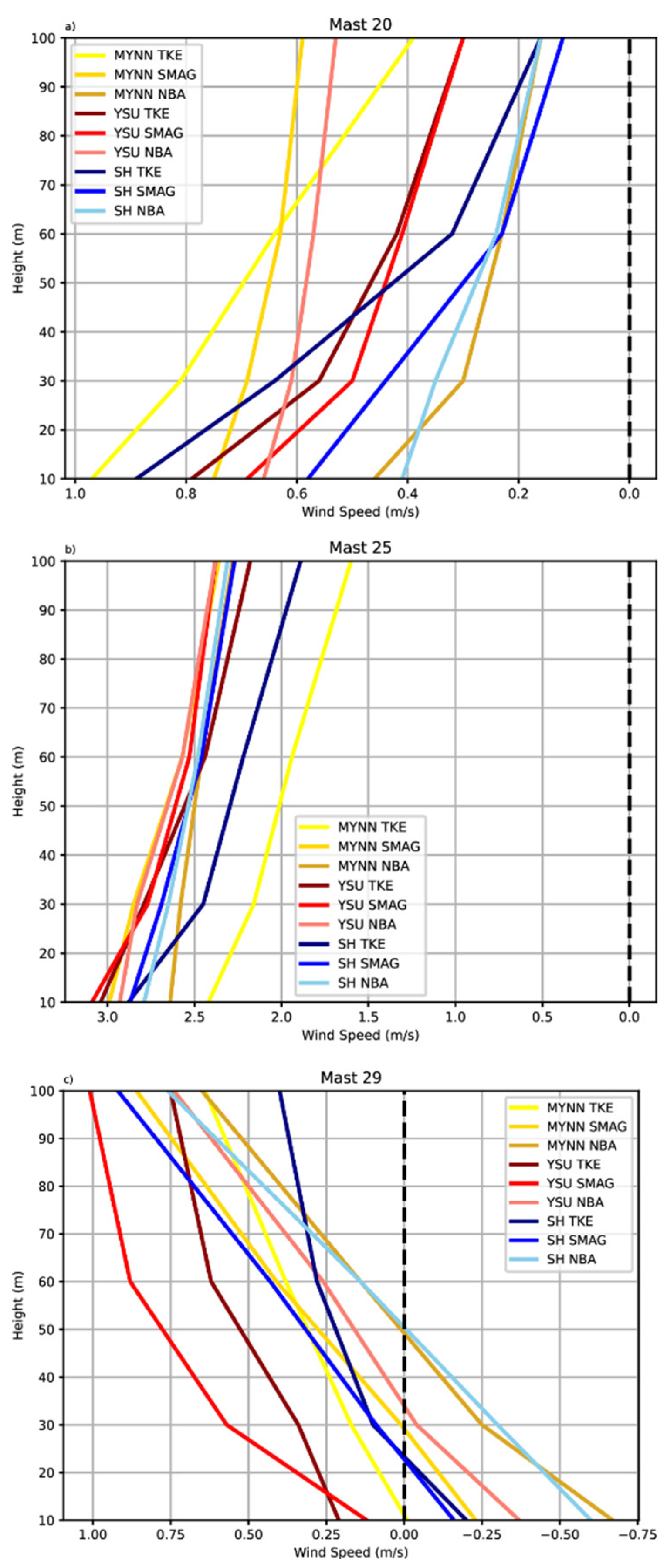
Figure 13.
Daily Diurnal wind speed at 100m of (a) Northeastern flow at Mast 20 (b) Southwestern flow at Mast 20 c) Northeastern flow at Mast25 d) Southwestern flow at Mast 25 e) Northeastern flow at Mast 29 f) Southwestern flow at Mast 29. Box plots include the entire time period of the study.
Figure 13.
Daily Diurnal wind speed at 100m of (a) Northeastern flow at Mast 20 (b) Southwestern flow at Mast 20 c) Northeastern flow at Mast25 d) Southwestern flow at Mast 25 e) Northeastern flow at Mast 29 f) Southwestern flow at Mast 29. Box plots include the entire time period of the study.
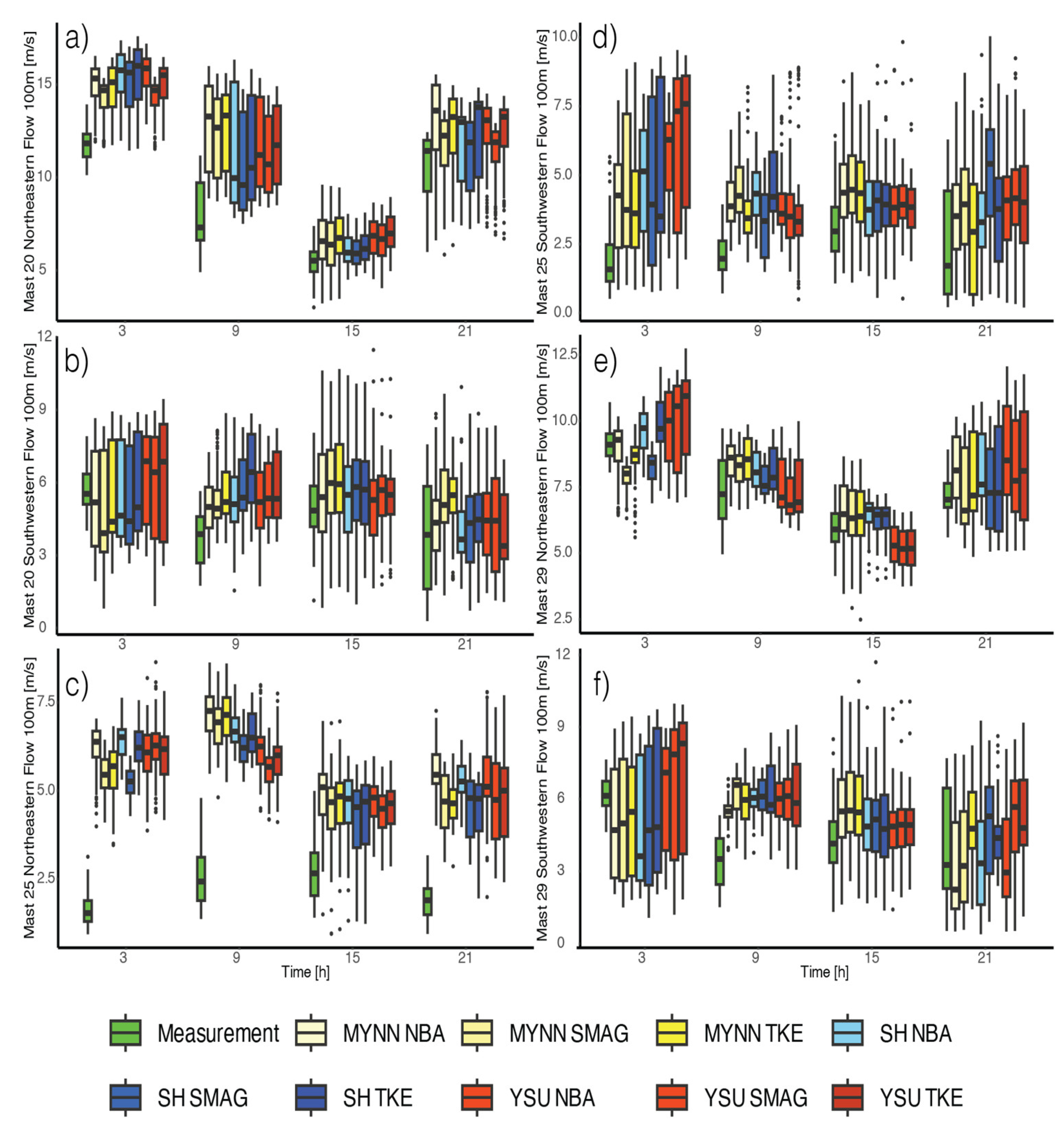
Figure 14.
Comparison of spectra between Mast 20 and WRF-LES d03 Domain(Δx=100m) results for MYNN Parameter and d02 Domain (Δx =1000m).
Figure 14.
Comparison of spectra between Mast 20 and WRF-LES d03 Domain(Δx=100m) results for MYNN Parameter and d02 Domain (Δx =1000m).
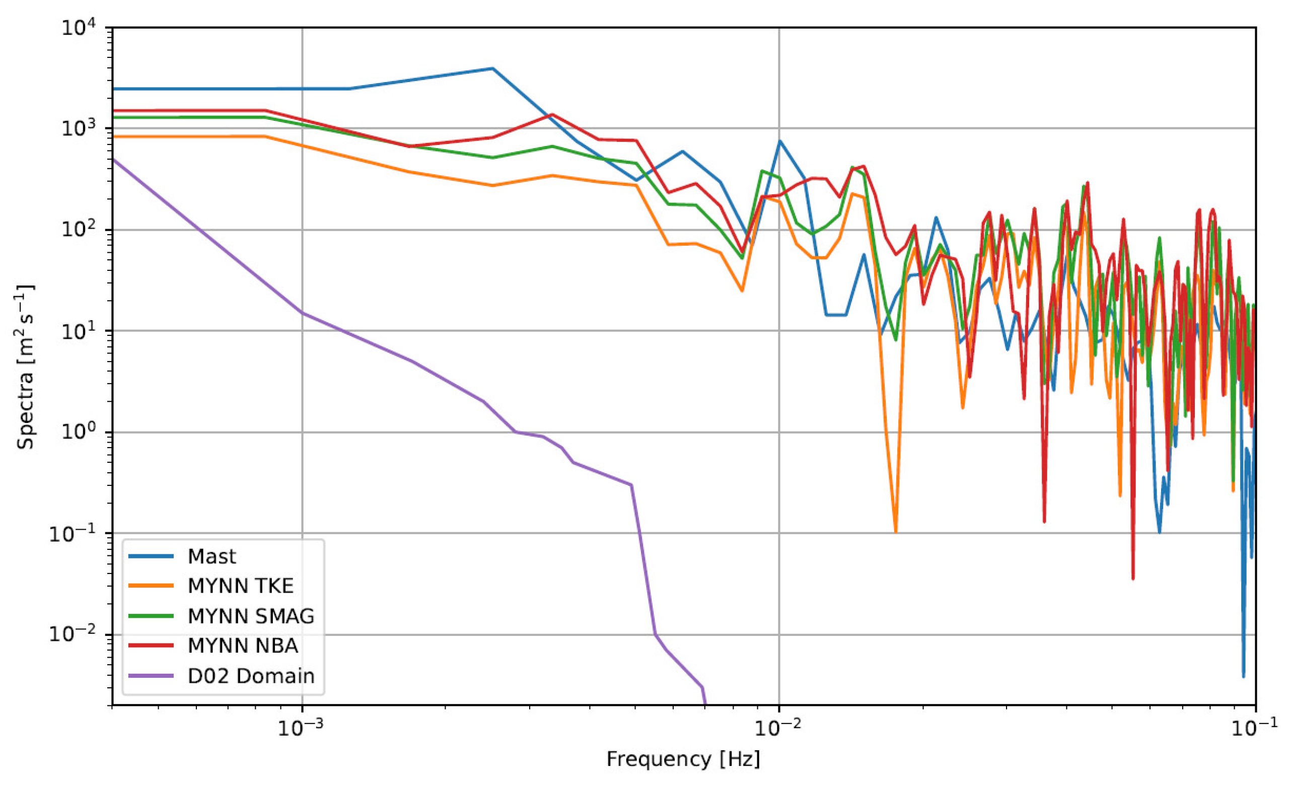
Table 1.
Information on nested simulation domains.
| Domain | Delta X [m] | Nest Ratio | Delta Z [m] | Nx x Ny | Delta t [s] |
|---|---|---|---|---|---|
| d01 | 5000 | - | 50 | 121 x 121 | 5 |
| d02 | 1000 | 5 | 50 | 101 x 101 | 1 |
| d03 | 100 | 10 | 10 | 81 x 81 | 0.2 |
Table 2.
Design of 9 experiment with different PBL and SGS modeling approaches.
| Name |
Mesoscale(d01) 5km |
Mesoscale(d02) 1km | Microscale(d03) 100m |
| MYNN – TKE | MYNN | MYNN | LES (1.5 TKE) |
| MYNN – SMAG | MYNN | MYNN | LES (SMAG) |
| MYNN – NBA | MYNN | MYNN | LES (NBA) |
| SH – TE | SH | SH | LES (1.5 TKE) |
| SH – SMAG | SH | SH | LES (SMAG) |
| SH – NBA | SH | SH | LES (NBA) |
| YSU – TKE | YSU | YSU | LES (1.5 TKE) |
| YSU – SMAG | YSU | YSU | LES (SMAG) |
| YSU – NBA | YSU | YSU | LES (NBA) |
Table 4.
RMSE and Bias results of WRF–LES (simulations) and meteorological tower at 100m.
| Domain | Mast 20 | Mast 25 | ||
|---|---|---|---|---|
| RMSE | Bias | RMSE | Bias | |
| WRF d03 (Δx =100m) WRF d02 (Δx =1000m) |
1.94 | 0.46 | 3.07 | 2.64 |
| 1.96 | 0.52 | 5.47 | 4.95 | |
Disclaimer/Publisher’s Note: The statements, opinions and data contained in all publications are solely those of the individual author(s) and contributor(s) and not of MDPI and/or the editor(s). MDPI and/or the editor(s) disclaim responsibility for any injury to people or property resulting from any ideas, methods, instructions or products referred to in the content. |
© 2025 by the authors. Licensee MDPI, Basel, Switzerland. This article is an open access article distributed under the terms and conditions of the Creative Commons Attribution (CC BY) license (http://creativecommons.org/licenses/by/4.0/).
Copyright: This open access article is published under a Creative Commons CC BY 4.0 license, which permit the free download, distribution, and reuse, provided that the author and preprint are cited in any reuse.


