
Submitted:
10 March 2025
Posted:
11 March 2025
You are already at the latest version
Abstract
The eddy dissipation rate (EDR, or turbulence dissipation rate) is a crucial parameter in the study of the atmospheric boundary layer(ABL). However, existing Doppler lidar-based estimates of EDR seldom offer long-term comparisons that span the entire ABL. Building upon prior research utilizing Doppler lidar wind field data, we optimized the EDR retrieval algorithm using a genetic adaptive approach. The newly developed algorithm demonstrates enhanced accuracy in EDR estimation. The daily evolution of EDR reveals a distinct diurnal pattern in its variation. A detailed four consecutive days study on turbulence generated by Low-Level Jets (LLJ) indicated that EDR driven by heat flux (~10⁻² m²/s³) is significantly stronger than that produced by wind shear (~10⁻³ m²/s³). Subsequently, we examined seasonal variations in EDR at different mixing layer heights (MLH, Zi): elevated EDR values in summer (~7 × 10⁻³ m²/s³ at 0.1Zi) contrasted with reduced levels in winter (~6 × 10⁻⁴ m²/s³ at 0.1Zi). In the early morning, EDR decreases with height for 1 magnitude, while in later stages, it remains relatively stable within 0.1 order of magnitude across 0.1Zi to 0.9Zi. Notably, the EDR during DJF exceeds that of MAM and SON in the afternoon. This suggests that ML turbulence is not solely dependent on surface fluxes (SHF + LHF) but may also be influenced by MLH. A lower MLH (smaller volume), even with reduced surface fluxes, could potentially result in stronger EDR. Finally, we compared the evolution of EDR and MLH in the boundary layer using Doppler lidar data from ARM sites and the PBL Moving Active Profiling System (PBLMAPS) Airborne Doppler Lidar (ADL). The results show that when the ADL is positioned near ARM Southern Great Plains (SGP) sites C1 or E37, the vertical wind data exhibit strong consistency (R = 0.96). The ADL's mobility and flexibility provide significant advantages for future field experiments, particularly in challenging environments such as mountainous or complex terrains. This study not only highlights the potential of utilizing Doppler lidar alone for EDR calculations but also extensively explores the development patterns of EDR within the ABL.
Keywords:
Turbulence dissipation rate (EDR)
; Doppler lidar
; wind speed
; Turbulence
; Genetic Algorithm
; Mixing Boundary layer
; low-level jets (LLJ)
; PBL Moving Active Profiling System (PBLMAPS)
; Airborne Doppler Lidar (ADL)
1. Introduction
The study of turbulence has significant implications across various fields, including astronomy [1], aviation safety [2], optical communication technology [3], laser weaponry [4], wind field retrieval [5], air pollution [6], and oceanography [7]. In astronomy, atmospheric turbulence causes star images observed through telescopes to jitter and flicker, diminishing the quality of observations. Increasing the telescope aperture in ground-based observations does not yield the desired results due to this turbulence. Researchers mitigate these effects by selecting observation sites at high altitudes or locations like Dome in Antarctica, where the atmospheric boundary layer (ABL) is thinner [1]. Similarly, in Free-Space Optical (FSO) communications and laser ranging, atmospheric turbulence-induced refractive index fluctuations affect the coherence of laser beams, leading to optical angle-of-arrival fluctuations, laser beam wander, and scintillation [3]. These phenomena introduce uncertainties and reduce the detection efficiency of these systems, making the study and mitigation of turbulence effects crucial for improving the reliability and performance of optical communication and ranging technologies [3].
Turbulence within the ABL plays a crucial role in transferring heat, momentum, and moisture between the surface and the free atmosphere [8]. This exchange caused by turbulence in the ABL is essential for the accuracy of global and regional atmospheric models [9]. Precise forecasts of ABL are critical for numerous socioeconomic activities, such as pollutant dispersion, air quality forecasting, and the prediction and management of forest fires [10]. TKE production in the ABL primarily occurs at larger scales, typically on the order of the boundary layer height [11]. These large eddies break down into progressively smaller eddies through a process known as the "turbulence energy cascade" in the inertial subrange [12]. Eventually, the scales become sufficiently small for molecular diffusion to dissipate the kinetic energy as heat in the viscous subrange. Current modeling approaches assume that turbulence generation within a grid cell (local production) is counterbalanced by the dissipation of turbulence kinetic energy in the same cell (local dissipation). This local equilibrium assumption is suitable for stationary and homogeneous flow conditions [13], making it applicable at coarser scales [14]. However, at finer resolutions, the basic premises of turbulence closures are violated [15]. Thus, at high horizontal resolutions, the local equilibrium assumption between turbulence generation and dissipation no longer holds: turbulence generated in one grid cell can be transported downwind before it dissipates.
Improved turbulence parameterizations are essential to enhance the accuracy of model results at fine horizontal scales. Yang et al. [16] demonstrated that, in testing the sensitivity of turbine height wind speed to various parameters in the Mellor–Yamada–Nakanishi–Niino (MYNN) planetary boundary layer scheme [17] and the MM5 surface-layer scheme [18] of the Weather Research and Forecasting model [19] in a region with complex terrain, approximately half of the wind speed variance was attributable to the accuracy of the turbulence dissipation rate (or eddy dissipation rate, EDR) parameterization. The EDR also influences the development of several boundary layer processes, including cyclone formation and dissipation [20], the creation of frontal structures [21] and airflow in urban environments and other canopies [22,23]. Thus, accurately representing EDR is vital for improving numerical weather prediction quality. To enhance turbulence parameterizations, it is necessary to study the spatiotemporal variability of EDR in the boundary layer in detail, as well as its dependence on atmospheric stability, terrain features, and turbulence characteristics [24].
Recent advancements in technology have significantly refined the methods for calculating EDR. Traditionally, direct measurements using sonic anemometers and hot-wire anemometry were employed, utilizing the inertial subrange energy spectrum and second-order structure function approaches [25,26]. Peña et al. [26] conducted a study on one-year-long turbulence measurements and modeling using large-eddy simulation domains in the Weather Research and Forecasting model, making numerous comparisons and experimental improvements. However, the meteorological mast was only 250 meters high, limiting its ability to capture boundary layer conditions above 250 meters, which restricted both the comparison with the model and the potential for model improvements. Moreover, these methods are limited by their spatial coverage or/and the necessity for high-frequency data acquisition systems.
The advent of remote sensing technologies, particularly Doppler Lidar and radar wind profilers [27], has greatly enhanced the capability to study EDR. It provides three-dimensional wind data over larger spatial scales and extended time periods, enabling comprehensive turbulence studies. The methodologies to derive EDR include the Doppler spectra width [28], line-of-sight velocity spectrum [27], longitudinal structure function [29], and azimuthal structure function [30]. Furthermore, Doppler Lidar's ability to provide detailed turbulence measurements at various altitudes and its deployment flexibility in complex terrains make it a superior tool for turbulence research compared to traditional in-situ instruments [31,32].
EDR estimation must be conducted within the inertial subrange, and due to lidar signal-to-noise ratio (SNR) limitations beyond the ABL, it is necessary to analyze EDR in conjunction with mixing boundary layer height (MLH). The effectiveness of Doppler lidar depends on atmospheric backscatter intensity. While typical atmospheric conditions provide sufficient backscatter strength, lidar measurements become unreliable under low aerosol concentrations within the ABL (or outside the ABL), as well as during rain or fog [27]. Additionally, in many cases, the atmosphere fails to meet the inertial subrange conditions, leading to larger EDR estimation errors. These challenges emphasize the need for accurate MLH determination to properly define the scope of EDR estimates. Rajput et al. [33] used 1290 MHz radar wind profiler data to calculate MLH and EDR over a central Himalayan site from November 2011 to March 2012, providing monthly mean diurnal variations of turbulence parameters with height. While existing studies report the spatiotemporal distribution of EDR [27,30,34,35], most are limited to short-term field experiments and lack long-term (annual) observations of EDR distribution across the entire ABL. The Atmospheric Radiation Measurement (ARM) Southern Great Plains (SGP) site offers a valuable opportunity for multi-year Doppler lidar data [36,37]., enabling extended research on EDR variability.
Based on the research above, this paper compares optimized the EDR retrieval algorithm based on the Fast Fourier Transfer (FFT) method. The second section presents the Doppler lidar observational datasets, detailing the retrieval algorithm for MLH and describing the computational methodology for EDR estimation. Section three focuses on further introducing an optimized algorithmic approach utilizing genetic algorithm-based frequency range selection. The fourth section presents a comprehensive analysis of four consecutive days of EDR measurements, including a detailed case study of Low-Level Jet (LLJ) phenomena. Furthermore, we systematically investigate the vertical EDR profiles across different seasons, focusing on their evolution through various stages of ABL development. Section five performs a comparative analysis of mobile Doppler lidar measurements from SOMAS (School of Marine and Atmospheric Sciences, Stony Brook University) against stationary lidar measurements obtained from the ARM C1 and E37 sites. The final section presents the conclusion and discussion.
2. Data and Methods
The ARM SGP site is equipped with an extensive array of meteorological observation instruments, making it a valuable resource for atmospheric research. Among its various facilities, the C1 site is particularly notable for its comprehensive suite of instruments. In this study, we primarily utilize Doppler Lidar data and radiosonde data.
2.1. Data and Mixing Layer Height
At the ARM SGP C1 site, the Doppler lidar delivers high-resolution three-dimensional wind field data, which is vital for calculating turbulence dissipation rates and understanding the vertical structure of the atmosphere. Complementing this, radiosondes provide essential vertical profiles of temperature, humidity, and pressure [36,37]. The specific parameters and configurations of the instruments used in this study are detailed in Table 1. It should be noted that the SGP Doppler lidar has a vertical wind, resolution of 1-3s, but a horizontal wind speed resolution of 3-6 mins.
The PBL (Planetary Boundary Layer )Moving Active Profiling System (PBLMAPS) at Stony Brook University utilizes a low-roof, four-wheel-drive Ford Transit cargo van as its mobile platform. A single-beam Airborne Doppler Lidar (ADL) is mounted on the van's roof near the optical window to provide collocated vertical velocity measurements. Space is reserved for future installation of additional ADL beams to enable horizontal wind measurements. Data collection was conducted from September 28 to October 2, 2023. In this study, data collected using PBLMAPS positioned near the E37 site on September 30, 2023, and the C1 site on September 28, 2023, were analyzed(relative positions in Figure 1).
The parameters of the Doppler lidars from both the ARM and PBLMAPS systems are detailed in Table 1. The ADL is designed to accommodate a wide range of platform and atmospheric conditions, providing greater flexibility. To support aircraft speeds of 50–160 m/s and ground-relative atmospheric wind speeds of ±80 m/s, the data system requires a bandwidth of 30-300 MHz and a sampling rate of 1 G/s. The range gates are adjustable from 18 to 90 meters, with the option for selectable gate overlaps. Please note that ADL currently lacks horizontal wind field measurements. Therefore, the EDR calculations for the ADL were performed using horizontal wind speed data provided by nearby C1 or E37 sites. Since PBLMAPS has reserved space for horizontal wind field measurements, it will be able to get horizontal wind in later 2025. Additionally, to verify the accuracy of the Doppler lidar measurements, wind field data from the radiosonde at the C1 site was utilized, as detailed in Table 1.
This study uses the method of Chu et al. [38] to determine MLH from Doppler Lidar data. The algorithm first utilizes wavelet analysis to identify whether the day is dominated by large-scale turbulence eddies. Subsequently, wavelet analysis is applied across all heights to construct a 2-D vertical velocity variance by selecting the power spectrum within a specific frequency range that corresponds to the dominant eddy size. Finally, dynamic thresholds are employed to reconstruct the 2-D variance profile, thereby determining the MLH. This algorithm effectively addresses challenges related to varying sizes of turbulent eddies and gravity waves in velocity variance calculations, as well as the limitations of fixed variance threshold methods.
2.2. Calculation Eddy Dissipation Rate from Doppler Lidar
In boundary-layer meteorology, the quantification of turbulence from measured data is often based on the assumption of homogeneity and local isotropy in the small scales of turbulence, which has been found to be valid in high Reynolds number flows [12]. Under these assumptions, the energy cascade of eddies from larger to smaller scales in the inertial subrange of turbulence can be described by a model [27,33] for the energy spectral density S(k):
where k is the wave number, is the TKE EDR, and α is a universal constant (0.55). Integration of the energy spectrum yields the variance :
where , L=NU=U/f. Therefore, the EDR [39] can be inferred from Formula 2:
which, , if not removed, would induce an overestimation of . So, we use instead of . Then we can get:
where , and the B is the bandwidth, equivalent to twice the Nyquist velocity, and is the signal spectral width (1.5 m/s). We can get these parameters from Table 1. L1 is the shortest time interval multiplied by the horizontal wind speed, and LN is the selected time multiplied by the wind speed. In this study, we selected 4 minutes (240 seconds). Assuming a horizontal wind speed of 5 m/s, L1 is 5 meters and LN is 1200 meters. This method assumes that both length scales L1 and LN lie within the inertial subrange. Consequently, the selection of the sample size N must be meticulously considered to ensure that only turbulence contributions within the inertial subrange are included in the calculations.
Using the equations provided above, we can calculate the EDR as described data in Section 2.1. By applying FFT to the wind field data, we can estimate the EDR using Equation 1. Additionally, with the vertical and horizontal wind field data from the Doppler lidar, we can estimate the EDR using Equation 4. To verify the accuracy of the EDR estimation, we can calculate the Lidar error using Equation 5 and determine the fraction error according to the method proposed by Bodini et al. [39]. For more details on error analysis, please refer to the relevant literature [33,34,35,39].
2.3. Calculation Eddy Dissipation Rate from Radiosonde
At the ARM SGP C1 site, four radiosondes are emitted each day. The ascent rate of the radiosondes used in this study was roughly 5m/s. They had a temporal resolution of 1 s corresponding to a 5m height resolution (roughly, not strictly accurate). The commonly used method to calculate turbulent dissipation rate from radiosonde data involves converting pressure and temperature information into potential temperature, which is a complex process. Additionally, rearranging potential temperature in ascending order to derive the turbulent dissipation rate is cumbersome and prone to errors [40]. To address these drawbacks and reduce computational complexity, this paper employs a method like that described in Section 2.2, as outlined in Equation 1. EDR is calculated using radiosonde data collected around noon, specifically at 11:30 (UTC-6). This approach estimates the EDR over approximately 160 seconds within the ABL, covering altitudes from 200m to 800m.
3. Estimate EDR Using Doppler Lidar
Using the data and algorithms outlined in Section 2, we first compare the results derived from Doppler lidar and radiosonde measurements. Next, we conduct comparisons inside and outside the boundary layer. Subsequently, we propose a novel EDR retrieval algorithm that utilizes a genetic algorithm to optimize the selection of frequency ranges.
3.1. Comparison of FFT Between Lidar and Sonde
To ensure the comparability of wind field data between radiosonde and Doppler lidar, this study selects radiosonde wind field data between 0.2 km and 1 km. We selected vertical wind field data from Doppler lidar at 0.285 km, 0.495 km, and 0.705 km between 11:00 and 12:00 (UTC-6). FFT was performed on these data, and the results are shown in Figure 2. The FFT spectra for Doppler lidar at altitudes of 0.285 km, 0.495 km, and 0.705 km are very similar. Due to the radiosonde's limited observation time of less than 100 seconds, the minimum frequency is greater than 10-2Hz. this study uses Equation 1 (0.01hz to 0.1 Hz) from Section 2.2 to fit the FFTs at the three altitudes, the EDR at 0.285 km, 0.495 km, and 0.705 km are 0.51 m²/s³, 0.42 m²/s³, and 0.70 m²/s³, respectively. The EDR from the radiosonde (200m to 800m) is ~1.1 m²/s³. The results indicate that the EDR derived from radiosonde measurements and Doppler lidar at various heights falls within the same order of magnitude, though it also reflects the heterogeneity of turbulence. While the EDR averaged across three heights from lidar data and the EDR obtained from radiosonde measurements differ by less than one order of magnitude, the relative error can reach up to 50%.
The next step will involve further comparison with meteorological tower data. However, this work has not yet been carried out due to the unavailability of meteorological tower data from the ARM SGP C1 site. Nevertheless, numerous studies have already compared meteorological tower data with Doppler lidar-derived EDR calculations, demonstrating that these methods are sufficient for estimating EDR and observing relative changes in the boundary layer [30,31,34,35]. Therefore, this does not affect the general applicability of the results presented in this paper.
3.2. Comparison of Eddy Dissipation Rates Inside and Outside the Boundary Layer
To compare the relative accuracy of EDR, we selected data for half an hour before and after 9:00 AM and 2:00 PM (UTC-6) at three different altitudes: 0.195 km, 0.5855 km, and 1.425 km. At 2:00 PM, all three altitudes were within the boundary layer. At 9:00 AM, 0.195 km was within the boundary layer, 1.425 km was outside the boundary layer, and 0.586 km transitioned from outside the boundary layer to within the boundary layer. The FFT spectra at 9:00 AM are shown in Figure 2a, and the FFT spectra at 2:00 PM are shown in Figure 2b. Figure 2c presents the vertical wind field data, where the red lines represent data at the three different altitudes around 9:00 AM, and the black lines represent data at the three different altitudes around 2:00 PM. By comparing Figure 2a, we observe that at the height of 1.425 km, the FFT power spectrum does not exhibit a -5/3 slope from 0.01Hz to 0.1 Hz, indicating the absence of turbulence at this altitude around 9:00 AM. However, at 0.195 km and 0.5855 km, both show a -5/3 slope from 0.01Hz to 0.1 Hz, indicating the presence of turbulence at these altitudes around 14:00. The turbulence intensity at 0.195 km is greater than at 0.586 km. By comparing Figure 2b, we find that the turbulence intensities at all three altitudes are nearly identical, with the 0.586 km (yellow) being slightly stronger.
To verify the accuracy of the above FFT results and to provide a more intuitive representation of turbulence characteristics, this paper uses Equation 1 from Section 2.2 to fit the FFTs at the three altitudes for both time periods. The turbulent dissipation rates were then derived from the fitting results. At 9:00 AM, the estimated EDR (ε) are as follows: 1.37 ×10⁻¹ m²/s³ at 0.195 km, 3.6×10⁻³ m²/s³ at 0.586 km, and 3.7×10⁻⁹ m²/s³ at 1.425 km. At 14:00, the estimated EDR (ε) are: 3.7×10⁻² m²/s³ at 0.195 km, 6.8×10⁻² m²/s³ at 0.5855 km, and 6.5×10⁻³ m²/s³ at 1.425 km. The turbulence intensity mentioned above is consistent with the FFT results shown in Figure 3a and 3b.
Figure 3 shows a significant difference in EDR inside and outside the boundary layer. The data indicates that at the bottom of the boundary layer (0.195 km), the EDR (ε) at 9:00 AM (1.37 10-1 m²/s³) is stronger than at 2:00 PM (3.7 10-2m²/s³). However, at 0.586 km, the EDR at 2:00 PM (6.8x10⁻²m²/s³) is slightly stronger than at 9:00 AM (3.6 ×10⁻³ m²/s³). At 1.425 km, the EDR at 14:00 (6.5x10⁻²m²/s³) is significantly stronger than at 9:00 (3.6 ×10-²/s³). Additionally, it is observed that at 9:00 AM, turbulence develops gradually from the bottom upward. In contrast, at 2:00 PM, the turbulence intensities at the three different altitudes are similar and of the same order of magnitude. The EDR results calculated using Equation 4 from Section 2.2 are consistent with those obtained from the FFT method. For instance, within a ±30-minute window around 14:00, the EDR computed using Equation 4 (with variance calculated over 2 minutes) yields a median value of approximately 1 ×10⁻² m²/s³ at a height of 585 m, which is higher than the value of 5×10⁻⁴m²/s³ observed around 09:00.
However, it is important to note that, the layer at 1.425 km is located higher than MLH at 09:00. The turbulence in free atmosphere is derived from larger scales than that in mixing layer (ML), making it difficult to locate the inertial subrange for the FFT in the desired same frequency range in ML . Equation 4 is derived from Equation 1 and therefore exhibits similar issue. Therefore, the EDR above the MLH will be excluded in this study. To address this, it is crucial to know the height of the ABL top, or MLH, to accurately identify these conditions.
3.3. Using the Improved Method to Obtain EDR
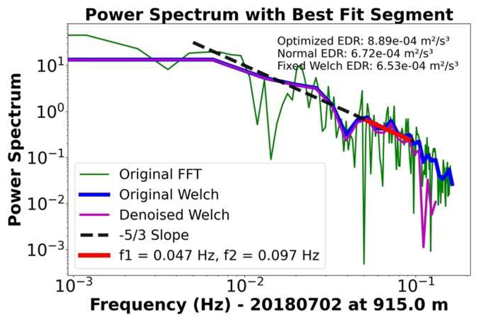
When turbulence driven by flux is superimposed on large-scale ABL movements, the algorithm described in Section 2.2 becomes inapplicable, even within the ABL. As shown in Figure 3b, the FFT of the vertical wind at various heights within the boundary layer adheres to a -5/3 slope. However, Figure 5 reveals that between 12:00 and 13:00 (UTC-6) at an altitude of 915 meters, the FFT of the vertical wind field no longer conforms to this -5/3 slope from 0.1 Hz to 0.01 Hz. Directly applying the default FFT method to fit data from 0.1 Hz to 0.01 Hz would physically be inaccurate. To address this challenge, we propose a novel algorithm that builds upon denoising techniques and incorporates an adaptive approach based on genetic algorithms to identify the frequency range that aligns with the expected slope.
The core idea of the algorithm is to adaptively find the frequency range that satisfies the -5/3 slope, followed by fitting to obtain the EDR. We leverage the advantages of the Welch FFT method, particularly its reduced spectral leakage characteristics. The Welch FFT employs window functions to effectively mitigate spectral leakage, thereby ensuring a more concentrated spectral power distribution at the signal's actual frequency components. The methodological workflow, as illustrated in Figure 4, comprises the following detailed steps:
- Select Data: Choose 30 minutes of vertical wind field data at a specific altitude.
- FFT Processing: Perform a FFT using the Welch FFT method with a window size of 50.
- Denoising: Denoise the spectrum by averaging the 10 highest frequency points. This step is critical as noise near the 0.1 Hz end could otherwise skew the results, especially in scenarios where low-frequency signals are obscured by background noise.
- Adaptive Fitting: Finally, employ an adaptive fitting approach using genetic algorithms to pinpoint the frequency range that yields the minimal fitting error. This method allows for dynamic adjustment to identify the most suitable frequency range for the -5/3 slope, enhancing the robustness and accuracy of the EDR calculation. Genetic algorithms are optimization techniques inspired by natural selection processes, utilizing operations such as selection, crossover, and mutation to evolve solutions to complex problems [41,42]. This paper employs genetic algorithms to identify the optimal frequency range that minimizes the mean absolute error (MAE) of the -5/3 slope in the FFT frequency spectrum.
- Repeat the Process: Repeat these steps for all heights and time intervals to ensure comprehensive data analysis.
The improved algorithm can effectively address the limitations of the algorithm described in Section 2.2. As shown in Figure 5, the FFT Power Spectral Density (PSD) at approximately 13:00 on July 2, 2018, at a height of 915 meters (within ABL) is presented. In the figure, the green line represents the original FFT PSD, the blue line shows the original Welch PSD, the magenta line indicates the denoised Welch PSD, and the red line marks the frequency range identified by the adaptive algorithm. When using the standard FFT (green line in Figure 5) to calculate the EDR based on Equation (1) within the fixed frequency range of 0.01-0.1 Hz, the resulting EDR is 6.72×10⁻⁴m²/s³. When using the Welch FFT (blue line in Figure 5) within the same fixed frequency range, the calculated EDR is 7.53 ×10⁻⁴ m²/s³. However, when applying the Welch FFT combined with the adaptive algorithm to determine the frequency range (red line in Figure 5), the resulting EDR is 1.05 ×10⁻³ m²/s³. From Figure 5, it is evident that only the frequency range marked in red satisfies the conditions of the inertial subrange (with a slope of -5/3). The differences in EDR values further corroborate this observation. This demonstrates that the adaptive algorithm significantly improves the accuracy of EDR calculations by identifying the appropriate frequency range that aligns with the inertial subrange characteristics.
Although the adaptive fitting method utilizing a genetic algorithm can provide the most accurate results, it demands substantial computational resources. When computational resources are limited, the fixed Welch method (fixed 0.01Hz to 0.1Hz) can serve as a viable alternative. In cases where horizontal wind speed data is available and computational resources are constrained, the results from Section 2.2 may also be considered as an alternative option.
Figure 5.
The FFT power spectrum and the improved EDR Algorithm Results.
4. Statistical Analysis of EDR Results
4.1. Daily Evolution of Eddy Dissipation Rate with MLH
To compare the effectiveness of the methods between Equation 4 and the FFT fitting approach, this paper calculates the EDR for the entire day of May 17, 2018, using Equation 4. The MLH calculated using the method from Section 2.1 is also utilized, represented by the blue or red points in Figure 6.
From Figure 6 (where EDR is calculated using Equation 4), it can be seen that the EDR within the ML is of the same order of magnitude and similar to the results obtained in Section 3.1 (using Equation 1). The average EDR values between 11:00 and 12:00 at the heights of 0.285 km, 0.495 km, and 0.705 km were found to be 0.0563 m²/s³, 0.0317m²/s³, and 0.0321 m²/s³, respectively. These values are of the same order of magnitude and exhibit a similar relative trend as the values (0.04-0.07 m²/s³) presented in Section 3.1. Given that all the heights are within the boundary layer (below MLH), the average EDR values are also of the same order of magnitude as those observed at 14:00. This result suggests that the EDR calculation based on Equation 4 is reliable and suitable for estimating relative EDR magnitudes within the boundary layer, particularly under conditions with limited computational resources and moderate precision requirements.
Figure 6 highlights intriguing phenomena within the convective boundary layer (CBL). While the EDR within the CBL exhibits overall variation, it fluctuates consistently within the range of 10⁻³ to 10⁻¹ m²/s³. At night, the EDR in the PBL can be exceptionally low, with values at 500 meters dropping below 10⁻⁶ m²/s³. Note that EDR obtained from the variance of vertical velocity data in this test is not physically meaningful, as turbulence is nearly absent in this case.
Nighttime EDR generally remains below 10⁻⁴ m²/s³; however, between 05:00 and 06:00, EDR at altitudes of 0.5–1.2 km increases to approximately 10⁻³ m²/s³, suggesting notable turbulence during this period. This is supported by the low fractional error in this region, as shown in Figure 6d. However, the fractional error associated with the increased EDR near the PBL top is relatively high, making it less reliable than this area. Figure 6e shows that the gravity wave is connected to the surface at the bottom and to the capping inversion at the top. A closer examination of Figure 6c reveals that while the top of this EDR structure connects to the capping inversion, the bottom does not connect to the surface. Additionally, the near-surface EDR between 02:00 and 04:00 is significantly lower than that near the surface between 20:00 and 24:00. The strengthening of EDR at this time may be due to meteorological factors such as clouds or residual layers, which warrant further study. These phenomena suggest that although there is no flux-driven turbulence at night, other mechanisms such as low-level jets (LLJs), gravity waves, or wind shear may generate turbulence.
From the above, we can see that the EDR and MLH reveal many interesting phenomena. However, this observation is based on a single day. To further summarize and generalize the boundary layer evolution, we need to compare the boundary layer evolution over multiple days.
4.2. EDR Evolution in the Presence of Lower Lever Jet
LLJs are narrow bands of strong winds occurring within the lower part of the atmosphere, typically between 100 and 1000 meters above the ground [8]. These jets are often formed due to the interaction between diurnal thermal variations and topographical features, leading to significant wind speed maxima during the night. LLJs play a crucial role in various meteorological phenomena, including the transport of moisture and pollutants, as well as the initiation and sustenance of convection. EDR is a critical factor in understanding and predicting the behavior of LLJs. High EDR values indicate intense turbulent mixing, which can disrupt the coherence of the jet and influence its strength and persistence. Conversely, lower EDR values suggest more stable conditions that allow the jet to maintain its structure [34]. Accurate estimation of EDR, therefore, is essential for modeling the dynamics of LLJs, particularly in predicting wind energy potential, pollutant dispersion, and weather forecasting.
EDR can enhance the detailed description of the LLJ process. As shown in Figure 7, we selected four consecutive days, with the nights of April 16-17, 2023, lacking an LLJ, and the subsequent nights of April 17-18, 2023, featuring an LLJ. Since turbulence at this point is driven not only by flux but also by wind shear (LLJ), we employ the optimized algorithm from Section 3.4 to estimate the EDR for improved accuracy. Figure 7a presents the vertical wind field data, Figure 7b shows the variance of the vertical wind field, Figure 7c displays the EDR, Figure 7d illustrates the horizontal wind speed, and Figure 7e depicts the horizontal wind direction. The circles in the figures represent the MLHs.
The EDR driven by heat flux during the day is significantly greater than the EDR driven by wind shear (LLJ). Figure 7 shows the transition from nights without a LLJ to consecutive nights with the presence of an LLJ. From Figure 7c, we can observe that during the first night (April 16-17), there was no turbulence or LLJ, while during the second night, both turbulence and the LLJ were weak (EDR: ~ 5×10⁻³ m²/s³). On the third night, both turbulence and the LLJ strengthened (EDR: ~ 10⁻² m²/s³). A similar pattern is observed in the vertical variance in Figure 7b. Additionally, the EDR driven by heat flux during the day (~10⁻² m²/s³) is significantly greater than the EDR driven by wind shear (LLJ) at night (~10⁻3 m²/s³). The variation in EDR driven by the LLJ at night is relatively small, while the EDR driven by heat flux during the day shows much larger fluctuations. For instance, the daytime variation on April 16 is about 3-4 orders of magnitude (EDR between 10⁻⁴ and 10⁻¹ m²/s³), whereas the nighttime variation from April 16 to 17 is around 1 order of magnitude (EDR between 10⁻3 and 10⁻2 m²/s³).
Due to the influence of the LLJ, not only does the LLJ develop at night, but it also significantly impacts boundary layer development during the day. In the morning, when the boundary layer begins to rise, turbulence is easily generated by windshear, which in turn influences the boundary layer's development. For example, around 09:00 (UTC-6) on April 17, we can clearly see a noticeable jump in the MLH, which is mirrored by a similar jump in EDR (Figure 7c) at the same time (around 800m). Observing Figure 7d, we notice that at this moment, the horizontal wind speed near the surface is less than 10 m/s, but the ABL top (MLH) corresponds to a wind speed close to 20 m/s, indicative of a typical LLJ structure. At this point, the MLH jumps directly from near the surface to around 800 meters. Additionally, between 10:00 and 11:00 on April 18, 2023, clear gravity waves are observed, including both updrafts and downdrafts. After the gravity waves, the ABL continues to develop slowly. On the morning of April 19, between 10:00 and 11:00, a distinct updraft is visible, primarily originating from the top of the ABL. Due to the persistent updraft, the MLH rapidly develops from 1.0 km to 1.5 km. The development of the ABL on April 16 follows a typical pattern, but on April 19, due to the influence of the LLJ, the LLJ not only develops at night but also has a significant impact on the ABL development during the day.
Although three nights feature LLJs, their generation and evolution have distinct characteristics, with the EDR on the third night being significantly stronger than on the second night. On the night of April 16-17, the EDR initially decreases to 10⁻⁵ m²/s³ after sunset, and the height drops to the ground. On the night of April 17-18, the EDR gradually decreases to 10⁻4 to 10⁻3 m²/s³ after 18:00, with this value sustained between the surface and 800 meters. After 01:00, the EDR increases to 10⁻³ m²/s³, with this value maintained between 0 and 500 meters. The EDR during the night of April 18 to 19 (~10⁻2 m²/s³) is stronger than the LLJ from the night of April 17 to 18 (~10⁻3 m²/s³).
4.3. Variation of EDR with Altitude in Different Seasons at Different Boundary Layer Development Stages
To investigate whether EDR exhibits a distinct seasonal cycle, we analyzed median EDR values at six different heights (0.1Zi, 0.2Zi, 0.3Zi, 0.4Zi, 0.7Zi, and 0.9Zi) from 2016 to 2023 at the ARM SGP C1 site. To assess the variation across the four quarters, we further looked for median EDRs by season. Additionally, to compare EDR behavior during different phases of boundary layer development, we examined its evolution from sunrise to sunset at four representative stage fractions (0.1, 0.3, 0.5, and 0.7), as shown in Figure 8a–d. The EDR at this section is derived from the genetic algorithm-based optimization algorithm presented in Section 3.3.
From Figure 8, it is evident that the median EDR variations with height differ across different boundary layer development stages. At the early stage after sunrise (Figure 8a), the median EDR exhibits a consistent decrease with height across all four seasons. At the near-surface level (0.1Zi), DJF (~3 × 10⁻⁴ m²/s³) is significantly lower than MAM (~1.2 × 10⁻³ m²/s³) and JJA (~1.5 × 10⁻³ m²/s³). Between 0.1Zi and 0.3Zi, the median EDR remains nearly constant, but from 0.5Zi onward, it decreases sharply. The most pronounced drop occurs in summer, where the median EDR declines by one orders of magnitude, from ~1.5 × 10⁻³ m²/s³ at 0.1Zi to ~1.1 × 10⁻4 m²/s³ at 0.9Zi. This pattern suggests that during the initial stage of boundary layer development, turbulence-driven ML gradually extends upward, while turbulent mixing within the ML remains inhomogeneous, exhibiting a weakening trend from the surface upward.
After the median EDR is fully developed within the ABL, the EDR inside the ABL remains relatively consistent. Further comparisons (Figure 8b–d) reveal that after a period of boundary layer development, the median EDR remains nearly constant between 0.1Zi and 0.9Zi, with fluctuations within approximately 0.1 order of magnitude. For instance, after sunrise at 0.3Zi (Figure 8b), the median EDR stabilizes at ~2 × 10⁻³ m²/s³ in autumn (SON) and winter (DJF), while it remains around ~3 × 10⁻³ m²/s³ in spring (MAM) and around ~5 × 10⁻³ m²/s³ in summer (JJA). In Figure 8c, the largest seasonal difference occurs in JJA, where the median EDR varies from ~4 × 10⁻³ m²/s³ at 0.1Zi to ~7 × 10⁻3 m²/s³ at 0.9Zi, representing a difference of 0.3 orders of magnitude. Compared to the one-order magnitude difference observed in Figure 8a, this indicates a more uniform median EDR distribution at later stages of boundary layer development (Figure 8b–d), which is consistent with turbulence-driven boundary layer growth theory.
The development of the median EDR exhibits distinct characteristics across different seasons. As shown in Figure 8c, summer (JJA) exhibits significantly higher median EDR values (~6.8 × 10⁻³ m²/s³) compared to other seasons. This result is consistent with the findings of Bodini et al. [35], although their analysis was limited to fixed altitudes and did not include comparisons across different heights. Additionally, at the 0.7 stage after sunrise, the median EDR begins to decrease across all four seasons, indicating that the median EDR weakens in the later afternoon. Notably, DJF initially exhibits the lowest median EDR values (~3.8 × 10⁻⁴ m²/s³ in Figure 8a), but subsequently shows a gradual increase. At the 0.3 stage (Figure 8b), DJF EDR almost catches up with SON (~2 × 10⁻³ m²/s³), and by the 0.5 stage (Figure 8c), DJF surpasses SON (~1.7 × 10⁻³ m²/s³ vs. ~1.1 × 10⁻³ m²/s³, respectively). At the 0.7 stage (Figure 8d), DJF EDR further exceeds MAM (~1.5 × 10⁻³ m²/s³). This trend suggests that EDR within the ML in DJF continues to develop, despite lower temperatures, and does not remain weaker than in spring or autumn. This phenomenon may be attributed to the lower MLH during DJF, where a comparable level of heat flux is concentrated within a reduced vertical extent, thereby enhancing EDR generation. Even with diminished surface fluxes, a lower MLH (smaller volume) can contribute to stronger EDR. Furthermore, the observed pattern remains consistent across different EDR algorithms, as demonstrated by the similar results from both Formula 4 and the enhanced algorithm detailed in Section 3.3. Due to space constraints, EDR results from Formula 4 are not presented in the manuscript.
The above analysis provides insights into EDR behavior across different stages of ABL development, revealing several meaningful phenomena. However, it is also important to acknowledge the limitations of this study. For instance, data near the boundary layer top (~Zi) is excluded due to the significant deterioration of the Doppler lidar signal-to-noise ratio (SNR) at these altitudes, which affects measurement reliability. Additionally, as the ABL rapidly dissipates near sunset, further investigation is required to examine this stage in greater detail to improve our understanding of turbulence evolution during this transition period.
5. Comparison of EDR Between Airborne Doppler Lidar and ARM SGP Doppler Lidar
5.1. Comparison of Vertical Wind Fields Between ADL and SGP Sites
To further leverage the advantages of Doppler Lidar-derived EDR in analyzing ABL development, we compared the data obtained by our research group's mobile compact airborne Doppler Lidar (ADL) with that from the ARM site’s Doppler Lidar at C1 (2023-09-30) and E37 (2023-09-28). The results are shown in Figure 9. The three panels of Figure 9a-c display the vertical wind field data obtained on 2023-09-28 from the ARM site’s C1 (top), E37 (bottom), and ADL (middle), with the ADL deployed ~1 meter away from the C1 site. We observed that the vertical wind field data from the ADL and C1 were nearly identical, while there was a significant difference with the E37 site. The three panels of Figure 9d-f show the vertical wind field data obtained on 2023-09-30 from the ARM site’s C1 (top), E37 (bottom), and ADL (middle), with the ADL deployed ~2 meters away from the E37 site. Similarly, we found that the ADL data was nearly identical to that from the E37 site, but there was a significant difference with C1.
To further validate the consistency between the ADL and SGP site vertical wind field data, we compared the data from the C1 site and ADL on September 28th. To minimize errors due to clock differences, the vertical wind field data were averaged every 30 seconds at different heights (30m intervals) within the boundary layer (using the MLH calculated in Section 2). After grouping the ADL and C1 site data according to the above method and comparing them, the results showed a high correlation: a correlation coefficient (R) of 0.964. Note that during this time, the ADL was deployed next to the C1 site. The same comparison was then performed between the E37 site and ADL on September 30th, resulting in an R value of 0.968, with the ADL deployed next to the E37 site. These results indicate a high level of consistency between the two datasets, demonstrating that the ADL can accurately capture vertical wind field results consistent with those of the C1 and E37 sites.
However, when comparing the ADL data with that of the C1 or E37 sites without co-location, using the same method on the same day, the R value was less than 0.1, demonstrating the spatial and temporal differences between the C1 and E37 sites (a direct comparison between the ARM sites C1 and E37 also yielded similar results). This shows significant spatial variability between different ARM sites
5.2. Comparison of EDR Between ADL and SGP Sites
After validating the consistency of the vertical wind field data between the ADL and SGP sites. To leverage the high temporal resolution of the Doppler lidar, we employ Equation 4 from Section 2.2 to retrieve the EDR in this section. Since the ADL was not in scanning mode and did not capture horizontal wind field data, the horizontal wind speed was entirely sourced from the ARM site. Figure 10a-c shows the comparison of EDR results obtained by the SGP sites C1, E37, and the ADL when deployed at the C1 site. Figure 10d-f shows the comparison of EDR results when the ADL was deployed at the E37 site.
From Figure 10a-c, we can see that the EDR from the ADL is nearly identical to that from C1. Figure 10a displays the EDR calculated from the vertical and horizontal wind field data obtained by the Doppler lidar at the C1 site; Figure 10b shows the EDR calculated using the vertical wind field data obtained by the ADL and the horizontal wind field data from the SGP C1 site; Figure 10c shows the EDR calculated from the vertical and horizontal wind field data obtained by the Doppler lidar at the E37 site. Note that the solid red circles indicate the MLH obtained using the method described in Section 2. We observe that there is good consistency between Figure 10a and 10b during the overlapping time periods, while the consistency between Figure 10b and 10c during the overlapping time periods is lower. Additionally, the EDR from the ADL and SGP C1 is stronger than that from E37 (the yellow area in C1 is larger than that in E37).
Although the ADL data on September 28, 2023, showed nearly complete consistency with the C1 site, significant differences in EDR were observed between the C1 and E37 sites during the same period. For instance, at the C1 site in Figure 10a, around 18:30, the EDR decreased from 2 km to 400 m, remaining around 10⁻⁴ m²/s³ between the ground and 400 m. But, at the E37 site (Figure 10c), the EDR also decreased from 2 km to the surface around 18:00 but dropped to approximately 10⁻⁵ m²/s³. This substantiates the spatial heterogeneity of the boundary layer between the C1 and E37 sites.
The ADL data from September 30, 2023, closely matched the data from the E37 site, while during the same period, there were significant differences in the EDR between the C1 and E37 sites. This aligns with expectations, highlighting spatial variability due to the locations of the two sites. At the C1 site around 13:40, the EDR within the altitude range of 200 to 1000 meters was approximately 10⁻² m²/s³ (Figure 10d). In contrast, at the E37 site, the EDR within the same altitude range was consistently below 10⁻² m²/s³ (Figure 10e and f). The ADL deployed near the E37 site showed almost identical results to those from the ARM E37 site, with EDR values consistently below 10⁻² m²/s³ in the same area. By 16:30, in the region from 200 meters to 1.5 kilometers above the C1 site, most EDR values were greater than 10⁻² m²/s³ ( Figure 10d). However, at the E37 site, the EDR in the corresponding region remained below 10⁻² m²/s³ (Figure 10e and 10f). Again, the ADL data near the E37 site corroborated the ARM E37 data, maintaining EDR values below 10⁻² m²/s³ in that region.
Based on the above analysis, we can conclude that when the ADL is deployed near the C1 or E37 sites, it not only shows consistency in vertical wind field data with the ARM C1 or E37 sites, but it also provides consistent EDR results. The mobility and flexibility of the ADL offer significant advantages for future field experiments, enabling it to be deployed in various locations to gather high-quality atmospheric data, which enhances the capability to conduct detailed studies across different environments.
5. Conclusions and Discussion
Building on previous studies of EDR estimation, this study utilizes only Doppler lidar wind field data to calculate the EDR. The wind field data from the Doppler lidar and radiosonde at the AGP C1 site were compared, demonstrating strong agreement. It is noteworthy that Equation 4 (or Equation 1) in this study assumes that the FFT analysis is conducted within the inertial subrange from 0.01Hz to 0.1 Hz, where the -5/3 slope relationship holds. However, in numerous scenarios, particularly when turbulence driven by flux coincides with large-scale atmospheric motions, the -5/3 slope might not be applicable across the entire frequency range from 0.01 to 0.1 Hz. To address this, we proposed a genetic algorithm based FFT method for EDR estimation. However, this approach is computationally intensive. Notably, near the top of the ABL, there is a significant increase in EDR, which correlates with an increase in lidar SNR and larger measurement errors from the lidar. The daily evolution of EDR reveals a distinct diurnal pattern in its variation. Furthermore, the study examines four consecutive days with and without LLJs, revealing that LLJs enhance the initial ML development, with an observed jump reaching up to 800 m. Additionally, observations indicate that surface flux-driven EDR ~10⁻² m²/s³) is stronger than wind shear-driven EDR (~10⁻³ m²/s³). Further analysis suggests that LLJs enhance gravity wave generation.
This study examined EDR’s seasonal and diurnal changes with height and ABL stage. The results show that the median EDR exhibits distinct seasonal differences, with higher values in summer (~4 × 10⁻³ m²/s³ at 0.1Zi) and lower values in winter (~3.8 × 10⁻⁴ m²/s³ at 0.1Zi). In the early morning, the median EDR decreases with height (~1 magnitude), while at later stages, it stabilizes within 0.1 order of magnitude across 0.1Zi–0.9Zi. Notably, during the DJF period, the median EDR initially reaches its minimum but subsequently demonstrates a gradual increase, ultimately exceeding the values observed in SON and MAM during later stages. A lower MLH (smaller volume), even with reduced surface fluxes, may contribute to stronger EDR. Moreover, this phenomenon is independent of the EDR algorithm utilized, as demonstrated by our comparative analysis between the algorithm outlined in Section 3.4 and the one derived from Equation 4, both of which produce consistent results. However, data near the boundary layer top (~Zi) were excluded due to Doppler lidar signal limitations, and the EDR during sunset requires further investigation to enhance our understanding of boundary layer evolution.
Finally, this study presented EDR at the ARM SGP C1 and E37 sites and SOMAS's compact airborne Doppler Lidar (ADL). The results showed significant differences in EDR and vertical wind field data between the ARM C1 and E37 sites. However, when the ADL was deployed near the C1 or E37 sites, the vertical wind field between the ADL and the two sites exhibited high consistency (with R approximately 0.96). The EDR results from the ADL and ARM sites (C1 or E37) exhibited a strong level of consistency. The ADL's mobility and flexibility provide significant advantages for future field experiments, particularly in challenging environments such as mountainous or complex terrains. Its ability to be easily relocated and adapt to various conditions enhances the potential for comprehensive atmospheric studies in diverse settings, making it a valuable tool for expanding research capabilities beyond traditional, fixed-site measurements.
This study significantly expands the potential of using Doppler lidar wind field data to estimate EDR through the comparison of MLH and EDR. However, several limitations remain. The optimization algorithm proposed in Section 3.4 requires substantial computational resources, making it unsuitable for real-time retrieval. The approach utilizing Equation 4 requires both vertical and horizontal wind field data, resulting in a more costly observational requirement. Additionally, the variance calculation and FFT method face challenges in isolating large-scale atmospheric motions, which are not explicitly removed. Furthermore, scanning techniques are constrained by temporal resolution, posing challenges for real-time observations. Multi-channel Doppler lidar systems may help mitigate this limitation [43]. Moreover, detection limitations exist at the top of the ABL, where the SNR of ground-based lidar is relatively low, thereby reducing the reliability of EDR estimation. Future research could explore airborne or drone-based observations to better capture ABL characteristics near the ML top.
Further research should involve retrieving wind profile data from Doppler lidar at multiple ARM SGP sites to compare the similarities and differences in EDR across various locations. This should be followed by a detailed analysis that incorporates site-specific variables such as sensible heat flux (SHF), latent heat flux (LHF), soil moisture, vegetation, and lower tropospheric stability (LTS) to assess their influence on MLH and EDR. Moreover, integrating Planetary Boundary Layer (PBL) schemes [44] could facilitate the investigation of the mechanisms underlying turbulence dissipation rate variations within models, as well as their impact on boundary layer development, thereby offering valuable insights for future enhancements.
Author Contributions
Conceptualization, Yufei Chu, Min Deng and Zhien Wang; methodology, Yufei Chu, Guo Lin and Zhien Wan; data curation, Yufei Chu and Zhien Wang; writing—original draft preparation, Yufei Chu and Guo Lin; writing—review and editing, Guo Lin, Min Deng and Zhien Wang; funding acquisition, Zhien Wang. All authors have read and agreed to the published version of the manuscript.
Funding
This research was funded by DOE-ASR (DE-SC0020171) and National Science Foundation (NSF) (AGS 1917693).
Data Availability Statement
Data were obtained from the Atmospheric Radiation Measurement (ARM) user facility, a U.S. Department of Energy (DOE) office of science user facility managed by the biological and environmental research program.
Acknowledgments
Yufei Chu would like to express my heartfelt gratitude to my wife and daughter. Due to the demands of my research, I have been separated from my family for an extended period. My wife has taken on all the responsibilities at home, allowing me to focus on my work, and for that, I am deeply thankful. I also want to acknowledge my daughter, whose smiles and cheerful calls of "Dad" during our video chats have been a constant source of motivation for my research endeavors.
Conflicts of Interest
The authors declare no conflicts of interest.
References
- Travouillon, T.; Ashley, M.C.B.; Burton, M.G.; Storey, J.W.V.; Loewenstein, R.F. Atmospheric turbulence at the South Pole and its implications for astronomy. Astron. Astrophys. 2017, 400, 1163–1172. [Google Scholar]
- Mizuno, S.; Ohba, H.; Ito, K. Machine learning-based turbulence-risk prediction method for the safe operation of aircrafts. J. Big Data 2022, 9, 29. [Google Scholar]
- Arnon, S. Effects of atmospheric turbulence and building sway on optical wireless-communication systems. Opt. Lett. 2003, 28, 129–131. [Google Scholar] [PubMed]
- Jabczyński, J. K.; Gontar, P. Impact of atmospheric turbulence on coherent beam combining for laser weapon systems. Def. Technol. 2021, 17, 1160–1167. [Google Scholar]
- Zheng, J.; Liu, Y.; Peng, T.; Wan, X.; Huang, X.; Wang, Y.; Xu, D. Investigating wind characteristics and temporal variations in the lower troposphere over the northeastern Qinghai–Tibet Plateau using a Doppler LiDAR. Remote Sens. 2024, 16, 1840. [Google Scholar] [CrossRef]
- Ren, Y.; Zhang, H.; Wei, W.; Wu, B.; Cai, X.; Song, Y. Effects of turbulence structure and urbanization on the heavy haze pollution process. Atmos. Chem. Phys. 2019, 19, 1041–1057. [Google Scholar]
- Holland, W.R.; McWilliams, J.C. Computer modeling in physical oceanography from the global circulation to turbulence. Phys. Today 1987, 40, 51–57. [Google Scholar]
- Stull, R.B. An Introduction to Boundary Layer Meteorology; Kluwer Academic Publishers: Dordrecht, The Netherlands, 1988. [Google Scholar]
- Lee, E.H.; Lee, E.; Park, R.; Kwon, Y.C.; Hong, S.Y. Impact of turbulent mixing in the stratocumulus-topped boundary layer on numerical weather prediction. Asia-Pac. J. Atmos. Sci. 2018, 54, 371–384. [Google Scholar]
- Bodini, N.; Lundquist, J.K.; Optis, M. Can machine learning improve the model representation of turbulent kinetic energy dissipation rate in the boundary layer for complex terrain? Geosci. Model Dev. 2020, 13, 4271–4285. [Google Scholar]
- Tennekes, H.; John, L. L. A first course in turbulence. MIT press, 1972.
- Kolmogorov, A.N. The local structure of turbulence in incompressible viscous fluid for very large Reynolds Numbers. In Dokl. Akad. Nauk SSSR 1941, 30, 301. [Google Scholar]
- Albertson, J.D.; Parlange, M.B.; Kiely, G.; Eichinger, W.E. The average dissipation rate of turbulent kinetic energy in the neutral and unstable atmospheric surface layer. J. Geophys. Res. Atmos. 1997, 102, 13423. [Google Scholar] [CrossRef]
- Dudhia, J. A history of mesoscale model development. Asia-Pac. J. Atmos. Sci. 2014, 50, 121–131. [Google Scholar] [CrossRef]
- Dudhia, J. Berg, L.K.; Liu, Y.; Yang, B.; Qian, Y.; Olson, J.; Pekour, M.; Hou, Z. Sensitivity of turbine-height wind speeds to parameters in the planetary boundary-layer parametrization used in the Weather Research and Forecasting model: Extension to wintertime conditions. Bound.-Layer Meteor. 2019, 170, 507–518. [Google Scholar]
- Yang, B.; Qian, Y.; Berg, L.K.; Ma, P.L.; Wharton, S.; Bulaevskaya, V.; Shaw, W.J. Sensitivity of turbine-height wind speeds to parameters in planetary boundary-layer and surface-layer schemes in the weather research and forecasting model. Bound.-Layer Meteor. 2017, 162, 117–142. [Google Scholar] [CrossRef]
- Nakanishi, M.; Niino, H. Development of an improved turbulence closure model for the atmospheric boundary layer. J. Meteorol. Soc. Jpn. 2009, 87, 895–912. [Google Scholar] [CrossRef]
- Grell, G.A.; Dudhia, J.; Stauffer, D.R. A description of the fifth-generation Penn State/NCAR Mesoscale Model (MM5),1994.
- Skamarock, W.C.; Klemp, J.B.; Dudhia, J.; Gill, D.O.; Liu, Z.; Berner, J.; Huang, X.Y. A description of the advanced research WRF version 4. NCAR tech. note ncar/tn-556+ str 2019, 145.
- Zhang, J.A.; Drennan, W.M.; Black, P.G.; French, J.R. Turbulence structure of the hurricane boundary layer between the outer rainbands. J. Atmos. Sci. 2009, 66, 2455–2467. [Google Scholar] [CrossRef]
- Sarakinos, S.; Busse, A. Investigation of rough-wall turbulence over barnacle roughness with increasing solidity using direct numerical simulations. Phys. Rev. Fluids. 2022, 7, 064602. [Google Scholar] [CrossRef]
- Kenjereš, S.; Kuile, B. Modelling and simulations of turbulent flows in urban areas with vegetation. J. Wind Eng. Ind. Aerodyn. 2013, 123, 43–55. [Google Scholar]
- Blunn, L.P.; Coceal, O.; Nazarian, N.; Barlow, J.F.; Plant, R.S.; Bohnenstengel, S.I.; Lean, H.W. Turbulence characteristics across a range of idealized urban canopy geometries. Bound.-Layer Meteor. 2022, 182, 275–307. [Google Scholar] [CrossRef]
- Muñoz-Esparza, D.; Kosović, B.; Mirocha, J.; van Beeck, J. Bridging the transition from mesoscale to microscale turbulence in numerical weather prediction models. Bound.-Layer Meteor. 2014, 153, 409–440. [Google Scholar] [CrossRef]
- Freire, L.S.; Dias, N.L.; Chamecki, M. Effects of path averaging in a sonic anemometer on the estimation of turbulence-kinetic-energy dissipation rates. Bound.-Layer Meteor. 2019, 173, 99–113. [Google Scholar] [CrossRef]
- Peña, A.; Mirocha, J.D. One-year-long turbulence measurements and modeling using large-eddy simulation domains in the Weather Research and Forecasting model. Appl. Energy. 2024, 363, 123069. [Google Scholar] [CrossRef]
- Wildmann, N.; Bodini, N.; Lundquist, J.K.; Bariteau, L.; Wagner, J. Estimation of turbulence dissipation rate from Doppler wind lidars and in situ instrumentation for the Perdigão 2017 campaign. Atmos. Meas. Tech. 2019, 12, 6401–6423. [Google Scholar] [CrossRef]
- Smalikho, I.; Köpp, F.; Rahm, S. Measurement of atmospheric turbulence by 2-μm Doppler lidar. J. Atmos. Oceanic Technol. 2005, 22, 1733–1747. [Google Scholar] [CrossRef]
- McCaffrey, K.; Bianco, L.; Wilczak, J.M. Improved observations of turbulence dissipation rates from wind profiling radars. Atmos. Meas. Tech. 2017, 10, 2595–2611. [Google Scholar] [CrossRef]
- Jiang, P.; Yuan, J.; Wu, K.; Wang, L.; Xia, H. Turbulence detection in the atmospheric boundary layer using coherent Doppler wind lidar and microwave radiometer. Remote Sens. 2022, 14, 2951. [Google Scholar] [CrossRef]
- Muñoz-Esparza, D.; Sharman, R.D.; Lundquist, J.K. Turbulence dissipation rate in the atmospheric boundary layer: Observations and WRF mesoscale modeling during the XPIA field campaign. Mon. Weather Rev. 2018, 146, 351–371. [Google Scholar] [CrossRef]
- Chu, Y.F.; Liu, D.; Wang, Z.Z. Basic principle and technical progress of Doppler wind lidar. Chin. J. Quantum Electron. 2020, 37, 580–600.2005. [Google Scholar]
- Rajput, A.; Singh, N.; Singh, J.; et al. Insights of boundary layer turbulence over the complex terrain of Central Himalaya from GVAX field campaign. Asia-Pac. J. Atmos. Sci. 2024, 60, 143–164. [Google Scholar] [CrossRef]
- Beu, C.M.; Landulfo, E. Turbulence Kinetic Energy Dissipation Rate Estimate for a Low-Level Jet with Doppler Lidar Data: A Case Study. Earth Interact. 2022, 26, 112–121. [Google Scholar] [CrossRef]
- Bodini, N.; Lundquist, J.K.; Krishnamurthy, R.; Pekour, M.; Berg, L.K.; Choukulkar, A. Spatial and temporal variability of turbulence dissipation rate in complex terrain. Atmos. Chem. Phys. 2019, 19, 4367–4382. [Google Scholar] [CrossRef]
- Sisterson, D.L.; Peppler, R.A.; Cress, T.S.; Lamb, P.J.; Turner, D.D. The ARM southern great plains (SGP) site. Meteor. Monogr. 2016, 57, 6–1. [Google Scholar]
- Newsom, R.K.; Krishnamurthy, R. Doppler Lidar (DL) instrument handbook (No. DOE/SC-ARM/TR-101). DOE Office of Science Atmospheric Radiation Measurement (ARM) User Facility,2022.
- Chu, Y.; Wang, Z.; Xue, L.; Deng, M.; Lin, G.; Xie, H.; Wang, Y. Characterizing warm atmospheric boundary layer over land by combining Raman and Doppler lidar measurements. Opt. Express 2022, 30, 11892–11911. [Google Scholar] [CrossRef]
- Bodini, N.; Lundquist, J.K.; Newsom, R.K. Estimation of turbulence dissipation rate and its variability from sonic anemometer and wind Doppler lidar during the XPIA field campaign. Atmos. Meas. Tech. 2018, 11, 4291–4308. [Google Scholar] [CrossRef]
- Li, Q.; Rapp, M.; Schrön, A.; Schneider, A.; Stober, G. Derivation of turbulent energy dissipation rate with the Middle Atmosphere Alomar Radar System (MAARSY) and radiosondes at Andøya, Norway. In Annales Geophysicae (Vol. 34, No. 12, pp. 1209–1229). Göttingen, Germany: Copernicus Publications. 2016, December.
- Holland, J.H. Adaptation in Natural and Artificial Systems: An Introductory Analysis with Applications to Biology, Control, and Artificial Intelligence. MIT Press. 1992, 1st edition, 228pp. [Google Scholar]
- Li, Y.; Hu, H.; Wang, Q. Non-dominated sorting genetic algorithm II (NSGA2)-based parameter optimization of the MSMGWB model used in remote infrared sensing prediction for hot combustion gas plume. Remote Sens. 2024, 16, 3116. [Google Scholar] [CrossRef]
- Gasch, P.; Kasic, J.; Maas, O.; Wang, Z. Advancing airborne Doppler lidar wind profiling in turbulent boundary layer flow – an LES-based optimization of traditional scanning-beam versus novel fixed-beam measurement systems. Atmos. Meas. Tech. 2023, 16, 5495–5523. [Google Scholar] [CrossRef]
- Shin, H.H.; Xue, L.; Li, W.; Firl, G.; D’Amico, D.F.; Muñoz-Esparza, D.; Vogelmann, A.M. Large-scale forcing impact on the development of shallow convective clouds revealed from LASSO large-eddy simulations. J. Geophys. Res. Atmos. 2021, 126, e2021JD035208. [Google Scholar] [CrossRef]
Figure 1.
PBLMAPS parked at the ARM SGP C1 (left), and E37 (right) sites.
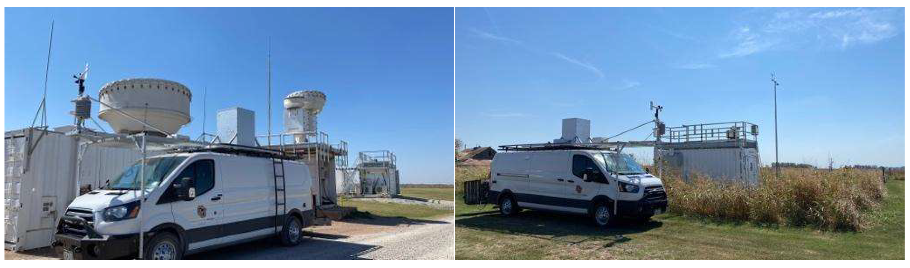
Figure 2.
Comparison of FFT between Lidar and Sonde; The blue, orange, and green lines in the figure depict the FFT of Doppler Lidar at altitudes of 0.285 km, 0.495 km, and 0.705 km, respectively, from 11:00 to 12:00. The red line represents the FFT spectrum of the radiosonde at 11:30, covering altitudes from 200 m to 1000 m.
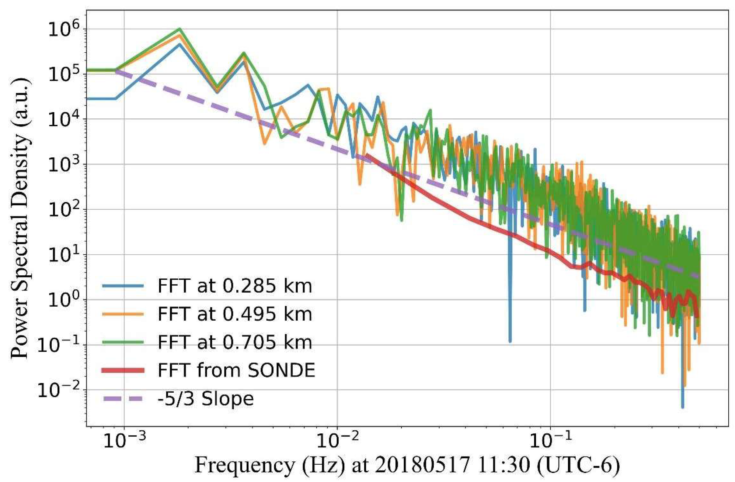
Figure 3.
FFT comparison at different times and altitudes on 20180517: (a) FFT around 9:00 AM at three different altitudes: 0.195 km, 0.586 km, and 1.425 km; (b) FFT around 2:00 PM at three different altitudes: 0.195 km, 0.586 km, and 1.425 km; (c) Vertical wind field data on 20180517 (red represents the three different altitudes around 09:00 in (a), black represents the three different altitudes around 14:00 in (b)).
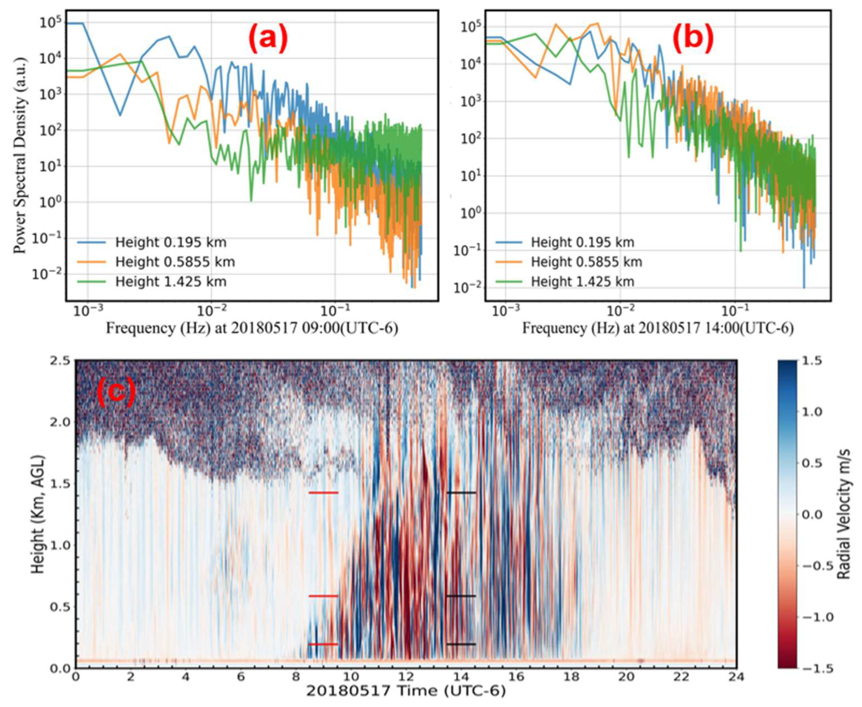
Figure 4.
The improved algorithm for estimating EDR.
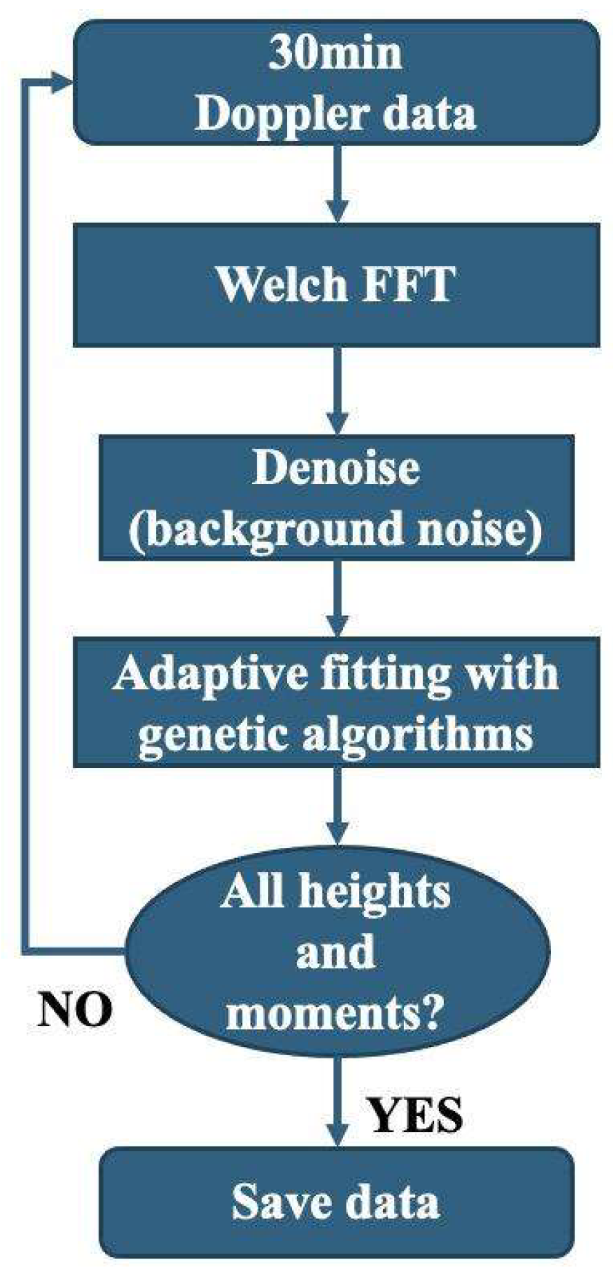
Figure 6.
Schematic of the diurnal evolution of the boundary layer based on EDR (from equation 4 in Section 2.1) and boundary layer height inversion on 20180517, with red dots indicating the boundary layer height (MLH). (a) Doppler lidar error, (b) vertical wind variance after wavelet analysis, (c) turbulent dissipation rate, (d) relative error, (e) vertical wind field from Doppler lidar.
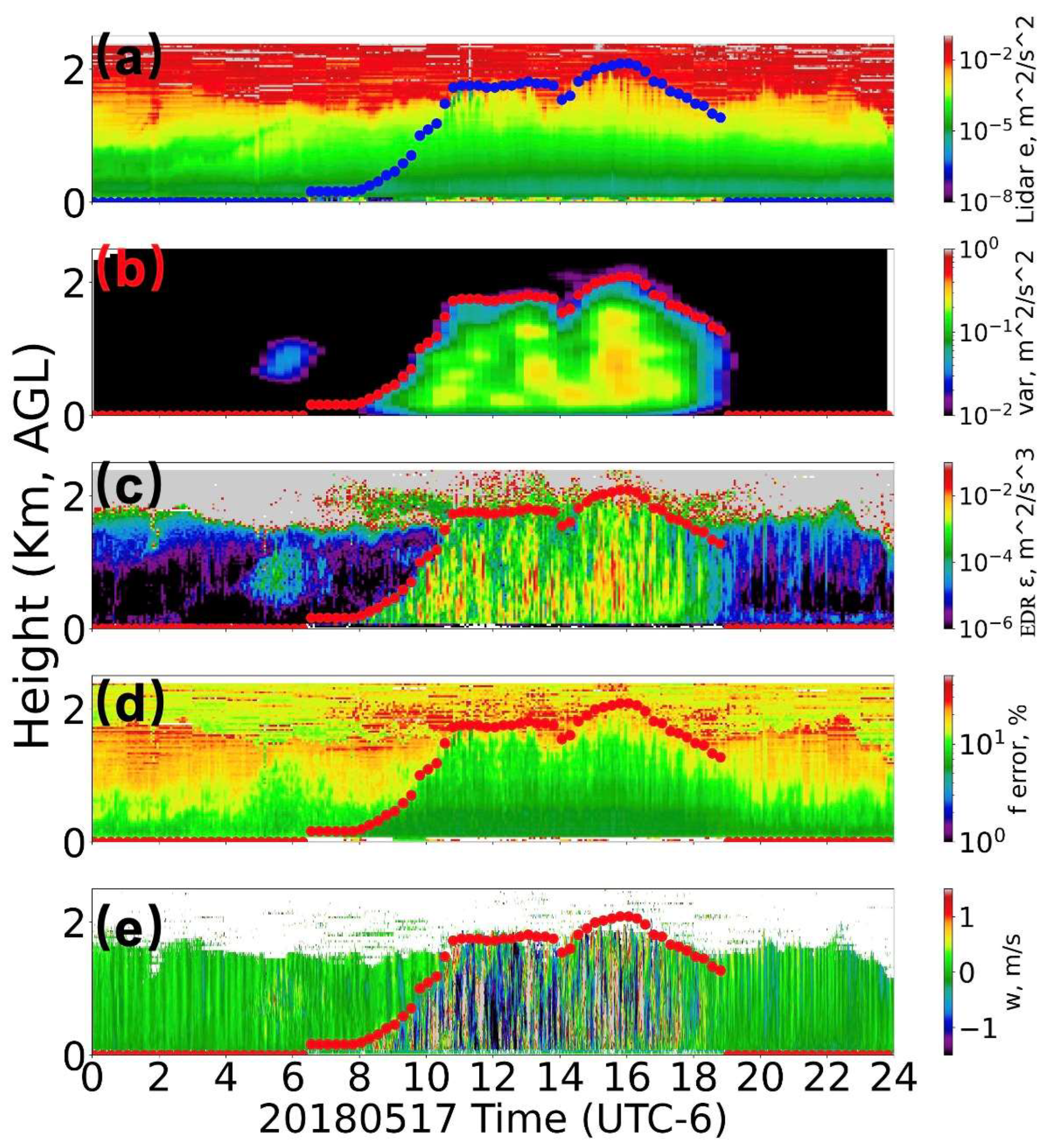
Figure 7.
EDR (from improved FFT method in Section 3.3) case analysis of LLJ (lower lever jet) from 20230416 to 20230419 at ARM SGP C1 site. The subplots from top to bottom are as follows: (a) Vertical wind field; (b) Vertical wind field variance; (c) EDR; (d) Horizontal wind speed; (e) Horizontal wind direction.
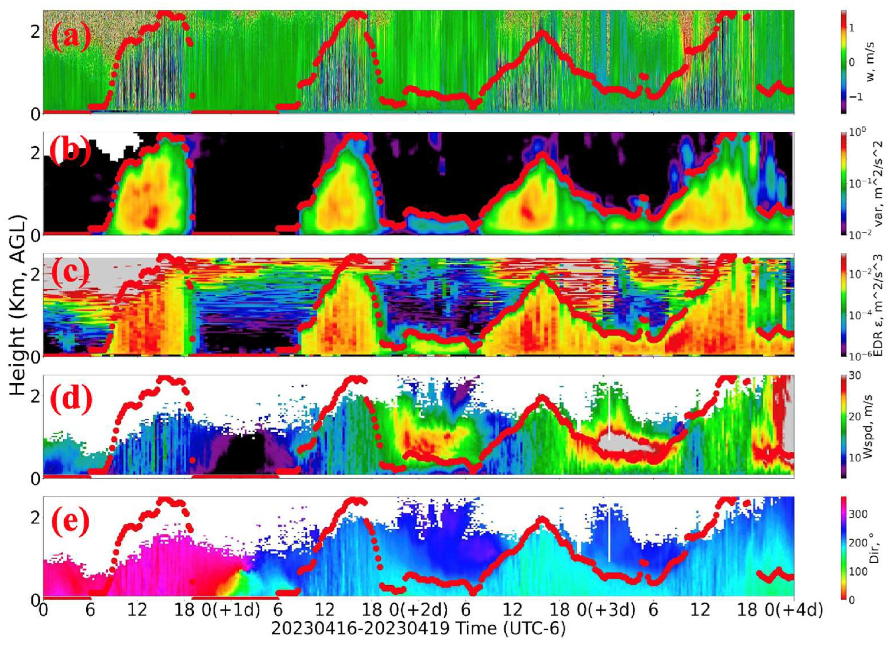
Figure 8.
Seasonal variation of median EDR with altitude at different ABL Development Stages: From sunrise to sunset at four representative height fractions (0.1Zi, 0.3Zi, 0.5Zi, and 0.7Zi), as shown in Figure 7a–d (Zi is MLH; MAM: March–May, JJA: June–August, SON: September–November, DJF: December–February).
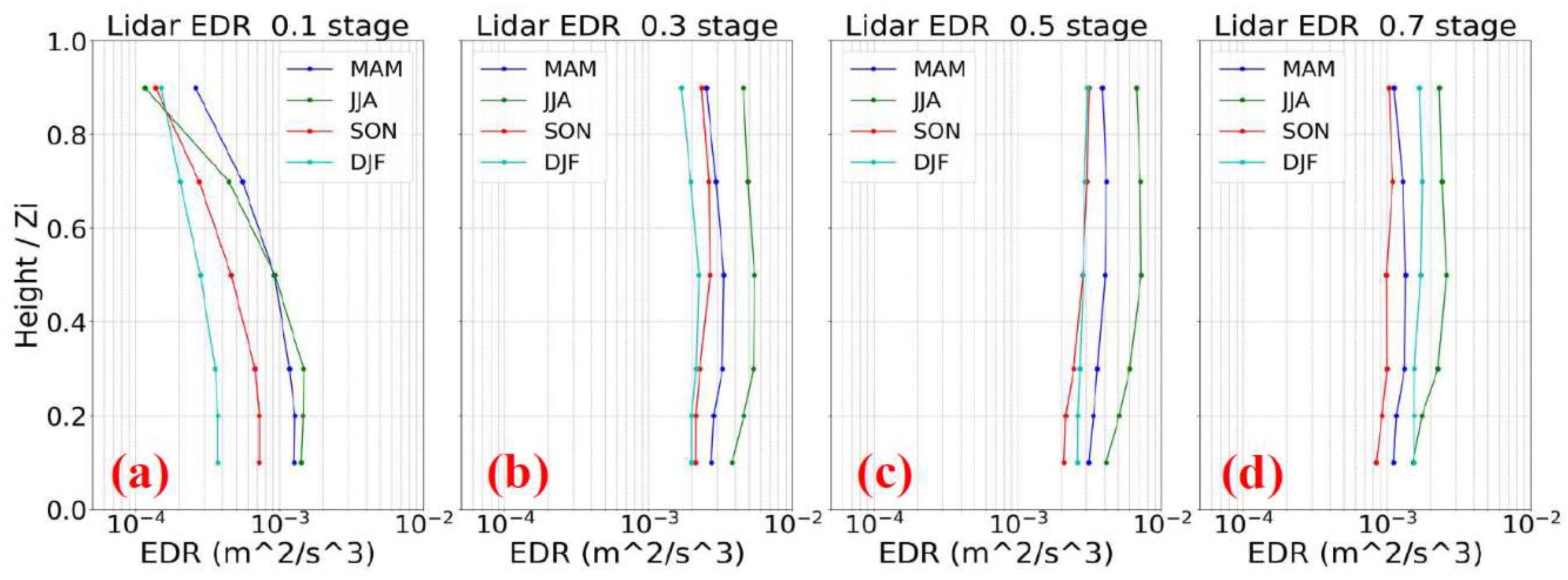
Figure 9.
Comparison of Vertical Velocity Between SGP Sites and ADL. ADL at C1 on 20230928: the three subfigures are vertical velocity from (a)SGP C1 Doppler lidar, (b) ADL (near C1 site) and (c) SGP E37 Doppler lidar. ADL at E37 on 20230930: the three subfigures are vertical velocity from (a)SGP C1 Doppler lidar, (b) ADL (near E37 site) and (c) SGP E37 Doppler lidar. The Red dots are MLH.
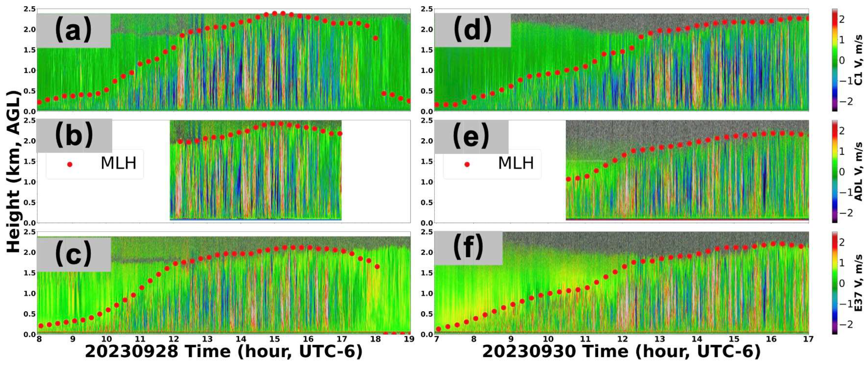
Figure 10.
Comparison of EDR (from equation 4) between SGP Sites. (a-c) ADL at C1 on 20230928: the three subfigures are EDR from (a)SGP C1 Doppler lidar, (b) ADL (near C1 site) and (c) SGP E37 Doppler lidar. (d-f) ADL at E37on 20230930: EDR from (d)SGP C1 Doppler lidar, (e) ADL (near E37 site) and (f) SGP E37 Doppler lidar. The Red dots are MLH,.
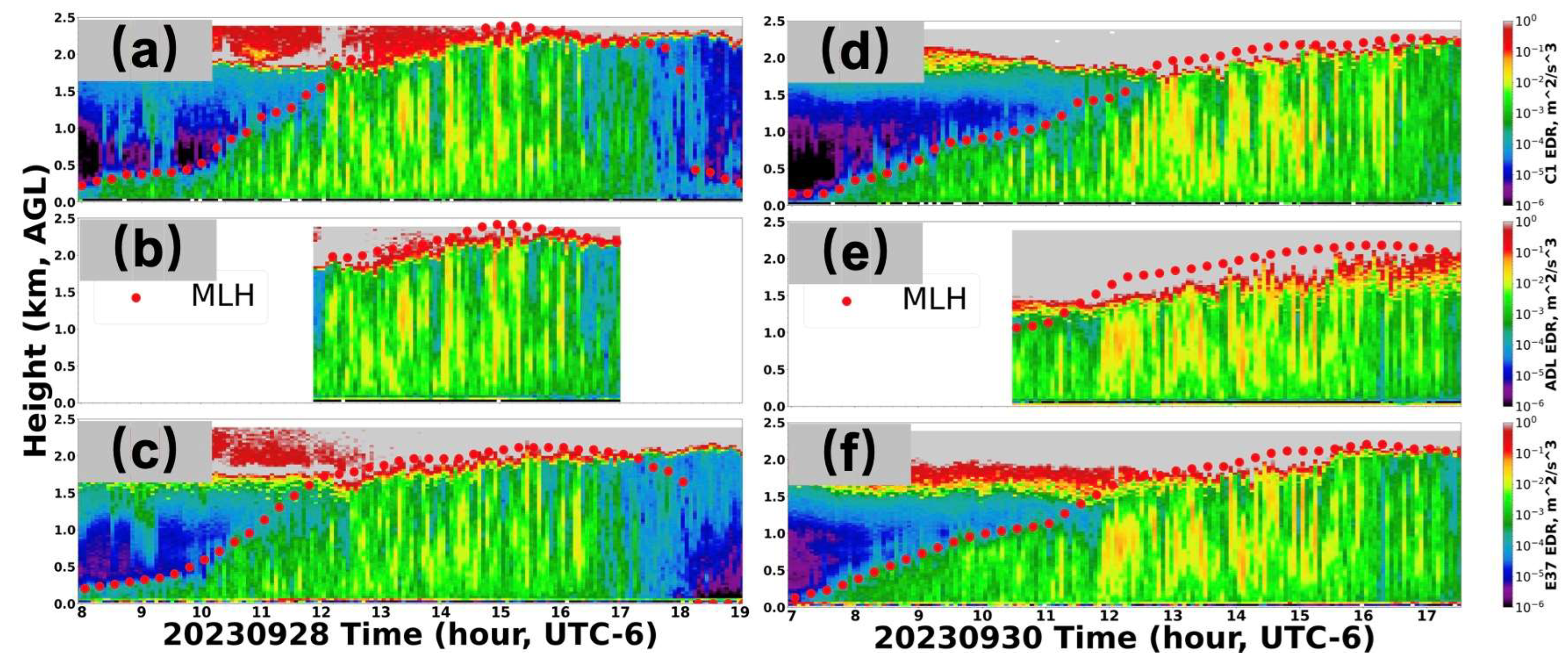

Table 1.
Doppler lidar and Sonde main parameters and datasets of ARM SGP C1 site.
| Parameters | SGP | PBLMAPS |
|---|---|---|
| Lidar Model | Stream Line Pro | ADL |
| Nyquist velocity (B) | ±19.4 m/s | ±80 m/s |
| Points per range gate (M) | 10 | 10 |
| Range gate resolution | 30 m | 18 to 90 m |
| frequency | 15 k | 10 k |
| Vertical wind | sgpdlfptC1.b1 sgpdlfptE37.b1 |
vertical wind, resolution 1-3s |
| Horizontal Wind | sgpdlprofwind4newsC1.c1 | / |
| Radiosonde | sgppblhtsonde1mcfarlC1.s1 | / |
Disclaimer/Publisher’s Note: The statements, opinions and data contained in all publications are solely those of the individual author(s) and contributor(s) and not of MDPI and/or the editor(s). MDPI and/or the editor(s) disclaim responsibility for any injury to people or property resulting from any ideas, methods, instructions or products referred to in the content. |
© 2025 by the authors. Licensee MDPI, Basel, Switzerland. This article is an open access article distributed under the terms and conditions of the Creative Commons Attribution (CC BY) license (http://creativecommons.org/licenses/by/4.0/).
Copyright: This open access article is published under a Creative Commons CC BY 4.0 license, which permit the free download, distribution, and reuse, provided that the author and preprint are cited in any reuse.


