
Submitted:
31 January 2025
Posted:
31 January 2025
You are already at the latest version
Abstract
This paper investigates the design optimization of high- and low-pressure axial-flow turbines within the context of a 50 MWe supercritical carbon dioxide (sCO2) Brayton power cycle, focusing on enhancing thermal efficiency and reducing costs for concentrated solar power applications. The study aims to evaluate and compare different loading design philosophies, emphasizing the balance between isentropic efficiency and mechanical stress. Through a analysis of design variables, the research identifies optimal turbine configurations that maximize efficiency while minimizing peak rotor stresses and overall volume. The results indicate that the selected non-dominant optimal solutions effectively exhibit a trade-off between efficiency and mechanical integrity. Notably, the optimal designs yield a 3% reduction in efficiency relative to the highest efficiency designs while achieving a 29% increase in peak rotor stress compared to the lowest stress designs. The findings reveal that for high-loading turbine designs, exceeding 90% efficiency as a design objective results in a significant increase in peak rotor stress, necessitating careful consideration of operational limits. Additionally, the paper presents Pareto fronts for non-dominating optimal solutions, highlighting the effectiveness of low-loading designs in maintaining a balance between efficiency and structural performance.
Keywords:
Supercritical CO2
; axial turbine
; mean line design
; design of experiments
; CFD modelling
1. Introduction
Supercritical carbon dioxide (sCO2) Brayton power cycles offer high thermal efficiency with a compact power cycle footprint (lower construction, transport, and maintenance costs) thanks to the favorable fluid properties of sCO2 compared to traditional technologies such as Rankine cycles which uses steam. For concentrated solar power (CSP) applications, the higher thermal efficiencies that sCO2 Brayton cycles offer could potentially lead to reduced solar field sizes and in turn lower plant construction and operating costs [1,2]. A primary factor that drives costs for sCO2 power cycles are the large recuperator heat exchangers [3], which are essential for achieving high thermal efficiencies. One approach to make sCO2 power cycles more economical is to reduce recuperator sizes by increasing turbine efficiencies [4]. Di Bella [4] has shown that a 2% increase in turbine efficiency for a 29 MWe power cycle can lead to a substantial 17% reduction in recuperator size. Therefore, it is essential that sCO2 Brayton cycle turbines are designed to maximize efficiency, whilst maintaining a small footprint to keep capital costs with regards to the turbine system low.
In the present work, a preliminary design analysis is performed for the high-pressure turbine (HPT) and low-pressure turbine (LPT) of an envisioned 50 MWe CSP sCO2 Brayton cycle. The objective is to investigate and comment on the thermal performance, mechanical stress and size differences between a high stage loading design philosophy, which offers a small and compact turbine package, and a low stage loading design philosophy which results in a highly efficient but potentially larger turbine package.
Numerous studies have examined the performance of sCO2 power cycle axial turbines. This discussion will briefly highlight selected key research findings. Salah et al. [5] performed a mean line design study for a 100 kW sCO2 axial turbine for CSP applications. The authors developed a mean line analysis tool which includes all the required loss models, similar to the present work, to design the small axial turbine and examine the impact of varying design parameters on turbine efficiency and size. The authors varied stage loading, flow coefficient and degree of reaction parameters, and found that an acceptable design could be achieved for a low flow coefficient of 0.2, a high stage loading coefficient of 1.4 and low degree of reaction of 0.0. Similar to the previous authors, Stepanek et al. [6] also performed a parametric preliminary mean line design analysis, but rather focused their efforts on large scale turbine units with shaft powers of 10-2000 MWe. The authors utilized the Nelder-Mead gradient-free optimization approach to design 460 high-performance axial turbines using a mean line approach with a reduced-order loss modelling technique presented by Dostal et al. [7] that only includes for trailing-edge and ventilation losses. The optimal turbine configurations revealed that most designs consist of 3 or 4 stages. Additionally, higher rotational speeds are beneficial for power levels up to 50 MWe, but beyond this threshold, they offer no significant advantage in terms of thermal efficiency compared to lower rotational speeds such as 3000 rpm. For these smaller higher-speed turbines, typical efficiency values were found to be approximately 87%. Recently Wang et al. [8] developed a detailed mean line model to evaluate sCO2 axial turbine performance for power levels ranging between 50-450 MWe. This study aimed to identify potential scaling laws for aerodynamic losses, such as profile and secondary losses, in relation to turbine shaft power. Using detailed loss model correlations from the literature, the authors derived scaling laws and demonstrated their validity through successful application. Furthermore, the authors found that as shaft power increases, irreversibilities reduce and that maximum turbine efficiencies could be found at pressure ratios of approximately 2. Abdeldayem et al. [1], investigated the flow path design of a 130 MWt sCO2 axial flow turbine that operated with SO2 dopant present within the working fluid. The mean line design utilized specific parameters optimized for thermal performance which included a flow coefficient of 0.5, a stage loading coefficient of 0.5, and a degree of reaction of 0.5. The designed turbine consisted of 14 stages and had a design point total-to-total isentropic efficiency of 92.9% and maximum rotor stress of less than 260 MPa. Building on the previous work, Salah et al. [9] investigated the off-design performance of the 130 MWt turbine using computational fluid dynamics (CFD) and mean line simulations. The authors found that the 14-stage axial turbine could operate at part-load conditions down to 88% of the design mass flow rate, corresponding to a drop in efficiency from approximately 93% at design conditions to 80% at the part-load conditions. Further turndown of the turbine mass flow rate was not possible in that the turbine started to produce negative shaft work. The primary cause of this was substantial flow separation in the latter stages of the turbine. The authors also compared the predictions of the part-load CFD simulations to the results produced using the mean line simulation tool, which utilizes the Aungier loss model set [10]. The results indicated that for flow coefficients below 90% of the design value the differences between the two models increased substantially.
In the present work a comprehensive mean line design analysis is presented, evaluating high- and low-loading design approaches for the HPT and LPT of a 50 MWe sCO₂ recompression Brayton power cycle featuring reheating and intercooling. The design analysis employs a design of experiments approach generating thousands of turbine designs by systematically sampling combinations of stage loading coefficients, flow coefficients, and mean blade speeds. Using the generated high- and low-loading design datasets for both the HPT and LPT, a surrogate model is fitted and used to identify turbine designs with the maximum efficiencies or minimum peak rotor stresses. Additionally, a multiobjective genetic algorithm is used to find the optimal designs for the high- and low-loading HPTs and LPTs based on maximizing efficiency and minimizing peak rotor stress. Once the preferred turbine designs for the high- and low-loading HPTs and LPTs have been identified, CFD simulations are performed to validate the mean line calculation results. The novelty of the present work lies in presenting a comprehensive design analysis and optimized parameters for both high- and low-loading design philosophies, applied to the HPT and LPT of a 50 MWe cycle each with specific turbine inlet conditions. The cycle is envisioned to operate with a single-shaft configuration at a rotational speed of 9000 rpm, posing unique design considerations. The mean line design, surrogate modelling and optimization codes were all developed in-house using the Julia programming language with CoolProp.jl [11], Roots.jl [12], Surrogates.jl and Metaheuristics.jl freely available libraries.
2. Materials and methods
2.1. Case study power cycle
In this study, design calculations are conducted for the high- and low-pressure axial turbines of a conceptual 50 MWe sCO2 recompression Brayton cycle, incorporating intercooling and reheating. The cycle layout is seen in Figure 1. The authors completed preliminary design calculations for the cycle and compressors, which are detailed in previous studies [13,14]. Following the mechanical design recommendations by Sienicki et al. [15], a single-shaft configuration has been selected for the current 50 MWe power cycle. Furthermore, the rotational speed of the shaft is fixed at 9000 rpm (rotational speed based on previous cycle and compressor designs research works).
The cycle is intended to operate with heat input from a CSP tower with molten nitrate salt used as heat transfer fluid. Nitrate salts have an upper operational temperature limit of approximately 590°C. To ensure safe operation, the turbine inlet temperature is set at 550°C, providing a safety margin below the specified temperature limit [16]. The inlet conditions for the two turbines and the required pressure ratios per machine are reported in Table 1. These conditions along with specified design parameters such as stage flow coefficient and stage reaction are used as the inputs to the developed computer model used to perform the preliminary design analysis of the turbines.
2.2. Mean line design calculations for sCO2 axial-flow turbines
The mean line computer model is utilized to perform thermodynamic, kinematic (velocity diagrams) and sizing calculations using various aerodynamic loss models (e.g., profile losses) and geometrical correlations (e.g., blade solidity) along the midspan of the axial turbines. The objective of the model is to generate a preliminary design of an axial turbine based on the inlet thermodynamic conditions (Table 1) and specified design parameters. These design parameters are the user-specified stage loading coefficient , flow coefficient , stage reaction and mean radius blade speed [m/s]. The equations for these design parameters are shown below [17].
In Equation (1), [J/kg] is the specific stage work extracted, which is equal to the change in stagnation enthalpy across the stage, [m/s] is the axial velocity within the turbine stage and [J/kg] is the static enthalpy change across the stage rotor. In the present work repeating turbines are designed, therefore, the flow coefficient is taken as constant throughout the turbine and set equal to the user input value. The user-specified stage loading coefficient, now indicated as , is used to estimate the number of stages required to achieve the desired pressure ratio as seen in Equation (2), where [J/kg] is the specific work extracted by the complete turbine set [18]. can be calculated using the inlet thermodynamic conditions, pressure ratio and total-to-total isentropic turbine efficiency, . The total-to-total isentropic efficiency, in turn, is estimated from the thermodynamics and aerodynamic losses of each stage, which will be discussed later.
Once the number of stages is estimated for a turbine, the user-specified reaction (indicated with an asterisk as ) and loading coefficients are directly used for the first stage. The remaining work is then equally divided per stage, as shown in Equation (3). The reaction coefficients for the stages following the first one are calculated implicitly, as will be shown in Section 2.2.1. This results in the reaction and loading coefficients for stages following the first stage to be different compared to the user-specified design parameters and .
2.2.1. Stage flow kinematics
With the flow and loading coefficients for each stage known, all the necessary absolute and relative flow angles, as well as the stage reactions, are calculated. Figure 2 defines the flow angles applied in the current work along with selected geometric parameters, which will be discussed in Section 2.2.3.
For the first stage, the inlet absolute flow angle is set [rad] and, as mentioned, the stage reaction set to the user-specified value, where the subscript indicates that it is for the first stage. For subsequent stages, the stage inlet absolute flow angle is simply set to the previous stage outlet absolute flow angle, , where the subscript indicates the stage index and the subscripts indicate the station within the stage. The degree of reaction per stage (excluding the first stage) is then calculated as shown in Equation (4), where it should be noted that the flow coefficient is a user-specified value and is taken as constant throughout the turbine [18].
Using the stage loading and reaction rules mentioned above, the stator outlet (station 2) and rotor outlet (station 3) absolute and relative flow angles of the stage can be estimated using Equation (5) [19]. In Equation (5), and [rad] are the rotor inlet and exit relative flow angles and [rad] is the rotor inlet absolute flow angle.
The velocities at each station within a stage are calculated as shown in Equation (6), where , and [m/s] are the stator inlet, rotor inlet and rotor exit (subscripts 1, 2 and 3 respectively) absolute tangential velocities (tangential component indicated by subscript ). , and [m/s] are the absolute velocities for the indicated stations. and [m/s] are stations 2 and 3 relative tangential velocities and relative velocities respectively.
2.2.2. Stage thermodynamics
By applying the calculated loading coefficients and the velocities at each station, the stagnation pressures and enthalpies within each stage can be determined. Assuming steady-state behavior, the mass flow rate is assumed to be constant throughout the turbine, therefore, the energy balances for the stator and rotor within a stage can respectively be written as
and [J/kg] are the stagnation enthalpies at stations 1, 2 and 3 respectively and is the change in stagnation enthalpy across the rotor of the specific stage. For the stage this change in stagnation enthalpy is calculated as . To find the stagnation pressure at the exit of the stator [Pa], first the stator exit static pressure [Pa] is implicitly solved using Equation (8) along with a fluid property database to evaluate where is the stator inlet entropy, in turn, evaluated as . In Equation (8), [J/kg] is the static enthalpy at the stator exit which is calculated as and is the specific stage stator efficiency. The stator efficiency is calculated using the aerodynamic losses per stage which will be discussed in Section 2.2.4.
Using the stator exit static enthalpy and pressure the corresponding entropy can be evaluated as and thereafter the stator exit stagnation pressure using . The rotor exit pressure is calculated by implicitly solving Equation (9).
In Equation (9), the rotor exit isentropic stagnation enthalpy is evaluated using a fluid property database as [J/kg], where is determined from the in Table 1. In the previous equation, is the stage efficiency that, similar to the stator efficiency, is estimated using the aerodynamic losses which will be discussed later.
After the stagnation pressures and enthalpies per station in each stage of the turbine are estimated the total-to-total turbine isentropic efficiency is calculated using Equation (10). The remaining fluid properties, indicated by for properties such as densities and temperatures, can be evaluated simply by using the calculated station entropy and static enthalpy and a fluid property database as
With the thermodynamic properties, velocities and flow angles at each station known the geometrical dimensions of the turbine stages can be sized. This will be discussed in the next section.
2.2.3. Geometric sizing and stress calculations
In Figure 2, selected geometrical dimensions of the turbine blade cascade are indicated. [m] is the blade chord length (separate values for rotors and stators indicated as and respectively), [m] is the axial blade chord length, [m] is the maximum blade thickness value, [m] is the blade row pitch, is the blade row solidity and is the blade row stagger angle. The sizing of these variables and others will now be discussed.
For the current turbine designs, flaring of the hub and casing radii are applied to ensure a constant mean diameter [m] which consequently results in a constant mean blade speed throughout the turbine. The mean diameter is calculated using Equation (11).
The blade heights at the stations 1, 2 and 3 of a stage is estimated using Equation (12), where and [m2] are the passage flow areas and and [kg/m3] are the densities at the indicated stations within a stage.
The average stator and rotor blade heights are then taken as the linear average between the inlet and outlet blade row heights. The average stator blade height of a stage is calculated as and for the stage rotor as . Next the rotor and stator boss ratios are calculated using the relations shown in Equation (13) [18].
To estimate the axial blade row aspect ratios, , the curves of Sammak et al. [20] are used. In the equation below, is an adjustment factor introduced in the present work. After investigation, it was found that the blade dimensions calculated using the curves of Sammak et al. lead to excessive gas bending stresses across large portions of the analyzed design parameter ranges. Therefore to reduce the gas bending stress, the blade chords are extended by reducing the axial blade row aspect ratios. This is achieved by including the adjustment factor . For a factor of , more reasonable gas bending stresses were observed while the calculated average axial blade row aspect ratios fell within the recommended range of 1.0-2.0 [17]. This will be discussed further in the results section.
The axial blade chords and can be calculated by simply dividing the average stator and rotor blade heights () by their respective axial blade aspect ratios (). To determine the blade chords, first the stator and rotor stagger angles, [rad], are estimated using the correlation of Tournier and El-Genk [21] shown in Equation (15), where [deg] is the blade inlet angle. For the stator blade rows is simply taken as the inlet absolute flow angle and for the rotor blade rows the corresponding inlet relative flow angle .
The expressions for the coefficients in the above correlation are provided in Equation (16).
where [deg] is the blade exit angle. For the stators, this is taken as , while for the rotors, the effect of flow deviation is considered. Therefore, the rotor blade exit angle is calculated as where [deg] is the deviation angle at the rotor exit. Once the stagger angles for the blade rows of a stage are found the stator and rotor blade chords are calculated as and respectively. To calculate the rotor exit deviation angle, per stage, the correlation of Wang et al. [22] was utilized, shown in Equation (17).
In Equation (17), [m] is the rotor blade maximum thickness and is the rotor exit Reynolds number calculated as where [] is the molecular dynamic viscosity of the fluid evaluated at station 3 of a specific stage.
The solidities for the blade rows are calculated using the optimal blade solidity correlations provided by Aungier [10]. The optimal solidity for axial-flow entry stators and impulse blading is calculated using the respective expressions in Equation (18), where [deg] is the exit relative flow angles. For a stator row and for a rotor .
The effective solidity for an actual blade row is calculated using Equation (19), where [deg] is the blade row inlet blade angle. For the stator and for the rotor .
Stator and rotor blade row pitches are calculated as and respectively. The number of blades per row is then calculated as .
For the turbines designed in the current work, the trailing edge thicknesses is chosen to be 2% of the blade row pitch [18] and the tip clearance for both the stator and rotors is 1.5% of the average blade row height. The maximum blade thickness is estimated using trends provided by Krumme [23]. These trends are digitized and the correlations can be found in Equation (20), where is the chord length for either the rotor or stator and [deg] is the gas deflection angle within the blade row.
With the turbine dimensions sized the centrifugal and gas bending stresses of the rotor rows are estimated using equations (21) and (22) respectively [19].
In Equation (21), [kg/m3] is the blade material density and . In Equation (22), is the amount of rotor blades in a stage and is based on empirical curves proposed by Ainley. These empirical curves have been digitized and fitted. The expression for and accompanying correlations are found in Equation (23), where [deg] is the rotor blade row camber angle.
In the present work the turbine blade material is taken as Ni-Cr-Co (Inconel 718) which has a density of 8000 kg/m3 [5].
2.2.4. Aerodynamic losses
The aerodynamic models used in the current work which accounts for profile, secondary, trailing edge and tip clearances losses are based on the work of Kacker and Okapuu [24], Benner et al. [25,26] and Yaras and Sjolander [27]. For the sake of brevity, only key components of the model equations will be presented here.
The total blade row loss coefficient is calculated using Equation (24), where is the total pressure loss coefficient, the combined profile and secondary loss coefficient, the trailing edge loss coefficient and the tip clearance loss coefficient.
The combined profile and secondary loss coefficient is determined using the formulation established by Benner et al. In the Equation below, [m] is the spanwise penetration loss factor, is the profile loss coefficient and is the secondary loss coefficient.
The profile loss coefficient is calculated using the correlation of Zhu and Sjolander [28] shown in Equation (26) and is specifically only for design point evaluations (zero incidence). In Equation (26), is the inlet modification factor which is set to 0.667 for all blade rows except the first stator row where it is set to 0.825. In the present work the calculation of the Mach number correction factor and shock loss pressure coefficient are similar to what is shown in Tournier and El-Genk [21].
The Reynolds number correction factor is calculated using the approach proposed by Aungier [10], which accounts for surface roughness effects. In Equation (27), is the blade row exit Reynolds number which for the stator is and for the rotor [relation shown below Equation (17)]. is the critical Reynolds number and is calculated as where [m] is the surface roughness. For the present work the blade surface roughness was set to 50 μm [18].
The Ainley and Mathieson loss coefficient and modification thereof was calculated using the approach of Zhu and Sjolander [29] as seen in Equation (28). In this equation, similar blade () and flow () angle assignments as Equation (19) are used. is a modification factor proposed by the authors of the model and is set to 1 if and equal to -1 if . The correlations for and can be found in [18].
The secondary loss coefficient is calculated using Equation (29), where [rad] and [rad] are the inlet and exit flow angles for the blade row, which for stators are the absolute flow angles and for the rotors the relative flow angles. The calculation of the aspect ratio factor and the inlet end wall displacement thickness [m] is performed using the relations found in [21,25], respectively.
The spanwise penetration depth factor is calculated using the correlation of Benner et al. [26] shown in Equation (30). The Equation for the tangential loading parameter can be seen in the original work of the authors of the correlation.
The clearance losses are calculated using the correlations provided by Yaras and Sjolander [27]. The clearance loss is calculated using with being the tip loss coefficient and the gap loss coefficient. Equation (31) below shows the correlation used for the tip loss coefficient in the present work.
In the previous equation, was set to 0.5, as recommended by the authors of the correlation for mid-loaded blades and the tip gap discharge coefficient was selected as . The mean velocity vector angle is calculated as . To calculate the tip loss coefficient the theoretical blade lift coefficient is estimated using Equation (32) [30].
The gap loss coefficient is calculated using Equation (33), where and for mid-loaded blades.
The final loss coefficient to consider is the trailing-edge losses. In the present work the correlations established by Kacker and Okapuu [24] will be utilized. This loss correlation is for the corresponding enthalpy loss coefficient rather than pressure loss coefficient, as shown in Equation (34).
The correlations for the enthalpy loss coefficients for the axial entry stators and impulse blading can be found in [21]. To convert the enthalpy loss coefficient to a pressure loss coefficient, Moustapha et al. [31] recommends an expression, which theoretically is only applicable for ideal gases. Although the error accompanying this assumption is relatively small, a real gas approach to convert the losses is provided here. Using the state isentropic density [32] it can be easily shown that the enthalpy loss and pressure loss coefficient are related as shown in Equation (35) for a stator and rotor respectively.
In the previous equation, [Pa] and [Pa] are the rotor exit and inlet relative stagnation pressures, [J/kg] the rotor exit relative stagnation enthalpy and [kg/m3] the rotor exit relative isentropic density.
2.2.5. Solution strategy
To generate a converged solution for the above thermodynamic, kinematic, geometric and aerodynamic loss equations, a successive approximation solution strategy is implemented. This approach begins by guessing an initial value for , which, along with the inlet thermodynamic boundary conditions, is used to estimate the specific shaft work of the turbine, . Additionally, the values for and for each stage are initialized to guessed values. The solution procedure is shown in Figure 3.
For the stator the total loss coefficient is used to update the blade row exit pressure, and in turn stator efficiency, using the calculation process shown in Equation (36).
Similarly the stage efficiency is calculated using the rotor total pressure loss coefficient and the calculation steps shown in Equation (37), where [J/kg] is the rotor inlet relative stagnation enthalpy.
2.3. Turbine parameter sampling and surrogate modelling
The typical ranges and values for sCO2 axial turbine design parameters found in literature can be seen in Table 2. These ranges and values are used to inform the various analyses performed in the current work.
To analyze the effect of the design parameters on the thermal performance, peak rotor blade stresses and geometric dimensions of the HP and LP turbines, a design of experiments is conducted. This involves generating 5000 sample sets, each with varying values for stage reaction, flow coefficient, and mean blade speed for both turbines. A mean line design analysis is then carried out for each sample under both high and low loading conditions. For the high loading cases, the specified stage loading was set at 1.0, while for the low loading cases it was set at 0.4. The analysis considered a stage reaction range of 0.0 to 0.6, a flow coefficient range of 0.2 to 1.0, and a mean blade speed between 170 and 250 m/s. The selected mean blade speed range is increased in the analysis to allow a somewhat larger design space within which optimal values can be obtained.
Turbines with low stage loadings will generally achieve higher efficiencies compared to higher loaded machines and given that the cycle under investigation is intended for land-based power generation, the decision is made to limit the higher loaded machines to a stage loading of 1.0. This ensures a balanced trade-off between turbine size and thermal performance for the comparative analysis between the higher and lower loaded turbine designs.
To generate the data points for the analysis, the Sobol sampling algorithm [33] was utilized to ensure good coverage across the 3-D space of stage reaction, flow coefficient and mean blade speed. After creating the sample sets and generating discrete results through mean line design analysis runs, both the results and input sets were fed into a Kriging surrogate modeling framework. This approach was used to develop continuous functions for interpolation purposes to perform multiobjective optimization and iso-surface visualizations [34]. The Kriging model takes the sample sets as inputs and outputs key performance metrics namely efficiency, peak rotor blade stress, and total machine volume.
To identify non-dominating optimal solutions the developed surrogate models are utilized along with the NSGA-II multiobjective genetic algorithm [35] that sets out to maximize the isentropic efficiency and minimize peak rotor stresses by changing design flow coefficients, degree of reactions and mean blade speeds. The preferred optimal solutions are selected based on the minimal Euclidean distance between the non-dominating optimal points and the ideal points for each machine and loading level [36]. In addition to the optimal points the surrogate models are used to identify the machine designs that have the maximum efficiency and minimum rotor stresses. These results will be shown in the results and discussion sections for the LPT and HPT respectively.
It is important to note, for the high loading designs, samples can exist where . If this is the case the stage loading is adjusted such that , therefore, the machines will only have a single stage.
2.4. Computational fluid dynamics modelling of sCO2 axial-flow turbines
The turbine parameter sampling and surrogate modeling efforts described above results in the identification of optimal designs for high- and low-loading LP and HP turbines. To validate the reliability of the mean line analysis results for these selected designs, CFD simulations are performed. The simulations are performed using ANSYS CFX 2024 R2 software, following a systematic pipeline that includes geometry creation, grid generation, and the configuration of physics and solver settings.
The geometries of the turbine blades are generated using the method described by Aungier [10]. This approach utilizes general outputs from the mean line design analysis code such as inlet and exit blade angles, stagger angle, throat width, and the number of blades per blade row. These parameters are used to define the pressure and suction side profiles through third-order polynomial curves and specified coordinates for each blade row. The blade camber angle and thickness distribution are then extracted from these generated polynomial curves and used along with ANSYS BladeGen to generate the 3D blade profiles for each turbine blade row. It should be noted that for sake of simplicity the current work only considers straight blades across the blade row spans, similar to the work of Shi et al. [37].
To minimize the computational mesh size, simulations were conducted using a single blade passage per blade row. The blade row geometries created in BladeGen for the high- and low-loading HP and LP turbines were imported into ANSYS TurboGrid for grid generation. Once the blade row meshes for a single turbine (e.g., high-loading HPT) are generated, they are imported into ANSYS CFX. 3D steady-state simulations under full load conditions (Table 1) were performed using the SST turbulence model with the automatic wall treatment [1,37]. The advection quantities were discretized using higher-order schemes, whereas the turbulence fields were discretized using a first-order scheme. Interpolation between successive blade row meshes were performed using the frozen rotor model. To capture the variations in CO2 fluid properties within the computational domain, a real gas property table is generated using the Refprop software and imported into CFX. The simulations employ a combination of total temperature and pressure as inlet boundary conditions and mass flow as outlet boundary condition. To ensure not only convergence of solved balance Equation residuals but also monitored variables such as isentropic efficiency and exit absolute pressure the convergence criteria of all simulations is set to a value of 1e-6.
3. Results and discussions
3.1. High-pressure turbine mean line design results
Figure 4 presents iso-surface contour plots of isentropic efficiency as a function of stage reaction, flow coefficient, and mean blade speed. These plots are based on the outputs of the Kriging surrogate model constructed using the design of experiments dataset for the high- and low-loading HP turbines. Comparing the ranges of the calculated efficiencies, it is seen that the low loading turbines have higher achievable efficiency values compared to the high loading machines, specifically in the stage reaction range of 0.4-0.6, flow coefficient range of 0.2-0.5 and blade speed range of 170-240 m/s. These ranges will be referred to as the high efficiency ranges from here on. Within these ranges, the average rotor total pressure loss coefficient for the high-loading cases is . For the highly loaded designs within the mentioned range, the highest average loss contribution is the tip clearance loss, , followed by the secondary loss coefficient, . For the low-loading cases within the high efficiency ranges the average total rotor pressure loss coefficient is . For the low-loading turbines the highest average loss contribution is the secondary loss, , closely followed by the tip clearance loss, .
The average tip clearance loss for the high-loading cases within the mentioned high-efficiency ranges is 77% higher than in low-loading designs, primarily due to the higher gas deflection angles within the high loading designs. The average gas deflection angle within the low loading rotors is 22 degrees compared to 49.5 degrees for the highly loaded machines. This leads to the theoretical blade lift coefficient [Equation (32)] being significantly larger for highly loaded machines, and in turn the tip loss coefficients. For the secondary losses between the two loading set points, the calculated quantities for the high- and low-loaded designs are relatively similar with a 12% relative difference.
Figure 5 (top) shows the iso-surface contour plots for the peak stage combined rotor stresses [] within the various designed turbines for both the high- and low-loaded conditions. Figure 5 (bot) shows the total-to-total isentropic efficiency of the designs as a function peak rotor stress, chord length and mean rotor blade height (marker size).
From Figure 5 (top) it is interesting to note that the peak stresses for the highly loaded design cases occurs at high flow coefficients and low stage reactions, whereas for the low-loading machines the peak stresses are found at low stage reactions and moderate flow coefficients between 0.3-0.6. This is since at lower stage loadings the gas deflection angles are smaller compared to the highly loaded designs. This in turn results in lower stagger angles and smaller chord lengths, which [as seen in Equation (22)] results in higher gas bending stresses. For both stage loading design setpoints, the minimum stresses are observed within flow coefficient ranges of 0.2–0.5, stage reaction ranges of 0.4–0.6, and high mean blade speeds above 180 m/s. These design parameters align closely with the high efficiency ranges. Within these high efficiency ranges, the high-loading designs exhibit peak rotor stresses ranging from 125 MPa to 810 MPa, while the low-loading designs show peak rotor stresses between 150 MPa and 850 MPa. The higher peak rotor stress range in low-loading cases are generally attributed to increased gas bending stresses for certain design parameter combinations that result in smaller chords and lower stagger angles. However, within the subsets of design parameters that yield the highest efficiencies the low-loading designs exhibit lower peak rotor stresses compared to the highest efficiency high loading designs. The reduced stresses at high mean blade speeds for both stage loading designs are attributed to the increased meridional velocity for a given flow coefficient through the turbine [as seen in Equation (1)]. This results in shorter blades and smaller flow areas, thereby decreasing centrifugal and gas bending stress. Thus to lower blade stresses, higher mean blades speed are required, but at very high blade speeds turbine efficiencies can suffer.
Figure 5 (bot), shows that for both the high and low loaded designs, as the average rotor chord length (x-axis) reduces the peak combined rotor stresses increases. For high-loaded designs, peak efficiency values are achieved with chord lengths between 55 mm and 65 mm, while for low-loaded designs, peak efficiency values are observed across a broader range of chord lengths, from 40 mm to 65 mm. Within these peak efficiency zones (circled in black), low-loading designs demonstrate the ability to achieve not only higher efficiencies but also lower peak stresses. This can be ascribed to the smaller change in absolute tangential velocities, , across the rotors in combination with relatively large chord lengths which are achieved for high rotor boss ratios and tall rotor blades.
As seen in Figure 6 for the design parameter inputs outside the high efficiency ranges, the gas bending stresses dominate. This is mainly since at these design specifications the chord lengths of the rotor blade rows become small, resulting in high gas bending stresses. It should be noted that even inside the high efficiency ranges the gas bending stresses also play a significant role as observed by [5]. An additional factor that contributes to these high gas bending stresses is the high mass flow rate combined with significant change in absolute tangential velocity through the rotor that results in large stresses.
The generated mean line analysis data enabled the identification of design parameter combinations for both high- and low-loading cases that satisfy specific user-defined requirements. Specifically, the parameters were determined for the individual design achieving the lowest peak rotor stress and separately for the individual design achieving the highest isentropic efficiency. These design points are shown in Table 3.
For the two highest efficiency designs, it is seen that the low loading turbine design achieves not only a 3.8% higher efficiency compared to the high loading design, but also a 43% lower combined peak rotor stresses. In both high and low-loading designs, high stage reaction and low flow coefficients are preferred. Additionally, lower mean blade speeds are desirable, as they lead to larger blade heights, which reduce secondary loss effects and improve isentropic efficiency. Due to the lower stage loading in the low-loading design, the number of stages is significantly greater compared to the high-loading design. This results in nearly a 50% increase in turbine volume of the low-loading design compared to the high-loading design. The turbine volumes are estimated as truncated cones, based on the casing diameters of the first and last stages.
For the two designs with the lowest stress values, both scenarios favor high mean blade speeds to reduce centrifugal stresses by shortening rotor blade heights and thus flow areas. The high-loading design achieves a lower peak rotor stress compared to the low-loading design. This is due to reduced gas bending stresses in high-loading configurations at higher mean blade speeds, where taller rotor blades result in larger chords. In contrast to the highest-efficiency designs, the lowest-stress designs exhibit significant differences in flow coefficients and stage reactions between the high- and low-loading configurations, emphasizing the distinct factors influencing peak rotor stresses. Lastly, both low stress designs suffer approximately 5.5% reduction in efficiency compared to the highest efficiency designs.
Due to the differences in isentropic efficiencies and peak rotor stresses among the previously discussed design options, optimal designs were identified for both high- and low-loading turbine configurations. These optimized designs are listed in the last two rows of Table 3. The optimized designs for both high- and low-loading configurations favor stage reactions and flow coefficients of approximately 0.59 and 0.2, respectively. The primary input variable that differs significantly between the two loading designs is the mean blade speed. This difference arises because the low-loading design inherently tends to experience higher gas bending stresses. To combat this, the optimization algorithm increases the mean blade speed which increases the boss ratio and in turn the chord lengths, which drives down the bending stresses. Although the low-loading optimal design is a larger turbine compared to its high-loading counterpart, it achieves higher isentropic efficiency and lower peak rotor stresses, making it the more desirable option under the design operating conditions. When comparing the optimal designs to other design scenarios, it is observed that, on average, the optimal designs result in a 3% reduction in efficiency compared to the highest efficiency designs. In contrast, when compared to the lowest stress designs, the optimal designs show a 29% increase in peak rotor stress. This represents a well-balanced trade-off between stress reduction and efficiency maximization.
To gain further insights into the optimization of the two loading design options, the Pareto fronts of non-dominating optimal solutions are plotted and shown in Figure 7. The results indicate that for the high-loading design, any efficiency increase beyond approximately 90% incurs a significant penalty in peak rotor stresses. Specifically, the gradient of the Pareto front above 90% is 86 MPa per percentage point of efficiency, meaning a 1% increase in efficiency results in an 86 MPa rise in peak rotor stress. In contrast, the low-loading design exhibits a less steep gradient of 31.9 MPa per percentage point of efficiency at higher efficiency levels, again highlighting the favorability of the low-loading design.
Generally, it can be seen assessing all the design scenarios in Table 3 that the high-loading designs result in significantly more compact turbines, but at the cost of lower efficiency. High-loading designs achieve a 10–55% reduction in turbine volume, depending on the design scenario (highest efficiency vs. lowest rotor stress), with a corresponding decrease in isentropic efficiency of 2.9–4%. However, from the perspective of peak rotor stresses, high-loading designs offer no distinct advantage over low-loading designs. Typically the peak stress for Ni-Cr-Co alloy is taken as 303 MPa [5] and often it is desirable to keep the peak stress below 260 MPa [1]. Therefore, the peak rotor stresses of the two highest efficiency designs are outside the allowable stress limit.
3.2. Low-pressure turbine mean line design results
Figure 8 shows the iso-surface contour plots of isentropic efficiency as a function of stage reaction, flow coefficient, and mean blade speed for the LP turbine designs. Similar trends are seen for the LP turbines as for the HP turbine trends in Figure 4, where the highest efficiencies are found for flow coefficients between 0.2-0.5, stage reaction between 0.4-0.6 and mean blade speeds above 170 m/s. The LP turbine designs achieve higher efficiencies compared to the HP turbine designs within the specified ranges. The average isentropic efficiency is 89.6% for high-loading HP turbines, compared to 90.6% for high-loading LP turbines within the high efficiency ranges. Similarly, for low-loading designs, HP turbines achieve an average efficiency of 91.2%, while LP turbines reach 93.1% within the high efficiency ranges. As previously mentioned, within both LP and HP turbine design datasets, the low-loading configurations achieve the highest isentropic efficiencies.
Within the above-mentioned high efficiency ranges the average total rotor pressure loss coefficients for the high- and low-loading LP designs are and respectively. For the high-loading designs within the above-mentioned ranges, the highest aerodynamic loss is the tip clearance loss with an average value of followed by the secondary loss with an average value of . For the low loading designs the main losses are and .
Similar to the HPT designs, the primary difference in tip loss coefficients between the high- and low-loading designs arises from variations in mean gas deflection angles, which significantly impact the blade lift coefficients. The mean high-loading rotor gas deflection angle within the mentioned ranges is 49 degrees and for the low-loading designs it is 21.8 degrees. As with the HPT designs, the secondary loss coefficients remain similar across the different loading configurations. An interesting observation is that the calculated profile loss coefficients, , are notably small (between 0.0-0.005) for the high- and low-loading HP turbine designs, as well as the low-loading LP turbine designs. However, for the high-loading LP turbine designs, within the specified high efficiency ranges, the mean profile loss coefficient is comparatively higher, . This observation is most likely due to the higher gas velocities within the highly loaded LP turbine due to the lower gas densities.
Figure 9 (top) shows the iso-surface contour plots of combined peak rotor stress for the high- and low-loading LP turbine designs and Figure 9 (bot) isentropic efficiencies as a function of mean rotor chord length (x-axis), peak rotor stress (y-axis) and mean rotor blade height (marker size).
The combined peak rotor stresses plots for the LP turbines have very similar trends to that of the HP turbines (Figure 5), the main difference being the magnitude of the peak rotor stresses. As seen in the figure below, the LP turbines have significantly higher rotor stresses compared to the HP turbines. Within the high efficiency ranges, the average high-loading HP turbine stress is 332 MPa, whereas the average high-loading LP turbine stress is 431 MPa. For the low-loading designs, the HP turbines have an average stress value of 333 MPa and the low-loading turbine an average value of 478 MPa. The main reason for the increase in stresses from the HP to LP turbines, is the reduction in fluid density that results in larger flow areas and blade heights which in turn increases the centrifugal stresses as seen in Equation (21). The minimum and maximum peak rotor stresses within the high efficiency ranges for the high-loading LP turbines are 191 MPa and 1064 MPa respectively. For the low-loading LP turbines the minimum and maximum values are 237 MPa and 1150 MPa respectively. Figure 9 (bot) further shows that for the low-loading designs, the high efficiency design points (circled in black) cover a larger vertical zone compared to the high efficiency high-loading design points, which results in larger variation in peak rotor stresses. For chord lengths between 40–80 mm, where high-efficiency designs are located, low-loading designs have taller rotor blades, leading to higher centrifugal stresses. This is attributed to the increased flow areas at similar chord lengths compared to high-loading designs.
The percentage contribution of gas bending stresses to the combined peak rotor stresses, as illustrated in Figure 6 for HP turbines, was also calculated for LP turbines. However, it is omitted here for brevity, as the LP turbines exhibited similar trends to the HP turbines.
Table 4 contains the high- and low-loading LP turbine designs that exhibit the overall highest efficiency and the lowest peak rotor stress. For the highest efficiency design scenarios, both the high- and low-loading turbines preferred relatively low flow coefficients and high stage reactions. Furthermore, both designs preferred relatively low mean blade speeds to boost the isentropic efficiency. The low-loading design has a 3% higher efficiency compared to the high-loading design, but the latter has a 6.1% reduction in peak rotor stress compared to the former.
For the two design scenarios with the lowest peak rotor stress, both the low- and high-loading turbines favor high mean blade speeds to minimize centrifugal stresses. The high-loading turbine achieves its stress reduction with moderate stage reaction and low flow coefficient settings, whereas the low-loading turbine achieves its lowest stress with a high stage reaction and high flow coefficient. The high-loading design achieves a 14.6% stress reduction compared to the low-loading design.
Both optimal design scenarios favor high stage reactions and low flow coefficients and similar to the HP turbines, the high-loading design has a lower mean blade speed compared to the low-loading design. The optimal low-loading design has a 3.1% higher isentropic efficiency compared to the high-loading design, conversely the low-loading design has a 1.8% higher peak rotor stress and a 42% greater truncated cone volume. In general, the optimal designs strike a balance between reduced isentropic efficiency and lower peak rotor stresses. From the perspective of efficiency and stress optimization, the low-loading optimal design is preferred over other design scenarios under the design operating conditions.
Figure 10 below shows the Pareto front solutions taking from the optimization procedure of the LP turbines. It can be observed that for high-loading designs, the optimal solutions within the 82-90% efficiency range show no significant increase in peak rotor stress. However, beyond approximately 90%, a noticeable rise in peak rotor stress occurs with each percentage point increase in efficiency. In this region, the gradient of peak rotor stress with respect to isentropic efficiency is 31.11 MPa per percent. Low-loading optimal design points exhibit an exponential increase in peak rotor stress when the isentropic efficiency exceeds approximately 96%. Feasible design points are found within the 91-96% efficiency range. In this region, the peak rotor stress increases with efficiency at a gradient of 19.23 MPa per percent. Therefore, for the optimal design point regions of interest, the low-loading design efficiencies is less sensitive to peak rotor stress.
An examination of all design scenarios in Table 4 shows that, similar to HP turbines, the high-loading approach significantly reduces turbine volume by 17–71%, depending on the design scenario (lowest rotor stress or optimal design balancing efficiency and stress). For the different design scenarios, the isentropic efficiency drop between the high- and low-loading turbine designs is between 1.8-3.1%. In contrast to HP turbines, opting for a high-loading turbine design scenario can result in a 1.8–14.6% reduction in peak rotor stress. Except for the two highest efficiency design scenarios, all the remaining designs have peak rotor stresses below the desired stress limit of 260 MPa.
3.3. Validation of selected designs using CFD simulations
To validate the optimal designs for the HPTs and LPTs, CFD simulations of the high- and low-loading LP and HP turbines are performed at the design operating conditions (Table 1). Therefore, in total 4 simulations were performed corresponding to the optimal design scenarios presented in Table 3 and Table 4. Selected turbine geometric parameters are provided below in Table 5.
Table 6 contains the overall results from the CFD simulations of the selected optimal turbines. Overall, the CFD predictions align reasonably well with the mean line analysis design code predictions. However, the CFD simulations consistently underpredict the pressure ratio compared to the mean line analysis, with the largest discrepancy observed in the HPT high-loading case. The pressure ratio prediction errors range from -6.5% to -1.36%. The largest efficiency error is also observed in the HPT low-loading case, with efficiency prediction relative errors ranging between -0.74% and 2.3% across the other cases.
Figure 11 shows the relative Ma number contour plots for the first and final stages of the selected HP high- and low-loading turbines. Comparing the high- and low-loading results, it is seen that generally the Ma numbers are noticeably higher for the latter, specifically in the throat region of the rotor. This is because the low-loading turbine have significantly shorter blades than the high-loading turbine, resulting in smaller flow areas in the throat zones. Further investigation of the contour plots reveals areas of slight flow separation on the pressure surfaces of both final stage rotors. This can be ascribed to the significant concavity of the pressure surface which is a result of the geometry generation which ensures the user-specified throat width, maximum blade thickness, leading edge thickness, trailing edge thickness and blade angles are satisfied. From the high loading mean line analysis the predicted first and final stage rotor exit relative Ma numbers are 0.42 and 0.44 respectively whereas the CFD predicted values are 0.43 and 0.39, respectively. For the low loading turbine the mean line analysis predictions for the rotor exit Ma numbers are 0.45 and 0.48 respectively and the CFD predictions for these Ma numbers are 0.45 and 0.44, respectively.
From Table 5 it is noted that the gas deflection angles within the HP low loading turbine design are comparatively small compared to those of the high loading turbine design. Small gas deflection angles at design operating point could potentially be detrimental to performance at lower loads for a single shaft arrangement. That is because at lower loads the tangential blade speed component (see Figure 2) remains constant but the meridional velocity component reduces as the mass flow rate through the turbine is reduced. For low gas deflection angles, this could lead to the outlet absolute tangential velocity component at the rotor exit to swap direction (from pointing downward to pointing upward in Figure 2) which leads to significant reduction in turbine efficiency. But for higher loaded machines where the gas deflection angles are larger, the reduction in mass flow rate would not necessarily lead to the tangential velocity component to swap direction. This was briefly checked with the CFD turbine models, and it was indeed the case. Please note that for the sake of brevity these results are not shown. For the highly loaded HPT the turbine successfully turned down to approximately 70% of the non-dimensional design mass flow rate, with a resultant isentropic efficiency of (). The simulations showed that the low loaded HP turbine design cannot effectively operate at 80% of the design non-dimensional mass flow rate, as they indicated a negative shaft power output. This is attributed to the low-loading turbine design philosophy, which, under the high mass flow rates typical of sCO₂ Brayton cycles (due to large fluid densities), results in low deflection angles. This, in turn, restricts the turbine’s turn down capabilities. Nevertheless, the low loading design could run adequately at 85% of the design non-dimensional mass flow, which resulted in an isentropic efficiency of (). To circumvent this reduced turn down capacity a more effective design approach would involve adopting a design parameter selection strategy that strikes a balance between the efficiency, rotor stresses, turbine size and turn down capabilities.
Figure 12 shows the contour plots of relative Ma numbers for the first and final stages of the LPT selected optimal designs. The first stage of the high loading design shows higher Mach numbers compared to the low loading design. However, in the final stage, the low loading design exhibits noticeably higher Mach numbers than the high loading design. The specific areas of interest are the Mach numbers at the throats of the first-stage stator and the final-stage rotor of the turbine. Furthermore, a significant amount of flow separation is observed on the pressure surface of the final stage high loading rotor, whereas the flow separation on the pressure side of the final stage low loading turbine design is more subtle. The high loading turbine mean line analysis predicts the exit relative Mach numbers of the first and final stage rotors to be 0.47 and 0.48, respectively. In comparison, the CFD predictions for the first and final stage rotor exit Mach numbers are 0.51 and 0.43, respectively. For the low loading turbine design the mean line analysis predicts first and final state rotor exit Ma numbers of 0.47 and 0.49 respectively. The corresponding CFD predictions for the first and final stages are 0.48 and 0.475, respectively.
An analysis of the figures in Table 5, reveals that, similar to HPTs, the rotor gas deflection angles for the low loading design are relatively low. This again leads to limited turn down range. For the low loading LPT CFD simulations showed that the machine cannot be effectively turned down to 85% of the design non-dimensional mass flow rate. At 90% of the design mass flow rate the machine operated successfully with turbine isentropic efficiency and pressure ratio values of and respectively. As seen in Table 5, for the high loading LPT, the rotor stages following the first stage also have relatively low gas deflection angles (14.9 degrees), which results in the machine not being able to turn down to 80% of design non-dimensional mass flow rate before large parts of the turbine starts to transfer work into the fluid. At 85% mass flow rate operation is achievable with resultant isentropic efficiency and pressure ratio values of and respectively.
4. Conclusions
In the present work the compactness of high stage loading turbine designs and high efficiencies of low stage loading turbine designs were evaluated for an envisioned 50 MWe sCO2 Brayton cycle. The investigation included the development of a mean line analysis code which was used to generate a design of experiments dataset by changing various design parameters for both high- and low-loading conditions. This dataset was then used to explore various design scenarios, including maximum efficiency and minimum rotor stress designs. Next the optimal designs were selected using the generated dataset and a multiobjective genetic algorithm.
Based on the results, for both the HPT and LPT conditions the highest efficiencies and lowest rotor stresses are found for designs using flow coefficients between 0.2-0.5, stage reactions between 0.4-0.6 and mean blade speeds between 175-250 m/s. For the analyzed design scenarios, the high-loading designs offer a 40-60% reduction in turbine volume compared to the low-loading designs. Overall, low-loading designs achieve higher isentropic efficiencies, ranging from 1.8% to 4% higher than high-loading designs. Conversely, if the objective is to design rotor blades with lower peak stresses, within the design parameter ranges investigated in the present work, a high loading design approach would result in lower peak stresses due to increased blade chord lengths which drive down gas bending stresses. By optimizing the designs to reduce peak rotor stresses and maximize efficiencies the peak rotor stresses of the low loading design could be reduced to similar values found for the optimal high loading designs whilst still achieving higher efficiencies. Therefore, for the design point conditions the low loading designs are more favorable compared to the high loading designs. Further investigations were conducted into the optimal HPT and LPT designs using CFD simulations. The CFD predictions generally aligned well with the mean line analysis results, with the primary discrepancies arising in the pressure ratio predictions between the mean line analysis and CFD results for the high loading designs. Comparing the mean line analyses predicted first and final stage rotor exit relative Ma numbers with those predicted by the CFD simulations showed relative errors of 0-12%, showing that the presented mean line analysis closely aligns with the presented CFD predictions. An area of concern is the low rotor gas deflection angles present in the selected optimal HPT and LPT low loading designs and the LPT high loading design. This resulted in limited turn down capabilities of the single shaft (constant rotational speed) turbines. To accommodate larger turn down ranges, turbine designs with high-to-moderate stage loadings, lower degree of reactions, higher flow coefficients and lower mean blade speeds should be pursued with optimization that includes off-design conditions or split-shaft arrangements which reduces rotational speed as the plant is turned down.
References
- Abdeldayem, A.S. , et al. Design of a 130 MW Axial Turbine Operating with a Supercritical Carbon Dioxide Mixture for the SCARABEUS Project. 2024; 9. [Google Scholar]
- White, M.T. , et al. Review of supercritical CO2 technologies and systems for power generation. Applied Thermal Engineering 2021, 185, 116447. [Google Scholar]
- Robey, E. , et al. Design optimization of an additively manufactured prototype recuperator for supercritical CO2 power cycles. Energy 2022, 251, 123961. [Google Scholar]
- Di Bella, F. and J. Pasch, A consideration for trading regenrator size with turbine improved efficiency in sCO2 systems to enable a more economical sCO2 system, in The 6th International Supercritical CO2 Power Cycles Symposium. 2018, SWRI: Pittsburgh, Pennsylvania.
- Salah, S.I. , et al. Mean-Line Design of a Supercritical CO2 Micro Axial Turbine. Applied Sciences 2020, 10, 5069. [Google Scholar]
- Stepanek, J., J. Syblik, and S. Entler, Axial sCO2 high-performance turbines parametric design. Energy Conversion and Management 2022, 274, 116418. [Google Scholar]
- Dostal, V., P. Hejzlar, and M. J. Driscoll, High-Performance Supercritical Carbon Dioxide Cycle for Next-Generation Nuclear Reactors. Nuclear Technology 2006, 154, 265–282. [Google Scholar]
- Wang, T. , et al. Irreversible losses, characteristic sizes and efficiencies of sCO2 axial turbines dependent on power capacities. Energy 2023, 275, 127437. [Google Scholar]
- Salah, S.I. , et al. Off-design performance assessment of an axial turbine for a 100 MWe concentrated solar power plant operating with CO2 mixtures. Applied Thermal Engineering 2024, 238, 122001. [Google Scholar]
- Aungier, R.H. , Turbine Aerodynamics: Axial-Flow and Radial-Flow Turbine Design and Analysis. 2006: ASME Press.
- Bell, I.H. , et al. Pure and Pseudo-pure Fluid Thermophysical Property Evaluation and the Open-Source Thermophysical Property Library CoolProp. Industrial & Engineering Chemistry Research 2014, 53, 2498–2508. [Google Scholar]
- Verzani, J. Roots.jl: Root finding functions for Julia. 2020; Available from: \url{https://github.com/JuliaMath/Roots.jl}.
- du Sart, C.F., P. Rousseau, and R. Laubscher, Comparing the partial cooling and recompression cycles for a 50 MWe sCO2 CSP plant using detailed recuperator models. Renewable Energy, 2024. 222.
- Du Sart, C.F., P. G. Rousseau, and R. Laubscher. A method to develop centrifugal compressor performance maps for off-design and dynamic simulation studies of sCO2 cycles, 2024. [Google Scholar]
- Sienicki, J.J. , et al. Scale dependencies of supercritical carbon dioxide Brayton cycle technologies and the optimal size for a next-step supercritical CO2 cycle demonstration, 2011. [Google Scholar]
- Turchi, C.S. , et al. Thermodynamic Study of Advanced Supercritical Carbon Dioxide Power Cycles for Concentrating Solar Power Systems. Journal of Solar Energy Engineering 2013, 135, 16–29. [Google Scholar]
- Wang, B. , et al. Rapid performance prediction model of axial turbine with coupling one-dimensional inverse design and direct analysis. Aerospace Science and Technology 2022, 130, 107828. [Google Scholar]
- Krumme, A. , Performance prediction and early design code for axial turbines and its application in research and predesign. Proceedings of ASME Turbo Expo, 2016.
- Kacker, S.C. and U. Okapuu, A Mean Line Prediction Method for Axial Flow Turbine Efficiency. Journal of Engineering for Power 1982, 104, 111–119. [Google Scholar]
- Benner, M.W., S. A. Sjolander, and S.H. Moustapha, An Empirical Prediction Method for Secondary Losses in Turbines—Part I: A New Loss Breakdown Scheme and Penetration Depth Correlation. Journal of Turbomachinery 2005, 128, 273–280. [Google Scholar]
- Benner, M.W., S. A. Sjolander, and S.H. Moustapha, An Empirical Prediction Method For Secondary Losses In Turbines—Part II: A New Secondary Loss Correlation. Journal of Turbomachinery 2005, 128, 281–291. [Google Scholar]
- Yaras, M.I. and S. A. Sjolander, Prediction of Tip-Leakage Losses in Axial Turbines. Journal of Turbomachinery 1992, 114, 204–210. [Google Scholar]
- Zhu, J. and S.A. Sjolander. Improved Profile Loss and Deviation Correlations for Axial-Turbine Blade Rows, P: Turbo Expo 2005, 2005. [Google Scholar]
- Zhu, J. and S. Sjolander, Improved profile loss and deviation correlations for axial-turbine blade rows. Proceedings of ASME Turbo Expo., 2005.
- Ainley, D. and G. Mathieson, A method of performance estimation for axial-flow turbines. 1951.
- Moustapha, S.H., S. C. Kacker, and B. Tremblay, An Improved Incidence Losses Prediction Method for Turbine Airfoils. Journal of Turbomachinery 1990, 112, 267–276. [Google Scholar]
- Laubscher, R. , et al. Development of a 1D network-based momentum Equation incorporating pseudo advection terms for real gas sCO2 centrifugal compressors which addresses the influence of the polytropic path shape. Thermal Science and Engineering Progress 2024, 55, 102921. [Google Scholar]
- Joe, S. and F. Y. Kuo, Remark on algorithm 659: Implementing Sobol’s quasirandom sequence generator. ACM Trans. Math. Softw. 2003, 29, 49–57. [Google Scholar]
- Wang, T. , et al. Optimization strategy of active thermal control based on Kriging metamodel and many-objective evolutionary algorithm for spaceborne optical remote sensors. Applied Thermal Engineering 2024, 242, 122494. [Google Scholar]
- Deb, K. , et al. A fast and elitist multiobjective genetic algorithm: NSGA-II. IEEE Transactions on Evolutionary Computation 2002, 6, 182–197. [Google Scholar]
- Gunantara, N. , A review of multi-objective optimization: Methods and its applications. Cogent Engineering 2018, 5, 1502242. [Google Scholar] [CrossRef]
- Shi, D. , et al. Aerodynamic Design and Off-design Performance Analysis of a Multi-Stage S-CO2 Axial Turbine Based on Solar Power Generation System, 2019; 9. [Google Scholar] [CrossRef]
Figure 1.
Supercritical carbon dioxide recompression Brayton cycle with intercooling and reheating. PC – primary cooler, IC – intercooler, LPC – low-pressure compressor, HPC – high-pressure compressor, RCC – recompression compressor, PH – primary heater, RH – reheater, HPT – high-pressure turbine, LPT – low-pressure turbine, LT-RX – low-temperature recuperator, HT-RX – high-temperature recuperator, SR-V – split-ratio control valve and M-V mixing valve.
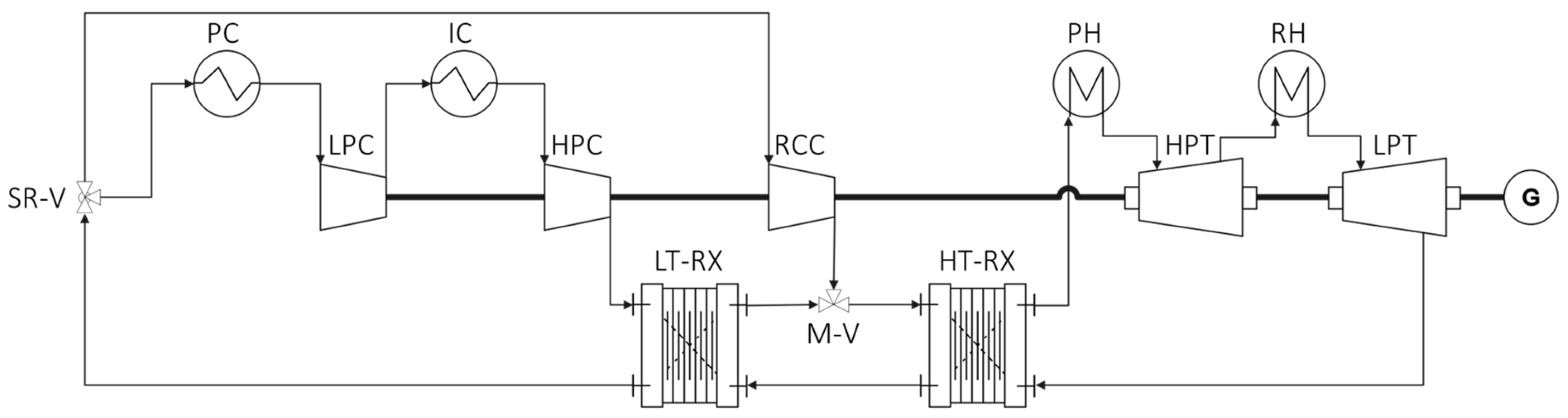
Figure 2.
Axial-turbine blade cascade.
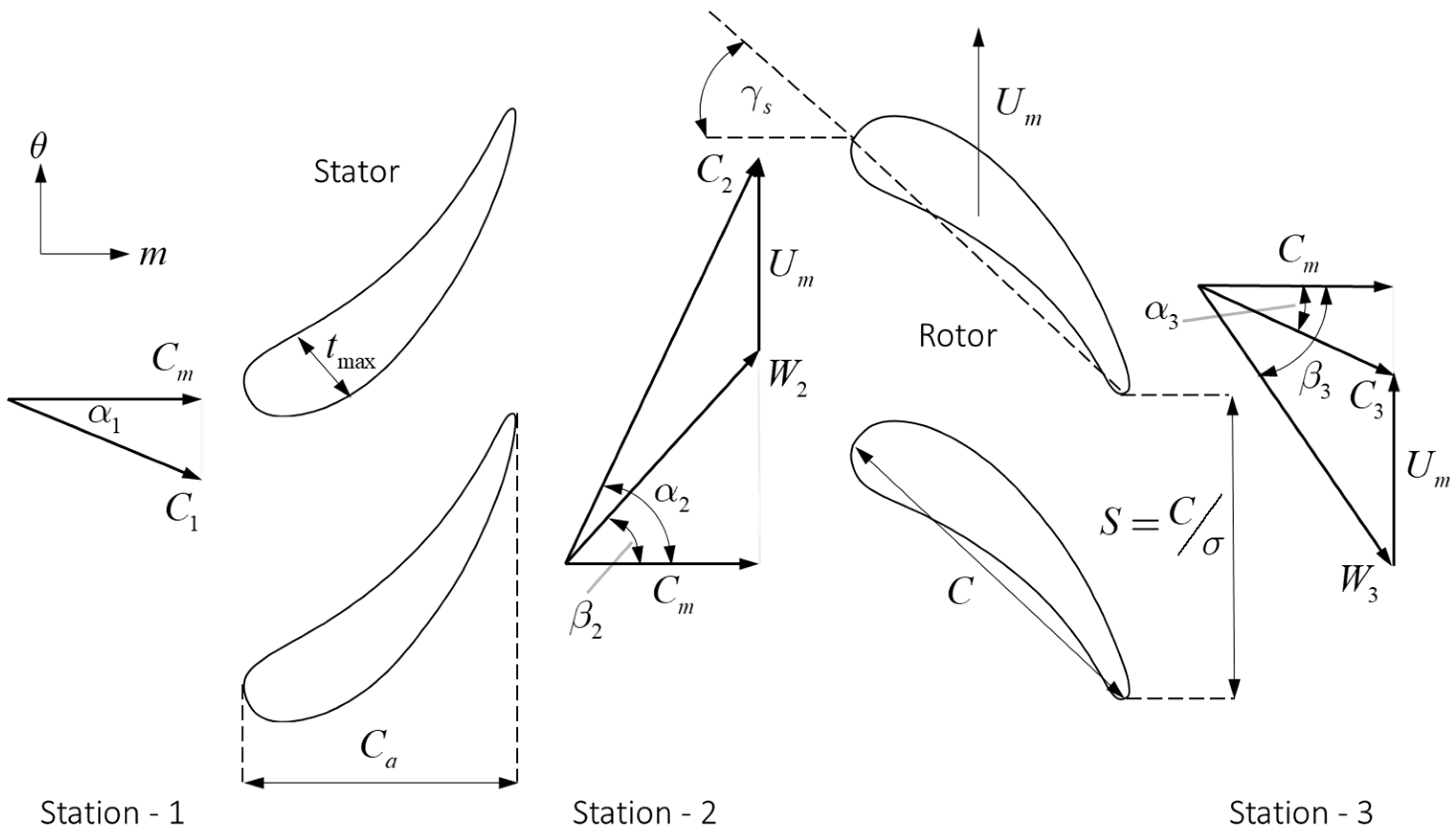
Figure 3.
Solution algorithm for mean line design.
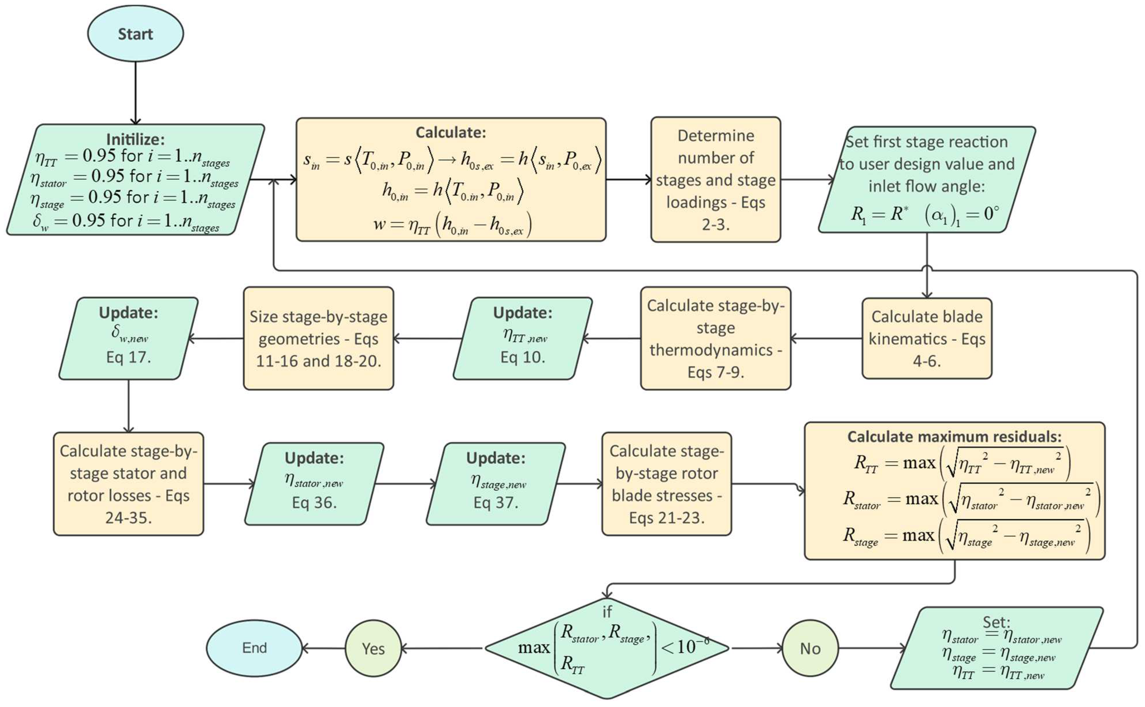
Figure 4.
Iso-surfaces for total-to-total isentropic efficiency for the high- and low-loading HPT designs.
Figure 4.
Iso-surfaces for total-to-total isentropic efficiency for the high- and low-loading HPT designs.
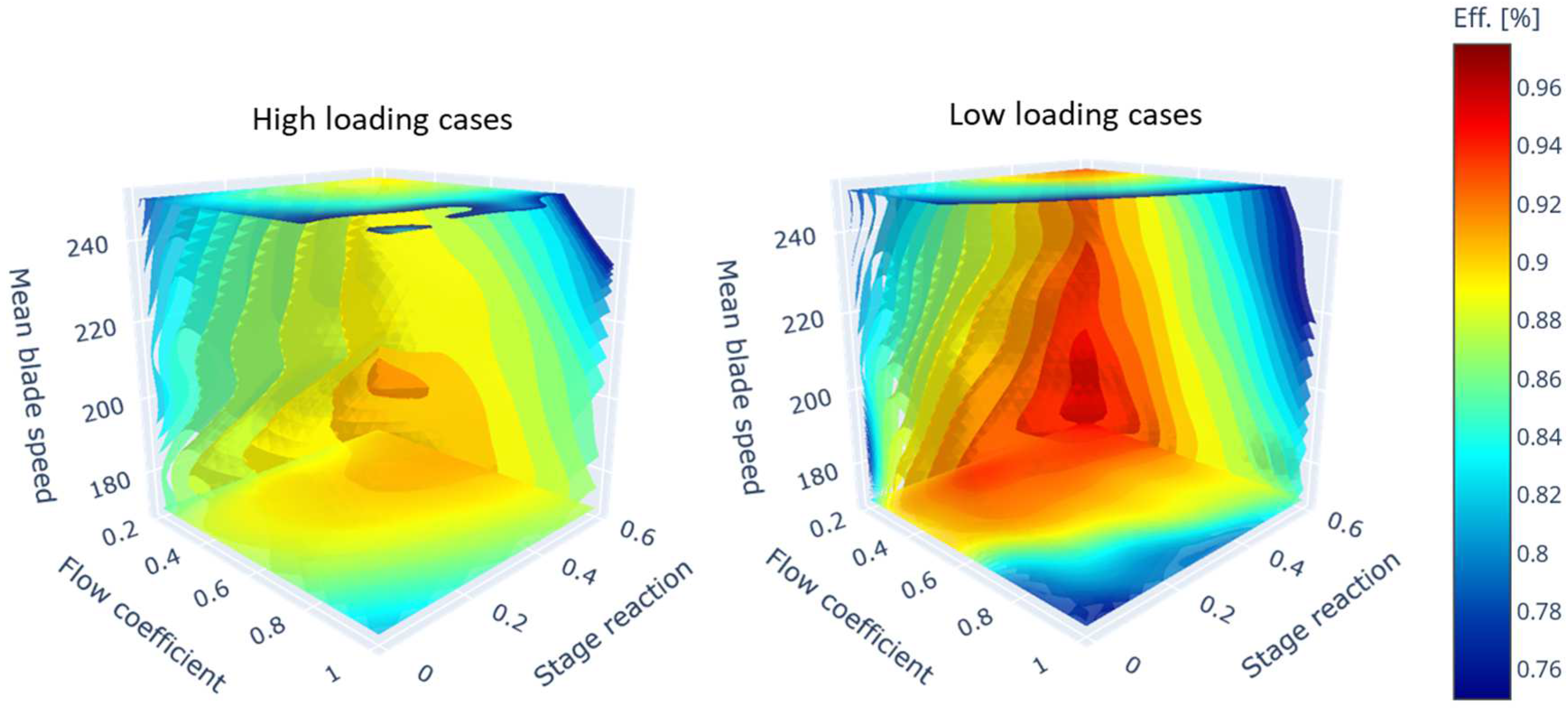
Figure 5.
Iso-surfaces for combined peak HPT rotor stress (top). Total-to-total isentropic efficiency as a function of peak rotor stresses (y-axis), mean rotor chord length (x-axis) and mean rotor blade height (marker size) for HPT designs (bot).
Figure 5.
Iso-surfaces for combined peak HPT rotor stress (top). Total-to-total isentropic efficiency as a function of peak rotor stresses (y-axis), mean rotor chord length (x-axis) and mean rotor blade height (marker size) for HPT designs (bot).
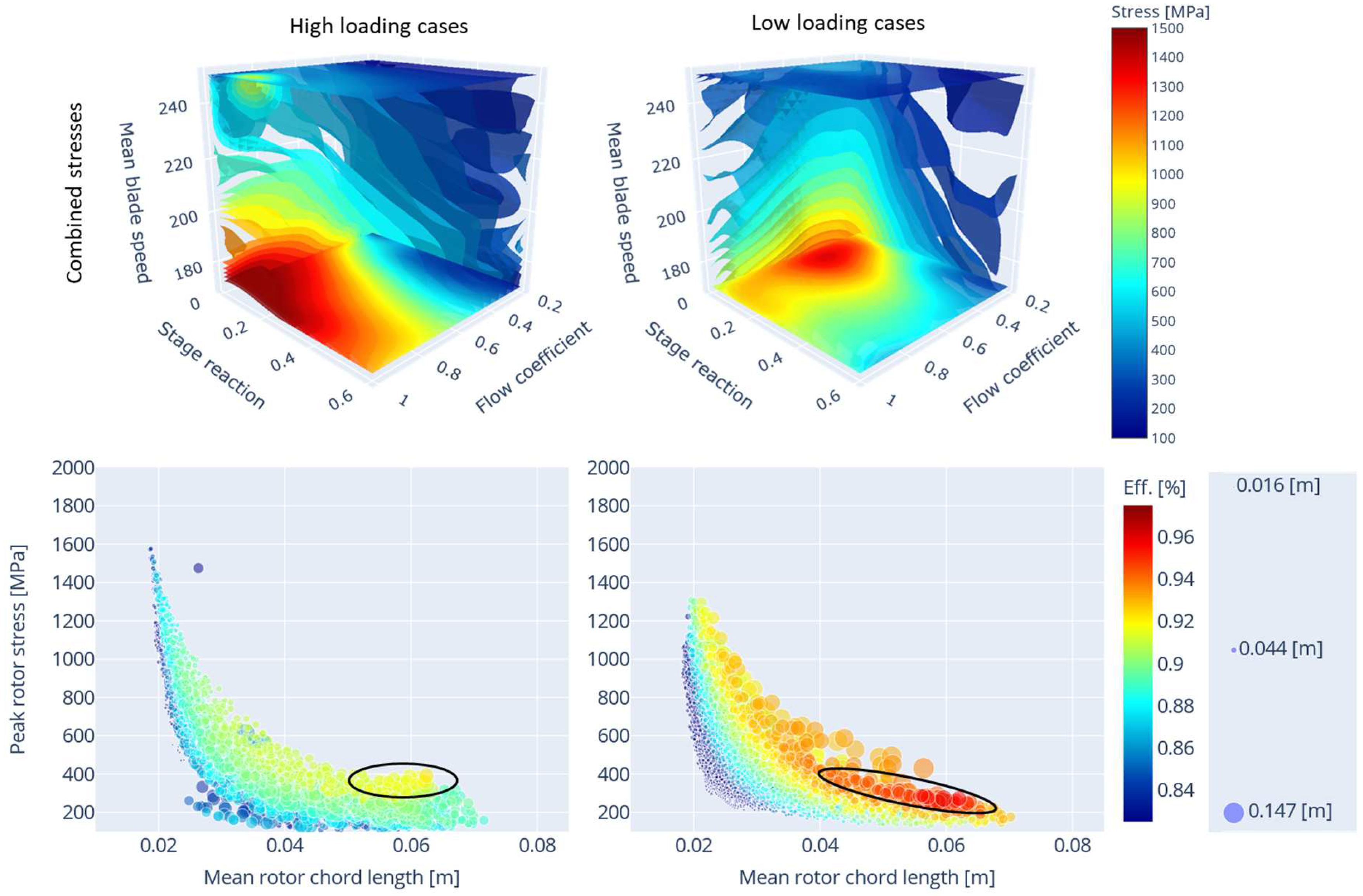
Figure 6.
Percentage contribution of gas bending stresses for HPT high- and low-loading designs.
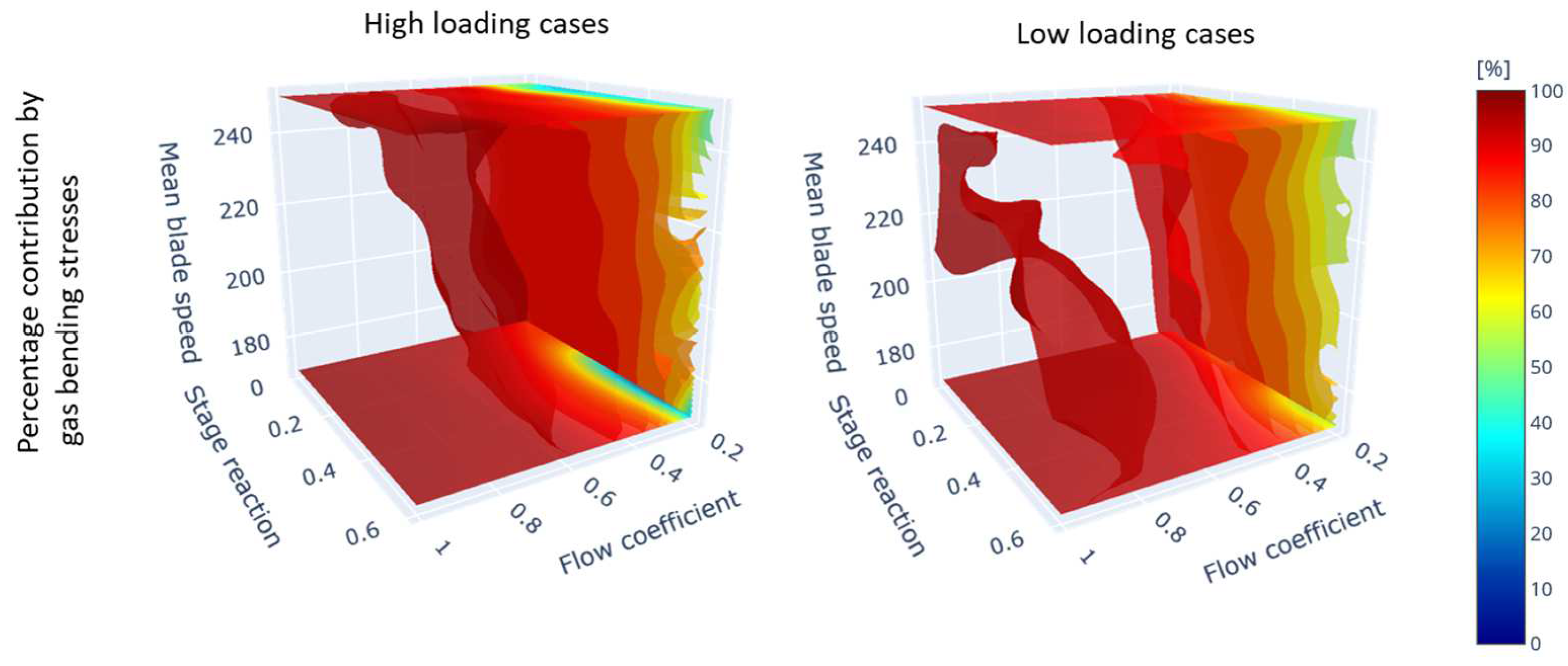
Figure 7.
Pareto fronts of non-dominating optimal solutions for HPT high- and low-loading designs showing total-to-total isentropic efficiency and peak combined rotor stress.
Figure 7.
Pareto fronts of non-dominating optimal solutions for HPT high- and low-loading designs showing total-to-total isentropic efficiency and peak combined rotor stress.
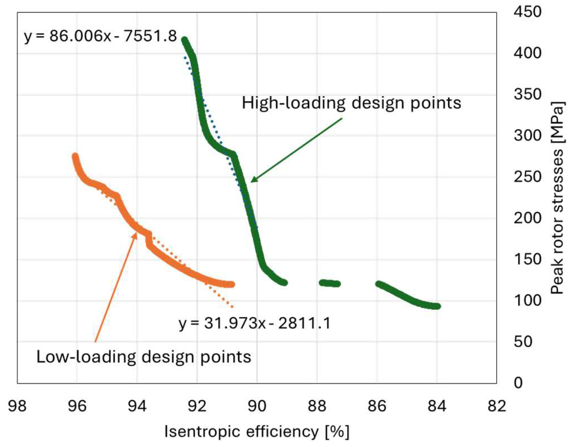
Figure 8.
Iso-surfaces for total-to-total isentropic efficiency for the high- and low-loading LPT designs.
Figure 8.
Iso-surfaces for total-to-total isentropic efficiency for the high- and low-loading LPT designs.
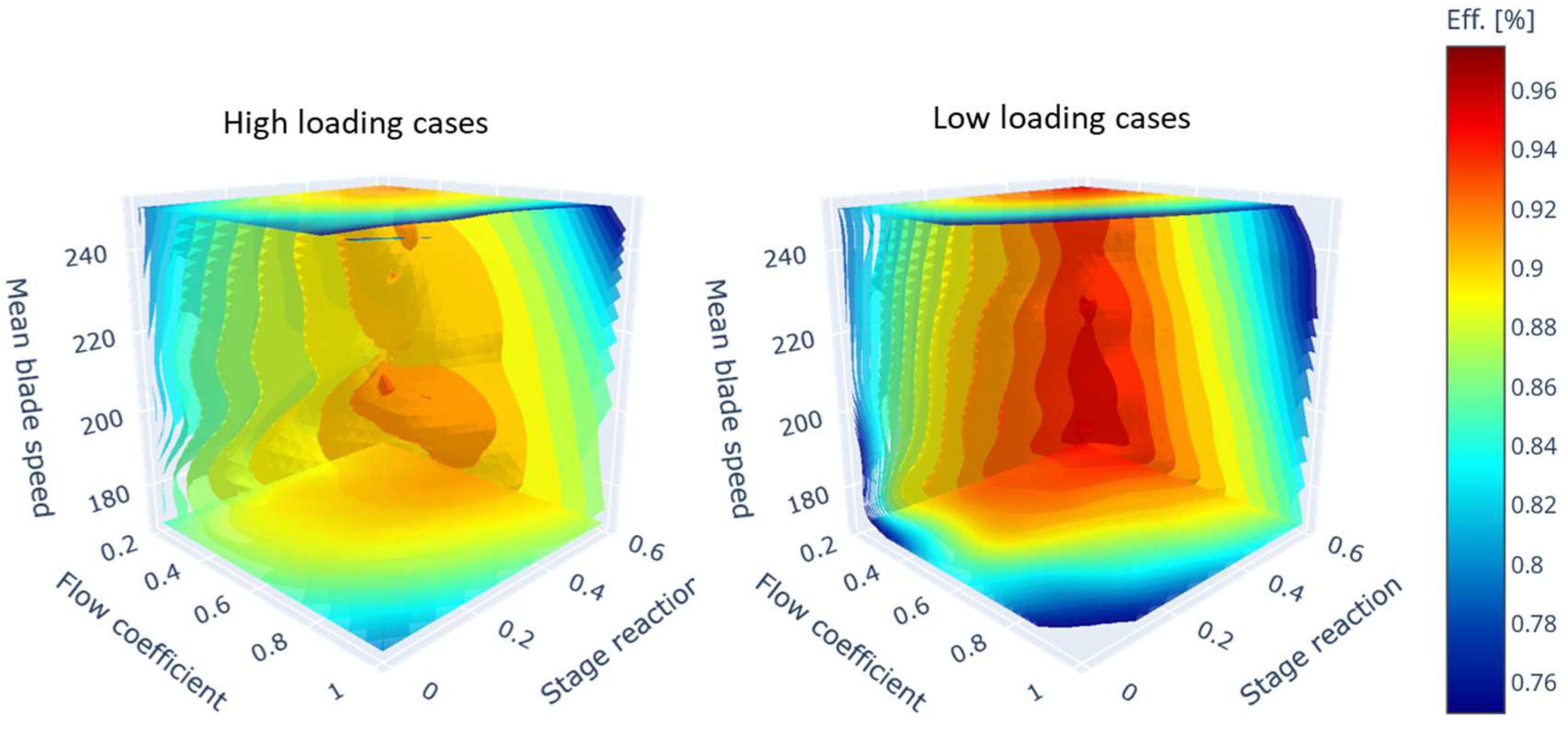
Figure 9.
Iso-surfaces for combined peak LPT rotor stress (top). Total-to-total isentropic efficiency as a function of peak rotor stresses (y-axis), mean rotor chord length (x-axis) and mean rotor blade height (marker size) for LPT designs (bot).
Figure 9.
Iso-surfaces for combined peak LPT rotor stress (top). Total-to-total isentropic efficiency as a function of peak rotor stresses (y-axis), mean rotor chord length (x-axis) and mean rotor blade height (marker size) for LPT designs (bot).
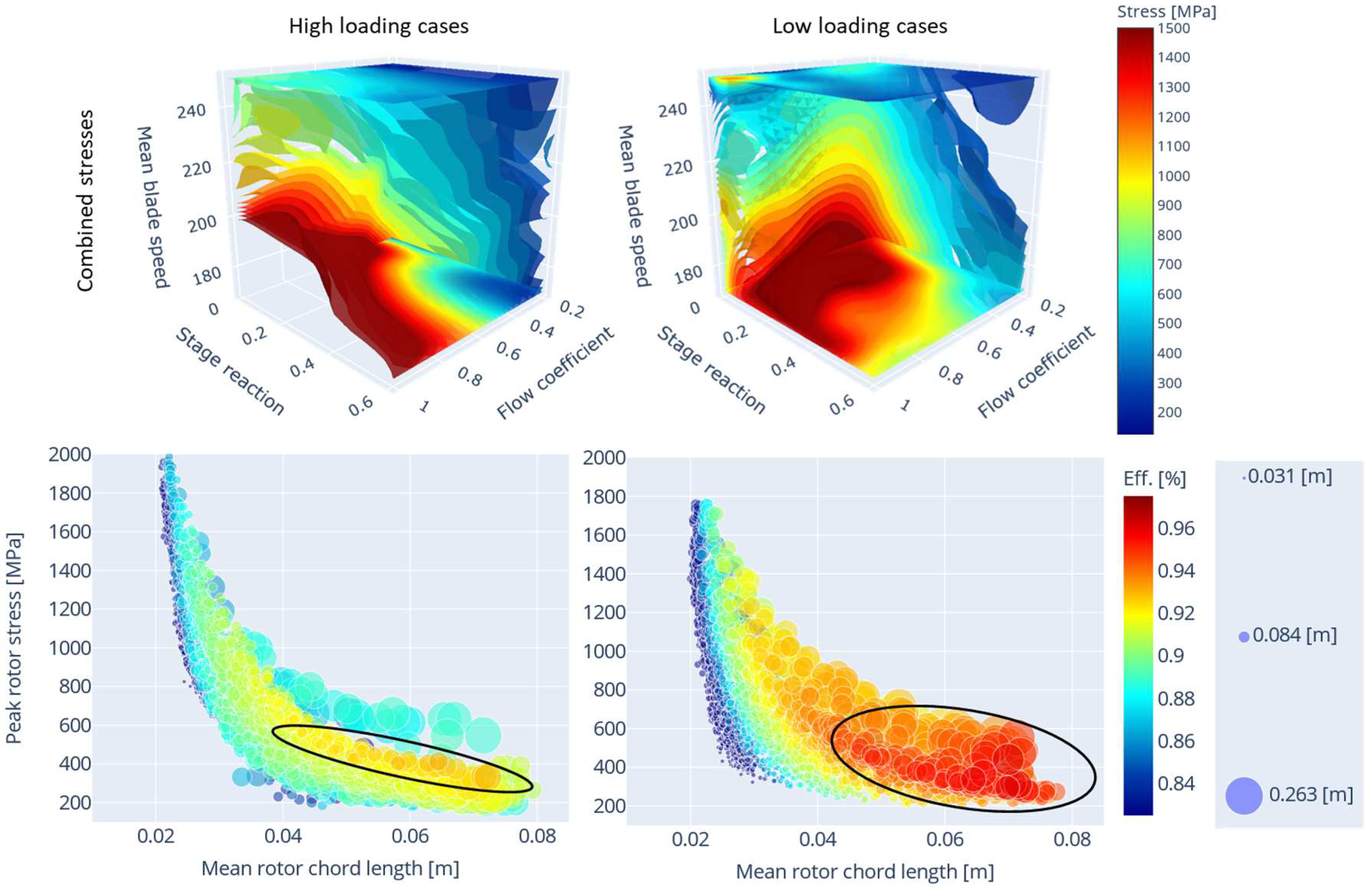
Figure 10.
Pareto front of non-dominating optimal solutions for LPT high- and low-loading designs showing total-to-total isentropic efficiency and peak combined rotor stress.
Figure 10.
Pareto front of non-dominating optimal solutions for LPT high- and low-loading designs showing total-to-total isentropic efficiency and peak combined rotor stress.
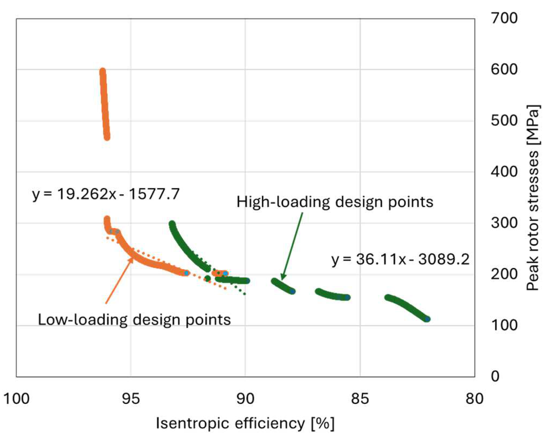
Figure 11.
Contours plots of relative Mach number in first and final stages of selected optimal high- and low-loading HPT machines at midplane.
Figure 11.
Contours plots of relative Mach number in first and final stages of selected optimal high- and low-loading HPT machines at midplane.
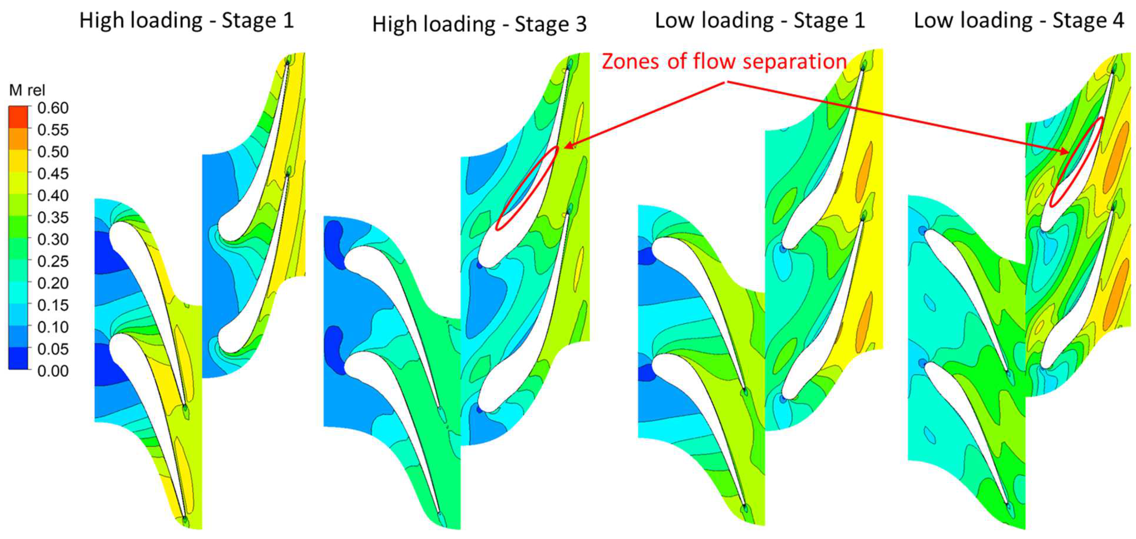
Figure 12.
Contours plots of relative Mach number in first and final stages of selected optimal high- and low-loading LPT machines at midplane.
Figure 12.
Contours plots of relative Mach number in first and final stages of selected optimal high- and low-loading LPT machines at midplane.


Table 1.
Design inputs for axial turbines.
| Parameters | HPT | LPT | Units |
|---|---|---|---|
| 823.15 | 823.15 | K | |
| 244.44 | 136.35 | bar(a) | |
| Mass flow rate, | 567 | 567 | kg/s |
| 1.754 | 1.754 | - | |
| 9000 | 9000 | rpm |
Table 2.
Typical axial turbine design parameter ranges from literature.
| Parameters | Values | Units |
|---|---|---|
| 0.0-0.6 [19] | - | |
| Flow coefficient, | 0.2-1.0 [5] | - |
| 0.4-1.5 [5] | - | |
| 180 [1] -187.6 [18] | m/s |
Table 3.
Results of selected HPT design criteria.
| Design scenarios | [-] | [-] | [m/s] | [-] | [%] | Volume [L] | [MPa] |
|---|---|---|---|---|---|---|---|
| - highest efficiency | 0.59 | 0.21 | 194.3 | 3 | 92.2 | 75 | 391 |
| - highest efficiency | 0.6 | 0.22 | 179.3 | 7 | 96.0 | 169 | 272 |
| - lowest combined peak rotor stress | 0.26 | 0.27 | 249 | 2 | 86.4 | 39 | 108 |
| - lowest combined peak rotor stress | 0.58 | 0.35 | 247.0 | 4 | 90.4 | 53 | 127 |
| - selected non-dominant optimal solution (min. distance from [0,0]) | 0.59 | 0.2 | 172.7 | 3 | 89.7 | 86 | 172 |
| - selected non-dominant optimal solution (min. distance from [0,0]) | 0.6 | 0.2 | 249.8 | 4 | 92.6 | 96 | 164 |
Table 4.
Results of selected LPT design criteria.
| Design scenarios | [-] | [-] | [m/s] | [-] | [%] | Volume [L] | [MPa] |
|---|---|---|---|---|---|---|---|
| - highest efficiency | 0.58 | 0.29 | 197.7 | 3 | 93.1 | 99 | 413 |
| - highest efficiency | 0.59 | 0.22 | 179.3 | 7 | 96.1 | 344 | 440 |
| - lowest combined peak rotor stress | 0.42 | 0.29 | 249.1 | 2 | 90.4 | 66 | 181 |
| - lowest combined peak rotor stress | 0.59 | 0.43 | 245.5 | 4 | 92.2 | 79 | 212 |
| - selected non-dominant optimal solution (min. distance from [0,0]) | 0.6 | 0.2 | 181.4 | 3 | 91.3 | 81 | 217 |
| - selected non-dominant optimal solution (min. distance from [0,0]) | 0.6 | 0.23 | 248.5 | 4 | 94.4 | 154 | 221 |
Table 5.
Selected geometric parameters for optimal turbine designs.
| Parameter | HPT high loading | HPT low loading | LPT high loading | LPT low loading |
|---|---|---|---|---|
| [⁰] | 77.5/53.9 | 71.6/12.7 | 77.5/53.7 | 69.2/14 |
| [⁰] | 100.2/22.8 | 22.9/7.63 | 97.3/14.9 | 23.9/8.6 |
| [mm/mm] | 3.8/4.6 | 1.4/1.8 | 5.3/6.3 | 2.2/2.7 |
| [mm/mm] | 4.8/5.7 | 1.9/2.4 | 6.5/7.5 | 2.9/3.5 |
| [mm] | 98.3/107.1 | 47/50.5 | 157.2/173.8 | 73.3/78.9 |
| [mm] | 131.6/141.4 | 65.4/68.9 | 213.2/228.2 | 103.2/109 |
| [mm] | 183.2 | 265.2 | 192.4 | 263.7 |
| First stage number of stator/rotor blades | 30/30 | 40/31 | 27/27 | 41/29 |
| Final stage number of stator/rotor blades | 37/27 | 30/29 | 35/23 | 30/26 |
Table 6.
CFD simulation predictions for pressure ratios and total-to-total isentropic efficiencies. Values in brackets taken from mean line code predictions).
Table 6.
CFD simulation predictions for pressure ratios and total-to-total isentropic efficiencies. Values in brackets taken from mean line code predictions).
| Turbine stage and loading | ||
|---|---|---|
| HPT high loading | 1.64 (1.754) | 90.9% (89.7%) |
| HPT low loading | 1.7 (1.754) | 93.7% (91.3%) |
| LPT high loading | 1.69 (1.754) | 94.1% (92.6%) |
| LPT low loading | 1.73 (1.754) | 95.1% (94.4%) |
Disclaimer/Publisher’s Note: The statements, opinions and data contained in all publications are solely those of the individual author(s) and contributor(s) and not of MDPI and/or the editor(s). MDPI and/or the editor(s) disclaim responsibility for any injury to people or property resulting from any ideas, methods, instructions or products referred to in the content. |
© 2025 by the authors. Licensee MDPI, Basel, Switzerland. This article is an open access article distributed under the terms and conditions of the Creative Commons Attribution (CC BY) license (http://creativecommons.org/licenses/by/4.0/).
Copyright: This open access article is published under a Creative Commons CC BY 4.0 license, which permit the free download, distribution, and reuse, provided that the author and preprint are cited in any reuse.


