
Submitted:
06 May 2025
Posted:
07 May 2025
You are already at the latest version
Abstract
Nowadays, significant efforts are made to develop technologies that can efficiently utilize clean energy sources in a sustainable manner. For this reason, supercritical carbon dioxide recompression Brayton cycles receive increased interest due to their combination of high efficiency and increased components compactness, characteris-tics that can assist the maximization of cycle performance and reduction of economic costs. At the present work, a thermoeconomic model of a 10 MW recompression cycle was developed. Initially, thermodynamic models of recompression cycle components such as heater, high and low temperature recuperators, cooler, turbines and com-pressors were developed in a Cape-Open free platform and the results were validated with data from open literature. For the modelling of components cost, open litera-ture-based cost models were used where the components cost was assessed as a function of the components’ main thermodynamic performance parameters such as power or conductance-area product taking also into account material-based correc-tions. At the next step, a parametric analysis was performed and the effect of pa-rameters such as split ratio, maximum cycle temperature and recuperators thermal effectiveness on the performance and cost of the recompression cycle was investi-gated facilitating the identification of the most promising combination of cycle and components characteristics. Finally, a dedicated cost function was derived through which the cost per net power of the recompession cycle could be assessed that could be used for future technoeconomic analyses.
Keywords:
Recompression cycle
; Recuperators
; Components purchase cost
; Supercritical carbon dioxide
; Cost function
1. Introduction
Nowadays, the worldwide dependence of power production to fossil fuels utilization can result to significant problems related with environmental pollution and global warming. This situation can be further intensified by the unpredictable nature of fossil fuel commercial prices leading to negative effects on economic growth sustainability. Thus, significant efforts are provided by engineers to develop advanced technologies that can efficiently exploit economically affordable clean energy sources. One of the best choices to achieve these goals is the utilization of renewable energy sources combined with advanced power cycles such as the supercritical carbon dioxide Brayton cycle.
The supercritical CO2 Brayton cycle combines some interesting characteristics such as: high compactness, higher efficiency and simpler cycle layout. It has higher efficiency than the ideal gas Brayton cycle and simpler system layouts with higher power density than similar Rankine cycle derivatives for equivalent conditions. Furthermore, the s-CO2 Brayton cycle can perform closer to Carnot’s efficiency limit and can operate with increased efficiency as the supercritical CO2 Brayton cycle benefits from the unique properties of s-CO2. These benefits can be achieved due to the extraordinary properties of carbon dioxide which, by being in supercritical state, exhibits liquid-like properties resulting in a reduction of the fluid compression required power and to a significant increase of the s-CO2 cycle efficiency. The main advantages of s-CO2 as working fluid [1, 2], and s-CO2 Brayton cycles are presented in Table 1, [3]:
As the s-CO2 Brayton cycle system operates above the critical point, the minimum cycle pressure is always higher than the one of any existing steam Rankine cycle or gas Brayton cycle. As a result, the fluid remains dense, the volumetric flow rate decreases and the fluid density is higher, leading to ~10 times smaller turbomachinery, leading to a reduction of the overall size of the power plant size, improved maintenance and reduced operational and installation capital costs [2, 4]. Furthermore, in a supercritical CO2 Brayton cycle its thermophysical properties values vary strongly above its supercritical point. Thus, the density values in this region remain high and similar to the ones of its liquid state but with low viscosity and friction values, which reduce significantly the work consumption of the compressor [1].
Supercritical CO2 Brayton cycles provide a significant thermal efficiency increase over traditional steam Rankine cycles. On the other hand, the pressure ratio of the sCO2 Brayton cycle is relatively small in relation to steam Rankine cycle while the turbine outlet temperature is relatively high. Thus, from a strictly thermodynamic point of view, a large amount of heat remains unexploited right after the turbine, that can be recuperated with specifically designed high performance heat recuperators to further increase the thermal efficiency of the s-CO2 Brayton cycle. Thus, the use of recuperation in the s-CO2 Brayton cycle can have a significant influence on thermal efficiency, so significant that it can be considered as mandatory in order to surpass even the 50% thermal efficiency threshold and as a result, the use of recuperators of high effectiveness values is of high prioritization.
The present work is focused on one of the most promising supercritical power cycles variants, the supercritical carbon dioxide Brayton recompression cycle which is presented in Figure 1. This advanced cycle is combining recuperation and recompression to achieve increased thermal efficiency and operates with carbon dioxide in supercritical state so as to take advantage of both liquid-like density and gas-like transport properties, allowing for compact, high-performance turbomachinery. The recuperation processes within the cycle are achieved with the use of two recuperators, the Low-Temperature Recuperator and the High-Temperature Recuperator, that facilitate the achievement of lower heat rejection losses in the cooler, higher thermal efficiency than comparable Rankine cycle-based systems and an overall more effective utilization of external heat sources such as solar power, natural gas or waste heat. The main cycle components and their operation are presented in Table 2.
2. Model Development
2.1. Thermodynamic Model
At the first step, thermodynamic models of the recompression cycle main components, such as heater, recuperators, cooler, turbines and compressors, were developed with the use of the free Cape-Open to Cape-Open COCO simulator platform [6] where the components model were created using the Excel Unit add-in [5]. The main details of the developed components are presented in Table 3. For the modelling of the thermophysical properties of carbon dioxide the Peng-Robinson [7] Equation of State was used.
The performance and cost of the heat exchangers (High Temperature Recuperator, Low Temperature Recuperator and Cooler) was estimated as a function of the overall conductance of the heat exchanger, U, the required heat surface area, A, and the logarithmic mean temperature difference, LMTD, of the hot and cold flows, [8]. More specifically, the UA of the heat exchanger, the conductance-area product, can be calculated from the thermal duty, , and the logarithmic mean temperature difference as presented in Equation 1 and assuming counter flow alignment between the two flow streams.
Since in this equation constant thermophysical are assumed, due to the significantly varying thermophysical properties of the supercritical CO2 recompression cycle in the heat exchangers (i.e. the Low Temperature Recuperator, the High Temperature Recuperator and the Cooler), discretized sub-models were necessary to be developed for these components, in order to sufficiently capture the variations of the thermophysical properties of the supercritical carbon dioxide.In these sub-models the heat exchange process was divided into a large number of internal stages with equal heat transfer per unit and the overall UA value of the heat exchange process was calculated as the sum of the respective UA values of the units of the sub-models. In the present work three sub-model discretization scenarios were applied, corresponding to 20, 50 and 100 units, providing a less than 1% difference in their respective calculated UA values when shifting from 50 to 100 units, which was the finally selected sub-model units’ number. This number also is aligned with the conclusions of the work of Weiland et al., [9], where the minimum selected number of discretization units should be at least 20.
2.2. Components Cost Model
The components cost model were based on the conclusions of the works of Weiland et al. [9] and are supported also by the conclusions of the works of Drennen and Lance, [8], and Carlson et al., [10]. The selected cost components models are presented in Table 4.
Each component cost model is developed in the form of Equations (2), (3) and (4)
and
and
where C is the component cost, SP is the scale parameter used for the cost scaling, α, b, c and d are component-dependent cost coefficients and fT is the temperature dependent correction function which is used to take into account the effect of high temperature material requirements on component cost. In this correction function is the maximum temperature of the component and corresponds to the point where thinner and more expensive materials become more cost effective than thicker low-cost stainless steels and is estimated at 550oC, as mentioned in Weiland et al., [9].
The average uncertainty of the cost model functions for these components is estimated at -30% to +35% approximately, based on Weiland et al., [9].
2.3. Validation of the Thermodynamic and the Component Costs Models
For the validation of the model, the open literature data presented in the works of Weiland et al. [9] and Drennen and Lance [8], presented in Table 5, were introduced to the developed COCO model in order to assess the model thermodynamic performance. The comparative results are presented in Table 6 and Table 7 where, as can be seen, the results of the thermodynamic COCO model were in close agreement in relation to the data from open literature.
For the validation of the modelling of the components cost, the literature-based cost models of the recompression cycle components of Table 1 were used. The components costs were assessed as a function of the components’ main thermodynamic performance parameters, such as the power or the conductance-area product, as previously calculated by the heat exchanger sub-models with the 100 units discretization, taking also into account material-based corrections based on the components’ maximum temperature level when necessary. At the next step, the components cost of the COCO model was calculated and compared in relation to the results presented in the work of Weiland et al., [9] where as it can be seen, the components net cost values and distribution were in close agreement, having an ~1.8% maximum per component difference and a ~0.65% average difference in the total cost of all the power plant main components, as presented in Table 8 and Figure 2 and Figure 3.
As it can be seen, the largest cost percentage is presented on the high temperature level components such as the Heater, the High Temperature Recuperator and the Turbine. The cost of lower temperature level components such as the Low Temperature Recuperator, the Main Compressor, the Recompressor and the Cooler follows while the cost of Motors, Generator and Gearbox is kept to relatively limited values.
It is important to be noted that all cost-components throughout this work are corresponding to USD$-2017 since the original data from Weiland et al. used this cost reference level as baseline using the average Chemical Engineering Plant Cost Index (CEPCI) for 2017. For the translation of these costs to current year USD cost levels the CECPI index can be applied following an approach similar to the one presented in the work of Weiland et al., [9], for which the CECPI index is 567.5.
3. Results of Parametric Analysis and Discussion
At the next step, a parametric analysis of the recompression cycle characteristics was performed and the effect of significant cycle parameters such as split ratio, maximum cycle temperature and high and low temperature recuperators thermal effectiveness on the technoeconomic performance of the supercritical carbon dioxide recompression cycle was investigated. The analysis of the results facilitated the identification of the most promising combination of the cycle characteristics in order to achieve the most beneficial combination of power generation and system components cost and also provided an insight in the components cost significance in relation to the applied thermodynamic conditions of the system.
3.1. Effect of Heater Maximum Temperature on Thermal Efficiency and Cost per Net Power
In order to investigate the effect of heater maximum temperature on the recompression cycle thermal efficiency and the components cost a parametric analysis using the developed COCO model was performed by varying the Heater maximum temperature from 823.15K to 1023.15K and by keeping all the other parameters and components characteristics the same as in the ~10 MW reference case described in Table 5 in Validation Case 1: Weiland et al. The results are presented in Figure 4 and Figure 5.
As it can be seen in Figure 4, the recompression cycle thermal efficiency increases almost linearly as the Heater maximum temperature increases from 39.7% (for 823.15K) to 48.0% (for 1023.15K). Furthermore, regarding the components cost per net power, presented in Figure 5, the components cost per net power remains relatively low from 823.15K to 923.15K with a local minimum being presented for 873.15K at ~1.9$/W. The maximum components cost per net power is presented or 1023.15K at ~3.0$/W. This behaviour can be mainly attributed to the relative increase of the cost of major cycle components as the Heater maximum temperature increases from 873.15K to 1023.15K and more specifically to the significant cost increase of the Heater, Turbine and High Temperature Recuperator components when operating in higher temperatures as presented in Figure 6 and Figure 7.
3.2. Effect of Split Ratio on Thermal Efficiency, Cost per Net Power ($/W) and Total Components Cost
In order to investigate the effect of split ratio recompression cycle thermal efficiency and the components cost a parametric analysis using the developed COCO model was performed by varying the split ratio from 0.4 to 0.9 and by keeping all the other parameters and components characteristics the same as in the ~10 MW reference case described in Table 5 in Validation Case 1: Weiland et al. The results are presented in Figure 8, Figure 9 and Figure 10.
As it can be seen in Figure 8, the recompression cycle thermal efficiency increases as the split ratio increases from ~41% (for split ratio equal to 0.4) to ~48.0% (for split ratio equal to 0.7) and then gradually decreases to ~44% (for split ratio equal to 0.9). Furthermore, regarding the components cost per net power, presented in Figure 9, the components cost per net power constantly decreases with increasing split ratio since the higher net power potential of the cycle, presented in Figure 10, compensates for the additional cost for larger components, presented in Figure 11, which yet might not be required for the selected nominal cycle power levels.
3.3. Effect of Varying Recuperators Effectiveness on Thermal Efficiency and Cost per Net Power
In order to investigate the effect of recuperators effectiveness on the recompression cycle thermal efficiency, the net power and the components cost a parametric analysis using the developed COCO model was performed by varying the recuperators effectiveness from 0.855 to 0.975 and by keeping all the other parameters and components characteristics the same as in the ~10 MW reference case described in Table 5 in Validation Case 1: Weiland et al. The results are presented in Figure 12, Figure 13 and Figure 14.
As it can be seen in Figure 12 and Figure 13, the increase of the recuperators effectiveness of both the High and the Low Temperature Recuperators has a positive effect on both thermal efficiency and the net power of the recompression cycle. More specifically, the cycle thermal efficiency and net power present their minimum values when the recuperators effectiveness have their minimum investigated values, i.e. 0.855, resulting in a ~38% thermal efficiency and ~9150kW net power for the recompression cycle. On the other hand, for the maximum investigated recuperators effectiveness values of 0.975, both the thermal efficiency and the net power are maximized with the thermal efficiency approaching ~47% and the net power of the cycle approaching ~9850kW. However, these increases are achieved with a disproportionate increase in the total components cost and as a result the total components cost per net power ($/W) is not presented for the maximum effectiveness values but for the relatively intermediate effectiveness values of 0.915 for both the High and the Low Temperature Recuperators, as presented in Figure 14 where the minimum total components cost per net power is ~2.89 $/W. This is a significant conclusion that should be taken into consideration during the design stages of a recompression power plant in order to avoid utilizating recuperators of extremely high performance which however present disproportionately high purchase cost, which does not necessarily justify their selection from an economic point of view.
Futhermore, as shown in Figure 15, Figure 16, Figure 17, Figure 18, Figure 19, Figure 20, Figure 21, Figure 22, Figure 23, Figure 24, Figure 25 and Figure 26, where the results of similar analyses for varying maximum Heater temperature are presented, practically in all cases the combination of recuperators effectiveness values of and results in achieving approximately the minimum value of cost per net power for the examined maximum heater temperature since for this combination of effectivenesses the cost per net value becomes minimum and almost constant near effectiveness 0.915 with only minor changes being noticed for the maximum Heater temperature of 1023.15K. Additionally, as it can be seen in Table 9 when the maximum Heater temperature takes relatively lower values, i.e. up to 923.15K, then the cost per net power remains relatively low since for these conditions the effect of maximum temperature on components cost remains still limited as most components operate below the 550oC threshold. This effect becomes significant after the maximum Heater temperature is equal to or more than 973.15K, resulting in a gradual cost per net power increase until 1023.15K, reaching the value of 2.85$/W.
3.4. Development of Cost Functions for Total Components Cost Taking into Account Recuperators Effectiveness and Heater Maximum Temperature
At the next step, the total components cost data which were included in Figure 5 and Figure 14, were combined in order to derive dedicated cost functions through which the total component cost of the recompression cycle could be estimated.
The applied approach was based on the following steps, following an approach similar to the one presented in international literature in the work of Salpingidou et al, [11].:
- 1)
- For all cases under investigation the total cost of the components was normalized with the respective total cost of the components corresponding to the ~10 MW reference case described in Table 5 in Validation Case 1: Weiland et al.
- 2)
- 3)
- For the data included in Figure 14, five (5) additional equations were derived, each one corresponding to a specific Low Temperature Recuperator effectiveness value, i.e. 0.855, 0.885, 0.915, 0.945 and 0.975, as presented in Equation (7):whereand the values of coefficients are presented in Figure 27, Figure 28, Figure 29, Figure 30 and Figure 31 where x indicates and y indicates .
- 4)
- For the derivation of a general cost function, all the values of coefficients for i=0.855, 0.995, 0.915, 0.945 and 0.975 were reprocessed in order to derive dedicated functions of their variation in relation to the variation of the High Temperature Recuperator effectiveness value, These values and these functions are presented in Table 10 and Figure 32, Figure 33, Figure 34 and Figure 35.
For the derivation of the general purchase cost function the accumulated effects of both Recuperators and maximum Heater temperature were included by using Equations (5) to (8), following an approach similar to the one of Salpingidou et al, [11]. This cost function is summarized in Equation (9) as follows:
where are polynomial functions of and are presented in Figure 32, Figure 33, Figure 34 and Figure 35. The comparison of this cost function with various data included in Figure 12, Figure 13, Figure 14, Figure 15, Figure 16, Figure 17, Figure 18, Figure 19, Figure 20, Figure 21, Figure 22, Figure 23, Figure 24, Figure 25, Figure 26, Figure 27, Figure 28, Figure 29, Figure 30, Figure 31, Figure 32, Figure 33, Figure 34, Figure 35 and Figure 36 is shown in Figure 36, presenting an average difference of ~1.0%.
4. Conclusions
Supercritical CO₂ Brayton Cycles appear as a compact and efficient technology that offers noticeable advantages over traditional steam Rankine and gas Brayton cycles since they benefit from convenient supercritical properties of CO₂, enabling smaller and possibly less expensive turbomachinery. The combination of supercritical CO2 as working fluid with recompression cycle layouts can significantly improves cycle efficiency by recovering more heat through two recuperators, i.e. the High Temperature and Low Temperature Recuperators, and by splitting the flow and recompressing a fraction without full cooling.
These characteristics result in increased interest and studies in the scientific community in order to conclude on the optimum recompression cycle operational characteristics targeting both thermodynamic and economic optimization. A large part of these attempts has been performed with the use of numerical tools modelling both thermodynamic and economic aspects of the system. Such an effort was performed at the present work where a thermoeconomic model of a recompression cycle of 10MW reference nominal power was developed in order to assess both the thermodynamic performance and the cycle components purchase cost in relation to significant recompression cycle parameters such as split ratio, maximum cycle temperature and high and low temperature recuperators thermal effectiveness.
For these reasons, a detailed, component-by-component thermodynamic model was developed using the free Cape-Open to Cape-Open COCO simulator and its customizable Excel add-in, while for the accurate modelling of the s-CO2 thermophysical properties the Peng-Robinson Equation of State was used. In addition, for the modelling of the components cost, dedicated literature-based cost models of the recompression cycle components were applied where the component costs were assessed as scaled functions of the components main thermodynamic performance parameters. More specifically, detailed sub-models were developed for the proper refinement and discretization of the recompression cycle heat exchangers, i.e. High and Low Temperature Recuperators and Cooler, in order to properly resolute the heat exchange process and accurately capture the variations of the s-CO2 thermophysical properties. In the present analysis three sub-model discretization scenarios were used, corresponding to 20, 50 and 100 units respectively, resulting in a less than 1% difference in the calculated UA values of the components, when shifting from 50 to 100 units, ensuring the accurate estimation of the heat exchanger components thermodynamic size and their accurate cost modelling. Both the model's thermodynamic and cost predictions aligned in close agreement with open literature published data having an ~1.8% maximum per component difference and a ~0.65% average difference in the total cost of all the power plant main components.
Furthermore, a detailed parametric analysis was performed where the effect of significant recompression cycle parameters on thermal efficiency, net power and cost per net power was assessed covering a wide range of conditions. The analysis of the results facilitated the identification of the most promising combination of cycle and components characteristics, especially regarding the recuperators effectiveness which were found to be more beneficial near the value of 0.915, in order to achieve the most beneficial combination of power generation and system components cost in relation to the thermodynamic conditions of the system, resulting in the minimum cost per net power value.
Finally, a dedicated cost function was derived through which the cost per net power of the recompression cycle could be assessed as a function of the Heater maximum temperature and the High and Low Temperature Recuperators effectiveness values. This derived cost function is planned to be used in near future for technoeconomic analysis of similar setups in order to assess the recompression cycle thermodynamic and cost characteristics for a wider design space of cycle operational parameters and components characteristics incorporating also additional parameters such as the effect of pressure ratio and the effect of cooler conditions, targeting the development of a more general thermoeconomic cost function for s-CO2 recompression cycles.
Author Contributions
Conceptualization, C.P.; methodology, C.P. and D.M.; software, D.M.; validation, C.P. and D.M.; formal analysis, C.P. and D.M.; investigation, C.P. and D.M.; writing—original draft preparation, C.P. and D.M.; writing—review and editing, C.P. and D.M.; visualization, C.P. and D.M.; supervision, C.P. and D.M.. All authors have read and agreed to the published version of the manuscript.
Funding
This research received no external funding.
Data Availability Statement
Data are contained within the article.
Acknowledgments
Not applicable.
Conflicts of Interest
The authors declare no conflicts of interest.
Abbreviations
The following abbreviations are used in this manuscript:
| English letters | |
| A | Heat transfer area |
| C | Component cost |
| CCF_LTR_i | Component Cost correction Function for Low Temperature Recuperator i |
| CCF_Tmax | Component Cost Function in relation to maximum heater temperature |
| CECPI | Chemical Engineering Plant Cost Index |
| CSP | Concentrated Solar Power |
| DP | Pressure drop |
| fT | Temperature dependent correction factor |
| HEX_HT_REC | High Temperature Recuperator |
| HEX_LT_REC | Low Temperature Recuperator |
| High_Temperature_HEX | High Temperature Recuperator |
| LMTD | Logarithmic mean temperature difference |
| Low_Temperature_HEX | Low Temperature Recuperator |
| Nc | Compressor isentropic efficiency |
| Nt | Turbine isentropic efficiency |
| P | Static pressure |
| Thermal duty | |
| s-CO2 | Supercritical carbon dioxide |
| SP | Scale parameter for cost |
| Material limit temperature | |
| Maximum temperature of component | |
| Maximum heater temperature | |
| U | Overall conductance of heat exchanger |
| UA | Conductance-area product |
| UA_HEX_HT_REC | Conductance-area product of High Temperature Recuperator |
| UA_HEX_LT_REC | Conductance-area product of Low Temperature Recuperator |
| Greek letters | |
| εHTR | High Temperature Recuperator effectiveness |
| εLTR | Low Temperature Recuperator effectiveness |
References
- Siddiqui, M.E.; Almitani, K.H. . Energy Analysis of the S-CO2 Brayton Cycle with Improved Heat Regeneration, Processes, 2018; 7, Article 3. [CrossRef]
- Atinga, K.A. Simulation Modelling and Techno-Economics of Supercritical Carbon Dioxide Recompression Closed Brayton Cycle, Energy and Power Engineering, 2024; 16, 325-344. [CrossRef]
- AHN, Y.; BAE, S. J.; KIM, M.; CHO, S. K.; BAIK, S.; LEE, J.I.; CHA, J.E. , REVIEW OF SUPERCRITICAL CO2 POWER CYCLE TECHNOLOGY AND CURRENT STATUS OF RESEARCH AND DEVELOPMENT, Nucl. Eng. Te c h n o l. 2 0 1 5; 4 7, 6 4 7 -6 6 1. [CrossRef]
- Mendez, C.; Rochau, G. . sCO2 Brayton Cycle: Roadmap to sCO2 Power Cycles NE Commercial Applications (SAND2018-6187), 2018; Sandia National Lab.
- amsterCHEM Excel CAPE-OPEN Unit Operation. Available online: https://www.amsterchem.com/excelunitop.html (accessed on 24 April 2025).
- COCO - the CAPE-OPEN simulator. Available online: https://www.cocosimulator.org/index.html (accessed on 24 April 2025).
- Peng, D. Y.; Robinson, D. B. . A New Two-Constant Equation of State, Industrial and Engineering Chemistry: Fundamentals, 1976; 15, 59–64. S2CID98225845. [CrossRef]
- Drennen, T. E.; Lance, B.W. An Integrated Techno-economic Modeling Tool for sCO2 Brayton Cycles, 2019; SANDIA REPORT, SAND2019-8738. [CrossRef]
- Weiland, N.T.; Lance, B.W.; Pidaparti, S.R. sCO2 Power Cycle Component Cost Correlations From DOE Data Spanning Multiple Scales and Applications, In Proceedings of the ASME Turbo Expo 2019: Turbomachinery Technical Conference and Exposition. Volume 9: Oil and Gas Applications; Supercritical CO2 Power Cycles; Wind Energy. 2019; Phoenix, Arizona, USA. June 17–21, V009T38A008. ASME. [CrossRef]
- Carlson, M.D.; Middleton, B.M.; Ho, C.K. Techno-Economic Comparison of Solar-Driven SCO2 Brayton Cycles Using Component Cost Models Baselined With Vendor Data and Estimates, In Proceedings of the ASME 2017 11th International Conference on Energy Sustainability collocated with the ASME 2017 Power Conference Joint With ICOPE-17, the ASME 2017 15th International Conference on Fuel Cell Science, Engineering and Technology, and the ASME 2017 Nuclear Forum, ASME 2017 11th International Conference on Energy Sustainability, 2017; Charlotte, North Carolina, USA. June 26–30, V001T05A009. ASME. [CrossRef]
- Salpingidou, C.; Misirlis, D.; Vlahostergios, Z.;, Flouros, M.;, Donus, F.;, Yakinthos, K. Design Optimization of Heat Exchangers for Aero Engines With the Use of a Surrogate Model Incorporating Performance Characteristics and Geometrical Constraints, In Proceedings of the ASME Turbo Expo 2018: Turbomachinery Technical Conference and Exposition, 2018; Volume 5C: Heat Transfer, Oslo, Norway. June 11–15. V05CT22A004. ASME. [CrossRef]
Figure 1.
The supercritical carbon dioxide Brayton recompression cycle as implemented in COCO simulator with the use of Excel Units Add-on custom programming, [5].
Figure 1.
The supercritical carbon dioxide Brayton recompression cycle as implemented in COCO simulator with the use of Excel Units Add-on custom programming, [5].
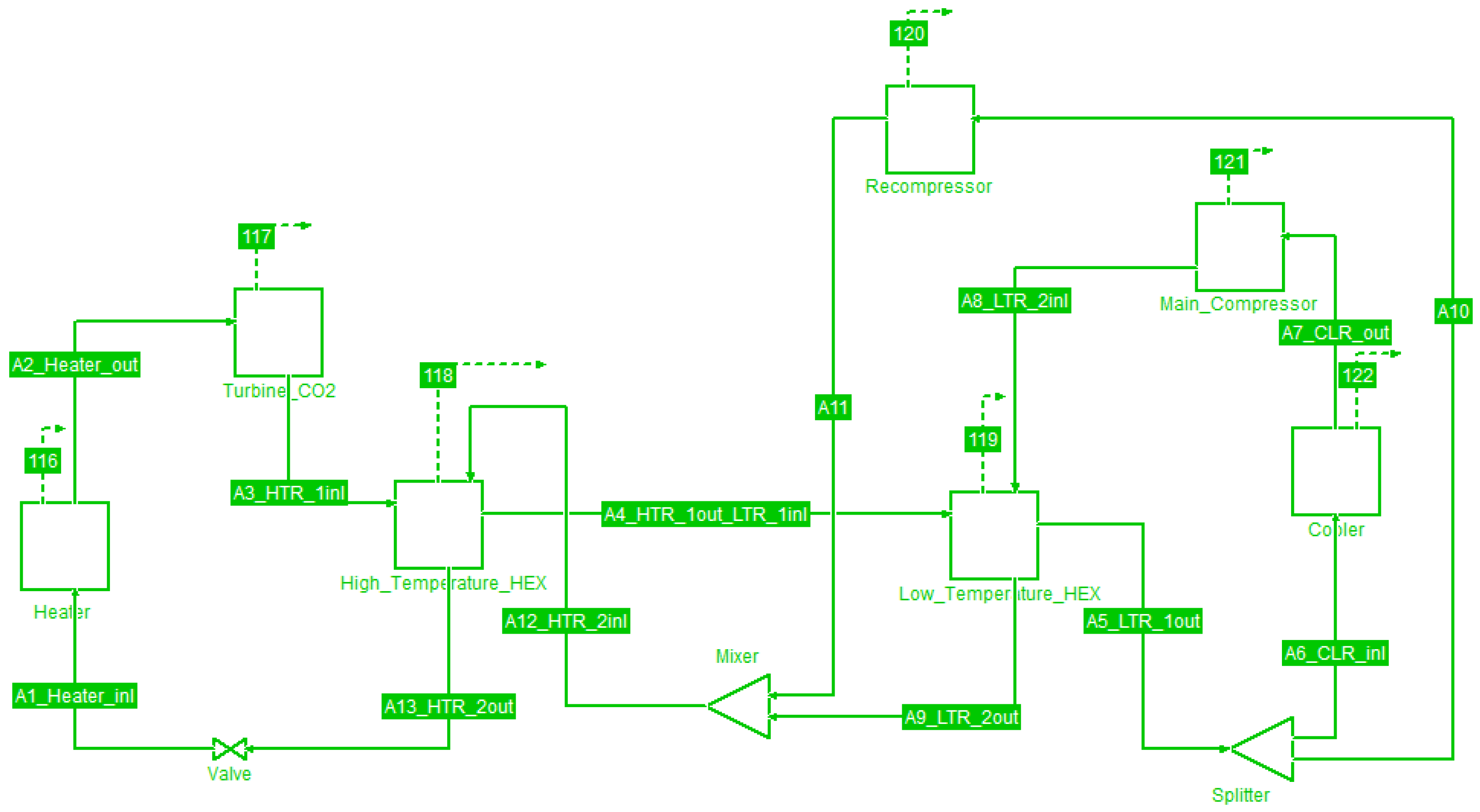
Figure 2.
Comparison of components cost between COCO model and Validation Case1 (Weiland et al., [9]).
Figure 2.
Comparison of components cost between COCO model and Validation Case1 (Weiland et al., [9]).
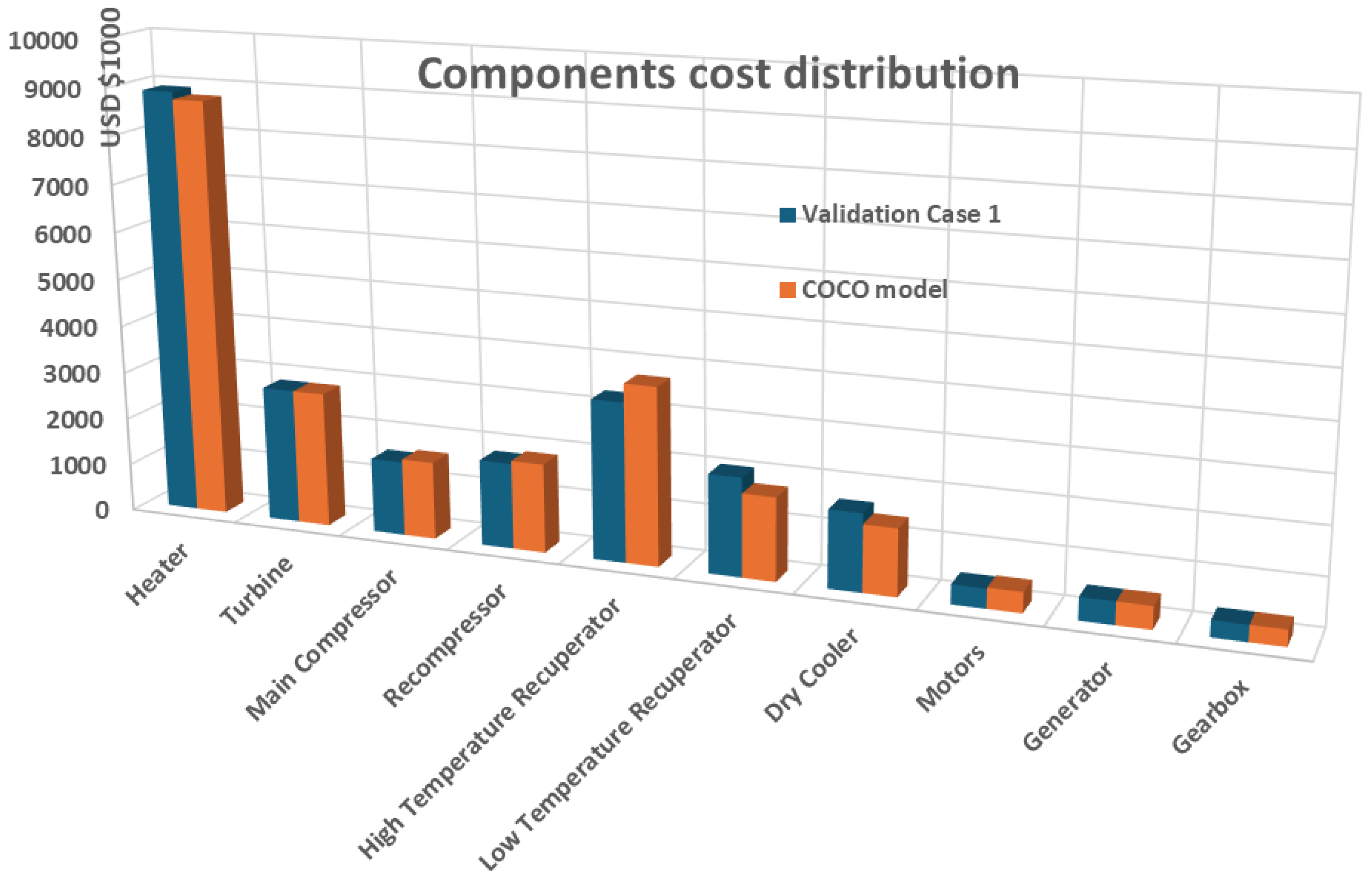
Figure 3.
Comparison of components cost % distribution between COCO model and Validation Case 1 (Weiland et al., [9]).
Figure 3.
Comparison of components cost % distribution between COCO model and Validation Case 1 (Weiland et al., [9]).
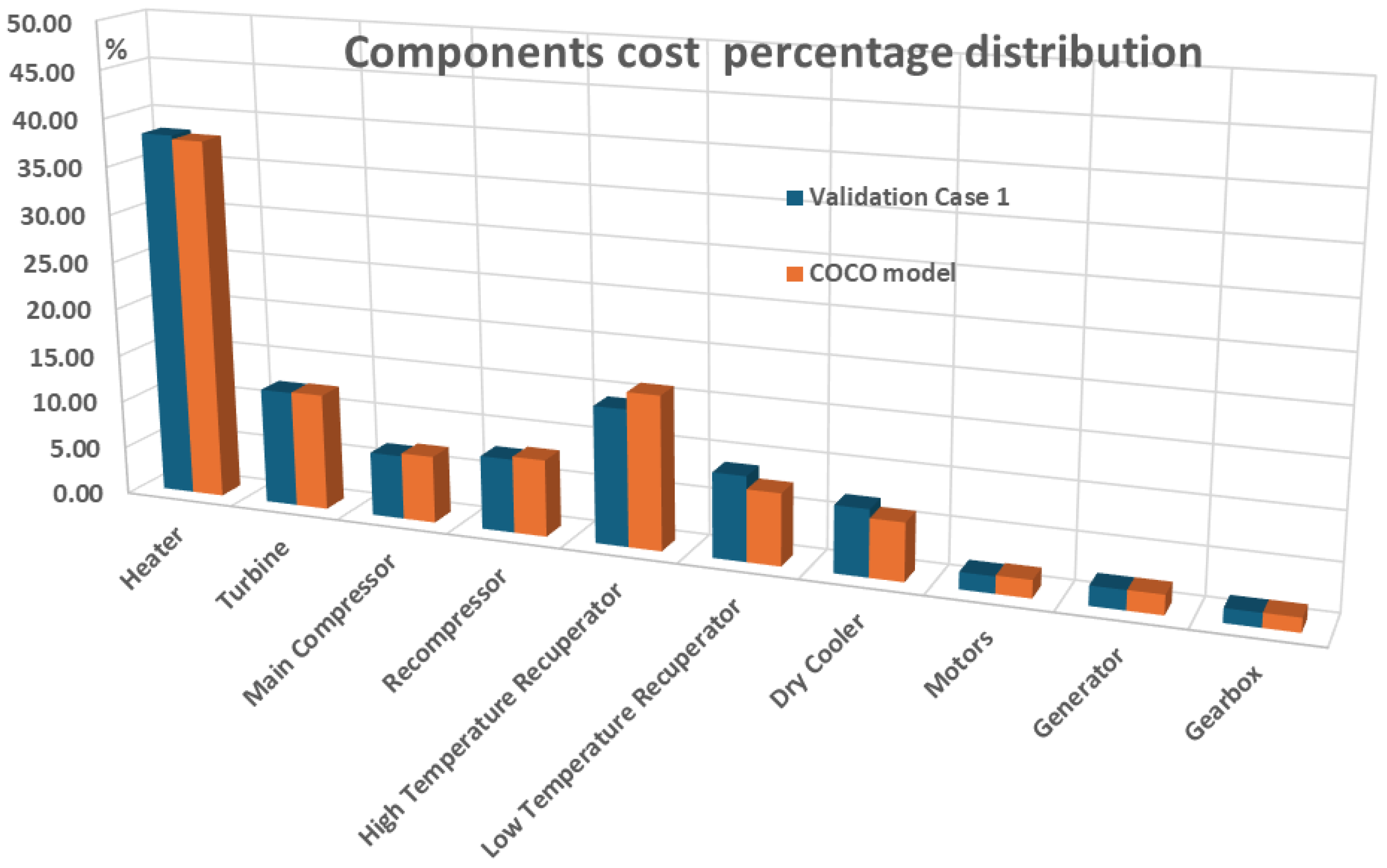
Figure 4.
Recompression cycle thermal efficiency vs heater maximum temperature.
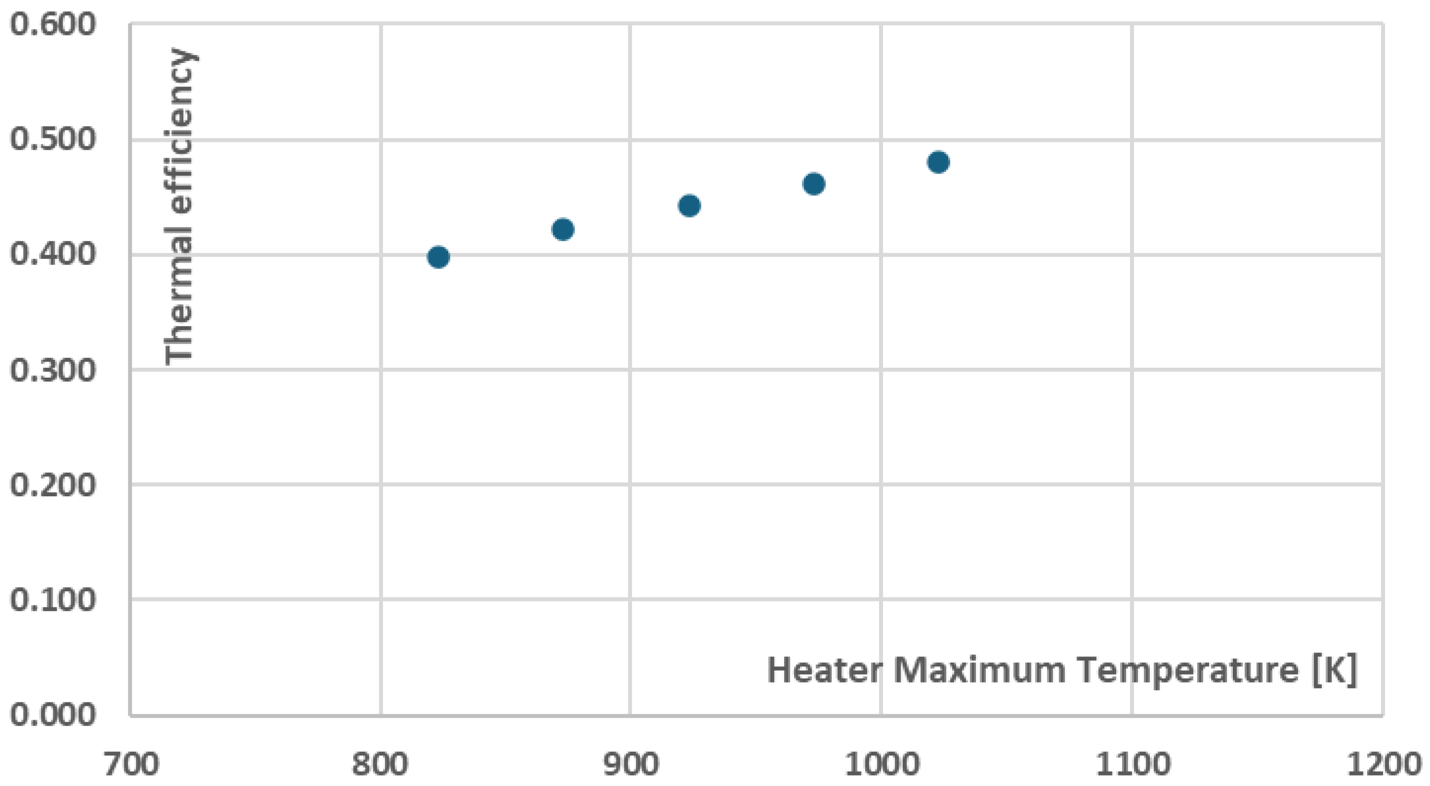
Figure 5.
Recompression cycle cost per net power with varying heater maximum Temperature.
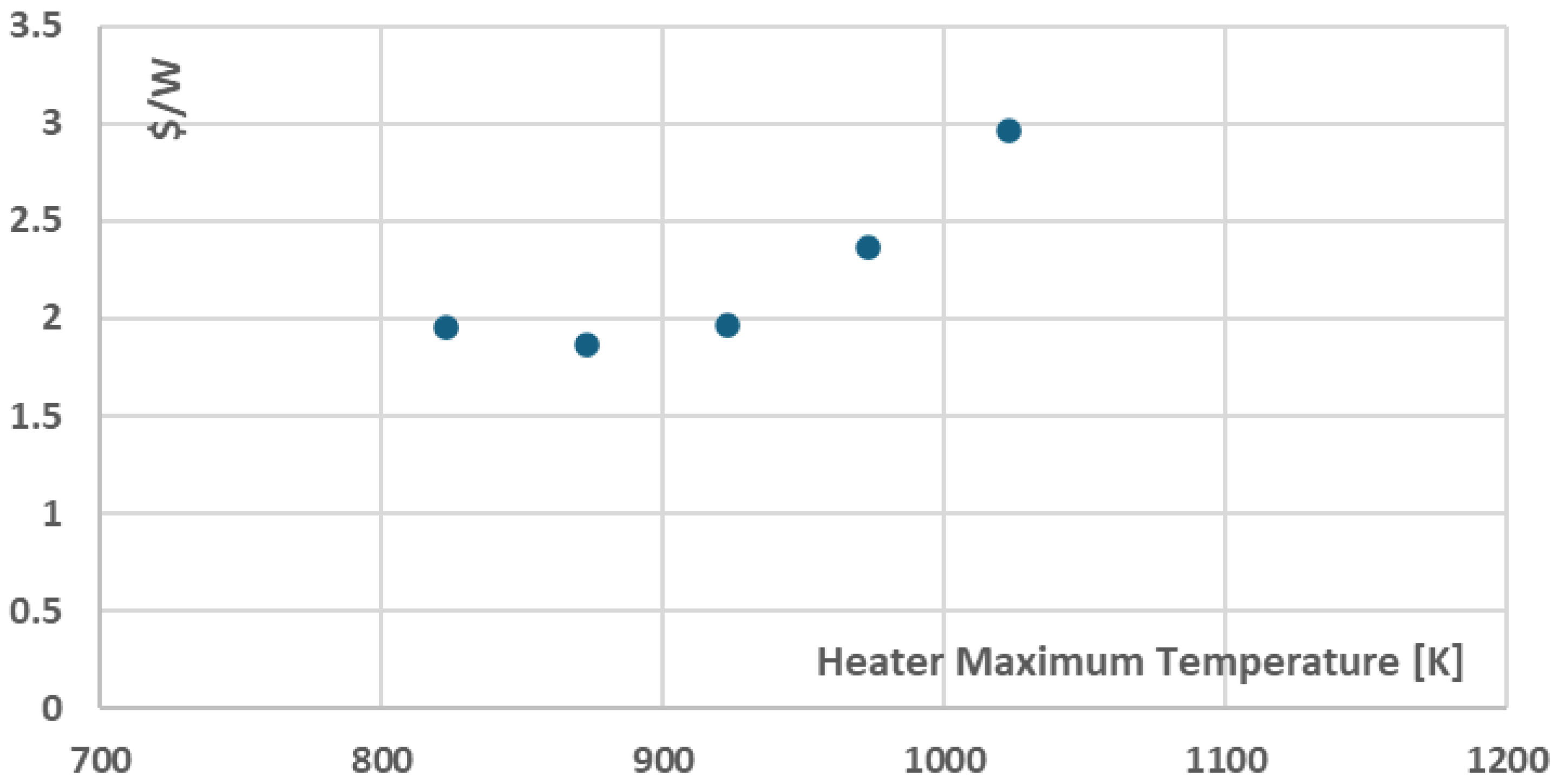
Figure 6.
Effect of varying Heater maximum temperature on recompression cycle main components cost.
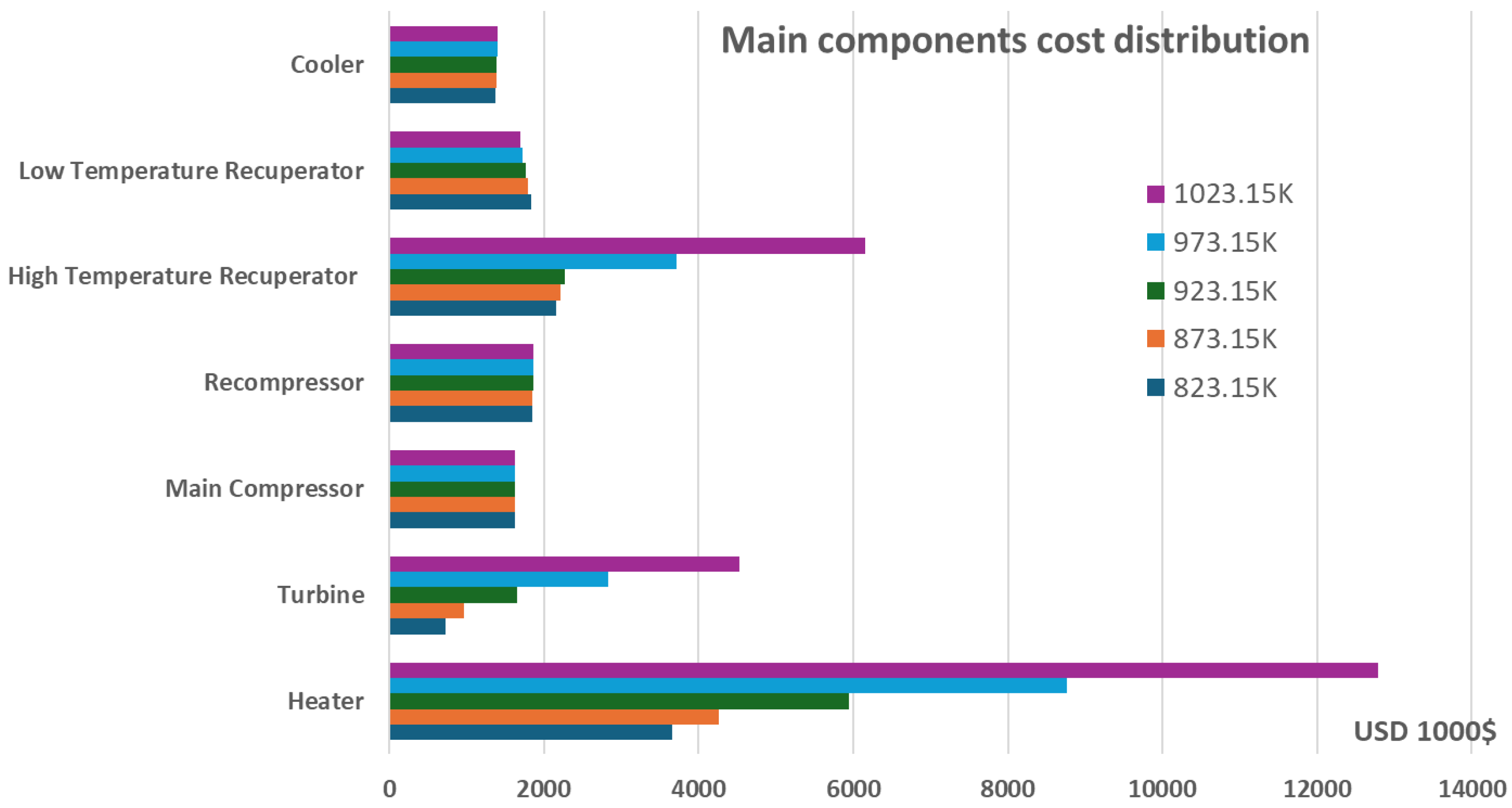
Figure 7.
Effect of varying Heater maximum temperature on recompression cycle main components cost distribution.
Figure 7.
Effect of varying Heater maximum temperature on recompression cycle main components cost distribution.
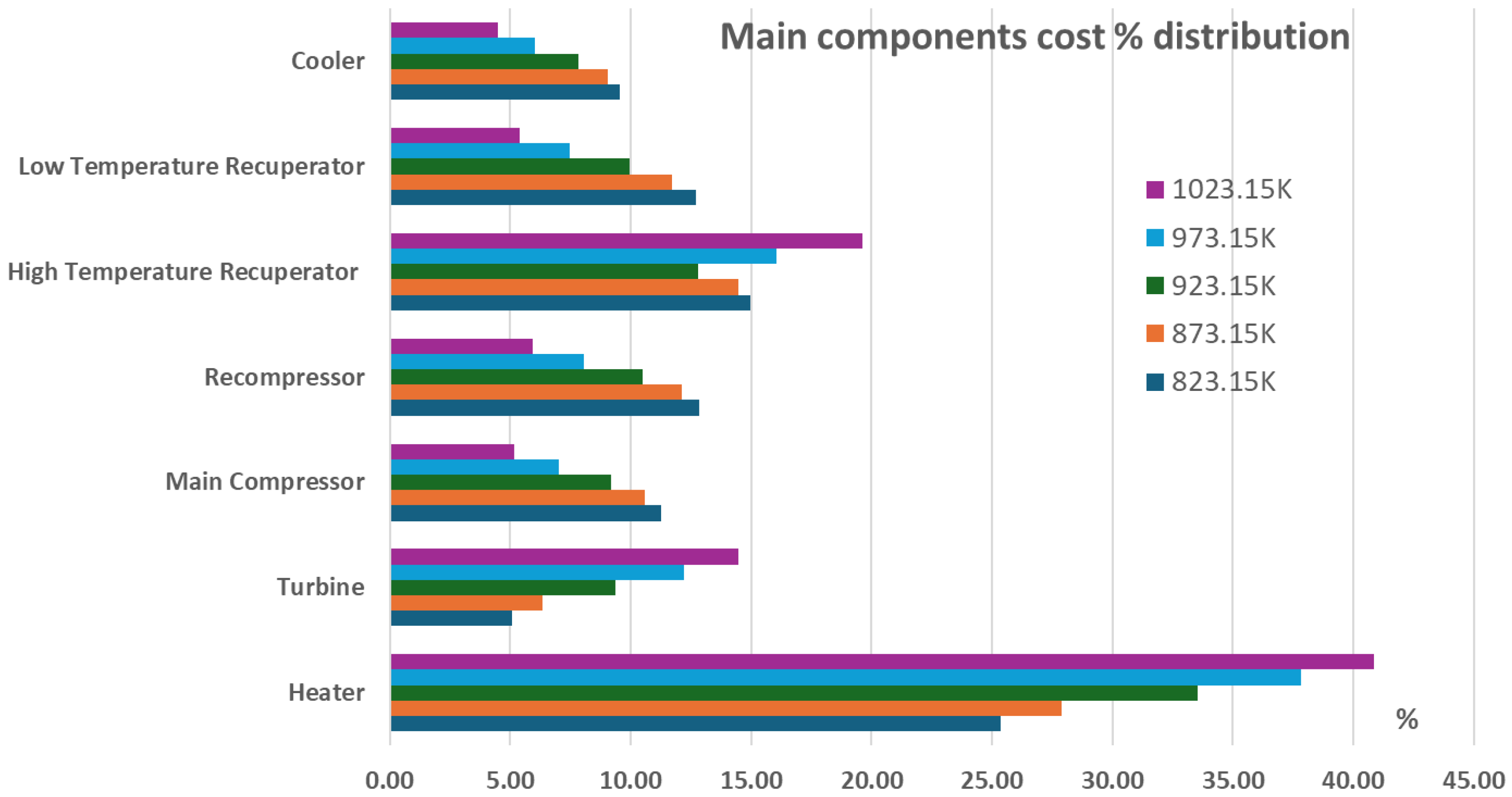
Figure 8.
Recompression cycle thermal efficiency with varying recompression split ratio.
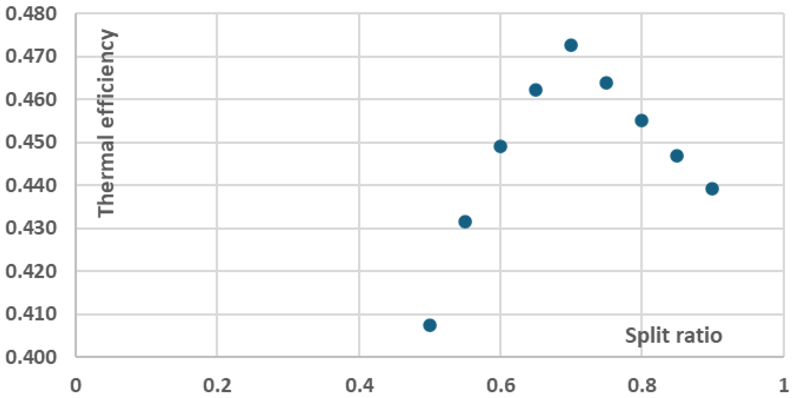
Figure 9.
Recompression cycle cost per net power with varying recompression split ratio.
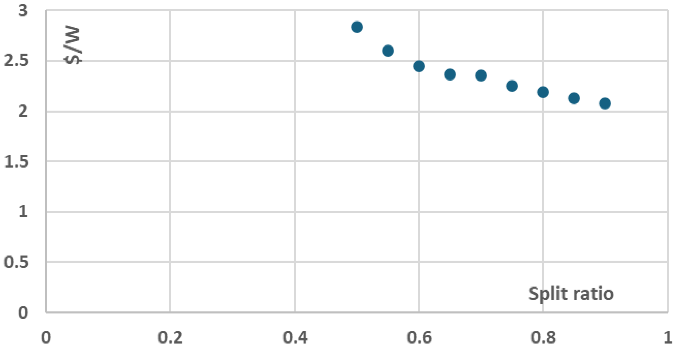
Figure 10.
Recompression cycle net power with varying recompression split ratio.
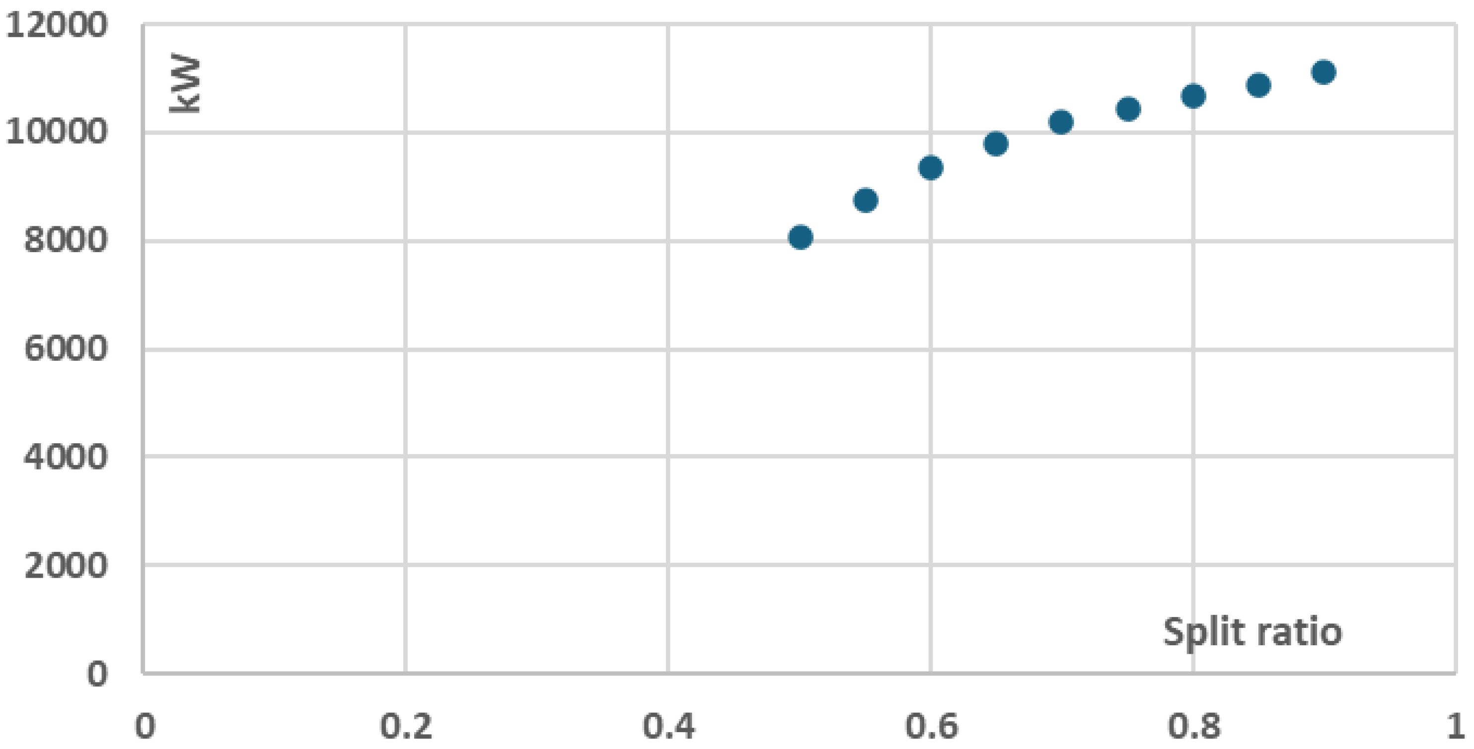
Figure 11.
Recompression cycle cost main components distribution with varying recompression split ratio.
Figure 11.
Recompression cycle cost main components distribution with varying recompression split ratio.
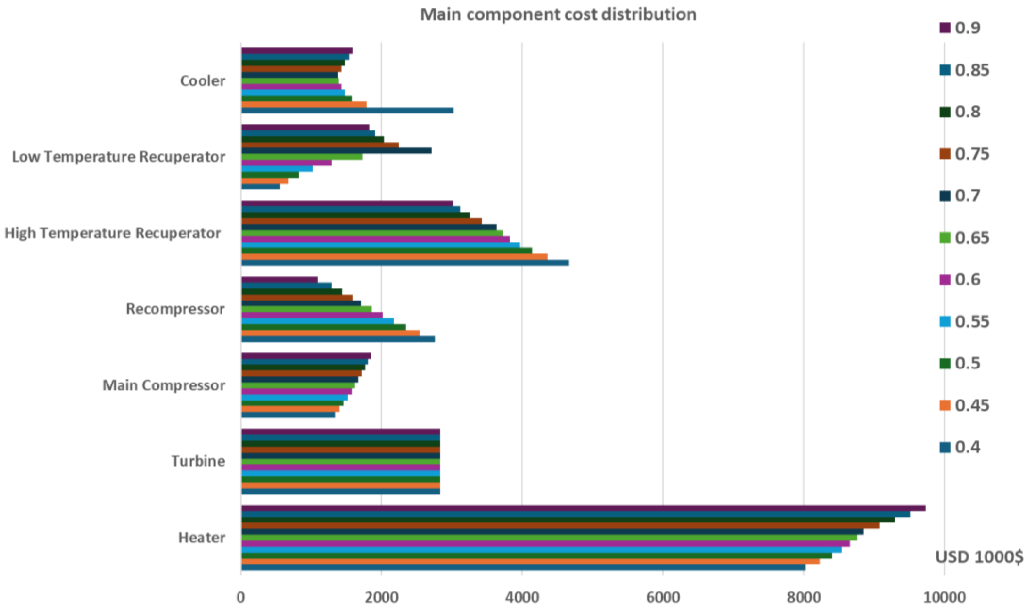
Figure 12.
Recompression cycle thermal efficiency with varying recuperators effectiveness for maximum Heater temperature 973.15K.
Figure 12.
Recompression cycle thermal efficiency with varying recuperators effectiveness for maximum Heater temperature 973.15K.
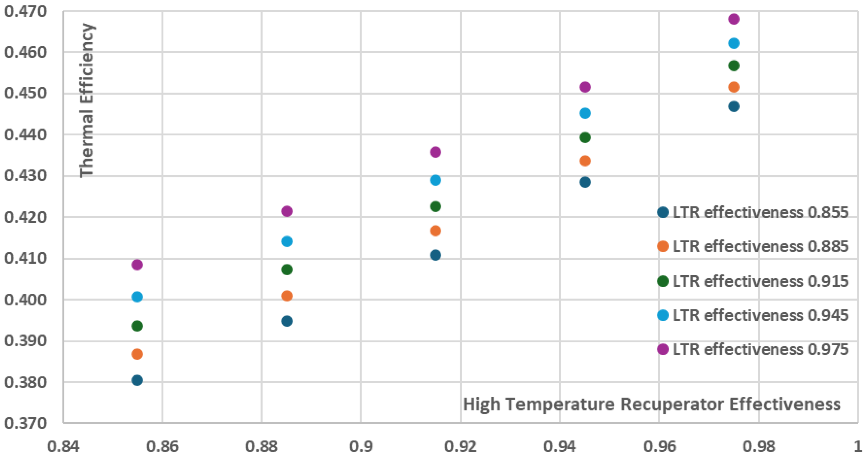
Figure 13.
Recompression cycle net power with varying recuperators effectiveness for maximum Heater temperature 973.15K.
Figure 13.
Recompression cycle net power with varying recuperators effectiveness for maximum Heater temperature 973.15K.
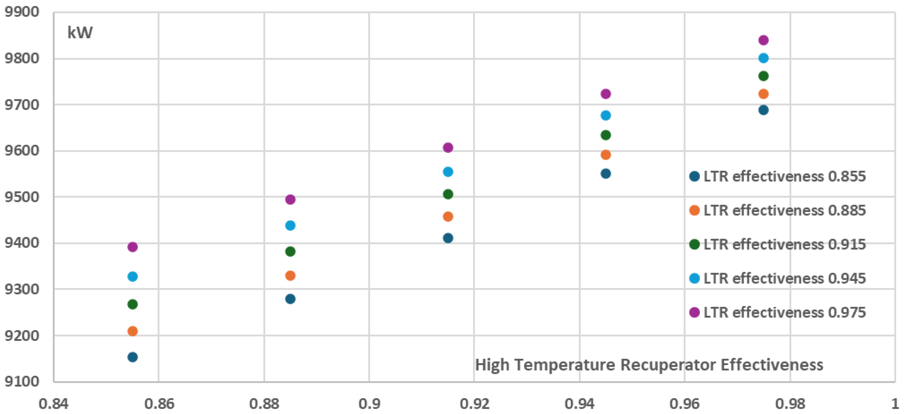
Figure 14.
Recompression cycle cost per net power with varying recuperators effectiveness for maximum Heater temperature 973.15K.
Figure 14.
Recompression cycle cost per net power with varying recuperators effectiveness for maximum Heater temperature 973.15K.
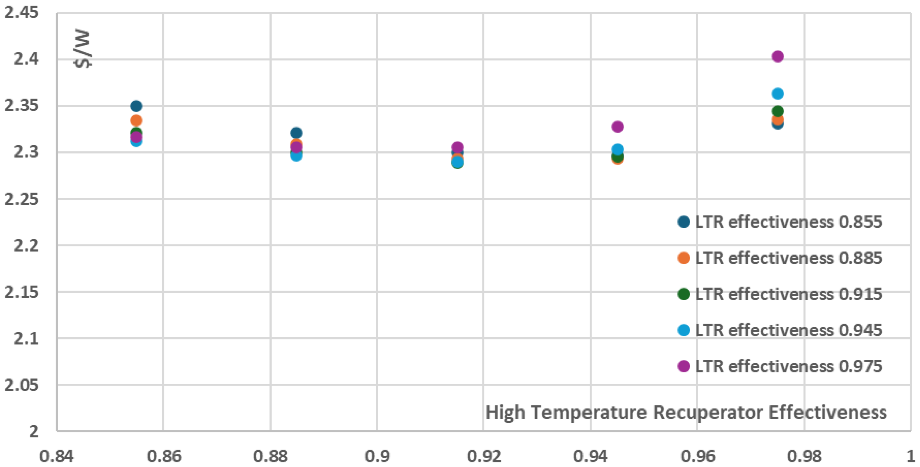
Figure 15.
Recompression cycle thermal efficiency with varying recuperators effectiveness for maximum Heater temperature 823.15K.
Figure 15.
Recompression cycle thermal efficiency with varying recuperators effectiveness for maximum Heater temperature 823.15K.
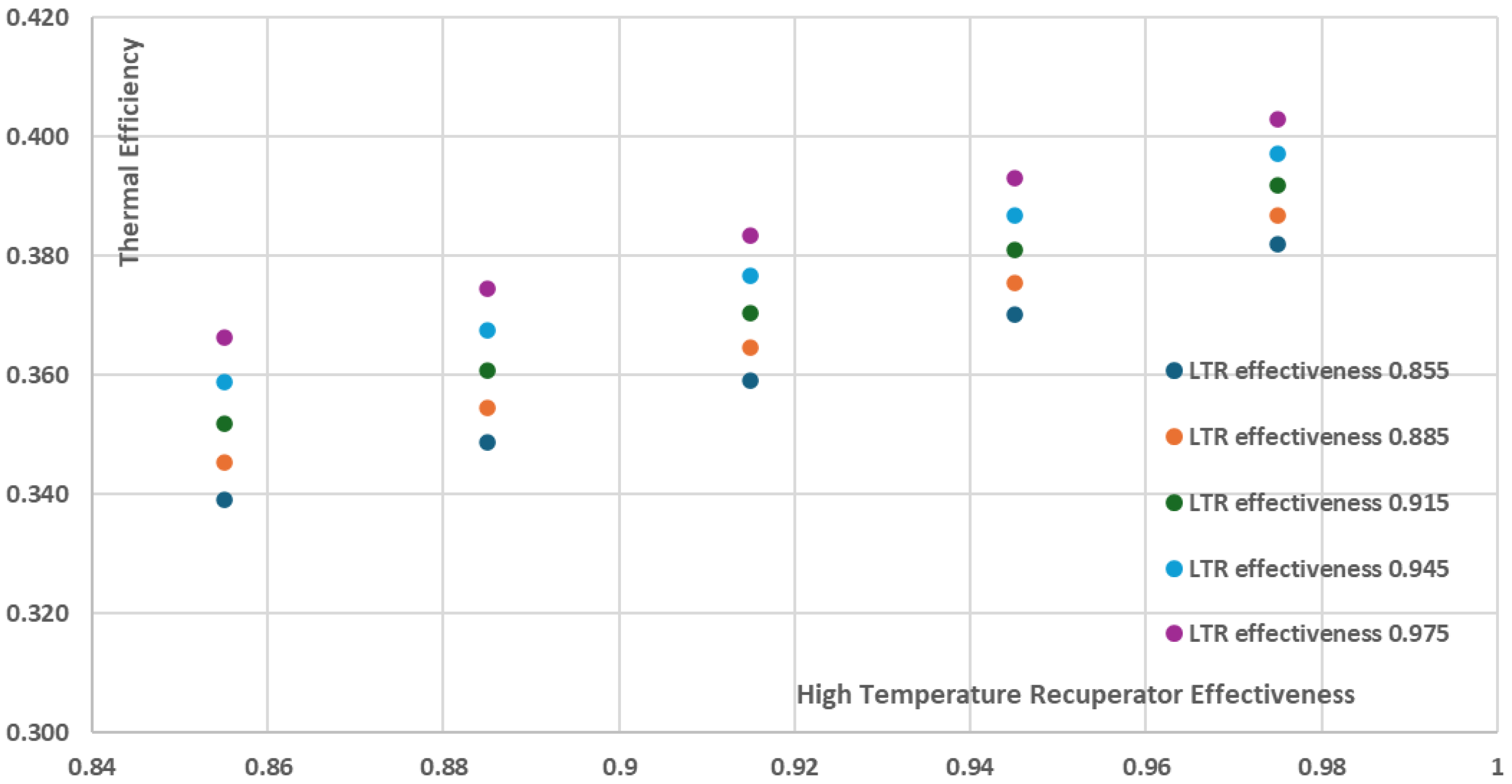
Figure 16.
Recompression cycle net power with varying recuperators effectiveness for maximum Heater temperature 823.15K.
Figure 16.
Recompression cycle net power with varying recuperators effectiveness for maximum Heater temperature 823.15K.
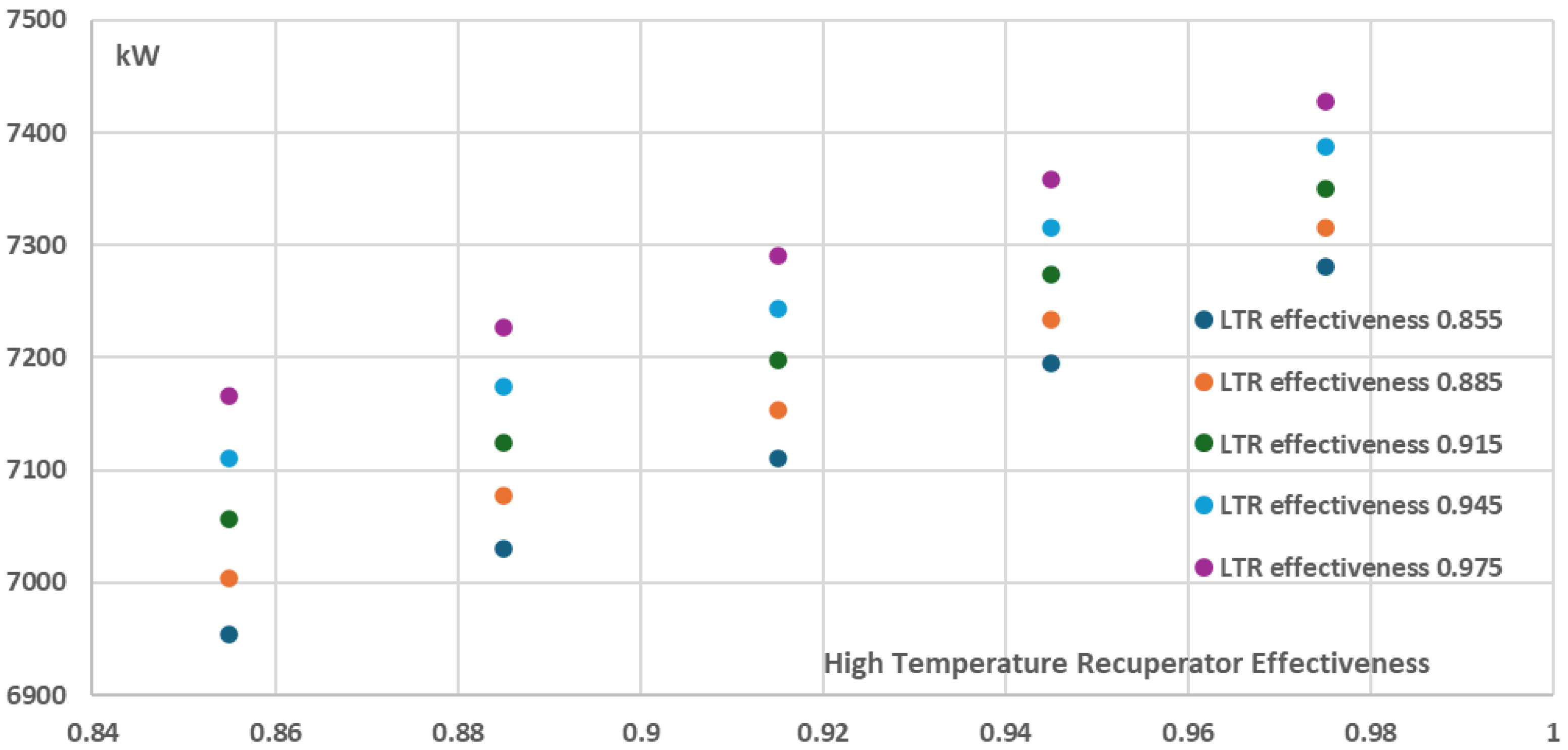
Figure 17.
Recompression cycle cost per net power with varying recuperators effectiveness for maximum Heater temperature 823.15K.
Figure 17.
Recompression cycle cost per net power with varying recuperators effectiveness for maximum Heater temperature 823.15K.
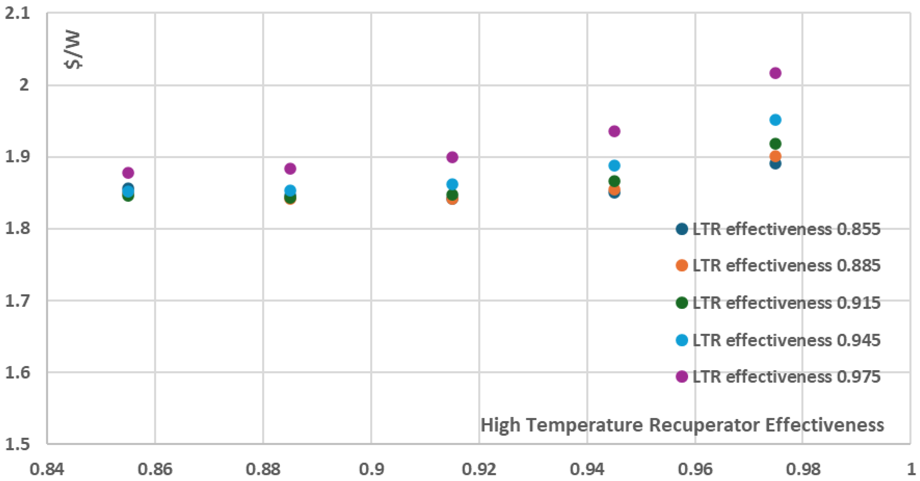
Figure 18.
Recompression cycle thermal efficiency with varying recuperators effectiveness for maximum Heater temperature 873.15K.
Figure 18.
Recompression cycle thermal efficiency with varying recuperators effectiveness for maximum Heater temperature 873.15K.
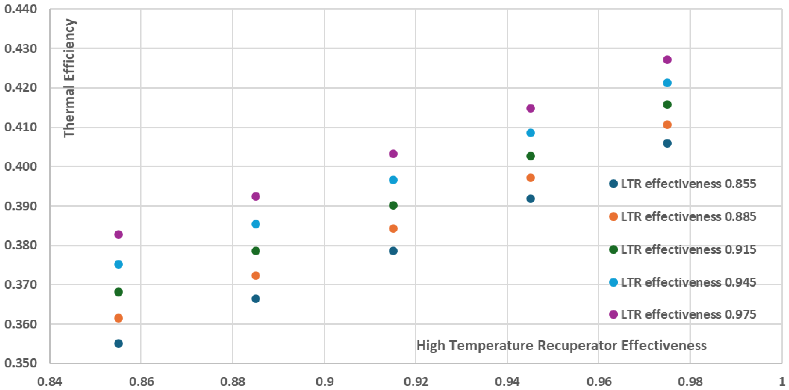
Figure 19.
Recompression cycle net power with varying recuperators effectiveness for maximum Heater temperature 873.15K.
Figure 19.
Recompression cycle net power with varying recuperators effectiveness for maximum Heater temperature 873.15K.
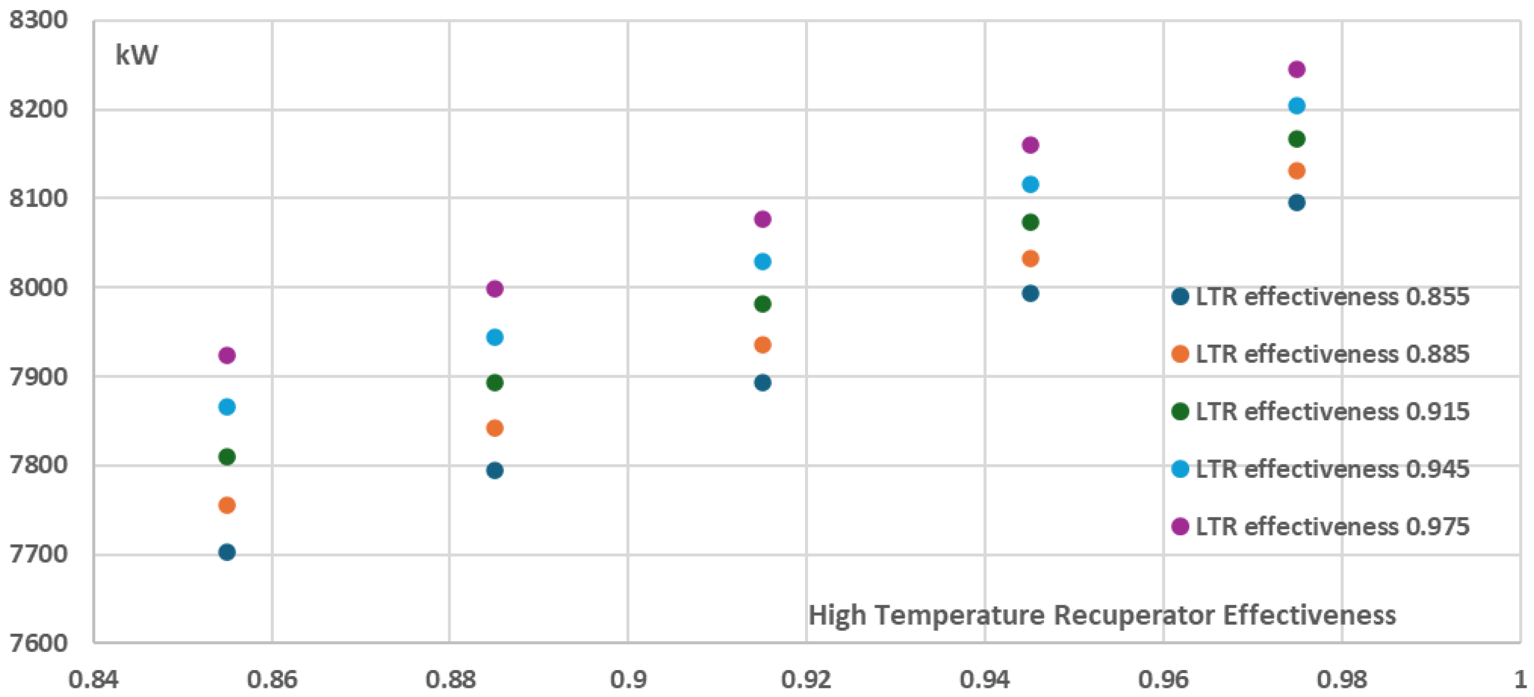
Figure 20.
Recompression cycle cost per net power with varying recuperators effectiveness for maximum Heater temperature 873.15K.
Figure 20.
Recompression cycle cost per net power with varying recuperators effectiveness for maximum Heater temperature 873.15K.
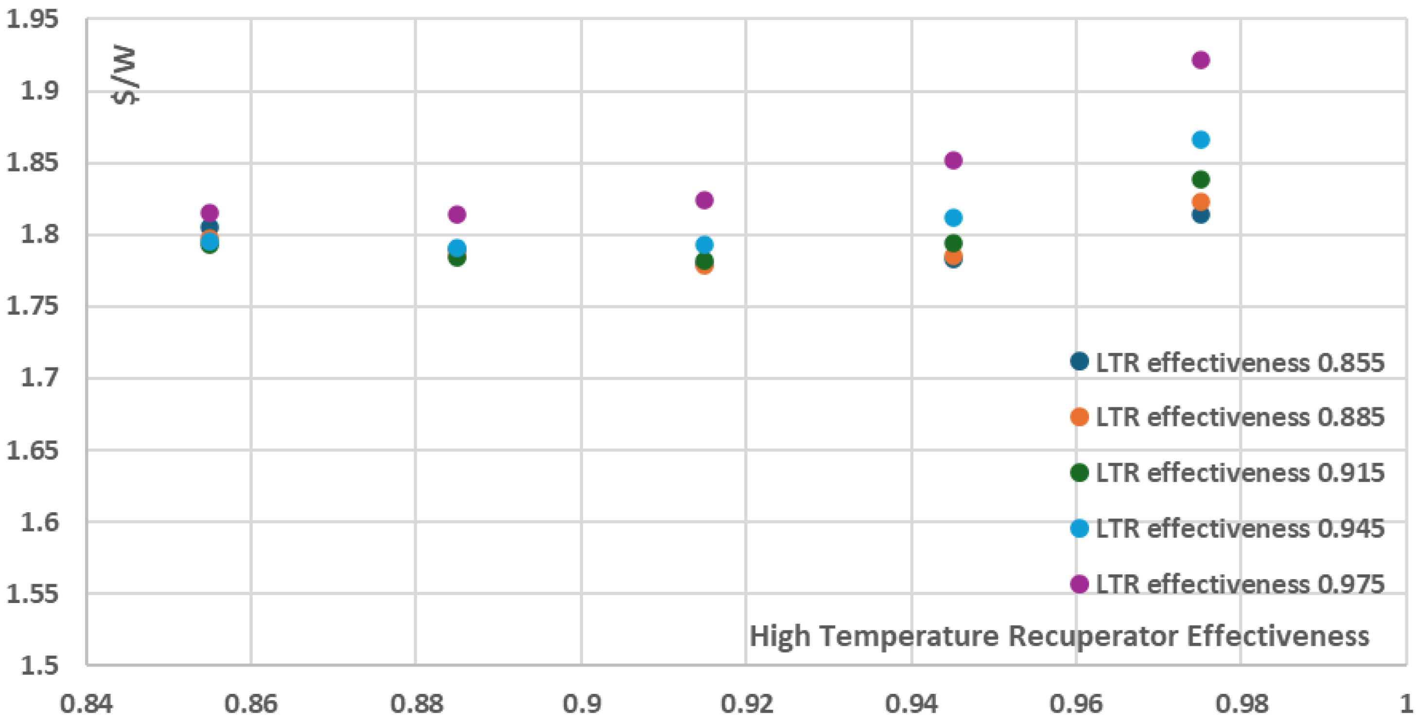
Figure 21.
Recompression cycle thermal efficiency with varying recuperators effectiveness for maximum Heater temperature 923.15K.
Figure 21.
Recompression cycle thermal efficiency with varying recuperators effectiveness for maximum Heater temperature 923.15K.
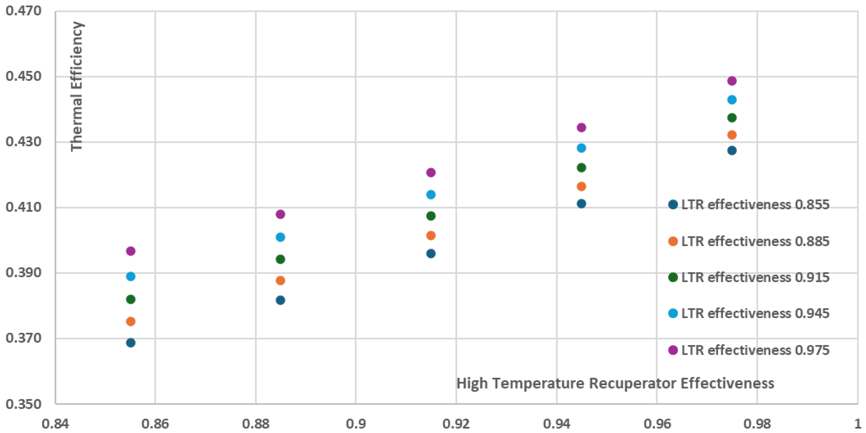
Figure 22.
Recompression cycle net power with varying recuperators effectiveness for maximum Heater temperature 923.15K.
Figure 22.
Recompression cycle net power with varying recuperators effectiveness for maximum Heater temperature 923.15K.
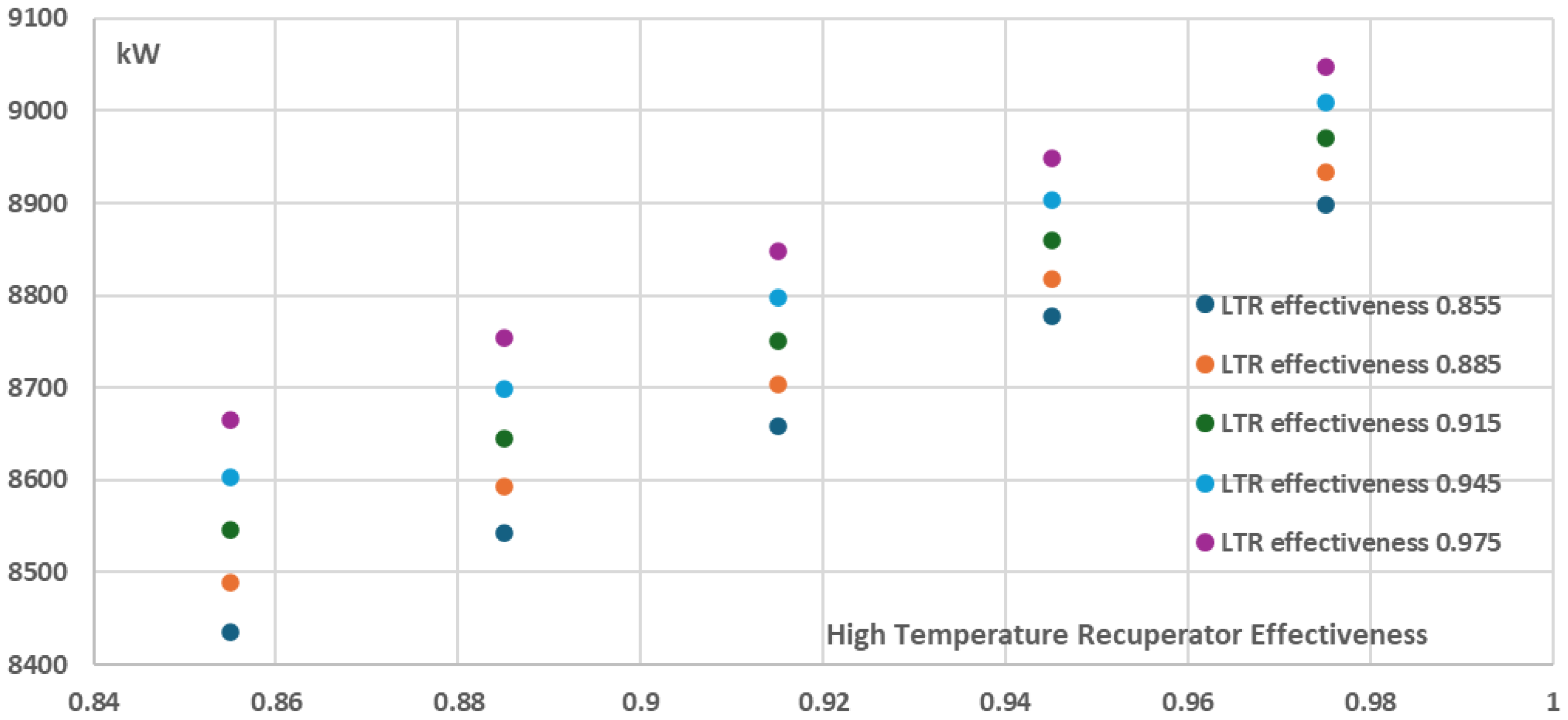
Figure 23.
Recompression cycle cost per net power with varying recuperators effectiveness for maximum Heater temperature 923.15K.
Figure 23.
Recompression cycle cost per net power with varying recuperators effectiveness for maximum Heater temperature 923.15K.
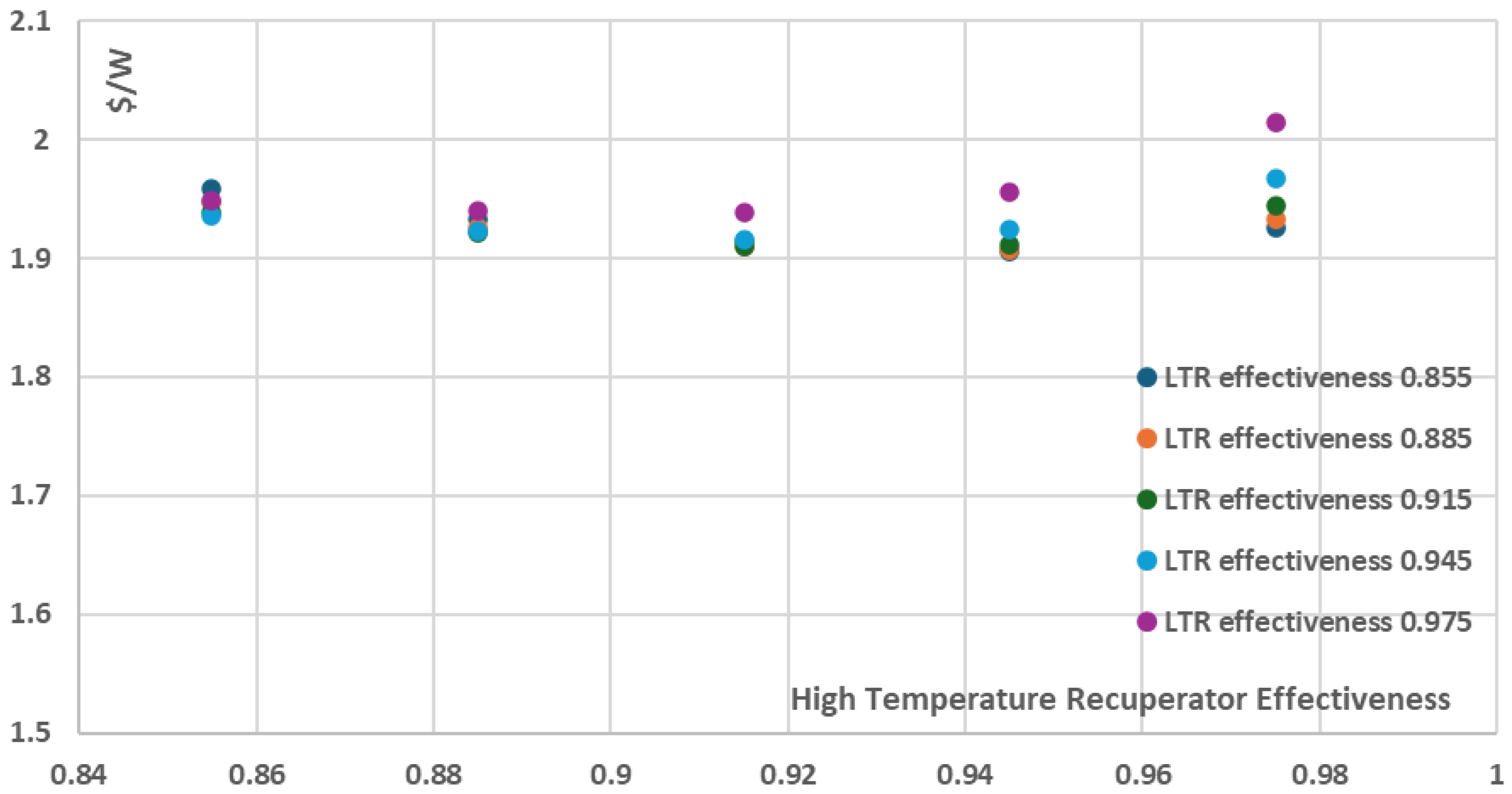
Figure 24.
Recompression cycle thermal efficiency with varying recuperators effectiveness for maximum Heater temperature 1023.15K.
Figure 24.
Recompression cycle thermal efficiency with varying recuperators effectiveness for maximum Heater temperature 1023.15K.
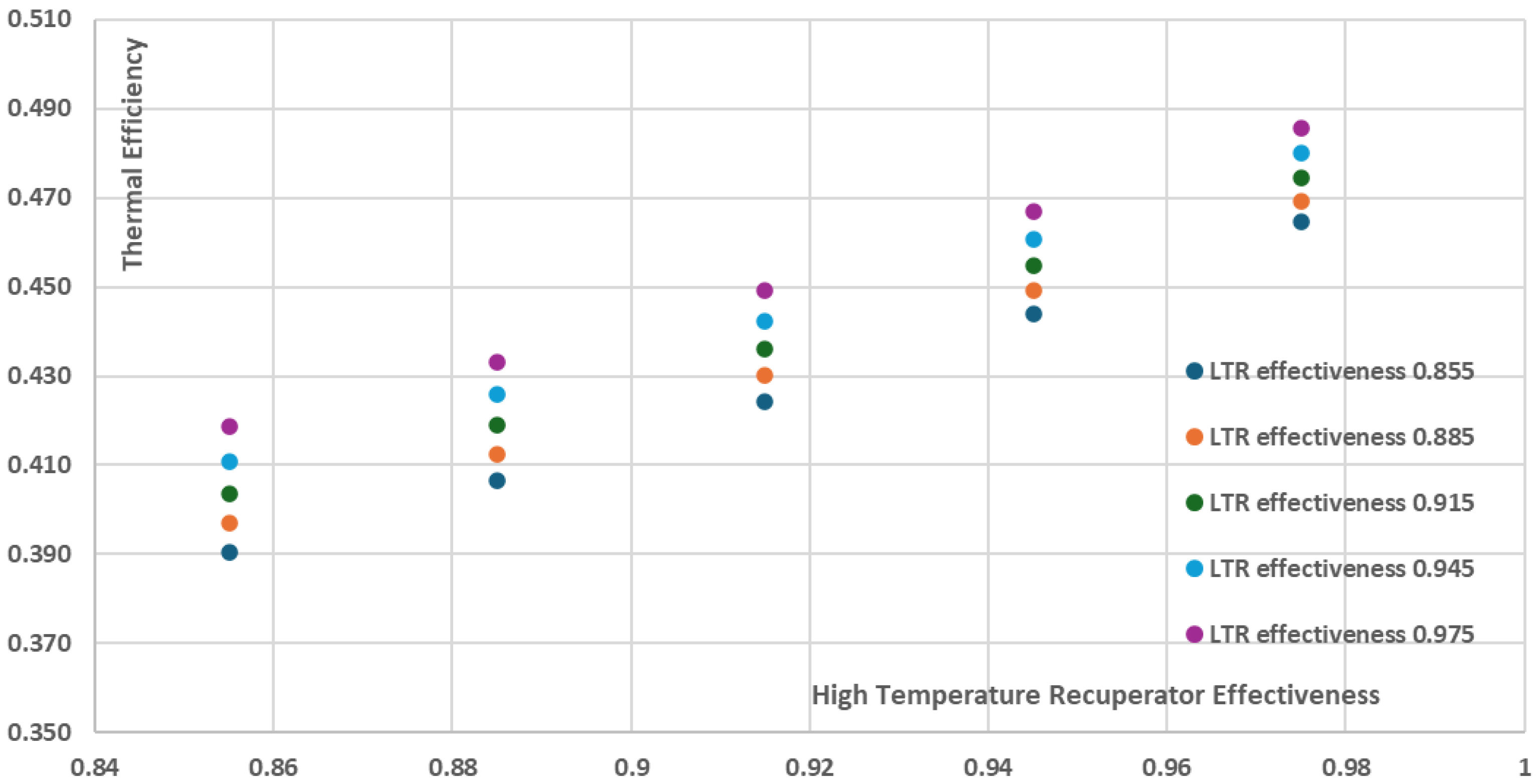
Figure 25.
Recompression cycle net power with varying recuperators effectiveness for maximum Heater temperature 1023.15K.
Figure 25.
Recompression cycle net power with varying recuperators effectiveness for maximum Heater temperature 1023.15K.
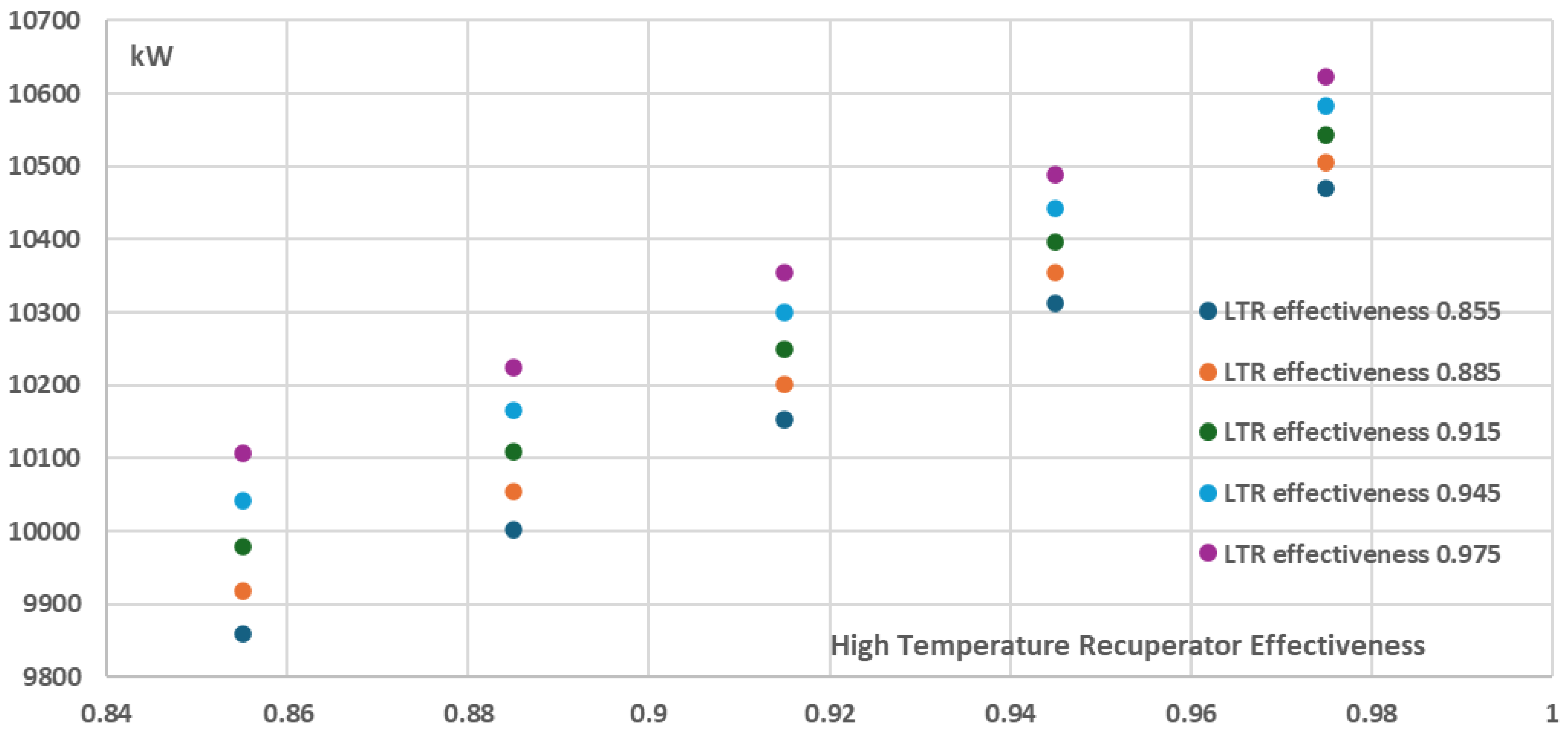
Figure 26.
Recompression cycle cost per net power with varying recuperators effectiveness for maximum Heater temperature 1023.15K.
Figure 26.
Recompression cycle cost per net power with varying recuperators effectiveness for maximum Heater temperature 1023.15K.
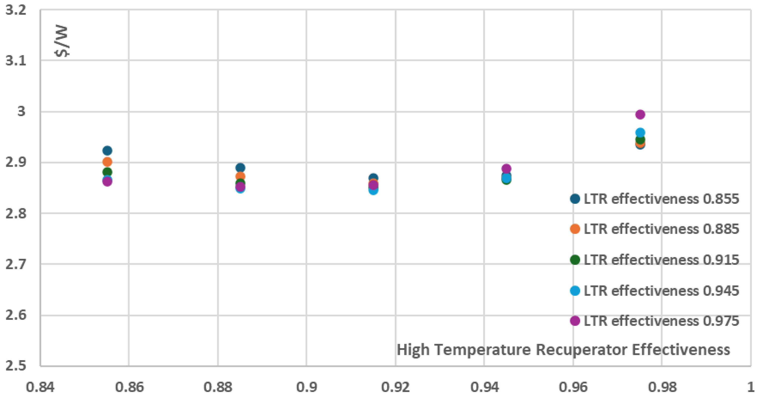
Figure 15.
Cost Correction Function in relation to Heater maximum temperature.
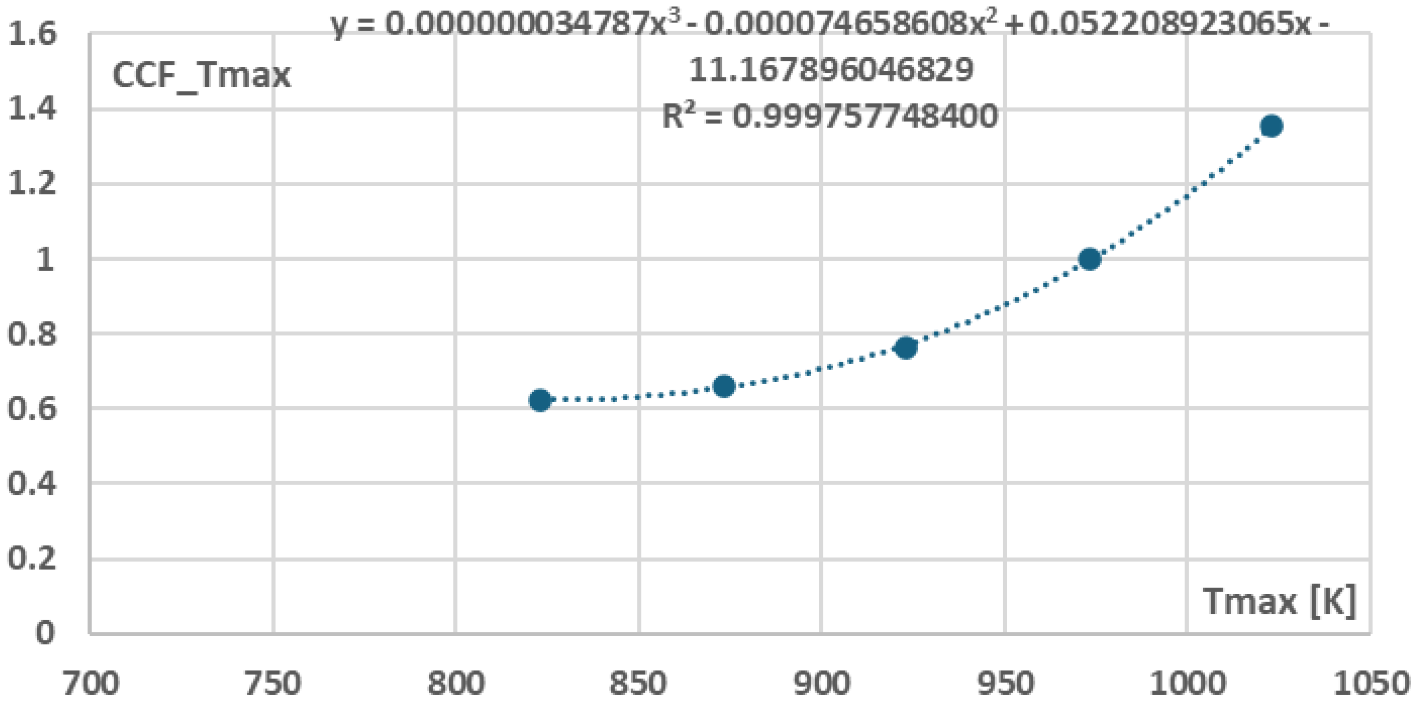
Figure 27.
Cost Correction Function in relation to High Temperature Recuperator effectiveness for Low Temperature Recuperator effectiveness equal to 0.855.
Figure 27.
Cost Correction Function in relation to High Temperature Recuperator effectiveness for Low Temperature Recuperator effectiveness equal to 0.855.
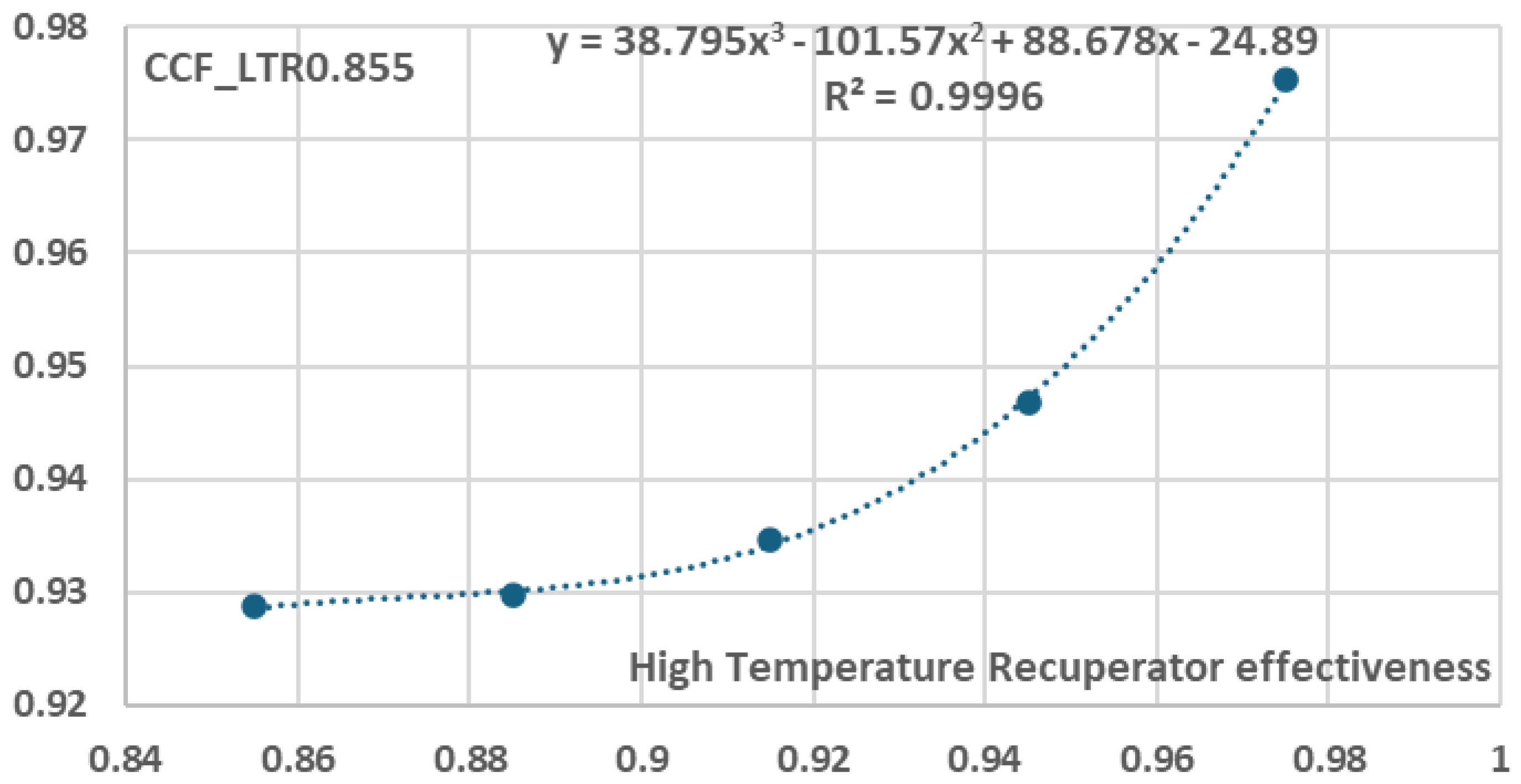
Figure 28.
Cost Correction Function in relation to High Temperature Recuperator effectiveness for Low Temperature Recuperator effectiveness equal to 0.885.
Figure 28.
Cost Correction Function in relation to High Temperature Recuperator effectiveness for Low Temperature Recuperator effectiveness equal to 0.885.
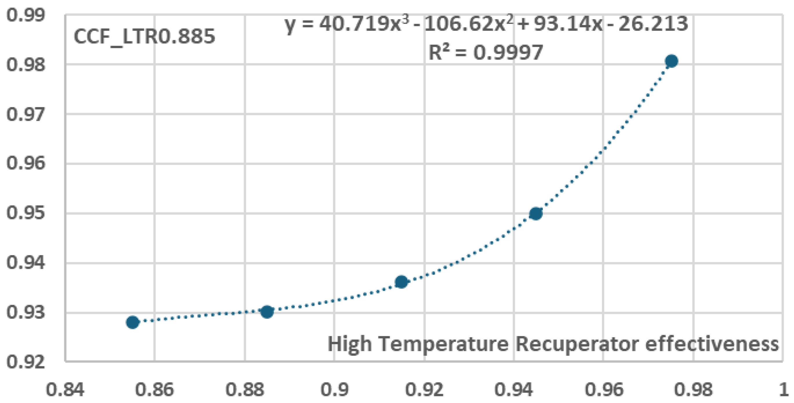
Figure 29.
Cost Correction Function in relation to High Temperature Recuperator effectiveness for Low Temperature Recuperator effectiveness equal to 0.915.
Figure 29.
Cost Correction Function in relation to High Temperature Recuperator effectiveness for Low Temperature Recuperator effectiveness equal to 0.915.
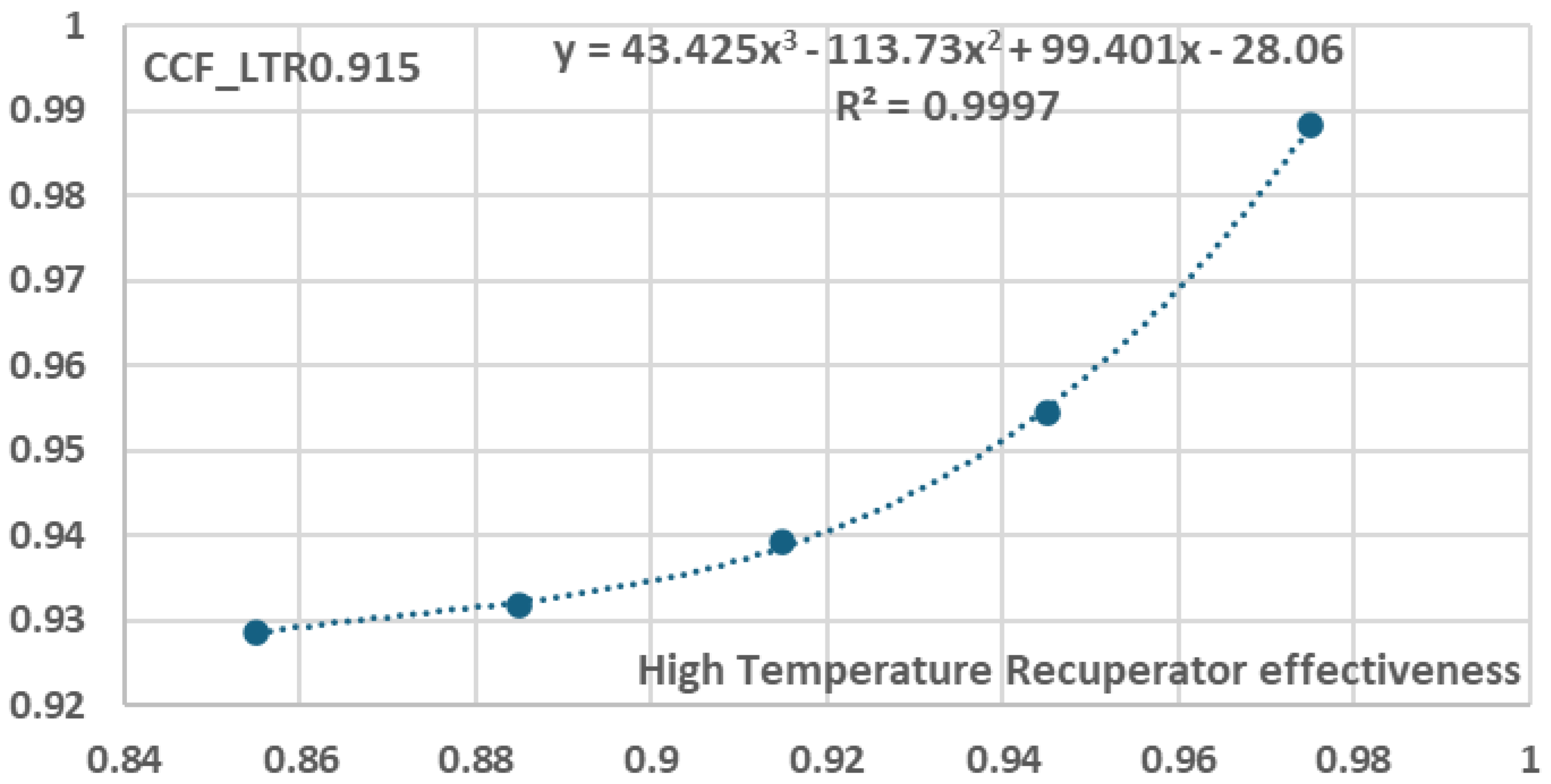
Figure 30.
Cost Correction Function in relation to High Temperature Recuperator effectiveness for Low Temperature Recuperator effectiveness equal to 0.945.
Figure 30.
Cost Correction Function in relation to High Temperature Recuperator effectiveness for Low Temperature Recuperator effectiveness equal to 0.945.
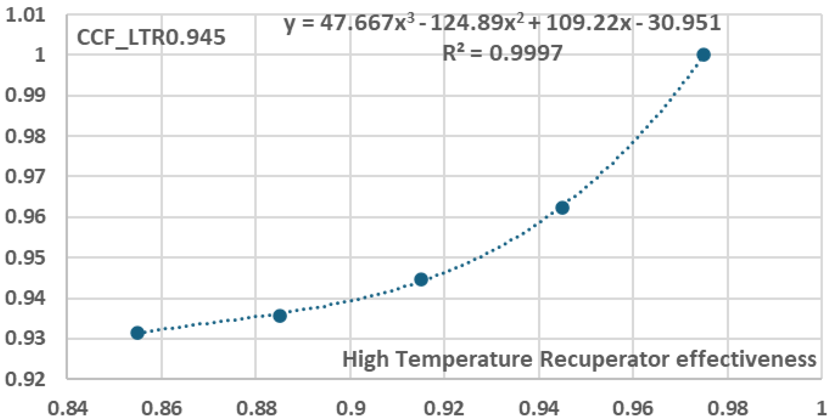
Figure 31.
Cost Correction Function in relation to High Temperature Recuperator effectiveness for Low Temperature Recuperator effectiveness equal to 0.975.
Figure 31.
Cost Correction Function in relation to High Temperature Recuperator effectiveness for Low Temperature Recuperator effectiveness equal to 0.975.
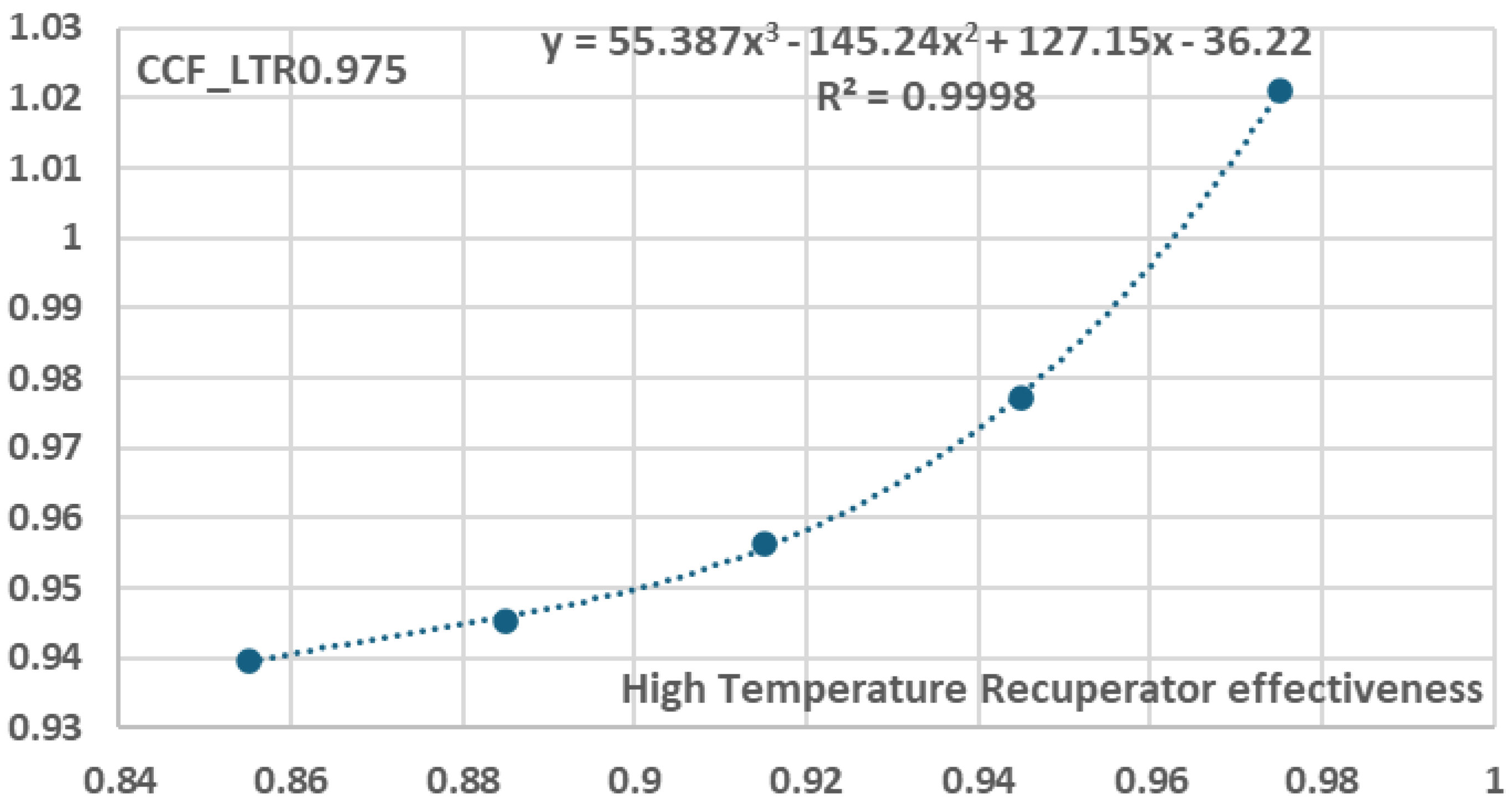
Figure 32.
Variation of coefficient in relation to Low Temperature Recuperator effectiveness.
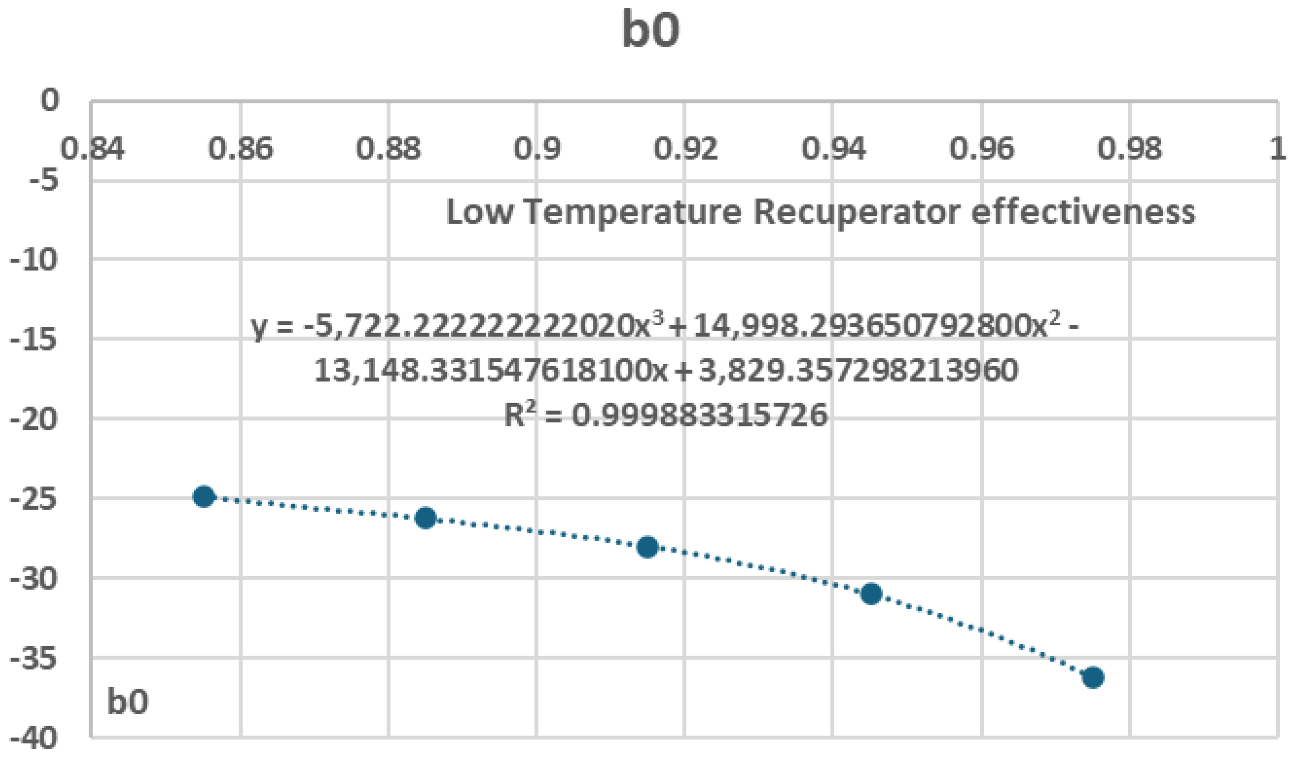
Figure 33.
Variation of coefficient in relation to Low Temperature Recuperator effectiveness.
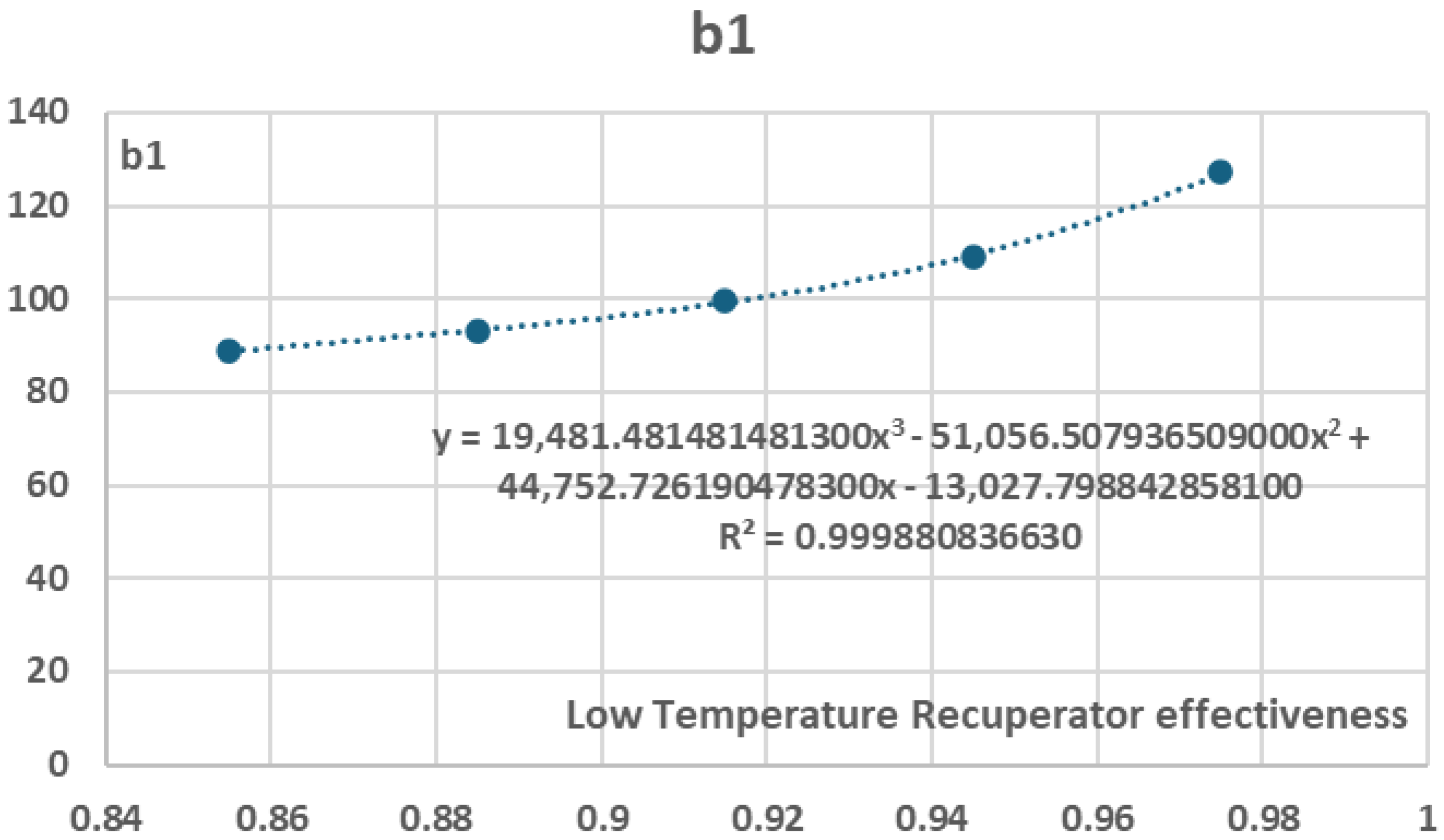
Figure 34.
Variation of coefficient in relation to Low Temperature Recuperator effectiveness.
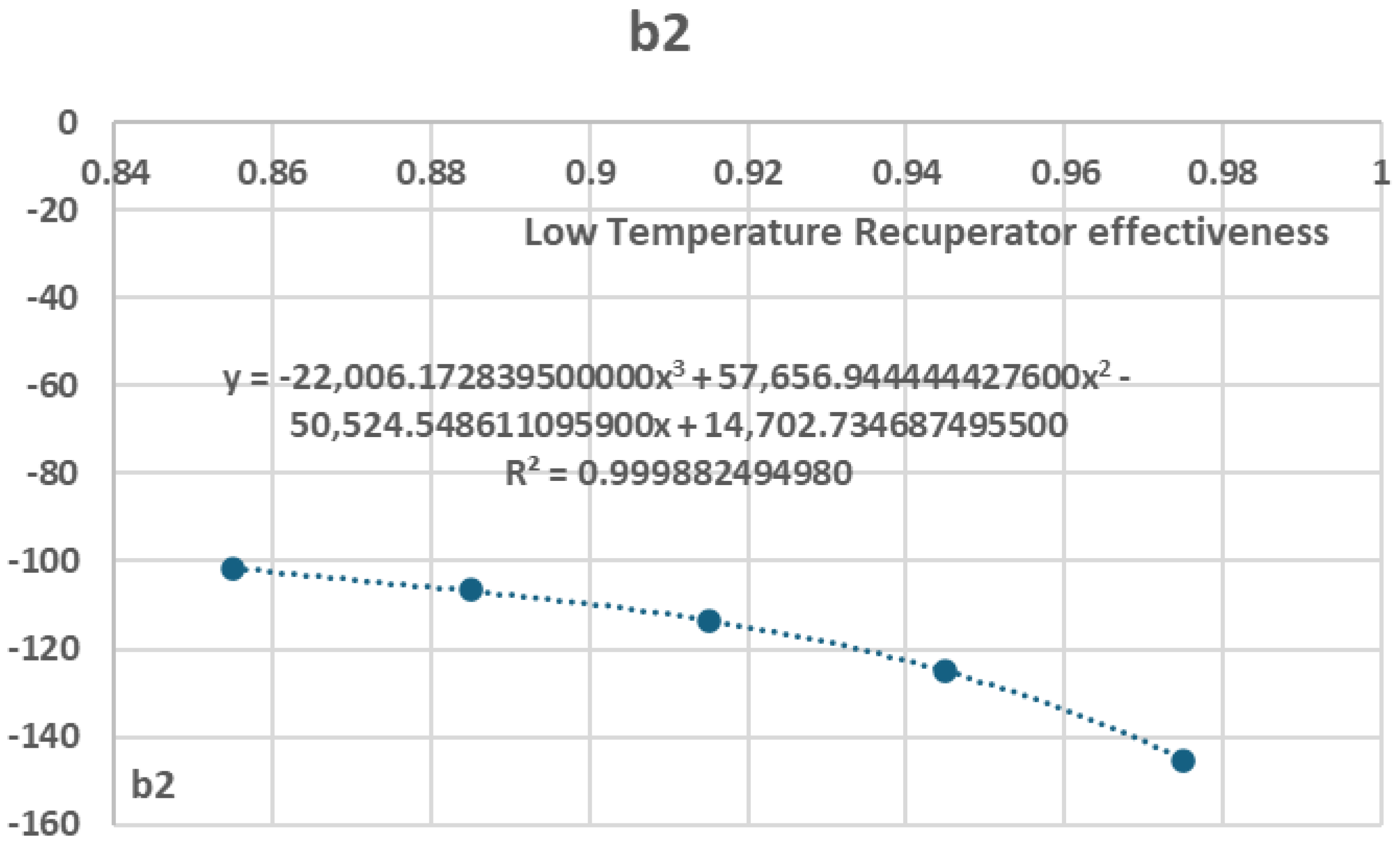
Figure 35.
Variation of coefficient in relation to Low Temperature Recuperator effectiveness.
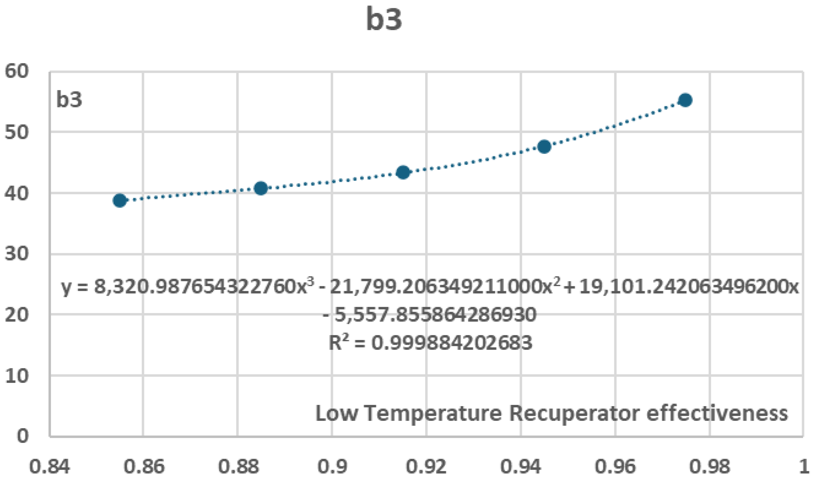
Figure 36.
Difference % of results from cost function with data from parametric analysis.
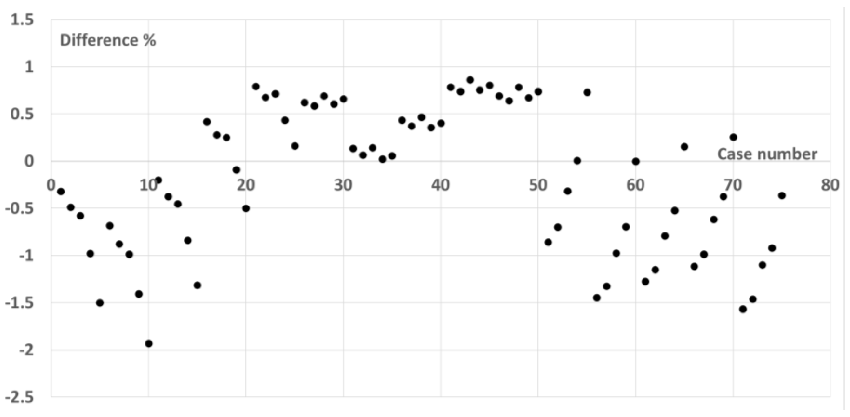

Table 1.
Main advantages of s-CO2 as working fluid and s-CO2 Brayton cycle.
| s-CO2 as working fluid advantages | s-CO2 Brayton cycle advantages |
|---|---|
| • Environmentally friendly, pollution free and abundant fluid, widely available, low-cost, low toxicity, low corrosivity | o Favourable conditions for recuperation and internal heat exchange due to convenient s-CO2 properties, resulting to highly effective recuperators which for the case of recompression cycle layouts can reduce the cooling demands |
| • High density working fluid resulting to the use of highly compact turbomachinery and heat exchangers | o Increased cycle adaptability by the integration of other possible heat exchange processes (e.g. intercooling, recuperation, reheating) providing design adaptability to operational conditions and power demand |
| • Single phase working fluid resulting to reduced operational complexity and simpler cycle design than steam Rankine cycles | o Competitive performance with dry air cooling, especially for more sophisticated component technology level, resulting to lower operational and capital costs. |
| • Thermally stable at high temperatures of interest to high temperature applications, e.g. for CSP, from 550 °C to 750 °C | o Used in power cycles with higher efficiency (s-CO2 Brayton cycles) |
| • s-CO2 integrates well with sensible heat storage units in solar systems | |
| • s-CO2 has convenientheat transfer properties (density, viscosity, thermal conductivity, heat capacity) | |
| • s-CO2 critical temperature similar to ambient conditions | |
Table 2.
Supercritical carbon dioxide Brayton cycle main components description.
| ➢ Primary Heater (Heater): in the primary heater the already preheated (in the High Temperature Recuperator) supercritical carbon dioxide absorbs heat from an external heat source (e.g. natural gas, solar energy, waste heat) and achieves its maximum temperature (~1000K) getting ready for expansion. The heat addition process is not isobaric as pressure losses are presented in the working fluid. |
|---|
| ➢ Turbine (Turbine_CO2): The supercritical carbon dioxide expands in the Turbine converting heat to mechanical work. Due to the high density of the supercritical state the turbine can be significantly smaller than the one for conventional Brayton cycles of similar temperature level conditions. The Turbine expansion results in sCO2 pressure and temperature decrease and at the Turbine outlet the partially expanded supercritical working fluid is still at a relatively high temperature level. |
| ➢ High Temperature Recuperator (High_Temperature_HEX): The High Temperature Recuperator is a heat exchanger (typically of counter-flow or cross-counterflow arrangement) where heat is extracted from the sCO2 Turbine outlet and, instead of being rejected as waste heat, it is transferred its back into the recompression cycle. This recuperation process results in the preheating of the working fluid before the heat addition in the Primary Heater and thus, improves the cycle efficiency. In the recuperation process the effectiveness and pressure losses are critical parameters in the maximization of thermal energy recovery and the increase of cycle efficiency. |
| ➢ Low Temperature Recuperator (Low_Temperature_HEX): The Low Temperature Heat Exchanger is a heat exchanger (typically of counter-flow or cross-counterflow arrangement) where the supercritical carbon dioxide, cooled initially at the High Temperature Recuperator, preheats the compressed fluid coming out from the Main Compressor. This additional recuperation process reduces the wasted thermal energy to the environment and improves cycle efficiency. Furthermore, the working fluid temperature increases before it enters the Recompressor as it recovers heat from Turbine exhaust. |
| ➢ Flow Splitter (Splitter): After the Low Temperature Recuperator, the working fluid stream is divided into two paths, i.e. the primary flow and the bypass flow. The primary flow passes through the Cooler and the Main Compressor while the bypass flow passes through the Recompressor, thus, bypassing the Cooler, reducing the heat losses and enhancing cycle efficiency. The flow split ratio is defined as the ratio of the Main Compressor mass flow rate to the total flow mass flow rate. |
| ➢ Cooler (Cooler): The working fluid after passing though the High and Low Temperature Recuperators is still at moderate temperature. In order to be cooled down, the working fluid passes through a heat exchanger (Cooler) where heat is being extracted by another cooling medium (usually air or water). |
| ➢ Main Compressor (Main_Compressor): After the Cooler the working fluid passes through the Main Compressor in supercritical state, having high density and low temperature values, requiring less work in relation to comparable Brayton cycle compression process. |
| ➢ Recompressor or Bypass Compressor (Recompressor): The Recompressor is fed with the bypass stream of the working fluid coming out of the Flow Splitter and the working fluid is compressed. This compression process is performed at a higher mean temperature since the bypass stream of the working fluid has not been cooled down in the Cooler. |
| ➢ Flow Mixer (Mixer): The Mixer merges the two streams, the recompressed stream and the Main Compressor stream as the latter has passed through the Low Temperature Recuperator so that the combined, mixed, stream enters the High Temperature Recuperator. |
Table 3.
Developed components main inlet parameters and outlet results.
| Component | Known conditions/properties | Calculations and Outlet results |
|---|---|---|
| Heater | Outlet Temperature, Pressure loss coefficient | Heat Duty, Pressure losses |
| Turbine_CO2 | Outlet pressure, Isentropic efficiency |
Turbine work, Turbine power |
| High_Temperature_HEX | Thermal effectiveness, Hot/cold flows pressure loss coefficients |
Heat exchange, Pressure losses, UA (conductance-area product) |
| Low_Temperature_HEX | Thermal effectiveness, Hot/cold flows pressure loss coefficients |
Heat exchange, Pressure losses, UA (conductance-area product) |
| Splitter | Split ratio, Pressure drop | Main stream mass flow rate, Bypass stream mass flow rate |
| Cooler | Outlet Temperature, Pressure loss coefficient, Cooling fluid (air) specific heat, Cooling fluid (air) inlet temperature, Cooling fluid (air) temperature difference increase ratio in relation to CO2 temperature decrease |
Heat Duty, Pressure losses, UA (conductance-area product), Cooling fluid temperature increase, cooling fluid required mass flow rate |
| Main_Compressor | Pressure ratio, Isentropic efficiency | Main Compressor work, Main Compressor power |
| Recompressor | Pressure ratio, Isentropic efficiency | Recompressor work, Recompressor power |
| Mixer | Main stream mass flow rate, Bypass stream mass flow rate, Pressure-drop |
Total mass flow rate |
Table 4.
Recompression cycle components cost models, Weiland et al., [9].
Table 4.
Recompression cycle components cost models, Weiland et al., [9].
| Component | α | B | C | d | Scale parameter |
|---|---|---|---|---|---|
| Heater | 632900 | 0.6 | 0 | 0.000054 | Power [MW] |
| Turbine | 182600 | 0.5561 | 0 | 0.000106 | Power [MW] |
| Dry Cooler | 32.88 | 0.75 | 0 | 0 | UA [W/K] |
| Low Temperature Recuperator | 49.45 | 0.7554 | 0.02131 | 0 | UA [W/K] |
| High Temperature Recuperator | 49.45 | 0.7554 | 0.02131 | 0 | UA [W/K] |
| Main Compressor | 1230000 | 0.3992 | 0 | 0 | Power [MW] |
| Recompressor | 1230000 | 0.3992 | 0 | 0 | Power [MW] |
| Motor | 131400 | 0.5611 | 0 | 0 | Power [MW] |
| Generator | 108900 | 0.5463 | 0 | 0 | Power [MW] |
| Gearbox | 177200 | 0.2434 | 0 | 0 | Power [MW] |
| Component | Validation Case 1: Weiland et al. | Validation Case 2: Drennen and Lance |
|---|---|---|
| Heater | Tmax=973.15K DP=6bar |
Tmax=823.15K DP/P=0.8% |
| Turbine | nt=85% Outlet pressure=90bar |
nt=85% Outlet pressure=76.8bar |
| Cooler | Tcooler=306.6K DP=1.8bar |
Tcooler=305K DP/P=0.8% |
| Low Temperature Recuperator | nreg=0.945 DP=1.8bar |
nreg=0.95 DP/P=0.8% |
| High Temperature Recuperator | nreg=0.975 DP=1.8bar |
nreg=0.95 DP/P=0.8% |
| Main Compressor | nc=82% Pressure ratio=2.96 |
nc=82% Pressure ratio= 4.67 |
| Recompressor | nc=78% Pressure ratio=2.87 |
nc=78% Pressure ratio= 4.59 |
| Splitter | Split ratio=0.65 | Split ratio=0.70 |
| Mass flow rate | 99.5kg/s | 210.1kg/s |
Table 6.
Comparison between COCO model and Validation Case1 (Weiland et al., [9]).
Table 6.
Comparison between COCO model and Validation Case1 (Weiland et al., [9]).
| Net Power ~10MW | COCO_model | Validation Case 1 | Unit | Relative difference % |
|---|---|---|---|---|
| Heater | 21.20 | 21.81 | MW | -2.80 |
| Turbine | 14.62 | 14.62 | MW | 0.01 |
| HEX_HT_REC | 43.91 | 44.87 | MW | -2.13 |
| HEX_LT_REC | 14.57 | 14.60 | MW | -0.22 |
| Main_Compressor | 2.00 | 1.81 | MW | 10.71 |
| Recompressor | 2.82 | 2.59 | MW | 8.77 |
| Cooler | 11.40 | 11.59 | MW | -1.65 |
| UA_HEX_HT_REC | 1555.48 | not available | kW/K | - |
| UA_HEX_LT_REC | 1058.42 | not available | kW/K | - |
| Net Power | 9.80 | 10.22 | MW | -4.11 |
| Thermal efficiency | 46.23 | 46.86 | % | -1.34 |
Table 7.
Comparison between COCO model and Validation Case2 Drennen and Lance [8]).
Table 7.
Comparison between COCO model and Validation Case2 Drennen and Lance [8]).
| Net Power ~20MW | COCO_model | Validation Case 2 | Unit | Relative difference % |
|---|---|---|---|---|
| Heater | 49.89 | 49.70 | MW | 0.37 |
| Turbine | 38.72 | 38.40 | MW | 0.84 |
| High Temperature Recuperator | 17.15 | 17.20 | MW | -0.28 |
| Low Temperature Recuperator | 43.67 | 43.30 | MW | 0.86 |
| Main_Compressor | 9.58 | 9.00 | MW | 6.45 |
| Recompressor | 10.11 | 9.50 | MW | 6.47 |
| Cooler | 30.86 | 29.70 | MW | 3.90 |
| UA_HEX_HT_REC | 2184.45 | 2230.00 | kW/K | -2.04 |
| UA_HEX_LT_REC | 6840.86 | 6970.00 | kW/K | -1.85 |
| Net Power | 19.03 | 19.90 | MW | -4.39 |
| Thermal efficiency | 38.14 | 40.04 | % | -4.74 |
Table 8.
Comparison between COCO model and Validation Case1 (Weiland et al., [9]).
Table 8.
Comparison between COCO model and Validation Case1 (Weiland et al., [9]).
| COCO Model | Weiland et al. | |||
|---|---|---|---|---|
| Component | Net Cost k$ | Cost % | Net Cost k$ | Cost % |
| Heater | 8760 | 37.82 | 8909 | 38.22 |
| Turbine | 2831 | 12.22 | 2831 | 12.14 |
| High Temperature Recuperator | 3721 | 16.03 | 3324 | 14.26 |
| Low Temperature Recuperator | 1726 | 7.49 | 2056 | 8.82 |
| Main_Compressor | 1623 | 7.01 | 1558 | 6.68 |
| Recompressor | 1860 | 8.03 | 1798 | 7.71 |
| Dry Cooler (with Fan) | 1397 | 6.03 | 1617 | 6.94 |
| Motors | 429 | 1.85 | 407 | 1.75 |
| Generator | 471 | 2.04 | 471 | 2.02 |
| Gearbox | 340 | 1.47 | 340 | 1.46 |
| Total | $23160 | 100.00% | $23311 | 100.00% |
Table 9.
Minimum cost per net power in relation to maximum temperature and recuperators effectiveness.
Table 9.
Minimum cost per net power in relation to maximum temperature and recuperators effectiveness.
| Tmax | Minimum cost per net power $/W | LTR effectiveness | HTR effectiveness |
|---|---|---|---|
| 823.15K | ~1.85 | From 0.885 to 0.915 | From 0.885 to 0.915 |
| 873.15K | ~1.78 | From 0.885 to 0.915 | From 0.885 to 0.915 |
| 923.15K | ~1.91 | From 0.885 to 0.915 | From 0.915 to 0.945 |
| 973.15K | ~2.29 | 0.915 | 0.915 |
| 1023.15K | ~2.85 | 0.945 | From 0.885 to 0.915 |
Table 10.
Variation of b coefficients in relation to Low Temperature Recuperator effectiveness.
| 0.855 | -24.89 | 88.678 | -101.57 | 38.795 |
| 0.885 | -26.213 | 93.14 | -106.62 | 40.719 |
| 0.915 | -28.06 | 99.401 | -113.73 | 43.425 |
| 0.945 | -30.951 | 109.22 | -124.89 | 47.667 |
| 0.975 | -36.22 | 127.15 | -145.24 | 55.387 |
Disclaimer/Publisher’s Note: The statements, opinions and data contained in all publications are solely those of the individual author(s) and contributor(s) and not of MDPI and/or the editor(s). MDPI and/or the editor(s) disclaim responsibility for any injury to people or property resulting from any ideas, methods, instructions or products referred to in the content. |
© 2025 by the authors. Licensee MDPI, Basel, Switzerland. This article is an open access article distributed under the terms and conditions of the Creative Commons Attribution (CC BY) license (http://creativecommons.org/licenses/by/4.0/).
Copyright: This open access article is published under a Creative Commons CC BY 4.0 license, which permit the free download, distribution, and reuse, provided that the author and preprint are cited in any reuse.


