
Submitted:
29 January 2025
Posted:
29 January 2025
You are already at the latest version
Abstract
To investigate the aerodynamic characteristics and multi-objective optimization of the variable camber transonic airfoils, the influence of leading and trailing edge deflection angles on aerodynamic performance is analyzed under different angles of attack and Mach numbers. A prediction model is developed based on a Kriging surrogate model, with leading and trailing edge deflection angles as inputs and lift coefficients and drag coefficients as outputs, NSGA-II multi-objective optimization algorithm is employed to determine the optimal deflection parameters for Mach numbers of 0.74, 0.75, and 0.76. The results show that leading edge upward deflection contributes to improve the lift-to-drag ratio, while downward deflection enhances the critical angle of attack. The trailing edge deflection has a relatively minor effect on the critical angle of attack, the downward deflection can improve the lift coefficient. Additionally, appropriate upward deflections of both the leading and trailing edges can delay the critical Mach number, while downward deflections of both edges can advance the critical Mach number. Compared to the basic airfoil, the optimized airfoil reduces the drag coefficient by 22.92%, 43.88% and 56.31% at the three Mach numbers, and increases the lift-to-drag ratio by 11.13%, 20.65%, and 24.89%, respectively, resulting in significant aerodynamic performance enhancement. The prediction errors between the Kriging model and simulation values are less than 6%, effectively improving computational efficiency.
Keywords:
Transonic Airfoil
; Kriging Surrogate Model
; Variable Camber
; Leading and Trailing Edges
; Multi-objective Optimization
1. Introduction
According to flight conditions and mission requirements, the variable camber wing can smoothly and continuously deform its leading and trailing edges, maintain optimal aerodynamic performance and expand its flight envelope [1], with its low energy consumption and high cruising efficiency, the variable camber wing has become a hot spot in the field of morphing aircraft design. In recent years, some companies such as Boeing, NASA, and Airbus have successively launched projects on Variable Camber Flexible Wings (VCFW) [0], the feasibility of smooth and continuous variable camber wings has been demonstrated through the use of smart materials and flexible structures.
The variable camber of the leading and trailing edges can transform the base airfoil into a laminar flow airfoil, which can enhance lift and reduce drag by increasing the airfoil camber. Currently, many researchers have conducted extensive studies focusing on the aerodynamic performance analysis and structural design of variable camber wings. Kaul et al. investigated the aerodynamic effects of trailing-edge camber in the Variable Camber Continuous Trailing Edge Flap (VCCTEF) project [3], the results demonstrated that appropriate trailing-edge deflection improves the lift-to-drag ratio [4,5], however, excessive downward deflection angles increase drag. The computed lift increments showed good agreement with theoretical predictions. Focusing on drag reduction benefits, Ting E et al. conducted some experiments on the aerodynamic characteristics of variable camber trailing edges by using aerodynamic-structural modeling based on the vortex lattice method, which be combined with transonic small disturbance theory and boundary layer integral solutions. Compared to the basic wing, the results showed that the parabolic trailing-edge flap deflection with three curved segments reduced drag by 8.4% [6]. Livne E et al. investigated the optimal trailing-edge deformation region for maximum drag reduction under varying flight conditions. They compared fuel consumption between uncoupled and aeroelastic-coupled scenarios. The results indicated that considering aeroelastic coupling reduced fuel consumption by 1.72% [7]. Peter F N et al. proposed a geometric airfoil modification method to address the application of variable camber technology in aircraft design. This method improved the lift-to-drag ratio of the airfoil during cruise by 1.2% and reduced fuel consumption by 239 kg [8]. Keidel D et al. proposed a novel structural deformation method to address the challenges faced in flight control of flying-wing aircraft. By optimizing internal flexible structures and electromechanical actuators, rear-edge deformation was achieved. The variable camber deformation predicted by numerical simulations was validated through experiments [9,10].
Some research achievements in airfoil optimization. Fakhari S. M. et al. investigated the improvement of aerodynamic performance for variable camber airfoils via taking NACA4412 and NACA2245 as research models. Through parameterized modeling with B-spline curves, an unconstrained conjugate gradient optimization algorithm was proposed, the lift-to-drag ratios of the two airfoils were improved by 13.7% and 32%, respectively [11]. Bao N. et al. studied an optimization method for variable camber airfoils to enhance the flight efficiency of large aircraft based on deep neural networks (DNN) and the genetic algorithm. Using CFD simulations, the aerodynamic effects of leading edge and trailing edge camber variations were analyzed, and an iterative optimization framework was established by integrating DNN with Fluent validation. The optimization results showed an improvement in the airfoil's lift-to-drag ratio by over 14%. When extended to three-dimensional configurations, the optimized airfoil maintained similar aerodynamic performance trends [12]. Wei N I U et al. addressed the challenge of improving aircraft aerodynamic performance under multiple flight conditions by conducting an in-depth analysis of the aerodynamic characteristics of trailing-edge camber variation technology. He proposed an airfoil optimization strategy incorporating variable camber technology. The study revealed that the optimized airfoil achieved lift coefficient improvements of 10% and 30% over the base airfoil under two flight conditions, significantly enhancing aerodynamic performance compared to traditional discrete shape optimization methods [13]. Zhao A et al. designed a four-section optimized airfoil structure using a genetic algorithm, which can achieve overall camber variation. CFD simulations were conducted to analyze the aerodynamic performance of the variable camber airfoil. ,the results indicated that the variable camber airfoil exhibited better stall characteristics and achieved higher lift coefficients compared with the basic airfoil [14]. Takahashi H et al. proposed a morphing wing design with two deformation sections: the leading and trailing edges, as well as the trailing edge alone, based on corrugated structures. Using finite element structural analysis and wind tunnel experiments under 20 m/s airflow, and the results showed that the measured deformation closely correlated with the simulated deformation [15]. The studies aboved mainly focus on the impact of trailing edge camber variation on aerodynamic performance, while researches on the effects of leading edge deflection on airfoil aerodynamic performance remains relatively limited.
In recent years, the combination of surrogate modeling methods and optimization algorithms has been widely studied in the field of aircraft design, with the Kriging surrogate model is one them. Compared to other surrogate models, the Kriging model not only provides estimates of unknown functions but also gives an estimate of the associated error, making it one of the most representative surrogate modeling methods available today. Aleisa H et al. and Jesus T et al. focused on optimizing the maximum lift-to-drag ratio for UCAVs under low-speed conditions. They employed the Kriging surrogate model and vortex lattice method for multidisciplinary design optimization of UAVs. Through simulation calculations, they demonstrated the accuracy of the surrogate model [16,17]. Rajagopal S et al. addressed the multi-objective design optimization of low-speed, long-endurance UAV wings. He employed the Kriging surrogate model to replace high-fidelity analysis tools, reducing computational time, and solved the optimization problem using the Non-dominated Sorting Genetic Algorithm II (NSGA-II). The results revealed multiple useful Pareto-optimal design solutions, which can guide the preliminary design of UAV wings. Significant research achievements have also been made in the surrogate model-based optimization design of airfoils [18]. Weaver-Rosen J M et al. proposed a parameter optimization method for the continuous variable camber design of lightweight aircraft wings. They applied the Kriging surrogate model to the output of a genetic algorithm to obtain the optimal solution. The results indicated that the parameter optimization method had practical application in various operating conditions [19]. Qiu Yasong et al. proposed a new method for supersonic airfoil optimization by combining orthogonal decomposition with data dimensionality reduction to construct a Kriging surrogate model. The results showed that this method reduced the number of design variables by 50% and improved optimization efficiency by 200% [20]. Wang X et al .presented a deformation method that combines piezoelectric actuation with flexible dynamic shape control, based on the Kriging surrogate model and using only 150 sampling points. This approach provides an effective means for the rapid optimization of flexible trailing edge variable camber wings [21]. Zhao Y et al. introduced the Kriging surrogate model into NSGA-II for aerodynamic optimization. They compared the optimization results of the RAE2822 airfoil at low Reynolds numbers in transonic and subsonic regimes and analyzed the mechanisms behind the airfoil's lift generation [22]. Zhao X et al. addressed the multi-objective optimization problem in UAV flying wing control surface design by proposing a multi-objective control allocation method based on the Kriging surrogate model. This approach effectively solved the control allocation issue for UAV continuously deformable trailing edges [23]. Ju S et al. proposed an optimization method based on particle swarm optimization algorithm combined with Kriging surrogate model for the design of high-lift devices. The method was used to optimize the parameters of flap configuration position, and the optimal flap deflection position was found with only a 1% loss in lift to drag ratio [24]. Wauters J focused on the wingtip stall problem of blended wing body UAVs and integrated the Kriging surrogate model into robust design optimization techniques. The study identified airfoil design on the Pareto front that avoided wingtip stall while satisfying longitudinal static stability requirements [25]. Du C et al. investigated variable camber airfoil design by combining the Xfoil application and Kriging surrogate model to elucidate the relationship between driving variables and airfoil aerodynamic characteristics. The results demonstrated a high sensitivity index of the angle of attack to aerodynamic performance [26]. To improve the computational efficiency of aerodynamic shape optimization, Raul V et al. proposed a least squares programming technique based on the Kriging surrogate model. This approach helped delay and mitigate the dynamic stall characteristics of the airfoil [27]. In summary, the current research primarily involves the following issues: (1) most optimization designs focus on fixed airfoils, with relatively few studies on variable camber airfoils; (2) the research on variable camber is mostly concentrated on the trailing edge, while there is relatively little research on the variable curvature of the leading edge; (3) Kriging surrogate model is predominantly used for single-objective optimization and it is rarely applied to multi-objective optimization design of airfoils with both leading edge and trailing edge variable camber. Therefore, it is necessary to establish a Kriging prediction model for the multi-objective optimization of airfoils with variable camber at both the leading and trailing edge.
This work focuses on the transonic airfoil RAE2822. First, the aerodynamic performance of the airfoil is analyzed by varying the camber of the leading and trailing edges. Then, a Kriging surrogate model is established with the leading and trailing edge deflection angles as input variables and the lift coefficient and drag coefficient as output variables. Using NSGA-II multi-objective optimization, the optimal airfoil configurations for three Mach numbers are obtained, with the goals of minimizing the drag coefficient and maximizing the lift-to-drag ratio. Finally, the errors between the predicted optimization model and the optimized CFD model are compared, demonstrating the high reliability of the surrogate model and significant improvements in computational efficiency.
2. Computational Model
According to the VCCTEF [5], NASA concluded that the layout of using the middle arc of the airfoil as a parabolic trajectory to change curvature is optimal in improving cruising aerodynamic performance. Based on this method, this work takes the RAE2822 transonic airfoil as the research object, with the deflection centers for variable camber located at 30% of the chord length on both the leading and trailing edges. The deformable section of the leading edge ranges from 20% to 40% of the chord length, while the deformable section of the trailing edge ranges from 60% to 80% of the chord length. The deformation curve is smoothly transitioned using B-spline interpolation. Figure 1 shows the schematic of the leading and trailing edges camber variation for the transonic airfoil. The leading edge deflection angle is denoted as η, and the trailing edge deflection angle is denoted as β, where upward deflection is represented by sign "-" and downward deflection by sign "+" .
To solve transonic viscous flows, the two-dimensional steady-state compressible RANS equations are used, with numerical solutions obtained through the finite volume method. Spatial discretization is performed using a second-order upwind scheme. The turbulence model selected is the Spalart-Allmaras (SA) one-equation model, which is suitable for simulating the interaction between surface shock waves and boundary layers. The far-field boundary conditions are set as follows: a pressure far-field boundary is applied at the inlet, and a pressure outlet boundary is applied at the outlet. The actual reference chord length of the airfoil is 1000 mm, and the distance from the airfoil to the far-field boundary is set to 15 times the reference chord length. Based on the modified inflow parameters from the EUROVAL project for Test Case 9 [28], the incoming flow conditions for the calculations are to established that incoming Mach number Ma = 0.73, the angle of attack α = 2.54°, and Reynolds number Re = 6.5×10⁶. The grid adopts a C-type structured mesh, which has been densified on the airfoil surface and both the leading and trailing edges. Mesh independence studies were conducted using 50,000, 100,000, 150,000 and 200,000 meshes. Figure 2 shows the near-wall mesh for the case with 150,000 grid points, where the height of the first mesh layer is 1×10⁻⁶ m, and the wall-normal mesh spacing (y+) < 1.
Table 1 shows compares of the aerodynamic coefficients obtained from different mesh resolutions with experimental results [29]. The difference in aerodynamic coefficients between the 150,000-grid and 200,000-grid cases is less than 0.5%, which verifies that the aerodynamic coefficients are independent of the mesh density, confirming that mesh independence has been achieved.
The curves of the pressure coefficient CP for different mesh resolutions are shown in Figure 3. It can be seen from the figure that the pressure coefficients are relatively close to the experimental data. However, the 50,000-grid can not capture the shock wave clearly. From Table 1 and Figure 3, it can be observed that the 100,000, 150,000, and 200,000 grids are in good agreement with the experimental values and are capable of accurately reflecting the flow field. Considering both computational accuracy and efficiency, the 150,000-grid resolution is chosen for the simulation calculation.
3. Aerodynamic Characteristics Analysis of Variable Camber Transonic Airfoils
3.1. The Effect of Leading Edge Deflection on Airfoil Aerodynamic Performance
Figure 4 shows the effect of leading edge deflection on the aerodynamic performance under flight conditions with Ma = 0.73 and Re = 1.7×10⁷. As shown in Figure 4(a), when α < 4°, CL increases gradually with the increase in leading edge upward deflection, and decreases gradually with the increase in leading edge downward deflection. When α > 4°, the angle of inclination of the leading edge increases, the descent speed of CL gradually accelerates. The downward deviation of the leading edge can significantly increase the critical angle of attack and improve the stall characteristics of the airfoil. As shown in Figure 4(b), when α < 4°, both leading edge upward deflection and excessive leading edge downward deflection cause CD to increase. When α > 4°, CD gradually increases with the increase in leading edge upward deflection, while it gradually decreases with the increase in leading edge downward deflection. As shown in Figure 4(c), when α < 4°, 1° upward deflection of the leading edge increases the lift-to-drag ratio K by 3.18% compared to the basic airfoil at α = 2°. When α > 4°, K gradually decreases with the increase in leading edge upward deflection, while it gradually increases with the increase in leading edge downward deflection.
Figure 5 shows the pressure nephograms at α = 2° for different leading edge deflections. As the leading edge upward deflection increases, the negative pressure region on the upper surface gradually extends towards the leading edge, and the area increases. The pressure difference between the upper and lower surfaces also increases, and CL increases. Conversely, as the leading edge downward deflection increases, the negative pressure region on the front part of the upper surface gradually reduces and extends towards the trailing edge. The pressure difference between the upper and lower surfaces decreases, leading to a reduction in CL . Shock waves appear on both the upper and lower surfaces, and the shock waves are intensified as the deflection angle increases.
Figure.6 shows the influence of leading edge deflection airfoil on the aerodynamic performance at different Mach numbers with α = 2°. As shown in Figure.6(a), as the upper deflection angle of the airfoil leading edge increases, CL increases. The lower deflection angle of the airfoil leading edge increases, and CL decreases. As shown in Figure.6(b), when Ma < 0.75 and Ma > 0.8, CD is basically unchanged. Near the drag divergence Mach number (Ma = 0.775), CD of the leading edge is slightly larger than that of the leading edge. As shown in Figure.6(c), as the upper deflection angle of the airfoil leading edge increases, K increases, and the lower deflection angle of the airfoil leading edge increases and K decreases. As shown in Figure.6(d), as the leading edge of the airfoil deflects upward, the critical Mach number is initially delayed and then advanced. Conversely, as the leading edge deflects downward, the critical Mach number progressively advances.
3.2. The Effect of Trailing Edge Deflection on Airfoil Aerodynamic Performance
Figure 7 shows the effect of trailing edge deflection on the aerodynamic performance under flight conditions with Ma = 0.73 and Re = 1.7×10⁷. As shown in Figure 7(a), as the trailing edge upward deflection increases, CL gradually decreases. Conversely, as the trailing edge downward deflection increases, CL gradually increases. The trailing edge deflection has little influence on the critical angle of attack. The downward deflection of the trailing edge increases the maximum lift coefficient CL , and at α = 5°, the trailing edge downward deflection of 3° increases CL by 8.23% compared with the base airfoil. As shown in Figure 7(b), As the trailing edge of the airfoil deflects, the rate of drag increase for angles of α > 4° is higher than that for α < 4°. The CD with trailing edge deflection downward is significantly higher than that with deflection upward. As shown in Figure 7(c), as α increases, K first increases and then decreases.
Figure 8 shows the pressure nephograms at α = 2° for the trailing edge deflection. As the trailing edge upward deflection increases, the negative pressure region on the upper surface gradually decreases, leading to reduction in the pressure difference between the upper and lower surfaces, which in turn reduces the lift. On the other hand, as the trailing edge downward deflection increases, the negative pressure region on the upper surface gradually expands and moves forward, while the positive pressure region on the rear part of the lower surface moves forward. An increased pressure difference between the upper and lower surfaces leads to an increase in lift.
Figure.9 shows the influence of trailing edge deflection airfoil on aerodynamic performance at different Mach numbers under the flight state of α = 2°. As shown in Figure 9(a), CL decreases with the increase of the angle of the trailing edge of the airfoil, and when β = -3°, CL increases at Ma > 0.825. CL rises with The downward deviation of the trailing edge increases. As shown in Figure 9(b), when Ma < 0.725, CD is basically unchanged. When Ma > 0.725, CD of the trailing edge down is slightly larger than that of the trailing edge up. As shown in Figure 9(c), as the trailing edge of the airfoil deviates downward, K increases, and the trailing edge deviates upward, K decreases. As shown in Figure.9(d), as the trailing edge deflection angle of the airfoil increases upward, the critical Mach number is initially delayed and then advanced. Conversely, as the trailing edge deflection angle increases downward, the critical Mach number progressively advances.
4. Multi-Objective Airfoil Optimization Based on the Kriging Surrogate Model
From the aerodynamic analysis above, it is known that the critical Mach number of the RAE2822 airfoil is 0.73 with Re = 1.7×10⁷, α = 2°(Figure9(d)). To improve the aerodynamic characteristics of the airfoil in flight conditions beyond the critical Mach number, three different flight states at Ma = 0.74, 0.75 and 0.76 will be selected for multi-objective optimization. Compared to the traditional Genetic Algorithm (GA), NSGA-II can optimize multiple objective functions simultaneously through fast non-dominated sorting and crowding distance calculation. It generates a Pareto optimal solution set with good diversity and uniform distribution, making it easier to achieve diversity, uniformity and robustness in the solution set [30]. By using the surrogate model to the optimization process and combining it with NSGA-II to improve optimization efficiency and find the Pareto optimal solution set of the objective function. The optimization process is illustrated in Figure 10.
1. Define the optimization objective functions F(min CD, max K) and design constraints, and establish the design space X for the leading and trailing edge deflection.
2. Select initial sample points using the optimal Latin hypercube sampling method, and perform parallel CFD calculations to obtain the performance data.
3. In the surrogate model construction process, the Expected Improvement (EI) criterion is used to guide the automatic dynamic addition of sample points, and EI < 10-3 is used as the convergence criterion to improve the accuracy of the Kriging surrogate model.
4. Use the NSGA-II algorithm for optimization, generate the Pareto solution set, and select the optimal solutions on the Pareto front as the final optimized airfoil configuration.
4.1. Optimal Latin Hypercube Sampling Design
Optimal Latin Hypercube Sampling (OLHS) is an improved version of the Latin Hypercube Sampling (LHS) method, it is used to efficiently generate sample points in a multidimensional parameter space for more comprehensive coverage of the parameter space [31]. The basic principle is to maximize the minimum distance between any two sample points through the optimization algorithm, which can prevent samples from clustering in certain areas, and make the distribution of generated sample points more uniform, for improving the accuracy of the initial model. OLHS achieves effective coverage of multi-dimensional parameter spaces, reduces sampling bias, and improves the accuracy of the analysis results. Before constructing the Kriging surrogate model, it is necessary to sample the design space. Figure 11 compares LHS and OLHS sampling. As shown in the figure, the sample points from OLHS are more evenly distributed.
4.2. Kriging Surrogate Model Construction
For a real function, the Kriging surrogate model can be written as:
Where is an unknown function of and represents the global simulation of the design space. can be considered as a constant and replaced by ; is a Gaussian normal random function with a mean of 0 and a variance of and denotes the deviation from the global simulation. So expression (1) is estimated from the determined response values:
The covariance matrix of is as follows:
where is a diagonal symmetric correlation matrix, the correlation matrix, is a selectable correlation function, , , is the number of known response data points. The correlation function can be expressed an isotropic Gaussian exponential function
where is a scalar coefficient, is the number of design variables, and the predicted estimate of the response value is given
where is a column vector of length , which contains the response values corresponding to the sample data. When is a constant, is a unit column vector of length . is the correlation vector among the sample data of length .
In Eq (5), is estimated:
The estimated value of the variance , denoted as , which is given by and .
In Eq (4), the related parameter is given by the maximum likelihood estimation, which maximizes the following expression when >0. and are functions of .
The root mean square error (RMSE) and the coefficient of determination (R2) are used to evaluate the predictive performance of the model in this paper.
The expression for RMSE is as follows:
where represents the true value at point , while is the predicted value by the surrogate model at point . is the number of sample points used for the surrogate model. The higher the prediction accuracy of the surrogate model, the smaller its value will be.
The expression for R2 is as follows:
represents the average of the true outputs for all sample points of the surrogate model. The higher the prediction accuracy of the surrogate model, the closer its value is to 1.
4.3. Kriging Surrogate Model Interpolation Accuracy Verification
The OLHS was performed on the leading and trailing edge deflection angles, with sampling ranges [-5°, 5°] for both deflections. Based on the EI criterion, 30 sample points were sampled under three different flight conditions to meet the accuracy requirements. The aerodynamic Kriging surrogate model was then fitted. According to Eqs (10) and (11), the fitting accuracy is shown in the Table 2. The values of R2 for three Mach numbers are greater than 0.9, and the values of RMSE are less than 0.1, the results demonstrate that the surrogate model has high reliability in handling complex aerodynamic data.
Figure 12, Figure 13 and Figure 14 show the aerodynamic coefficient surrogate models and fitting validation plots for Ma = 0.74, 0.75 and 0.76. The CL and CD surrogate models are in good agreement with the aerodynamic analysis results (Figure 6 and Figure 9). The solid line in the fitting validation plots represents the line where the true values are equal to the predicted values. The closer the sample points are to this solid line, the smaller the prediction deviation, the more accurate the model.. The proportion of high-confidence sample points exceeds 95% for three Mach numbers.
4.4. Multi-Objective Optimization
In the optimization process for three Mach numbers, the NSGA-II algorithm are set with a population size of 40, evolutionary generations of 100, crossover probability of 0.9, and mutation probability of 0.01. If the optimization is performed by iterating in a sequential loop, the number of calls to the numerical model will reach up to 4000 times. In contrast, the optimization process based on the Kriging surrogate model only required 30 times to the numerical model, significantly reducing the computational load and improving the efficiency of the variable camber optimization.
The optimization model for Ma = 0.74、0.75 and 0.76 are as follows:
Where represents the optimization objective, denotes the design space, and represents the constraints. Figure 15, Figure 16 and Figure 17 show the convergence process of the objective function during the optimization process for three Mach numbers. The two objective functions in each case converged after 864, 1205, and 1412 iterations, respectively. The points marked as "select" are the optimal combinations selected from the Pareto front for three Mach numbers, as shown in Figure 18.
The geometric design parameters for selecting the optimal combination at three Mach numbers, =-0.94°, -0.85°, and -1.08°, =-0.95°, -1.98°, and -2.81°, respectively. Based on the above geometric design parameters, the optimization results are shown in Table 3. It can be observed that the deviation between the surrogate model optimization and the CFD optimization results is less than 6%. The results indicate that the Kriging surrogate model has high prediction accuracy, meets the requirements for aerodynamic layout parameter matching, and successfully achieves the optimization expectations.
In the three flight conditions, the CD decreased by 22.92%, 43.88%, and 56.31% , and the K increased by 11.13%, 20.65%, and 24.89%, respectively, the results achieved the desired multi-objective aerodynamic performance optimization. The pressure nephograms before and after optimization are shown in Figure 21. From the pressure nephogram of the basic airfoil, it can be seen that there is a relatively obvious shock wave structure near the trailing edge of the upper surface of the airfoil. The shock wave intensity is relatively strong, forming a clear pressure jump region. The formation of the shock leads to higher shock-induced drag. From the pressure nephogram of the optimized airfoil, it can be seen that the shock wave intensity on the upper airfoil surface is significantly reduced, the shock wave is no longer concentrated in a certain position, the pressure jump region disappears, and the shock wave resistance also decreases accordingly. The pressure coefficient distributions before and after optimization are shown in Figure 22. Before optimization, a rapid decrease in pressure coefficient near the trailing edge can be observed. This steep slope change indicates that the airflow is strongly compressed in the shock region, resulting in higher shock resistance. After optimization, it can be observed that the pressure coefficient distribution becomes smoother on the upper surface, which means that the intensity of the shock wave is weakened, the degree of airflow compression is reduced, and the wave resistance caused by the shock wave is reduced. At the same time, the change in pressure coefficient on the lower surface before and after optimization is not obvious, indicating that the optimization design mainly affects the upper surface of the airfoil. In summary, the optimized airfoil effectively reduces the drag caused by shock waves during high-speed cruise, significantly improving the aerodynamic performance of the wing.
5. Conclusions
For the transonic airfoil RAE2822, the aerodynamic effects of variable camber at the leading and trailing edges are analyzed using CFD methods. An aerodynamic multi-objective optimization design approach is developed based on the Kriging surrogate model and NSGA-II algorithm, following conclusions were achieved:
(1) The upward deflection of the leading edge moderately increased the lift-to-drag ratio, while the downward deflection of the leading edge improved the critical angle of attack and enhanced the airfoil's stall characteristics. The trailing edge deflection has little influence on the critical angle of attack, however the downward deflection of the trailing edge increased the lift coefficient. Moderate upward deflection of both the leading and trailing edges can delay the critical Mach number, while downward deflections of the leading and trailing edges cause the critical Mach number to decrease, which is unfavorable for the aircraft's performance at high speed flight.
(2) Optimal Latin Hypercube Sampling (OLHS) was used to sample the leading and trailing edge deflection angles. Aerodynamic coefficient Kriging surrogate models were established for Ma = 0.74, 0.75, and 0.76. The prediction deviations of the aerodynamic coefficients were fitted and tested, and the R² of the surrogate models were found to be greater than 0.9, while the RMSE was less than 0.1. These results indicate that the surrogate models meet the required accuracy standards.
(3) The optimization process reduced the number of numerical model calls by combining the Kriging surrogate model with NSGA-II, thus the efficiency of multi-objective optimization is improved. For the optimized airfoils at Ma = 0.74, 0.75, and 0.76, the shock wave strength was significantly weakened. The CD decreased by 22.92%, 43.88%, and 56.31%, respectively, while the K increased by 11.13%, 20.65%, and 24.89%, respectively, resulting in improved aerodynamic performance of the airfoils.
Acknowledgments
This work is supported by Liaoning Provincial Natural Science Found (2023-MS-243) and Aviation Scientific Fund, China (2020Z006054002).
Conflicts of Interest
The authors declare that they have no known competing financial interests or personal relationships that could have appeared to influence the work reported in this paper.
References
- Jentys, M.; Breitsamter, C. Aerodynamic Drag Reduction Through a Hybrid Laminar Flow Control and Variable Camber Coupled Wing. Aerospace Science and Technology 2023, 142, 108652. [Google Scholar] [CrossRef]
- Smith, M. S.; Sandwich C.; Alley N. R. Aerodynamic Analyses in Support of the Spanwise Adaptive Wing Project. 2018.
- Lebofsky, S.; Ting, E.; Nguyen, N. T.; Trinh, K. V. Aeroelastic Modeling and Drag Optimization of Flexible Wing Aircraft with Variable Camber Continuous Trailing Edge Flap. In Proceedings of the 32nd AIAA Applied Aerodynamics Conference, GA, USA, 16-20 June 2014.
- Kaul, U. K.; Nguyen, N. T. Drag Characterization Study of Variable Camber Continuous Trailing Edge Flap. Journal of Fluids Engineering 2018, 140, 101108.
- Kaul, U. K.; Nguyen, N. T. Drag Optimization Study of Variable Camber Continuous Trailing Edge Flap (VCCTEF) using OVERFLOW. In Proceedings of the 32nd AIAA Applied Aerodynamics Conference, GA, USA, 16-20 June 2014.
- Ting, E.; Chaparro, D.; Nguyen, N.; Fujiwara, G. E. Optimization of Variable-Camber Continuous Trailing-Edge Flap Configuration for Drag Reduction. Journal of Aircraft 2018, 55, 2217–2239. [Google Scholar] [CrossRef]
- Livne, E.; Precup, N.; Mor, M. Design, Construction, and Tests of an Aeroelastic Wind Tunnel Model of a Variable Camber Continuous Trailing Edge Flap (VCCTEF) Concept Wing. In Proceedings of the 32nd AIAA Applied Aerodynamics Conference, GA, USA, 16-20 June 2014.
- Peter, F. N.; Risse, K.; Schueltke, F.; Stumpf, E. Variable Camber Impact on Aircraft Mission Planning. In Proceedings of the 53rd AIAA Aerospace Sciences Meeting, Florida, USA, 5-9 January 2015. [Google Scholar]
- Keidel, D.; Molinari, G.; Ermanni, P. Aero-Structural Optimization and Analysis of a Camber-Morphing flying Wing: Structural and Wind Tunnel Testing. Journal of Intelligent Material Systems and Structures 2019, 30, 908–923. [Google Scholar] [CrossRef]
- Keidel, D.; Fasel, U.; Ermanni, P. Control Authority of a Camber Morphing Flying Wing. Journal of Aircraft 2020, 57, 603–614. [Google Scholar] [CrossRef]
- Fakhari, S. M.; Mrad, H. Aerodynamic Shape Optimization of NACA Airfoils Based on a Novel Unconstrained Conjugate Gradient Algorithm. Journal of Engineering Research 2024. [Google Scholar] [CrossRef]
- Bao, N.; Peng, Y.; Feng, H.; Yang, C. Multi-Objective Aerodynamic Optimization Design of Variable Camber Leading and Trailing Edge of Airfoil. Proceedings of the Institution of Mechanical Engineers, Part C: Journal of Mechanical Engineering Science 2022, 236, 4748-4765.
- Wei, N. I. U.; Zhang, Y.; Haixin, C. H. E. N.; Zhang, M. Numerical Study of a Supercritical Airfoil/Wing with Variable-Camber Technology. Chinese Journal of Aeronautics 2020, 33, 1850–1866. [Google Scholar]
- Zhao, A.; Hui, Z.; Jin, H.; Wen, D. Analysis on the Aerodynamic Characteristics of a Continuous Whole Variable Camber Airfoil. In Proceedings of the 2018 the 9th Asia Conference on Mechanical and Aerospace Engineering, Hilton, Chicago, 12-16 October 2025. [Google Scholar]
- Takahashi, H.; Yokozeki, T.; Hirano, Y. Development of Variable Camber Wing with Morphing Leading and Trailing Sections Using Corrugated Structures. Journal of Intelligent Material Systems and Structures 2016, 27, 2827–2836. [Google Scholar] [CrossRef]
- Aleisa, H.; Kontis, K.; Pirlepeli, B.; Nikbay, M. Conceptual Design of a Nonconstant Swept Flying Wing Unmanned Combat Aerial Vehicle. Journal of Aircraft 2023, 60, 1872–1888. [Google Scholar] [CrossRef]
- Jesus, T.; Sohst, M.; Vale, J. L. D.; Suleman, A. Surrogate Based MDO of a Canard Configuration Aircraft. Structural and Multidisciplinary Optimization 2021, 64, 3747–3771. [Google Scholar] [CrossRef]
- Rajagopal, S.; Ganguli, R. Multidisciplinary Design Optimization of Long Endurance Unmanned Aerial Vehicle Wing. Computer Modeling in Engineering & Sciences 2011, 81, 1-34.
- Weaver-Rosen, J. M.; Leal, P. B.; Hartl, D. J.; Malak Jr, R. J. Parametric Optimization for Morphing Structures Design: Application to Morphing Wings Adapting to Changing Flight Conditions. Structural and Multidisciplinary Optimization 2020, 62, 2995-3007.
- Yasong, Q. I. U.; Junqiang, B. A. I.; Nan, L. I. U.; Chen, W. A. N. G. Global Aerodynamic Design Optimization Based on Data Dimensionality Reduction. Chinese Journal of Aeronautics 2018, 31, 643–659. [Google Scholar]
- Wang, X.; Hu, X.; Xing, J.; Zhou, W. Theoretical and Experimental Investigations on a Data-Driven Trajectory Planning Scheme for Dynamic Shape Control of Piezo-Actuated Compliant Morphing Structures. Engineering Structures 2024, 316, 118608.
- Zhao, Y.; Liu, J.; Li, D.; Liu, C.; Fu, X.; Wang, H. Aerodynamic Performance Optimization of a UAV's Airfoil at Low-Reynolds Number and Transonic Flow Under the Martian Carbon Dioxide Atmosphere. Acta Astronautica 2024, 223, 512-524.
- Zhao, X.; Yang, Y.; Ma, X. Kriging Aerodynamic Modeling and Multi-Objective Control Allocation for Flying Wing UAVs with Morphing Trailing-Edge. IEEE Access 2021, 9, 62394–62404. [Google Scholar] [CrossRef]
- Ju, S.; Sun, Z.; Guo, D.; Yang, G.; Wang, Y.; Yan, C. Aerodynamic-Aeroacoustic Optimization of a Base Wing and Flap Configuration. Applied Sciences 2022, 12, 1063. [Google Scholar] [CrossRef]
- Wauters, J. Design Optimization-Under-Uncertainty of a Forward Swept Wing Unmanned Aerial Vehicle Using SAMURAI. International Journal of Micro Air Vehicles 2022, 14, 17568293221092139. [Google Scholar] [CrossRef]
- Du, C.; Zhao, D. Sensitivity Analysis of Airfoil Deformation for Aerial-Aquatic Navigation. 2024.
- Raul, V.; Leifsson, L. Surrogate-Based Aerodynamic Shape Optimization for Delaying Airfoil Dynamic Stall Using Kriging Regression and Infill Criteria. Aerospace Science and Technology 2021, 111, 106555. [Google Scholar] [CrossRef]
- Haase, W.; Brandsma, F.; Elsholz, E.; Leschziner, M.; Schwamborn, D. EUROVAL-an European Initiative on Validation of CFD Codes: Results of the EC/BRITE-EURAM Project EUROVAL, 1990-1992. Springer-Verlag, 2013.
- Schmitt, V.; Charpin, F. AGARD Advisory Report No. 138: Experimental Data Base for Computer Program Assessment. AGARD Advisory Report, 1979.
- Zhang, J.; Liu, H. Multi-objective Optimization of Aerodynamic and Erosion Resistance Performances of a High-Pressure Turbine. Energy 2023, 277, 127731. [Google Scholar] [CrossRef]
- Pholdee, N.; Bureerat, S. An Efficient Optimum Latin Hypercube Sampling Technique Based on Sequencing Optimisation Using Simulated Annealing. International Journal of Systems Science 2015, 46, 1780–1789. [Google Scholar] [CrossRef]
Figure 1.
Schematic Diagram of Leading and Trailing Edge Variable Camber for Transonic Airfoils.
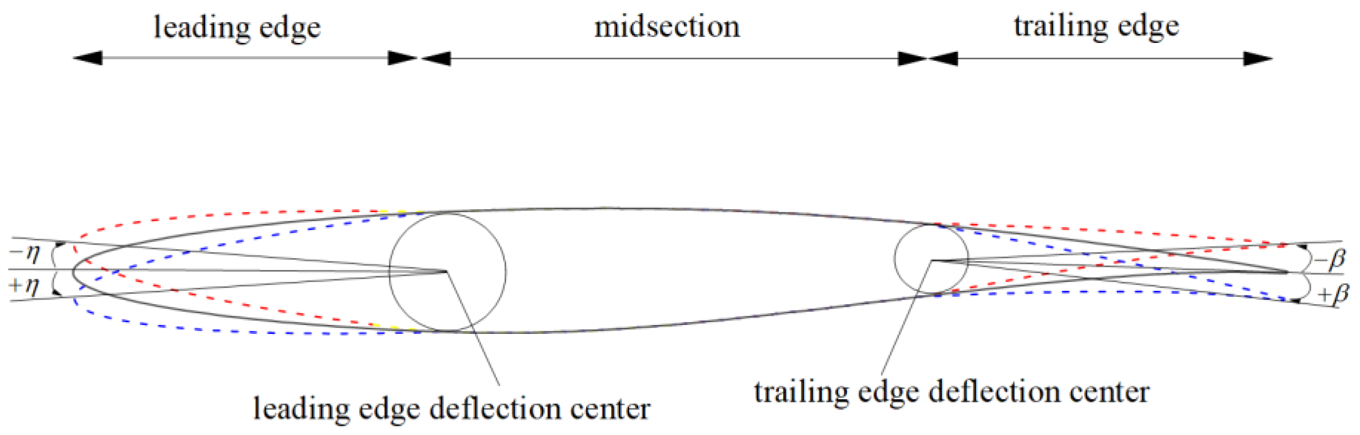
Figure 2.
Near-Wall CFD Mesh Model.
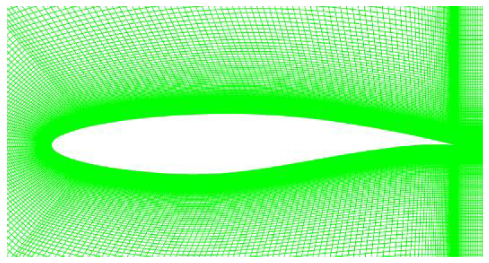
Figure 3.
Pressure Coefficient Curves for Different Grid Numbers.
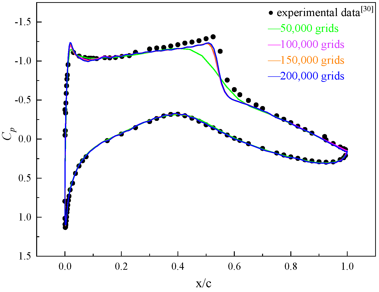
Figure 4.
Effect of Leading-Edge Deflection on the Aerodynamic Performance of Airfoils.
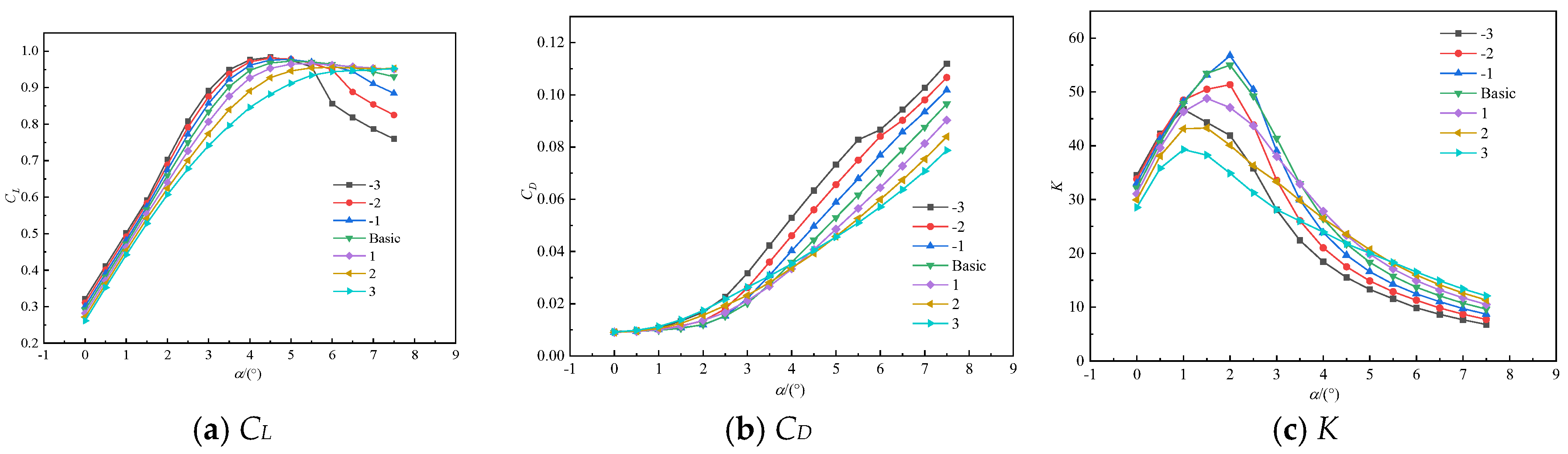
Figure 5.
Leading edge deflection pressure nephograms.
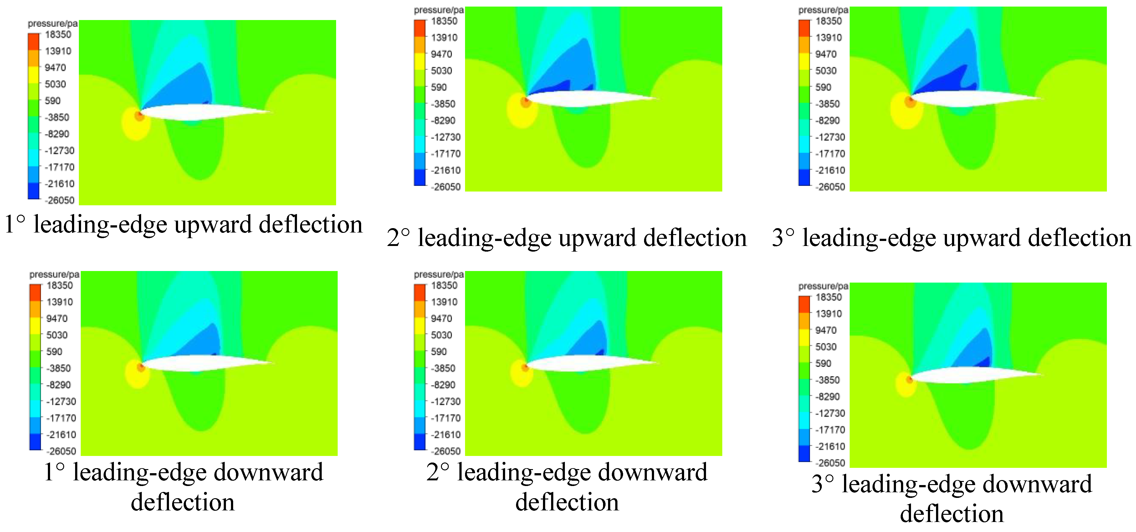
Figure 6.
Aerodynamic Performance of Leading Edge Deflection at Different Mach Numbers.
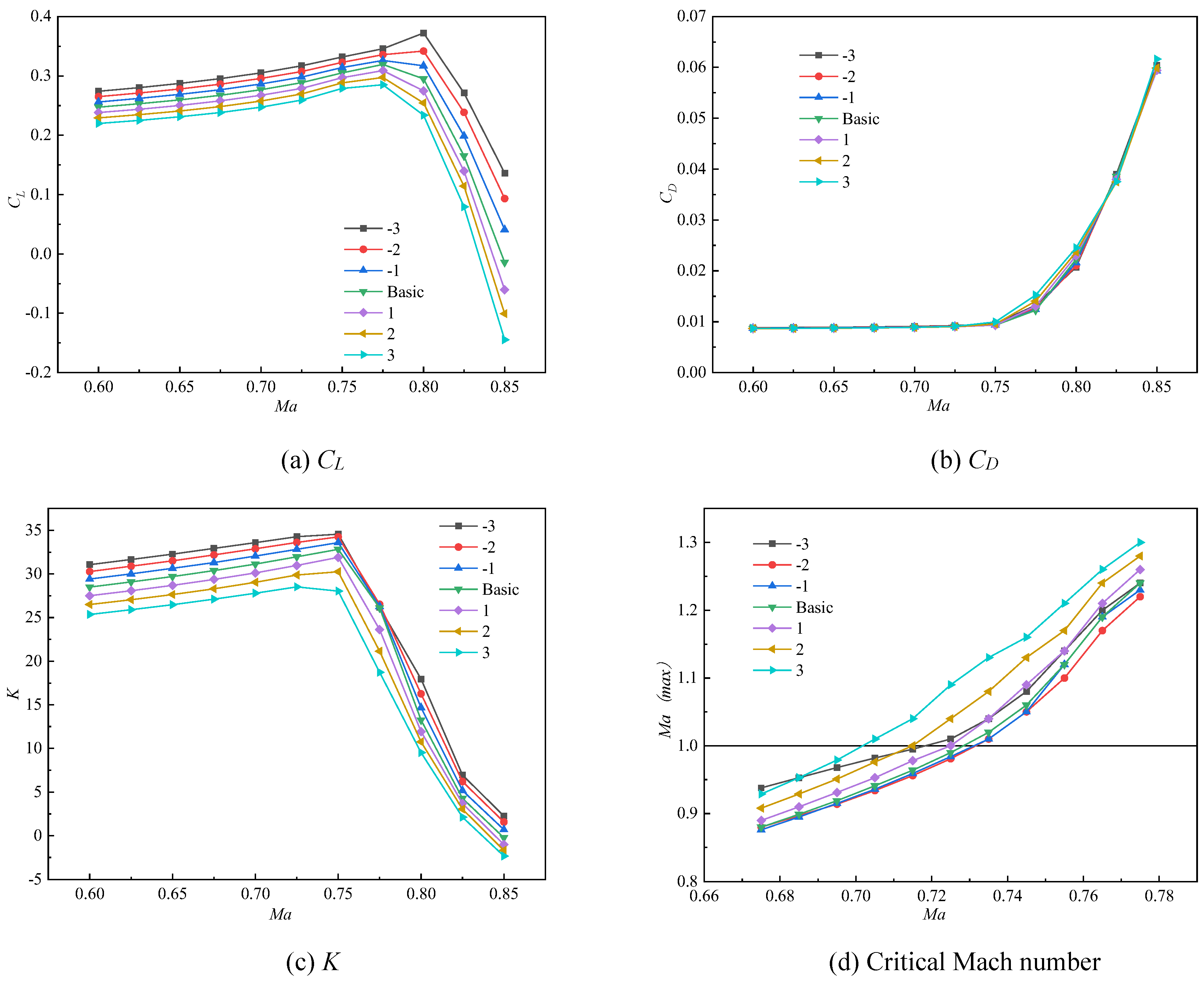
Figure 7.
Effect of Trailing-Edge Deflection on the Aerodynamic Performance of Airfoils.
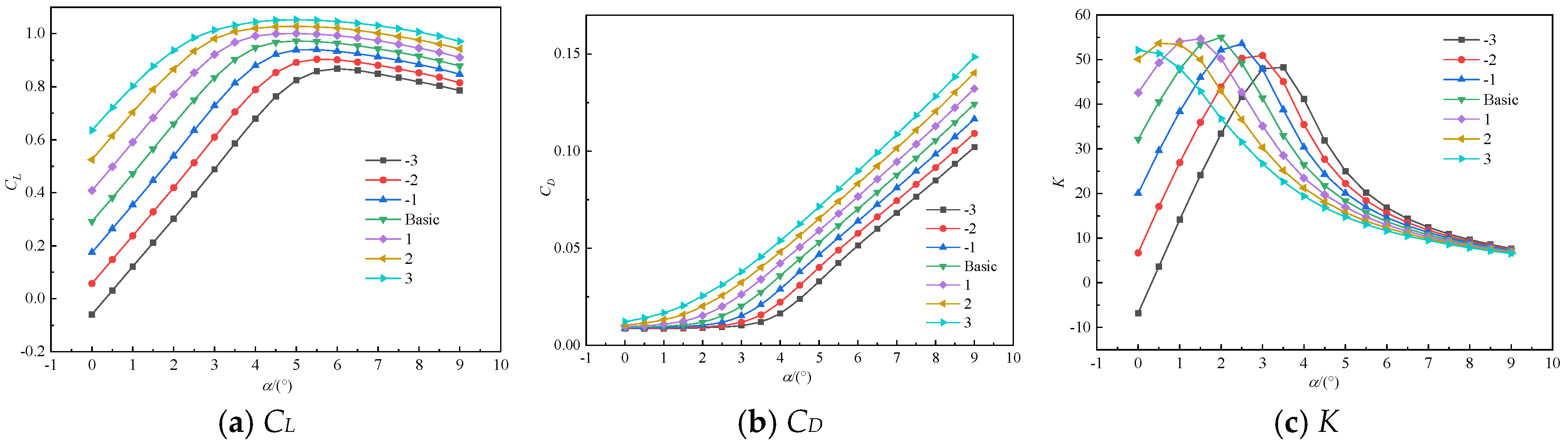
Figure 8.
Trailing edge deflection pressure nephograms.
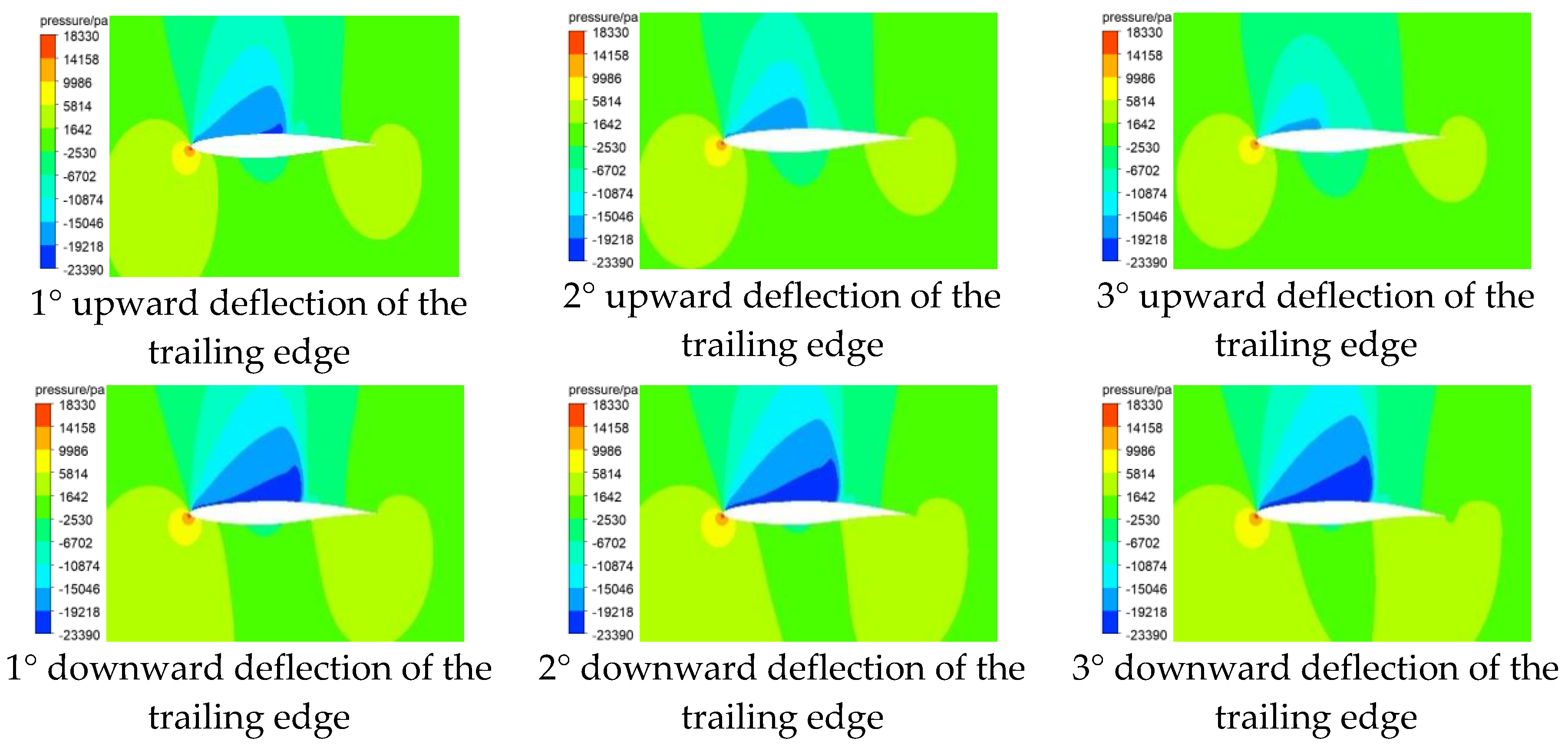
Figure 9.
Aerodynamic Performance of Trailing Edge Deflection at Different Mach Numbers.
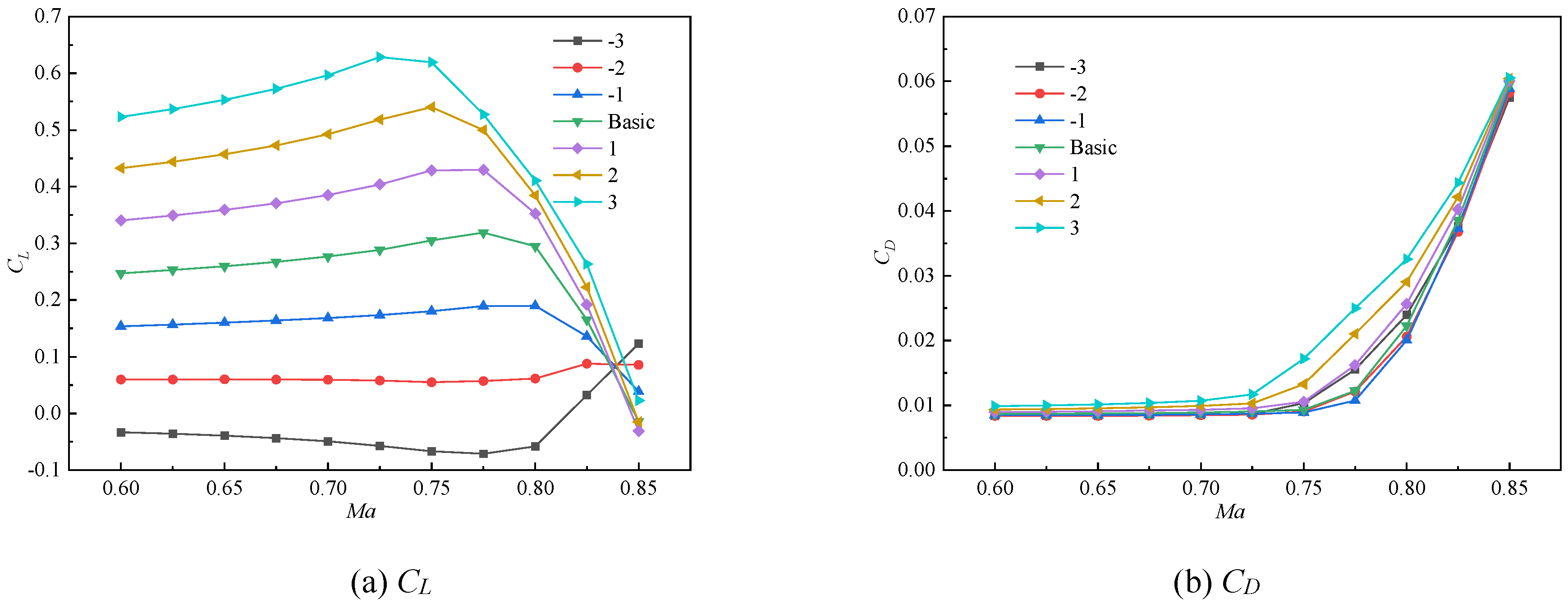
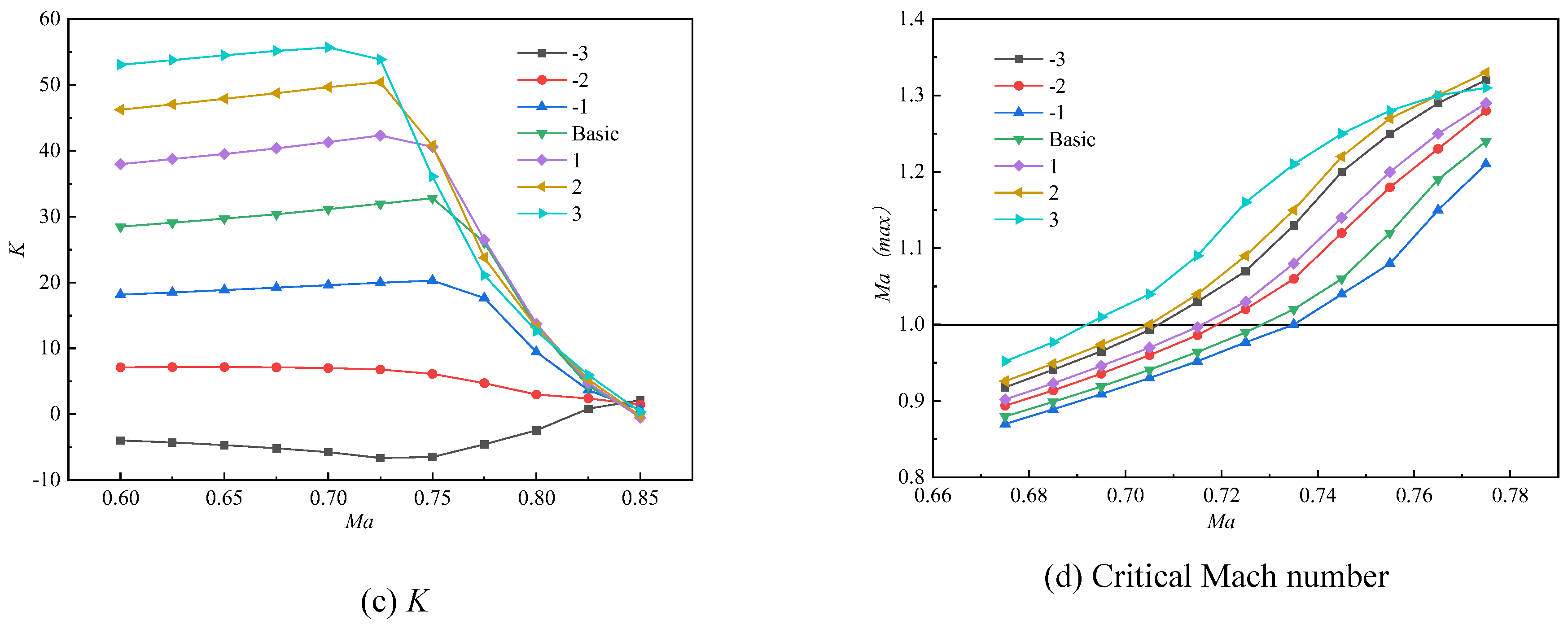
Figure 10.
Flowchart of Multi-Objective Optimization for Variable-Camber Airfoils.
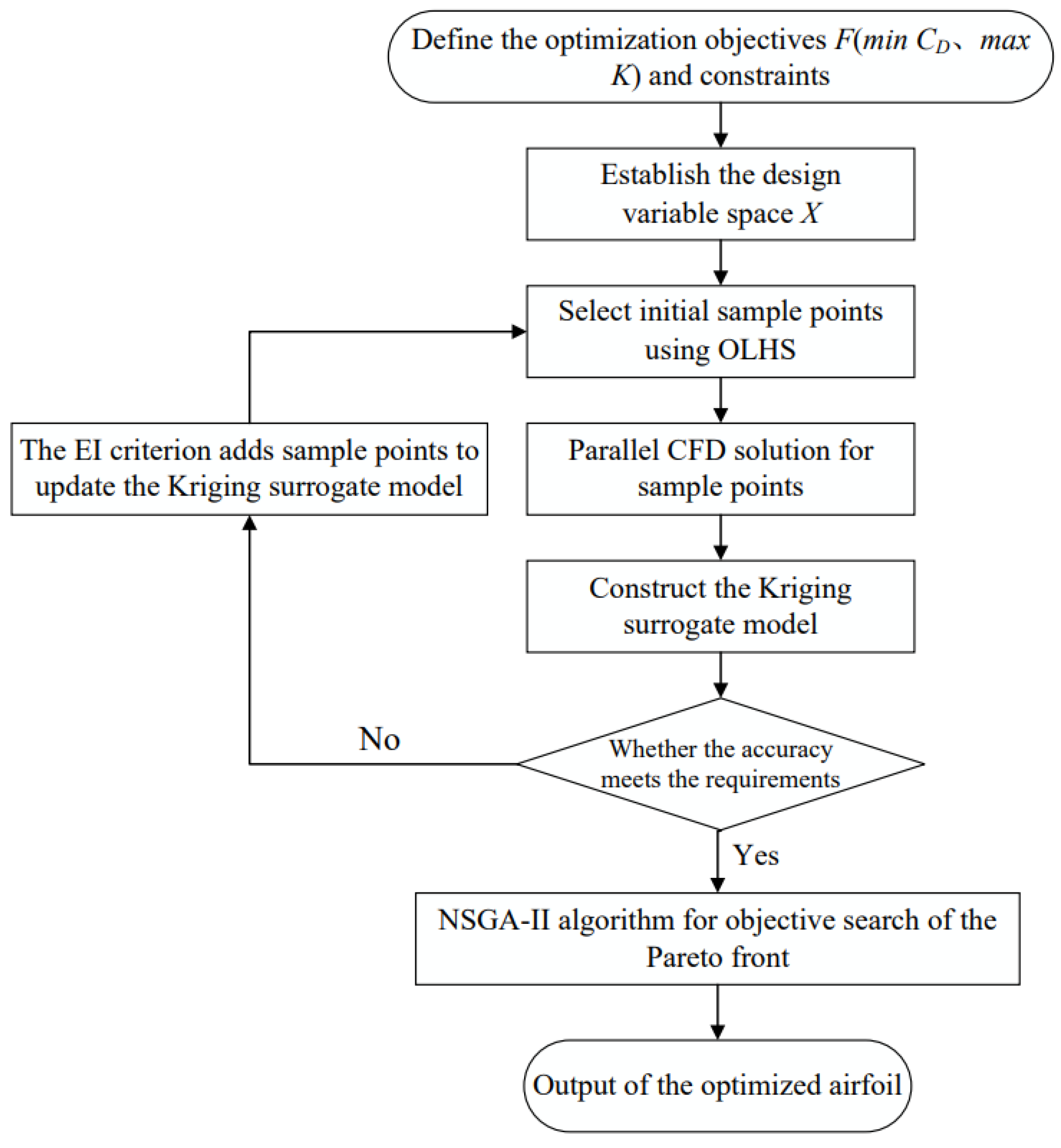
Figure 11.
Comparison of Two Sampling Designs.
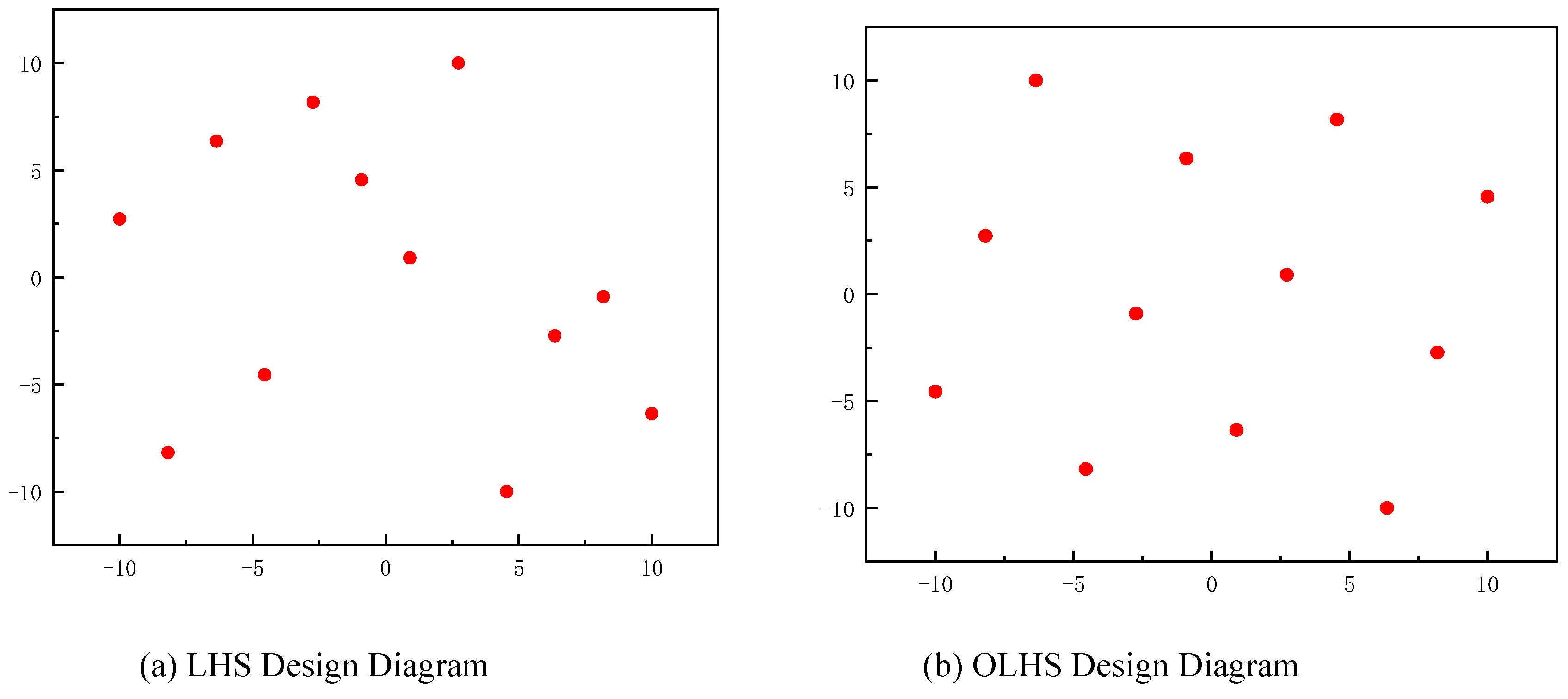
Figure 12.
Surrogate Model of Aerodynamic Coefficients and Fitting Validation Plot at Ma = 0.74.
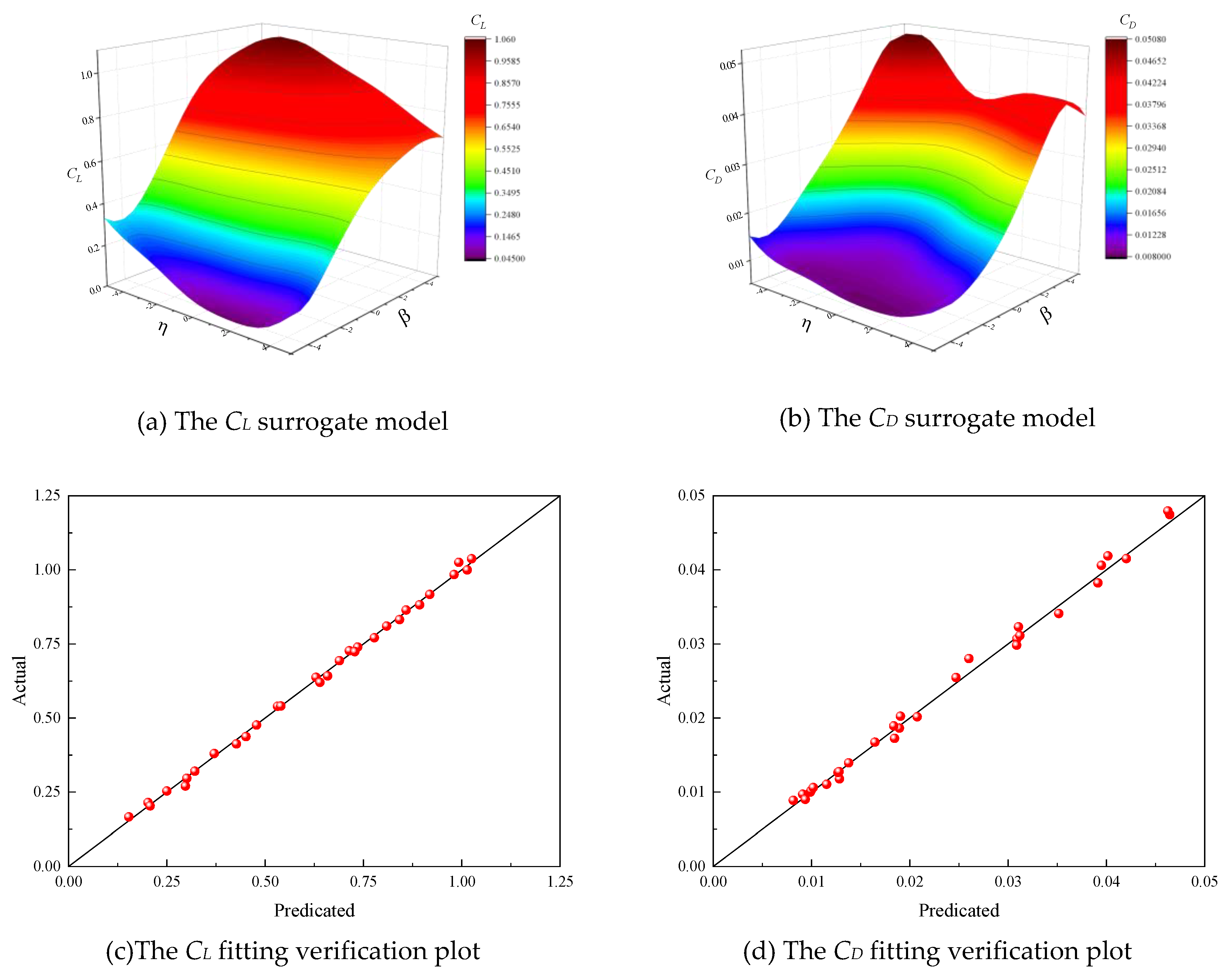
Figure 13.
Surrogate Model of Aerodynamic Coefficients and Fitting Validation Plot at Ma = 0.75.
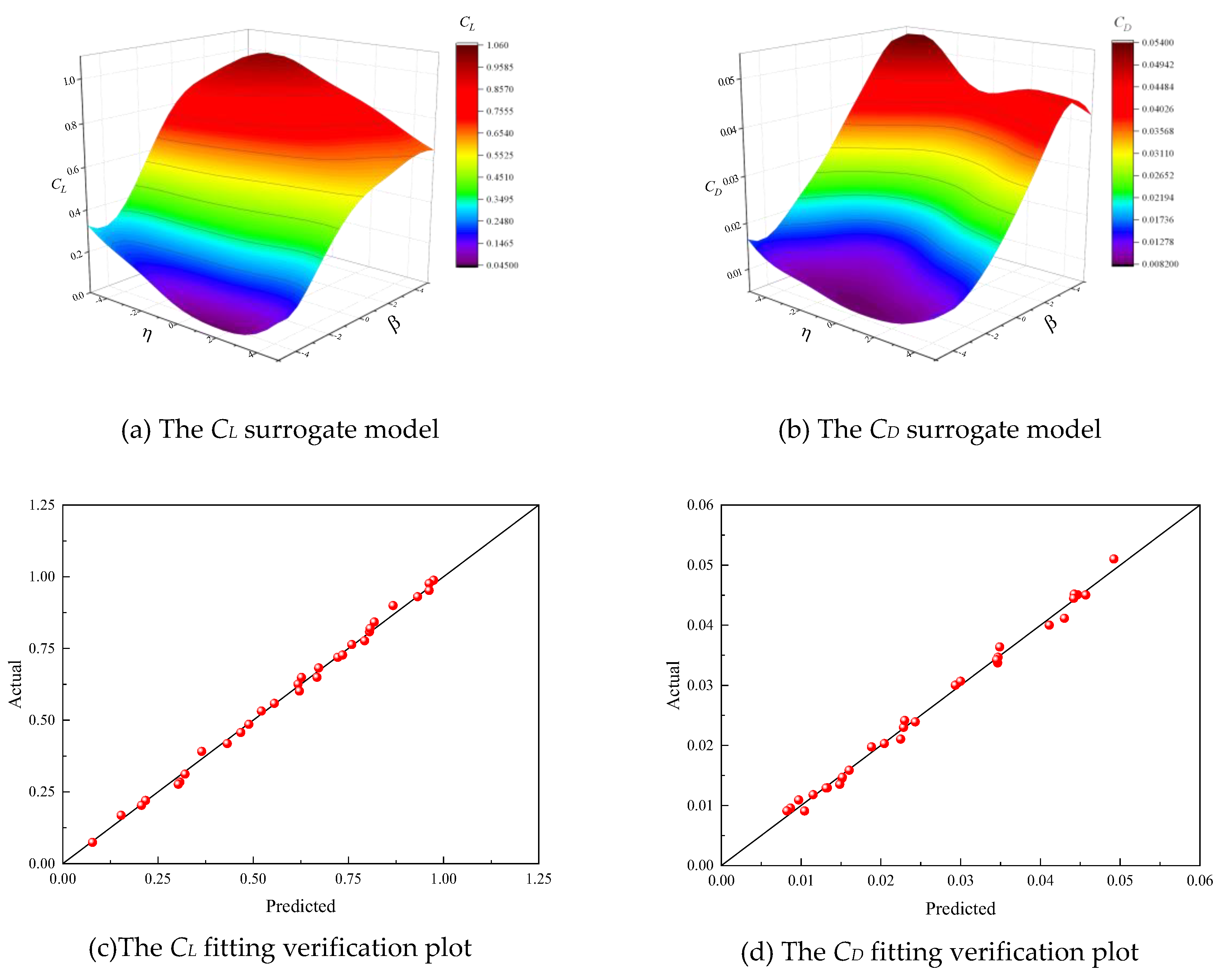
Figure 14.
Surrogate Model of Aerodynamic Coefficients and Fitting Validation Plot at Ma = 0.76.
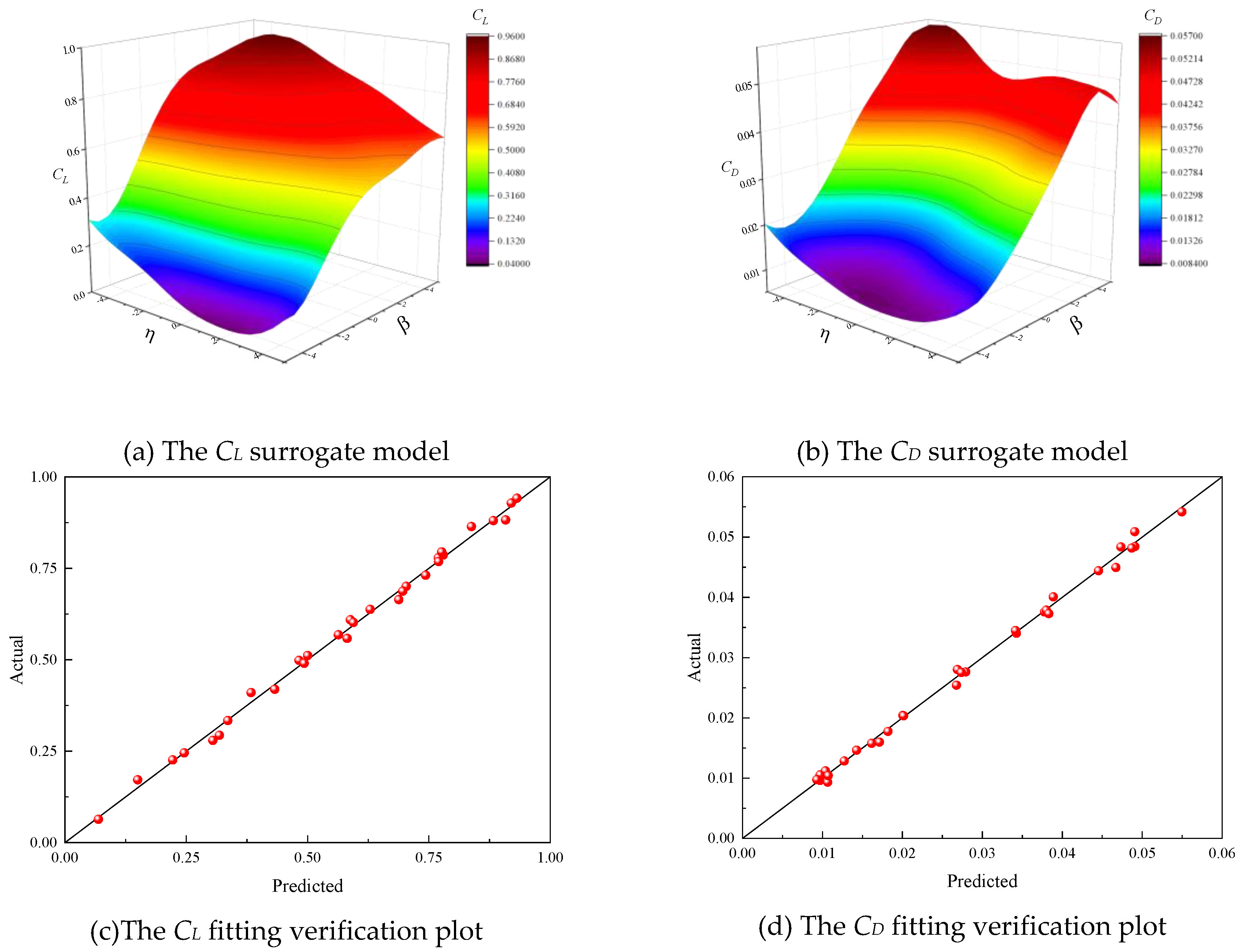
Figure 15.
Convergence Process (Ma = 0.74).
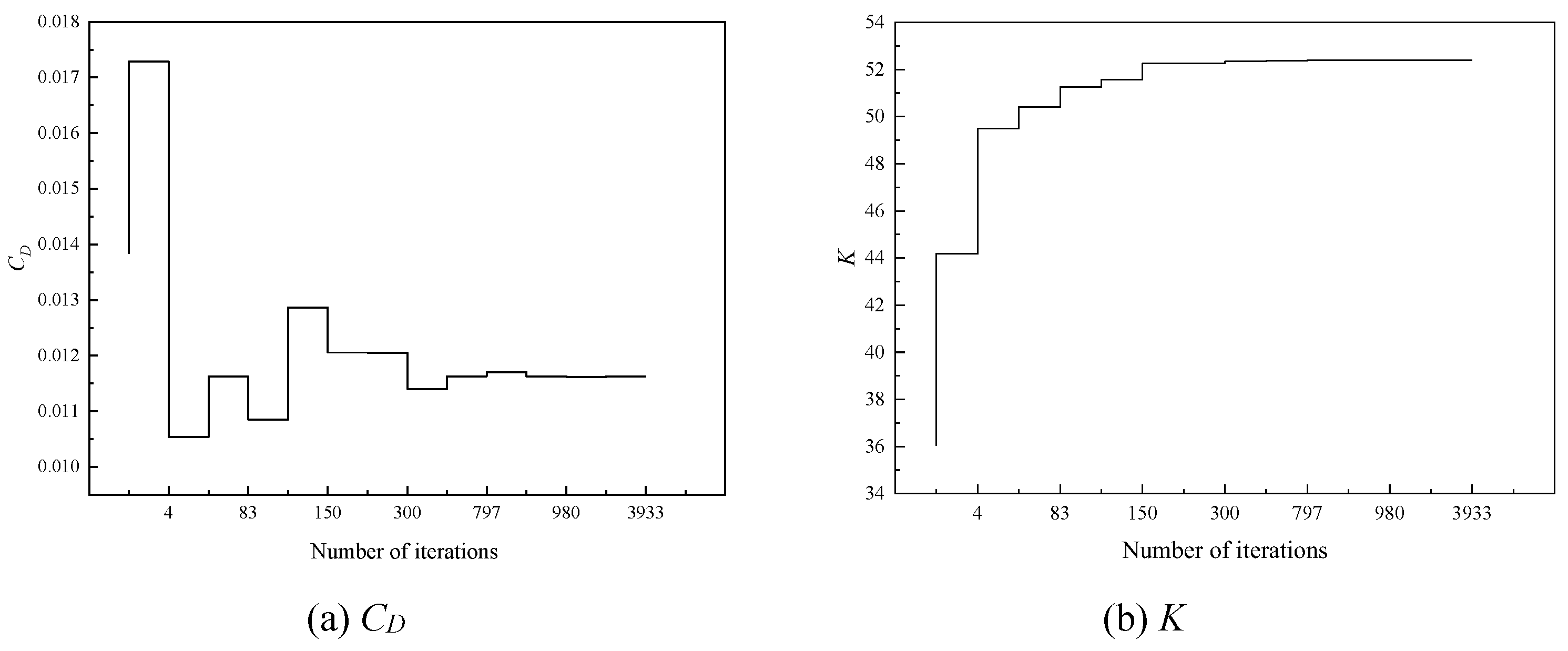
Figure 16.
Convergence Process (Ma = 0.75).
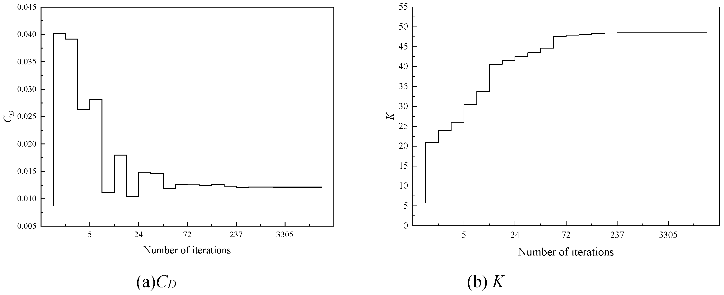
Figure 17.
Convergence Process (Ma = 0.76).
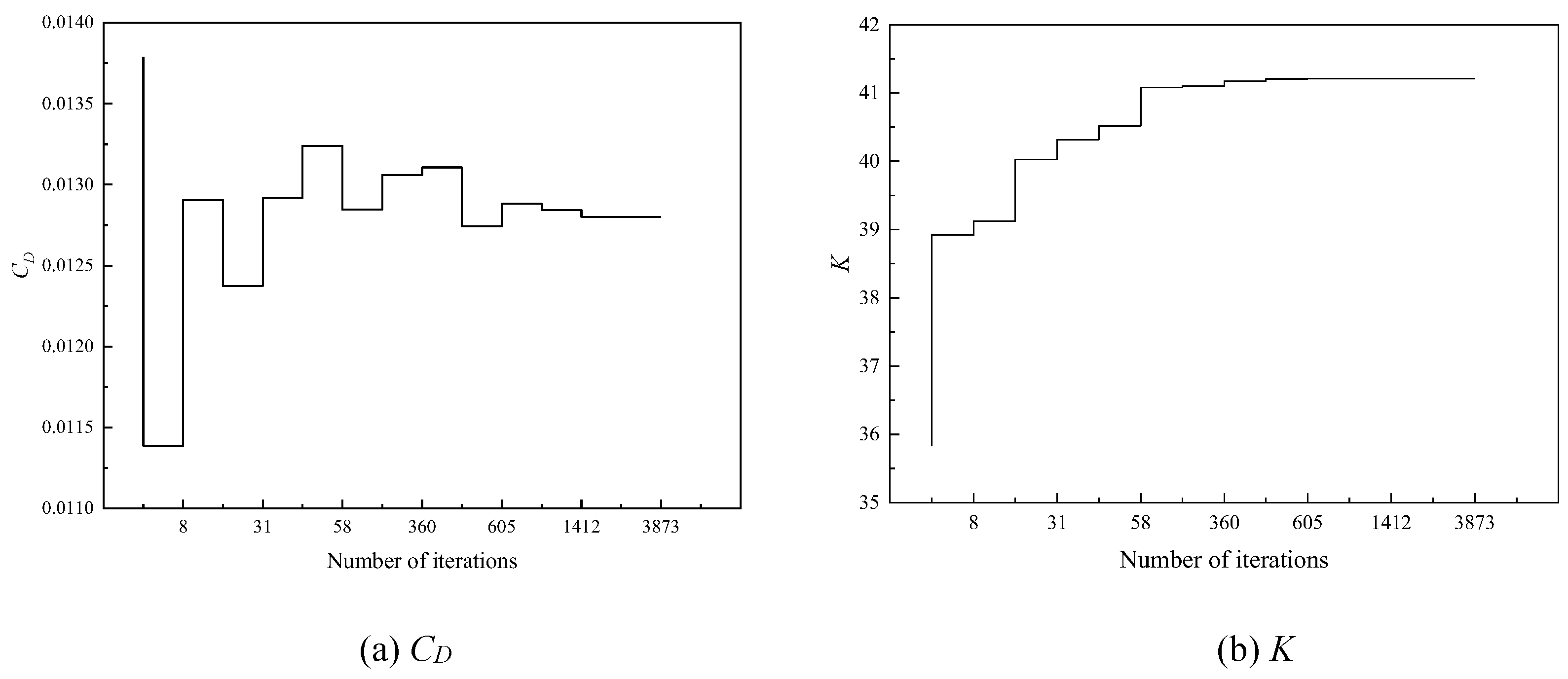
Figure 18.
Pareto Front.
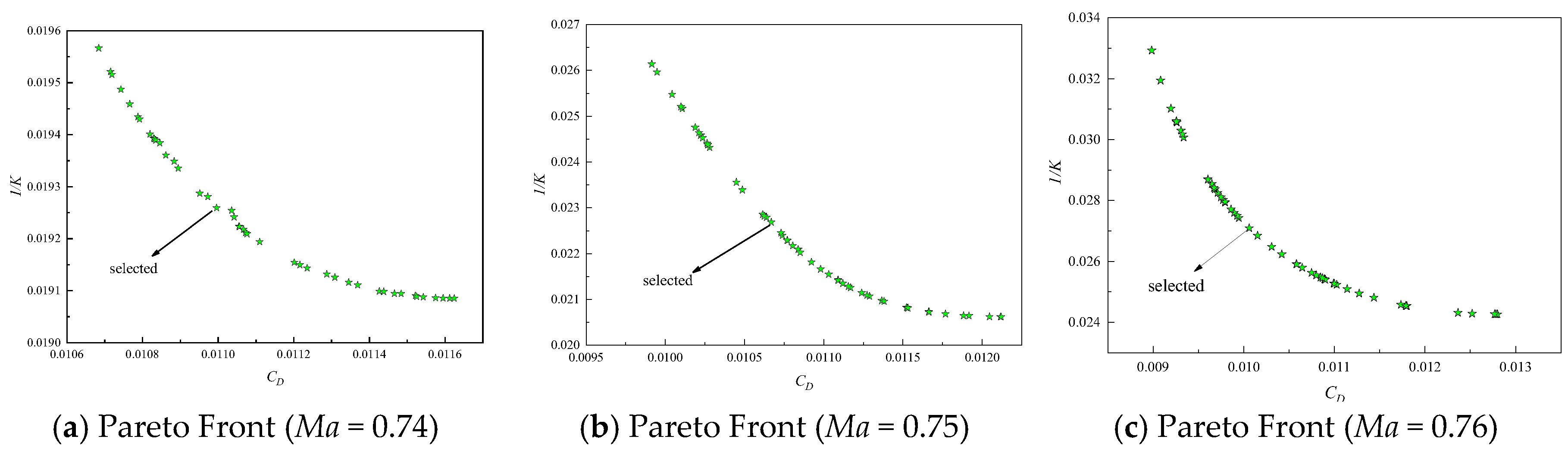
Figure 21.
pressure nephogram of the Airfoil Before and After Optimization.
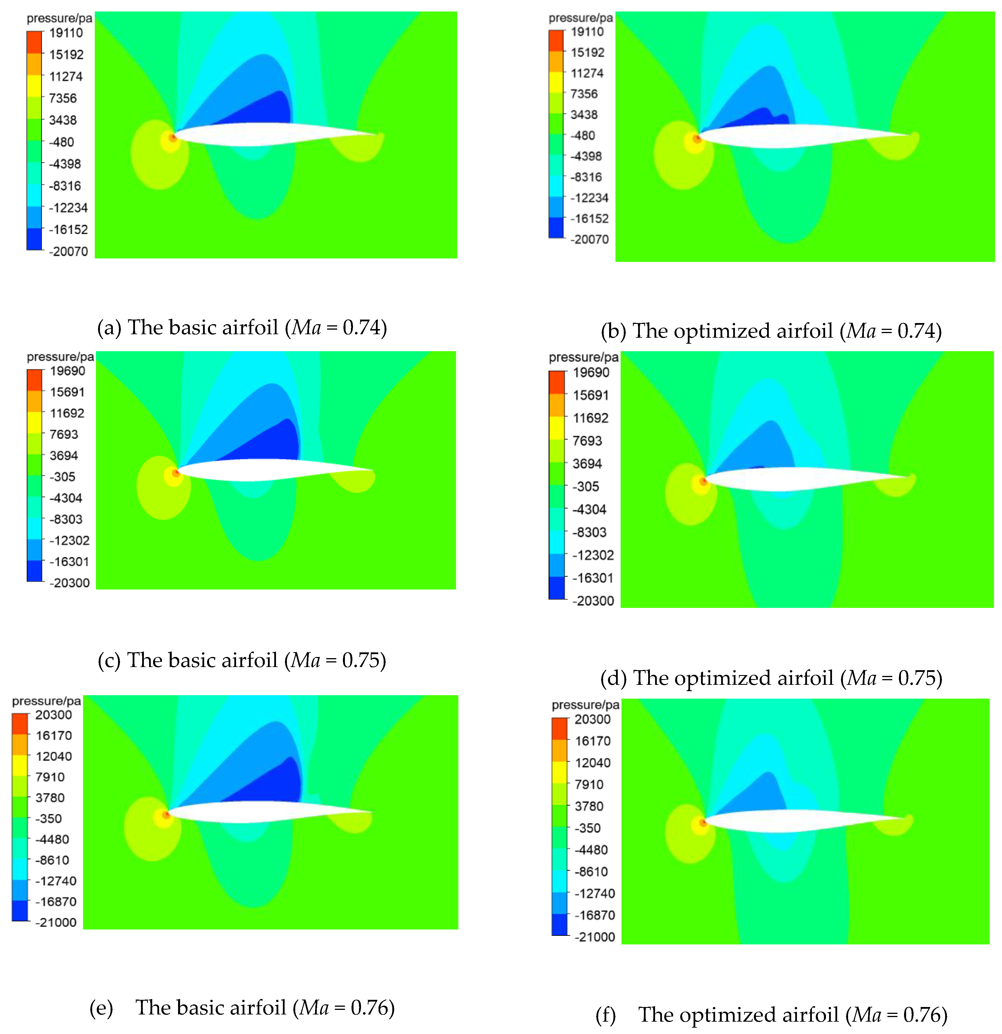
Figure 22.
Pressure Coefficient Curves of Basic Airfoil and Optimized Airfoil.
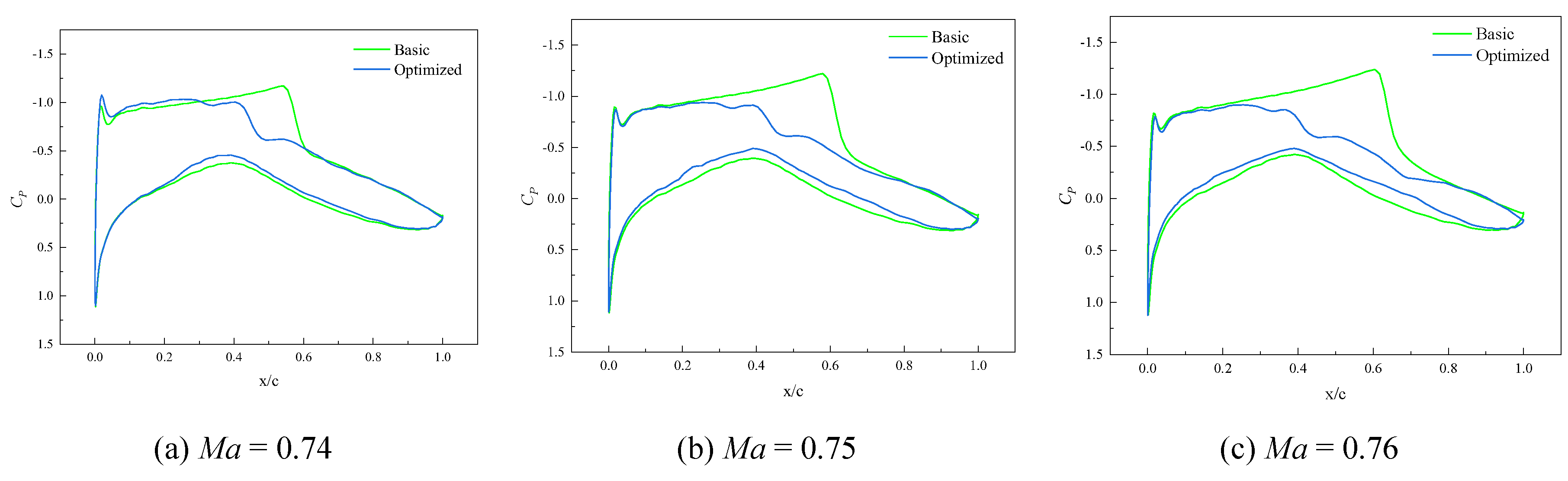

Table 1.
Aerodynamic Coefficients with Different Grid Resolutions.
| Number of grids | Lift coefficient CL | Drag coefficient CD | Pitching moment coefficient CM |
|---|---|---|---|
| Experiment [29] | 0.803 | 0.0168 | -0.099 |
| 50000 | 0.731279 | 0.016198 | -0.08786 |
| 100000 | 0.748625 | 0.016247 | -0.09152 |
| 150000 | 0.749577 | 0.016465 | -0.09343 |
| 200000 | 0.759939 | 0.016505 | -0.09389 |
Table 2.
Accuracy of Fitting for 30 Sampling Points.
| Flight Mach number | Types of Errors | Fit Accuracy of CL | Fit Accuracy of CD |
|---|---|---|---|
| Ma=0.74 | RMSE | 0.05614 | 0.06679 |
| R2 | 0.96384 | 0.9575 | |
| Ma=0.75 | RMSE | 0.05773 | 0.06787 |
| R2 | 0.96108 | 0.95705 | |
| Ma=0.76 | RMSE | 0.06099 | 0.06293 |
| R2 | 0.9551 | 0.96267 |
Table 3.
Optimization Results.
| Ma | Aerodynamic coefficients | Basic airfoil |
Surrogate model Optimization |
CFD Optimization | Surrogate model prediction error rate δ% | Improvement percentage ε % |
|---|---|---|---|---|---|---|
| 0.74 | CD | 0.0144 | 0.0110 | 0.0111 | 0.90 | -22.92 |
| K | 46.846 | 51.923 | 52.060 | 0.26 | +11.13 | |
| 0.75 | CD | 0.0180 | 0.0107 | 0.0101 | 5.94 | -43.88 |
| K | 37.636 | 44.077 | 45.409 | 2.93 | +20.65 | |
| 0.76 | CD | 0.0222 | 0.0101 | 0.0097 | 4.12 | -56.31 |
| K | 30.098 | 36.909 | 37.590 | 1.81 | +24.89 |
Disclaimer/Publisher’s Note: The statements, opinions and data contained in all publications are solely those of the individual author(s) and contributor(s) and not of MDPI and/or the editor(s). MDPI and/or the editor(s) disclaim responsibility for any injury to people or property resulting from any ideas, methods, instructions or products referred to in the content. |
© 2025 by the authors. Licensee MDPI, Basel, Switzerland. This article is an open access article distributed under the terms and conditions of the Creative Commons Attribution (CC BY) license (http://creativecommons.org/licenses/by/4.0/).
Copyright: This open access article is published under a Creative Commons CC BY 4.0 license, which permit the free download, distribution, and reuse, provided that the author and preprint are cited in any reuse.


