Submitted:
27 January 2025
Posted:
03 February 2025
You are already at the latest version
Abstract
Source apportionment and a more detailed understanding of local and remote contributions to the concentrations of greenhouse gases (GHGs) observed across WMO/GAW (World Meteorological Organization – Global Atmosphere Watch) stations can be achieved via proximity indicators and the implementation of new atmospheric tracers. In this study, the ratio between ozone (O3) and nitrogen oxides (NOx) is applied to nine continuous years (2015-2023) of measurements at the Lamezia Terme (LMT) observation site in Calabria, Southern Italy to differentiate the aging of air masses and identify four distinct categories: LOC (local), N–SRC (near source), R–SRC (remote source), and BKG (atmospheric background). Because of a possible overestimation of nitrogen di-oxide (NO2) caused by heated (~300-400 °C) molybdenum converters used in employed instru-ments, a correction factor based on a previous study has been integrated to further analyze the results. Additionally, this work introduces a new correction factor based on the local behavior of surface ozone and the diurnal peaks observed during boreal warm seasons in an area characterized by a Mediterranean climate. The results of this study confirm the hypotheses by previous works on local sources of pollution: the LOC category yields the highest concentrations observed at the site, which are in accordance with the northeastern wind sector and anthropogenic sources. R–SRC and BKG are more representative of atmospheric background levels and characterize westerly winds from the Tyrrhenian Sea. N–SRC, as expected, shows an intermediate behavior between local and remote/background levels.
Keywords:
greenhouse gases
; carbon monoxide
; carbon dioxide
; methane
; ozone
; nitrogen oxides
; GAW
; Mediterranean Basin
; Lamezia Terme
; Calabria
; proximity indicators
1. Introduction
In the field of Atmospheric Sciences, source apportionment and the evaluation of atmospheric tracers aimed at specific sources of emission have been, for decades, important tools toward a better understanding of atmospheric composition and its changes over time [1,2,3,4,5,6,7,8]. The atmosphere is a complex medium, and the lowermost layer is characterized by turbulent motion and kinetic interaction with the surface, which results in changes in the transport and concentration of greenhouse gases (GHGs) and aerosols [9,10,11,12,13,14,15]. In addition to these complexities, air masses can retain characteristics representative of their “aging”, i.e. whether air masses are fresh or linked to remote emission sources [16,17,18]. The findings of Parrish et al. (2009) [19] and Morgan et al. (2010) [20] demonstrated that the ratio between ozone (O3) and nitrogen oxides (NO + NO2 = NOx) could be used as a “proximity indicator” and consequently differentiate local emissions from remote/background outputs. A high O3/NOx ratio would be attributable to aged air masses, while a low ratio would be considered linked to local sources of emissions. In the atmosphere, NOx are an important control factor over O3 [21,22,23,24,25,26,27,28] and are generally linked to anthropogenic sources such as fossil/biomass burning and fertilizer use in agricultural activities [29,30,31,32,33,34]. O3 is of anthropogenic and natural origin [35,36] and is differentiated in two categories: stratospheric O3, which is beneficial for Earth’s ecosystem thanks to its capacity to partially screen the surface from solar ultraviolet (UV) radiation [37,38,39], and tropospheric O3, which poses health and environmental hazards [40,41,42,43,44]. This information, combined with additional atmospheric tracers and indicators of specific emission sources, can provide an accurate understanding of anthropogenic and natural emissions, which in turn can further improve regulations and mitigation strategies at local-to-global scales [45,46,47,48].
Prior to these findings, a study by Steinbacher et al. (2007) [49] demonstrated that heated molybdenum converters (~300-400 °C) used in instruments commonly employed for NOx measurements can significantly overestimate (~50%) observed NO2 mole fractions. Specifically, other nitrogen species such as nitric acid (HNO3), nitrous acid (HONO), nitric acid anhydride (N2O5), ethyl nitrate (C2H5NO3) and peroxyacetyl nitrate (C2H3NO5, or PAN) can interfere with NO2 measurements and provide inaccurate readings. With oxygen (O2), NO2 is reduced to NO and the converter’s surface is oxidized to molybdenum trioxide (MoO3) or dioxide (MoO2). Over time, many studies highlighted the possibility of organic nitrates reduction to NO under specific conditions [50,51,52,53]. The interference is believed to be amplified in aged air masses, characterized by a high O3/NOx ratio [49]. In literature, the issues posed by the measurement of “true NOx” concentrations have been the subject of various papers focused on different methodologies and ways to determine the extent of uncertainties in NOx [54,55,56,57]; these studies are often based on comparisons between different instruments and methods meant to test errors in measurements caused by heated molybdenum converters and similar devices [58,59].
At the Lamezia Terme (code: LMT) WMO/GAW (World Meteorological Organization – Global Atmosphere Watch) observation site in Calabria, Southern Italy, an early study based on preliminary data gathered at the observatory relied on O3/NOx ratio thresholds as proximity indicators to differentiate local-to-remote sources of emissions and also accounted for possible NO2 overestimation by applying a correction factor [60]. In this study, nine years of continuous measurements (2015-2023) have been evaluated to further expand the knowledge gathered by preliminary findings and provide the most accurate differentiation between local and remote sources ever performed at the site. This study also proposes a new correction factor based on the local behavior of ozone at LMT as described in D’Amico et al. (2024d) [61].
Three compounds will be evaluated in this paper, based on proximity categories: carbon monoxide (CO), carbon dioxide (CO2), and methane (CH4). CH4 was subject to a detailed multi-year (2016-2022) study assessing its variability and patterns [62] while CO and CO2 have been assessed in their multi-year variability mostly with respect to weekly cycles and the influence of anthropogenic activities on seasonal concentrations [63].
Due to its nature as a combustion byproduct, CO is an ideal target gas to assess anthropogenic emissions, especially those attributable to domestic heating and fuel burning [64,65,66]. Its short lifetime in the atmosphere (~60 days) [67] allows it to be used, in conjunction with the proximity indicators employed in this paper, as an effective tracer of local anthropogenic emissions. It is worth mentioning that CO is not a greenhouse gas per se, as it does not contribute to Earth’s radiative forcing perturbation; however, it plays an important role in atmospheric chemistry via its effects on other compounds which do have an impact on the global climate [68,69]. This compound has been on the rise for decades [70], but emission mitigation policies and the optimization of engines managed to counterbalance the effect [71]; major wildfires are however deemed responsible for recent increases in atmospheric CO concentrations [72,73].
CO2 is the key driver of anthropogenic climate change [74,75,76,77,78], which is amplified by a long atmospheric lifetime (~1.000 years) [79]. Fossil fuel burning is the primary source of anthropogenic CO2 [80] and the mitigation of these emissions are one of the most notable challenges in climate change policies and regulations. Due to its long lifetime, observed CO2 may not be susceptible to major changes between evaluated proximity categories as both aged and fresh air masses would be characterized by similar CO2 concentrations. However, via proximity categories, a differentiation between fresh anthropogenic outputs and the atmospheric background – which is susceptible to global anthropogenic emissions – should be possible. Atmospheric CO2 has been on the rise for decades due to anthropogenic emissions: observatories such as the Mauna Loa site operated by NOAA (National Oceanic and Atmospheric Administration) provide accurate information on the upward trend caused by anthropic activities [81,82].
With an intermediate lifetime between CO and CO2, CH4 (~10 years) [83,84,85] is characterized by a GWP (Global Warming Potential) which is nearly two orders of magnitude higher than that of CO2 [86]. CH4 is a combustion byproduct [87,88,89] but is most notably released by wetlands and other natural sources [90]. Livestock farming and landfills are among the key anthropogenic emissions of this compound [91]. Like CO2, CH4 is characterized by an upward trend driven by anthropogenic emissions but its mechanisms and chemistry are affected by an articulated balance of sources and sinks: in fact, the analysis of stable carbon isotopes has allowed to determine a shift in biogenic/anthropogenic balances of atmospheric CH4 [92].
2. Instruments, Datasets, and Methodologies
At Lamezia Terme (LMT), key data on wind (speed and direction) were gathered by a Vaisala WXT520 (Vantaa, Finland) instrument. The WXT520 performs its measurements of wind speed (WS, in m/s) and direction (WD, in degrees) via ultrasounds transmitted between three transducers on a horizontal plane. Wind from a given direction and at a given speed alters the time required for ultrasound pulses to travel between the transducers; the instrument measures the deviation from a standard travel time and calculates WS and WD with a precision of 0.3 m/s and 3°, respectively. In addition to WS and WD, the instrument measures meteorological parameters such as temperature and relative humidity. Further details on Vaisala WXT520 measurements and data processing at LMT are available in D’Amico et al. (2024c) [93].
The mole fractions of carbon monoxide (ppb), carbon dioxide (ppm), and methane (ppb) at the site have been measured by a Picarro G2401 CRDS (Cavity Ring-Down Spectrometry). CRD spectrometry allows the measurement, with high degrees of precision, of greenhouse gases in the atmosphere [94]. In accordance with NOAA procedures, the Picarro G2401 operating at LMT is subject to frequent calibration via cylinders based on WMO standards. In addition to WMO cylinders, other target cylinders are used for quality assurance purposes. Details on G2401 measurements and data processing at LMT are available in D’Amico et al. (2024a) [62] and D’Amico et al. (2024c) [93].
Nitrogen oxides have been measured by a Thermo Scientific 42i (Franklin, Massachusetts, USA). The instrument operates under the principle of chemiluminescence (CL) by which NO in ambient air reacts with O3 produced by the instrument itself to release NO2 in an excited state, and molecular oxygen (O2) [95]. More details on NOx measurements at LMT are available in Cristofanelli et al. (2017) [60] and D’Amico et al. (2024c) [93]. The instrument is equipped with a molybdenum converter which can overestimate NO2, as described in Section 1.
The concentrations of surface ozone have been measured by a Thermo Scientific 49i (Franklin, Massachusetts, USA) operating as a photometric analyzer. The 49i uses Lambert’s Law, combined with O3’s absorption of ultraviolet light at a wavelength of precisely 254 nanometers. Via a two-cell mechanism, sampled ambient air and a reference depleted in O3 by a scrubber are used to calculate O3 concentrations. A detailed description of these measurements at LMT is available in D’Amico et al. (2024d) [61].
Table 1 shows the coverage of all four instruments throughout the observation period (2015-2023) and the applicability of proximity indicators to analyzed parameters.
Proximity categories have been calculated using the same thresholds from the previous study, which was aimed at LMT and other southern Italian stations [60]. The local (LOC) category has been defined with a O3/NOx ratio lower than or equal to 10; the near source (N–SRC) has been set with a 10 < O3/NOx ≤ 50 ratio; for remote source (R–SRC) emissions, the 50 < O3/NOx ≤ 100 ratio was used; finally, for background (BKG) air masses, the category was defined with a ratio greater than 100.
Corrections for remote source (R–SRC) and atmospheric background (BKG) categories had already been calculated in the previous study according to the findings of Steinbacher et al. (2007) [49] on the overestimation of NO2 in aged air masses. Consequently, for R–SRC and BKG thresholds, NO2 concentrations have been divided by two to generate the “corrected” S-SRCcor and BKGcor subcategories as per the methodology seen in Cristofanelli et al. (2017) [60].
Following the analysis of surface ozone at the LMT site performed in D’Amico et al. (2024d) [61] which demonstrated the occurrence of diurnal peaks of O3 linked to warm seasons and westerly winds from the Tyrrhenian Sea, in this study an additional correction is proposed and consequently applied. The purpose of this correction is to compensate for the peaks of O3 linked to heavy photochemical activity under specific circumstances, which would cause fresh air masses to fall under more aged categories instead. For this purpose, “ecor” (for “enhanced correction”) divided O3 concentrations by two when all of the following conditions were satisfied: a) measurement occurring during a warm season, i.e. Spring and Summer (March to August); b) diurnal hours, i.e. between 10:00 and 16:00 UTC; c) westerly winds, i.e. wind directions between 240 and 300 °N. An R 4.4.2 algorithm based on the dplyr package and library has been used to apply the correction under the circumstances specified above.
Table 2 reports the rate of hours falling into each category, by year, as subsets of the “Preliminary” dataset shown in Table 1 which does not account for Picarro G2401 and Vaisala WXT520 coverages.
As evidenced by the previous work [60], the implementation of a correction meant to compensate for molybdenum converters’ overestimation of NO2 results in a reduction of R–SRC and an increase of BKG. The O3 correction applied in this study has an opposite behavior, although corrected R–SRC data are still lower compared to their standard counterparts. Direct comparisons between standard and corrected values are shown in Table 3.
In this study, both the standard and corrected values are used, however the latter (especially “ecor”) are excluded from a number of graphs to optimize visualization. Seasonal averages have been calculated by assigning the following months to each season, in accordance with previous research [60,61,62]: January, February, and December to Winter (JFD); March, April, and May to Spring (MAM); June, July, and August to Summer (JJA); September, October, and November to Fall (SON). Weekly analyses are based on the methodology seen in D’Amico et al. (2024b] [63]. Monthly aggregations have also been calculated. All data have been processed in R 4.4.2 and plots showing the results of these evaluations have been generated with the following packages and libraries: ggplot2, ggpubr, tidyverse. Polar plots have been computed in MATLAB2016a using the datasets processed in R.
3. Characteristics of the Lamezia Terme WMO/GAW Observation Site
Located in the southern Italian region of Calabria and operated by CNR-ISAC (National Research Council of Italy – Institute of Atmospheric Sciences and Climate, the Lamezia Terme (code: LMT; Lat: 38°52.605′ N; Lon: 16° 13.946′ E; Alt: 6 m ASL) WMO/GAW (World Meteorological Organization – Global Atmosphere Watch) regional observation site is 600 meters from the Tyrrhenian coast of the region, in the narrowest point of the entire Italian peninsula (Figure 1). The distance between the western (Tyrrhenian) and eastern (Ionian) coasts is ≈32 kilometers, and the entire area – known as Catanzaro isthmus, after the regional capital of the region located in the eastern coast – separates the Sila Massif and coastal chain (Catena Costiera) in the north from the Serre Massif in the south. The station started data gathering operations in 2015 and has since been performing continuous measurements of gases and aerosols in the atmosphere, as well as meteorological data.
The orographic configuration of the area, combined with LMT’s location in the westernmost area of the isthmus, results into the site being affected by a well-defined wind pattern. Prior to gas and aerosol measurements, a number of studies allowed to characterize the area with respect to wind circulation. Federico et al. (2010a) [96] demonstrated the importance of breezes as a key regulating factor in local wind circulation and climate: breeze regimes vary depending on the season, and minor changes in wind orientations are also observed. However, the W-WSW/NE-ENE axis dominates throughout the entire year as a result of local orography and wind channeling through the Marcellinara gap in the Catanzaro isthmus (Figure 1). When considering the 850 hPa layer however, northwestern winds prevail in accordance with the large scale circulation in the area. In Federico et al. (2010b) [97] two years of data have been assessed and modeled to provide a more accurate understanding of wind regimes. The study demonstrated that during part of fall, spring, and summer, diurnal breezes are the result of a combination between large-scale and local flows, while in November and winter, diurnal circulation is linked to large-scale forcing. According to the study, nocturnal flows are linked to nocturnal breeze circulation.
Data from a short campaign, limited to measurements performed during summer 2009, were used to analyze PBL (Planetary Boundary Layer) variability at the site [98,99]. The characterization of near-surface wind patterns was the subject of additional studies which used wind lidars and other instruments to characterize the behavior of local winds at various altitude thresholds [100].
Following the implementation of GHG and aerosol measurements, research focused on data gathered at the site and their evaluation. In Cristofanelli et al. (2017) [60], preliminary data from LMT and other stations in southern Italy have been used to assess local and remote sources contributing to observed atmospheric concentrations of select gases. The study, which relied on the O3/NOx ratio as proximity indicator, showed that LOC (local) concentrations of methane at the site were higher than their remote counterparts and indicated livestock farming in the area as a possible cause for these emissions. In addition to these outputs, other sources of pollution were identified in the preliminary study: the Lamezia Terme International Airport (IATA: SUF; ICAO: LICA) located 3 km north from the observatory, and the A2/E45 highway (Figure 1). It is worth mentioning that the runway of the airport has a 100°N/280°N (RWY 10/28) orientation which results into local air traffic being oriented on the same wind axes observed at the LMT site.
A multi-year study on methane, based on seven years of continuous measurements (2016-2022), described in greater detail the behavior of this compound at LMT [62]: methane concentrations are lower in the western-seaside sector, and higher in the northeastern-continental sector due to the influence of anthropogenic sources. Furthermore, the study demonstrated the occurrence of a HBP (Hyperbola Branch Pattern) linked to the northeastern sector: methane concentrations tend to be higher in the presence of low wind speeds, and vice versa, high wind speed is generally linked to low methane concentrations. The second compound to be subject to a detailed multi-year and cyclic analysis at LMT is ozone: in D’Amico et al. (2024d) [61], nine years (2015-2023) of measurements have characterized surface ozone’s behavior at LMT and demonstrated the effect of photochemical activity over warm season peaks observed from the western sector. The findings demonstrated that the behavior over the W/NE axis varies depending on the nature of each compound; the northeastern sector – which is exposed to more anthropogenic pollution – is not always linked to peaks in observed compounds. The same results have been used in this study to apply the “ecor” correction of surface ozone under precise conditions.
A study performed on data gathered during the first COVID-19 lockdown of 2020, during which strict regulations were introduced by the Italian government with the effect of stopping, or reducing, most anthropic activities [102,103], assessed the variability of greenhouse gases and aerosols via a comparison between pre-lockdown, lockdown, and post-lockdown concentrations [93]. The study showed radical changes in the behavior of nitrogen oxides in particular, thus demonstrating that the peaks observed at LMT during rush hours were attributable to vehicular traffic, as hypothesized in a previous study [60].
More complexity in the behavior of gases and aerosols at the site was described following a May-September 2024 campaign pairing surface observations of these parameters with PBLH (Planetary Boundary Layer Height) variability measured by a Lufft CHM 15k Nimbus ceilometer (Fellbach, Germany) [15]. Ceilometer data, in conjunction with Vaisala WXT520 measurements of wind speeds and directions, allowed to define four distinct wind regimes at the site, each with peculiar characteristics in terms of GHG and aerosol concentrations.
Due to its location in the central Mediterranean (Figure 1), LMT is exposed to frequent Saharan dust events from Africa [104], and open fire emissions from sources ranging from regional to continental [105]. In particular, the latter contribute with carbon monoxide anomalies during the summer season, which are distinct from the peaks observed in winter, attributed to domestic heating and other forms of biomass burning.
4. Results
4.1. CO, CO2, and CH4 Concentration Variability by Category
Using the four standard proximity categories and the corrected (cor, ecor) concentrations, CO (ppb), CO2 (ppm), and CH4 (ppb) data have been aggregated on a per-category basis to assess possible differences. The results, shown in Table 4, are based on the “Proximity” dataset combining CO, CO2, CH4, O3, and NOx measurements from three distinct instruments (Picarro G2401, Thermo 49i, Thermo 42i).
4.2. Assessment of Daily Cycles
At LMT, studies have shown the presence of daily cycles which are the result of local wind circulation, seasonal changes, and atmospheric chemistry [60,61,62,93]. Of the three compounds assessed in this study, only methane was subject to a detailed daily cycle analysis [62]. In this subsection, proximity categories are introduced as a new variable to assess their influences on the daily cycle of carbon monoxide (Figure 3), carbon dioxide (Figure 4), and methane (Figure 5) on a seasonal basis. In order to optimize visualization, “ecor” data are featured in R–SRCcor (E) and BKGcor (F) plots as dashed lines.
4.3. Weekly Cycle Variability
In the multi-year assessment of methane at LMT based on seven years of data (2016-2022) [62], weekly evaluations were performed. These were further expanded in D’Amico et al. (2024b) [63], which introduced new methods for weekly analyses. In this study, weekly cycles have been assessed to test the influences of anthropogenic emissions especially in the case of LOC and N–SRC.
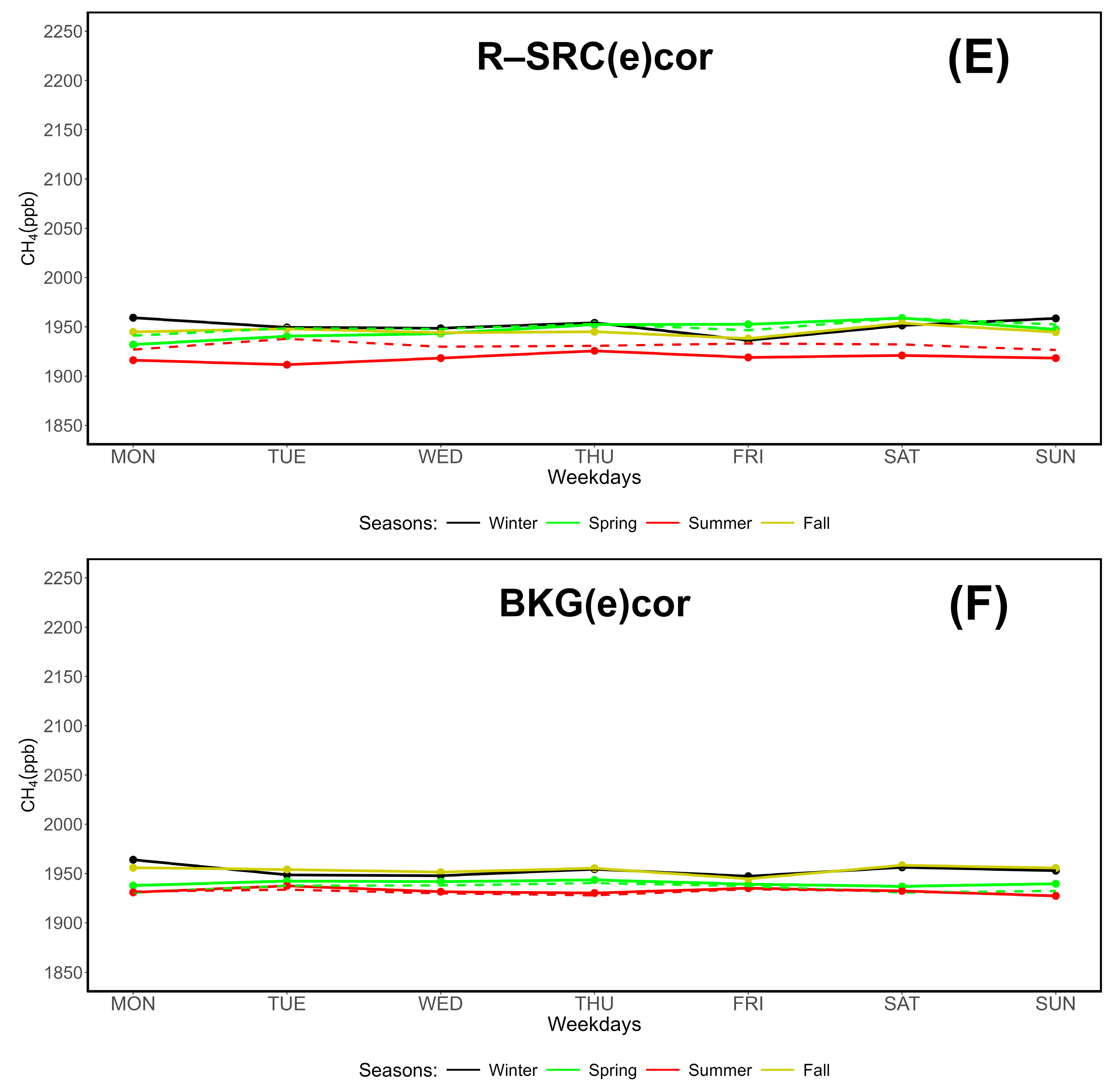
As in Section 4.2, “ecor” values data are featured in R–SRCcor (E) and BKGcor (F) plots as dashed lines.
Figure 6.
Weekly cycle (MON-SUN) of carbon monoxide (CO, ppb) under different proximity categories. A: LOC; B: N–SRC; C: R–SRC; D: BKG; E: corrected R–SRC; F: corrected BKG. Enhanced corrections (ecor) are shown as dashed lines in E and F.
Figure 6.
Weekly cycle (MON-SUN) of carbon monoxide (CO, ppb) under different proximity categories. A: LOC; B: N–SRC; C: R–SRC; D: BKG; E: corrected R–SRC; F: corrected BKG. Enhanced corrections (ecor) are shown as dashed lines in E and F.
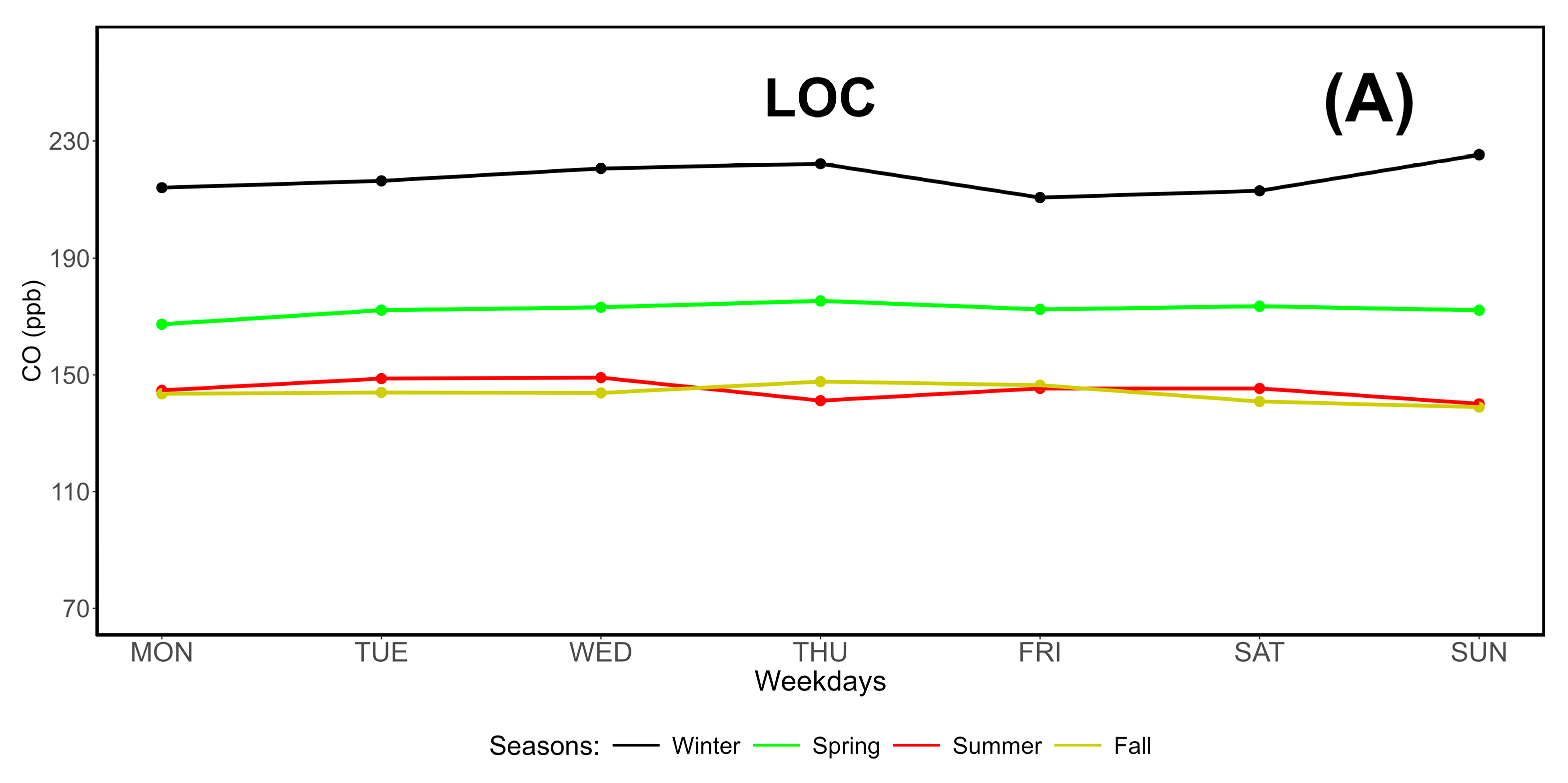
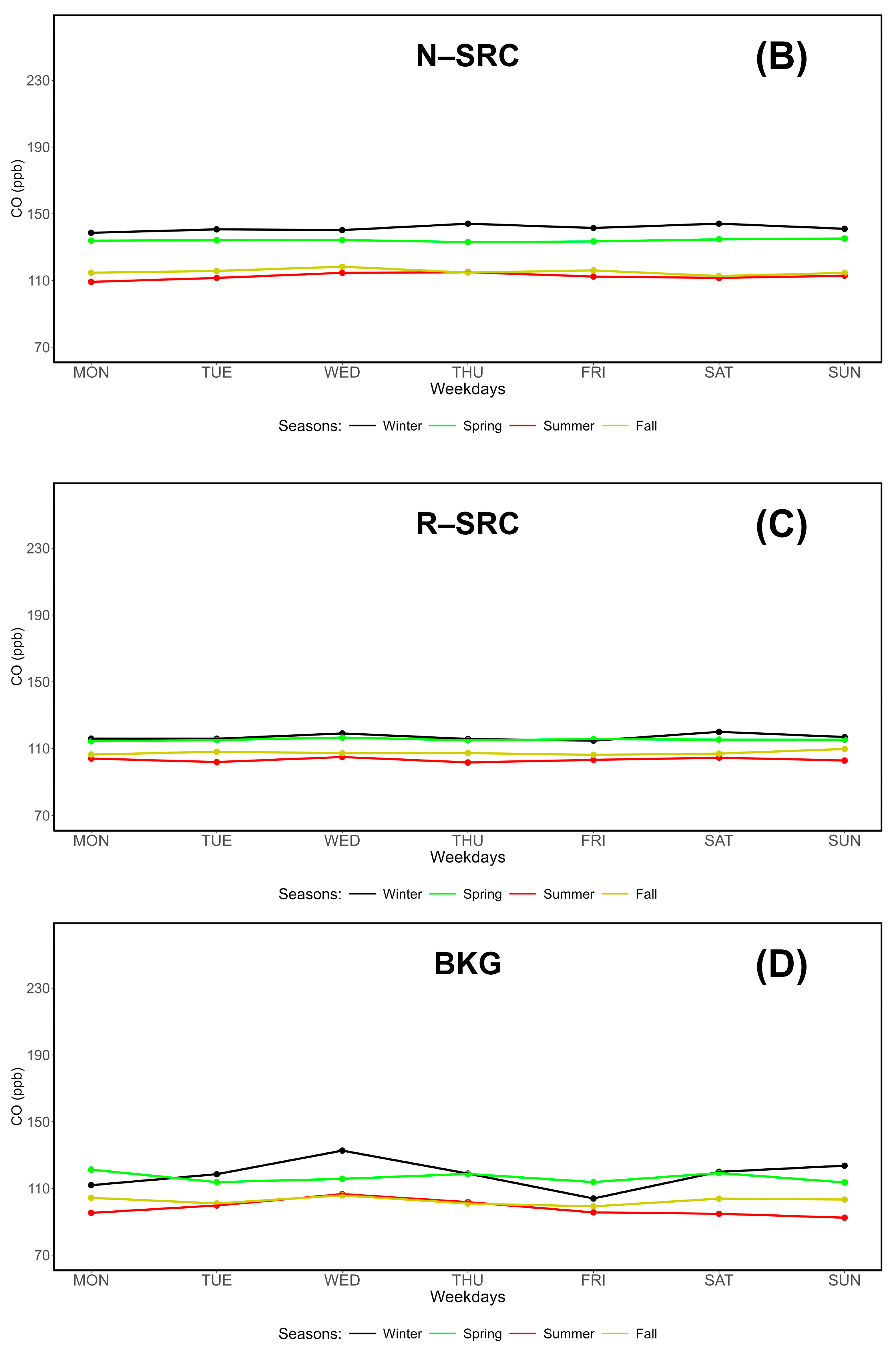
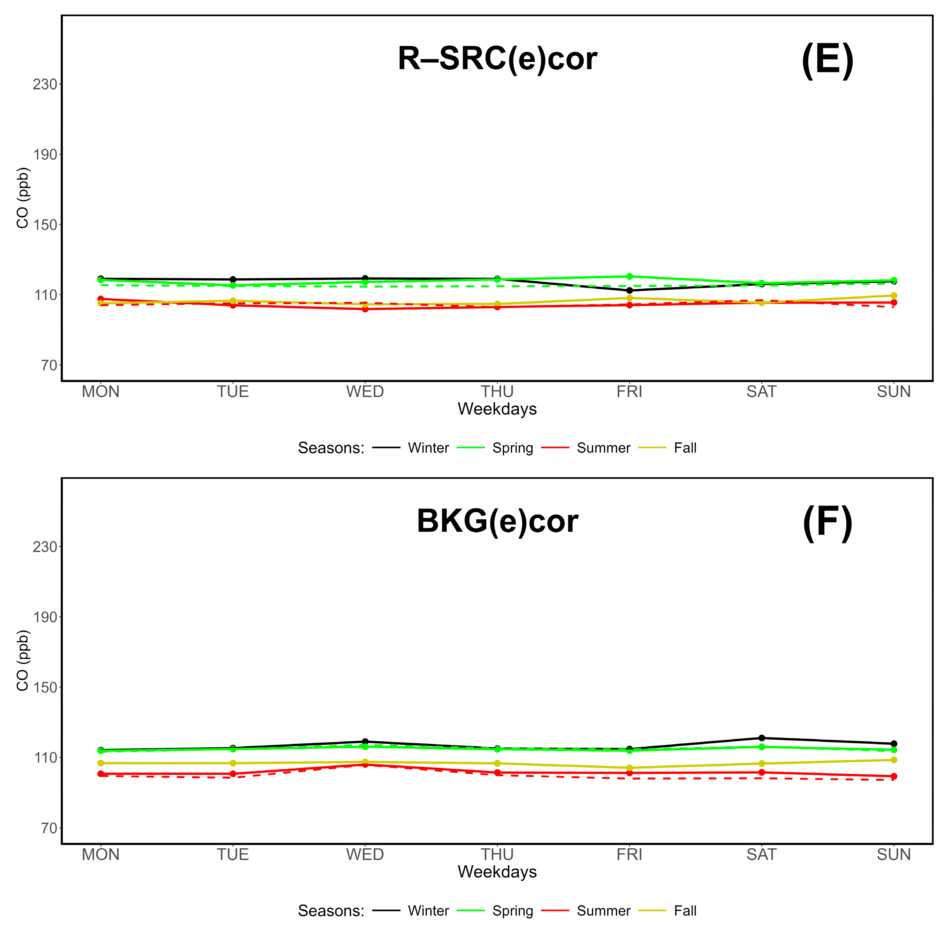
Figure 7.
Weekly cycle (MON-SUN) of carbon dioxide (CO2, ppm) under different proximity categories. A: LOC; B: N–SRC; C: R–SRC; D: BKG; E: corrected R–SRC; F: corrected BKG. Enhanced corrections (ecor) are shown as dashed lines in E and F.
Figure 7.
Weekly cycle (MON-SUN) of carbon dioxide (CO2, ppm) under different proximity categories. A: LOC; B: N–SRC; C: R–SRC; D: BKG; E: corrected R–SRC; F: corrected BKG. Enhanced corrections (ecor) are shown as dashed lines in E and F.
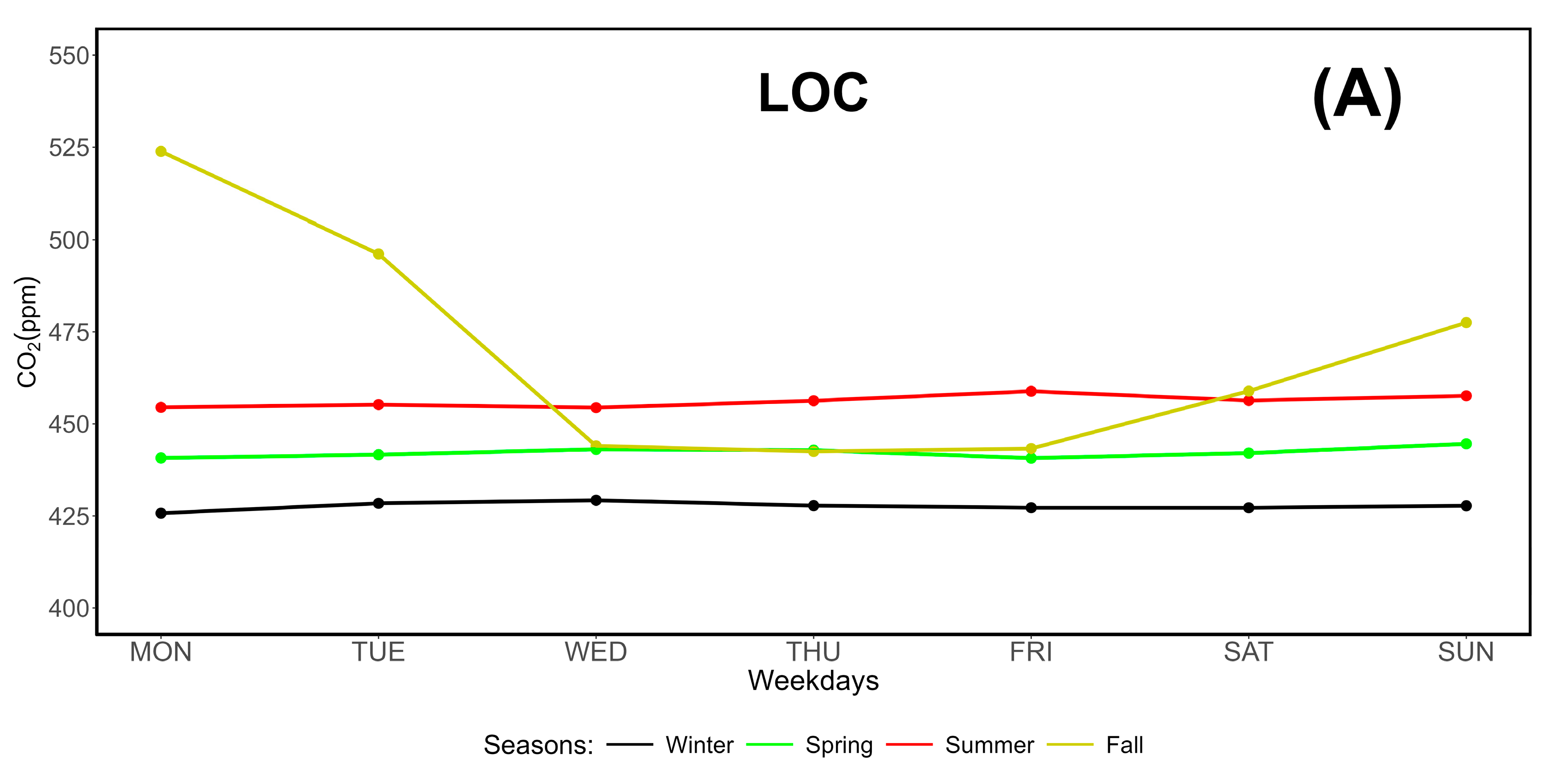
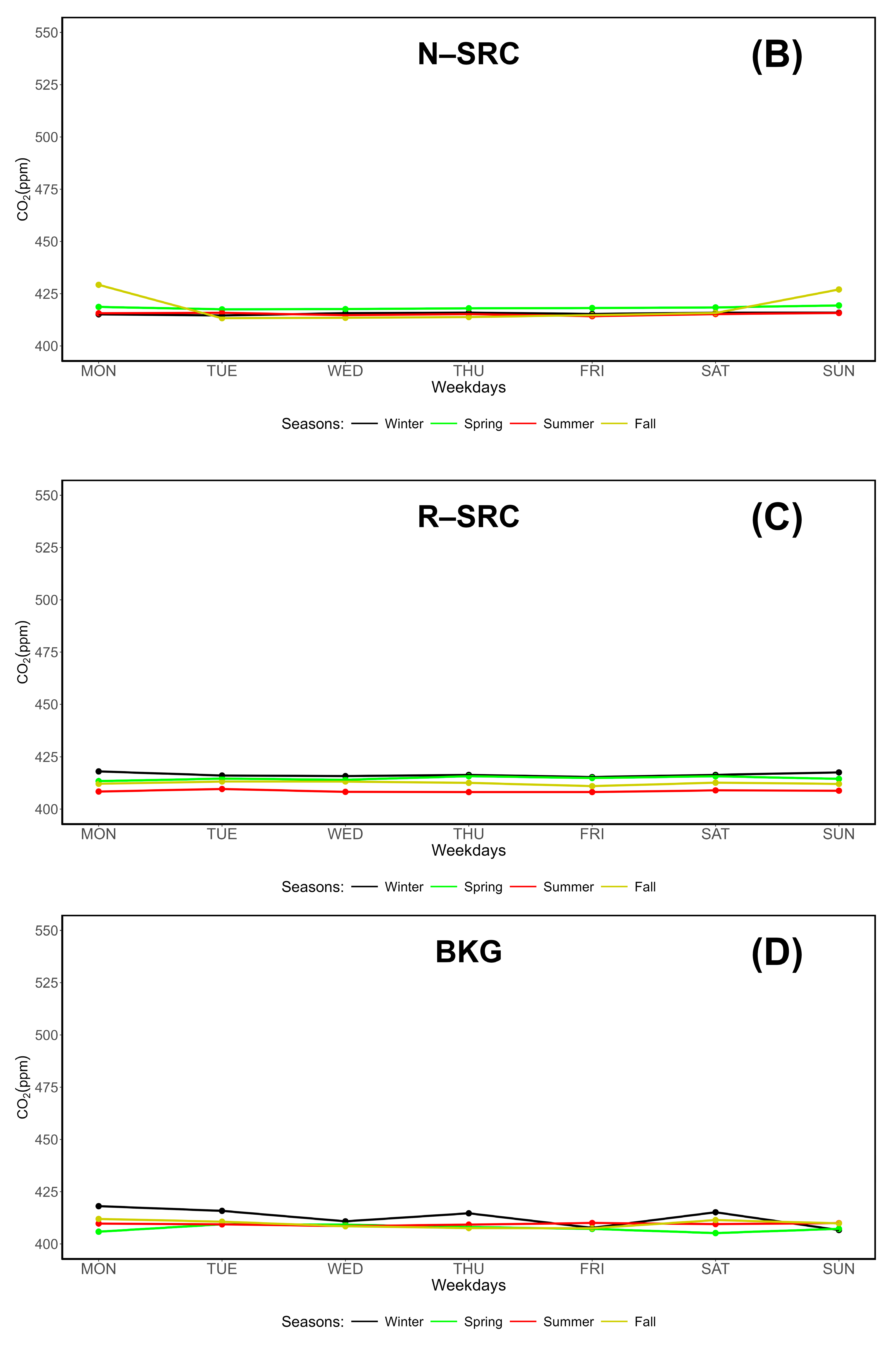
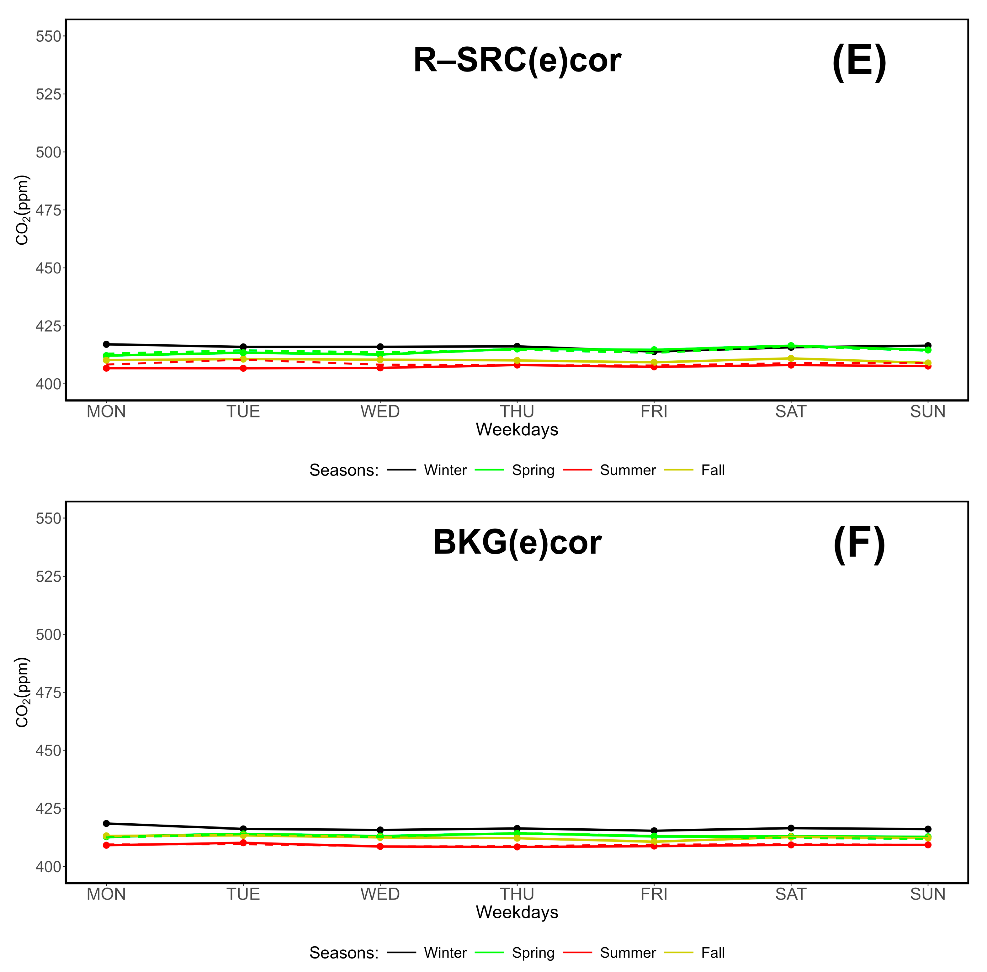
Figure 8.
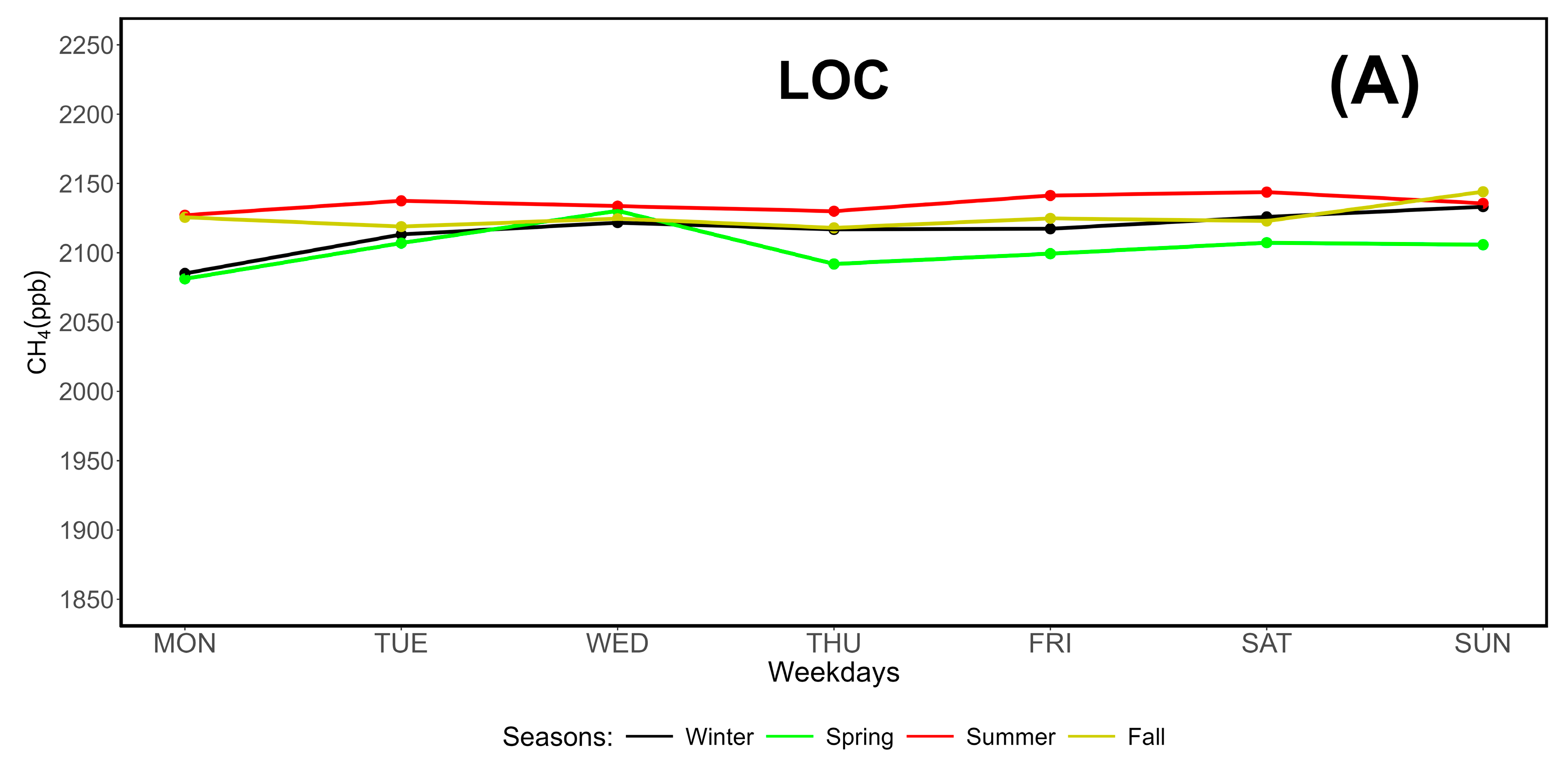
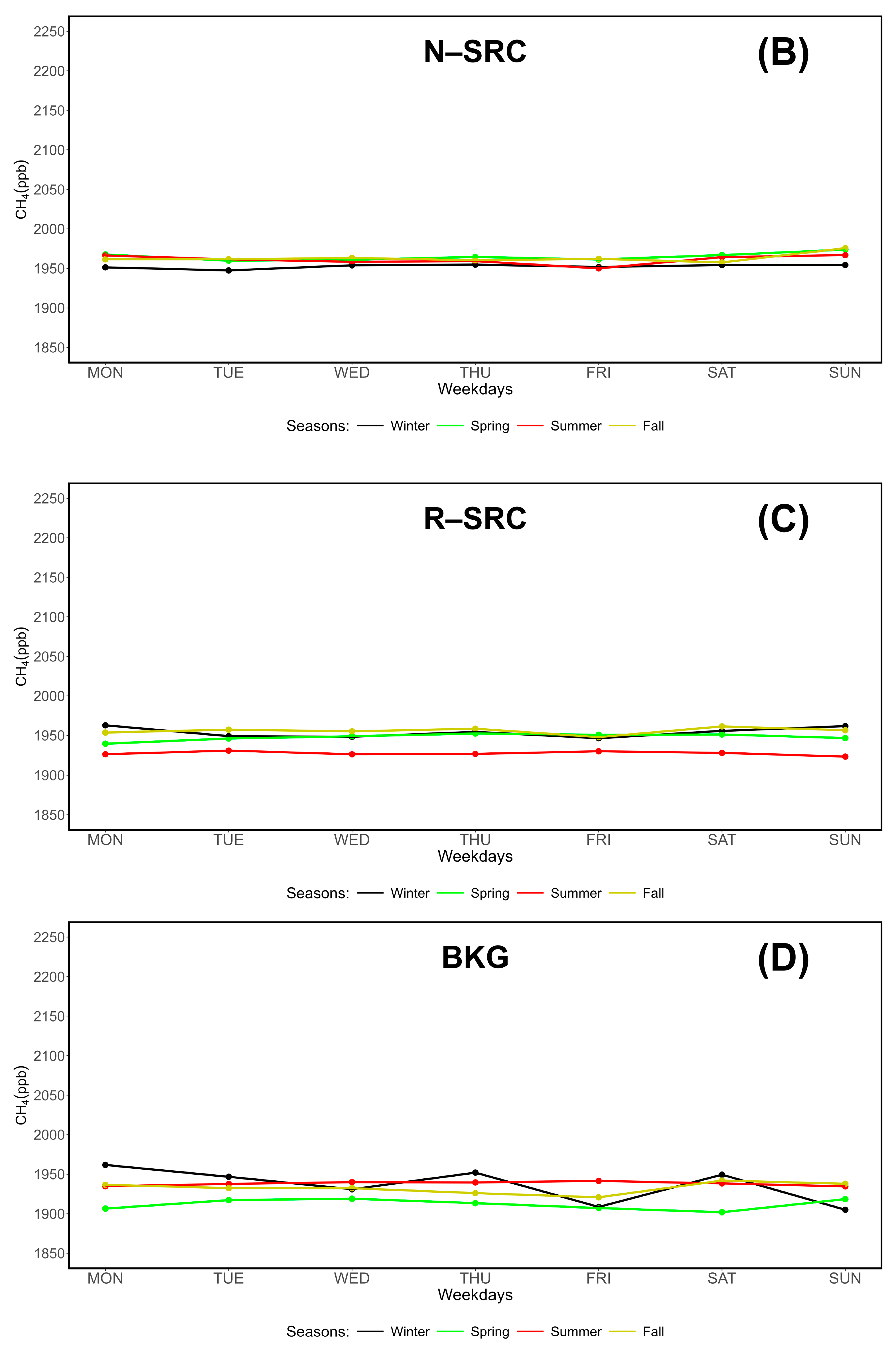
Weekly cycle (MON-SUN) of methane (CH4, ppb) under different proximity categories. A: LOC; B: N–SRC; C: R–SRC; D: BKG; E: corrected R–SRC; F: corrected BKG. Enhanced corrections (ecor) are shown as dashed lines in E and F.
Figure 8.
Weekly cycle (MON-SUN) of methane (CH4, ppb) under different proximity categories. A: LOC; B: N–SRC; C: R–SRC; D: BKG; E: corrected R–SRC; F: corrected BKG. Enhanced corrections (ecor) are shown as dashed lines in E and F.
4.4. Seasonal Variability by Wind Sector
In Section 3, wind roses showing the distribution of speeds and directions based on the main proximity categories was shown. In (carbon monoxide, ppb), (carbon dioxide, ppm), and (methane, ppb), bivariate plots show seasonal changes based on observed wind directions and speeds, without accounting for proximity categories.
Figure 9.
Seasonal variability of carbon monoxide (CO, ppb) with respect to observed wind speeds and directions during the observation period 2015-2023.
Figure 9.
Seasonal variability of carbon monoxide (CO, ppb) with respect to observed wind speeds and directions during the observation period 2015-2023.
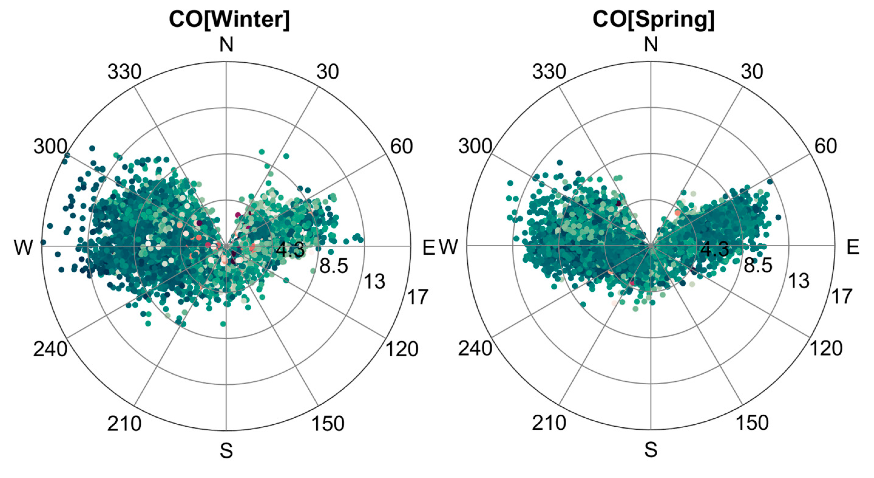

Figure 10.
Seasonal variability of carbon monoxide (CO2, ppm) with respect to observed wind speeds and directions during the observation period 2015-2023.
Figure 10.
Seasonal variability of carbon monoxide (CO2, ppm) with respect to observed wind speeds and directions during the observation period 2015-2023.
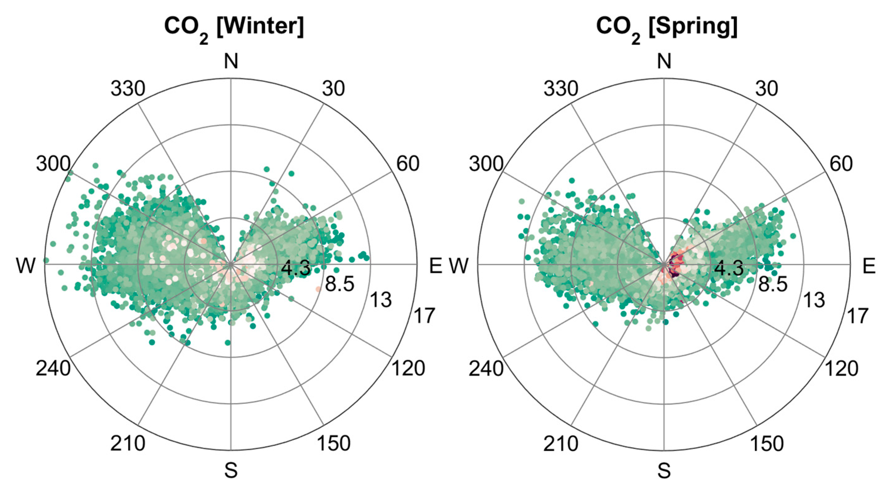
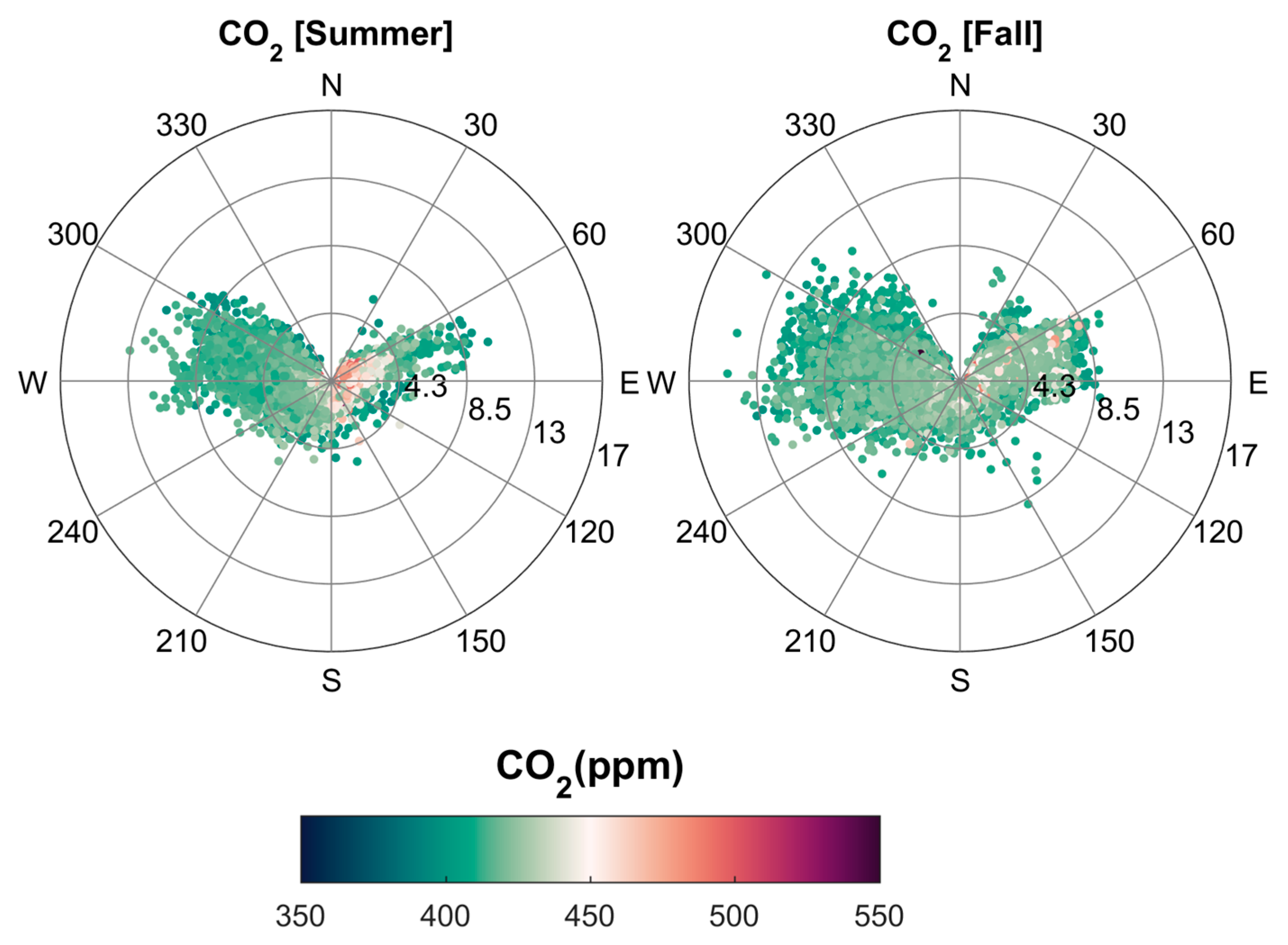
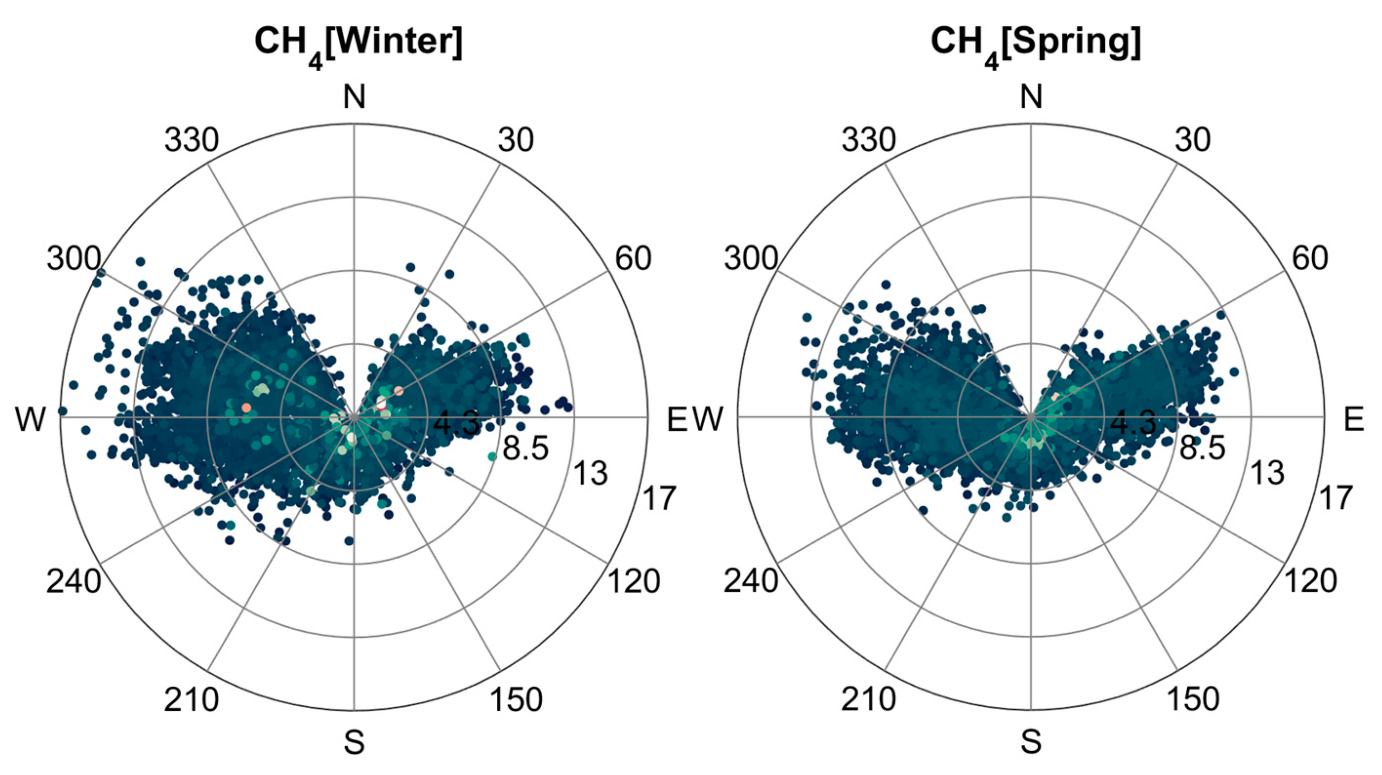
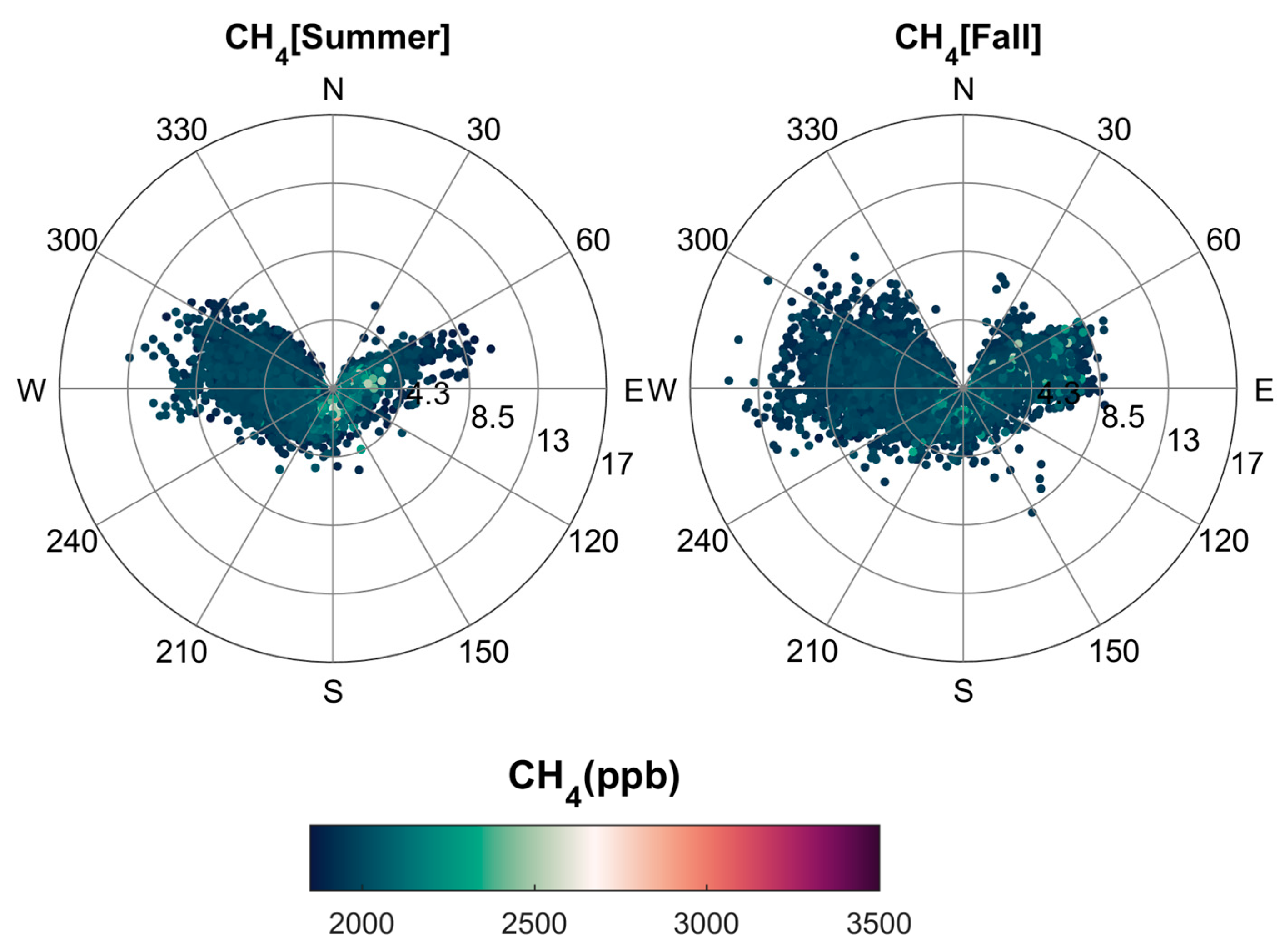
Figure 11.
Seasonal variability of carbon monoxide (CH4, ppb) with respect to observed wind speeds and directions during the observation period 2015-2023.
Figure 11.
Seasonal variability of carbon monoxide (CH4, ppb) with respect to observed wind speeds and directions during the observation period 2015-2023.
4.5. Correlations with Wind Speed by Corridors
The multi-year evaluations of methane [62] and surface ozone [61] were also based on a correlation with wind speeds based on the main corridors (western-seaside at 240–300 °N, and northeastern-continental at 0–90 °N) which are the result of local circulation. In addition to the two corridors, each representative of distinct anthropogenic influences, total data (including those falling outside the 0–90 °N and 240–300 °N wind direction ranges) were also evaluated. The analysis allowed to identify the HBP (Hyperbola Branch Pattern) of methane from the northeastern sector [62], which was not observed in surface ozone [61].
4.6. Infra- and Multi-Year Variability
As described in Section 1, the three analyzed compounds are characterized by different atmospheric lifetimes, balances between anthropogenic and natural sources, and multi-year trends. In Figure 15, monthly aggregated are used to show in greater detail the infra-annual variability based on proximity categories.
The final step of these assessments is the aggregation of data throughout the entire observation period (2015-2023), differentiated by proximity category, to verify multi-year trends. In Figure 16, monthly aggregated have been used.
5. Discussion
At the Lamezia Terme (code: LMT) WMO/GAW (World Meteorological Organization – Global Atmosphere Watch) regional station located in the southern Italian region of Calabria, an investigation based on the ratio between surface ozone and nitrogen oxides (O3/NOx) as an air mass aging and proximity indicator has allowed an unprecedented characterization of local-to-remote sources of CO, CO2, and CH4 at the site. The study is based on nine continuous years of measurements (2015-2023) and expands on the preliminary data analyzed by Cristofanelli et al. (2017) [60], which used the same method to assess the distribution of emission sources in the area.
An ideal implementation of this ratio in atmospheric research is affected by NOx measurement issues. In fact, the previous study applied a correction of NO2/2 to compensate for the overestimation of NO2 in instruments using heated molybdenum converters, following the findings of Steinbacher et al. (2007) [49] and other researchers. The challenge of measuring “true NOx” has been subject to research over time [54,55,56,57,58,59].
The use of proximity indicators based on the O3/NOx ratio is also affected by applicability limitations. For the ratio to be used, two instruments (in this case, the Thermo 42i and 49i) need to operate at the same time and provide validated data; once defined, a proximity category requires at least another instrument (e.g., Picarro G2401) to operate in conjunction with O3 and NOx data gathering, thus potentially reducing the number of data which can be evaluated. Should wind data be integrated (e.g., Vaisala WXT520), a further potential reduction of the available dataset would occur. In this study, Table 1 shows the limits of proximity categorization: Thermo 42i and 49i had a total hourly coverage (between 2015 and 2023) of 90.24% and 92.68%, respectively, however when their validated data are combined to calculate the proximity categories (LOC, N–SRC, R–SRC, BKG), the total coverage is reduced to 88.64%. The integration of Picarro G2401 data on CO, CO2, and CH4, as well as that of Vaisala WXT520 for wind data, reduced the coverage to 82.60% and 79.42%, respectively. Each instrument is characterized by high coverage rates throughout the observation period, however the G2401 has limitations in 2022 (83.89%) and 2023 (66.76%), which affect the entire dataset. The Thermo instruments have high coverage rates except for 2022 (T42i, 69%). Vaisala data have generally very high rates, however 2018 is characterized by a significant reduction (77.05%).
Reductions in the coverage rate of a specific instrument do not have a major impact on the total coverage if the gaps in the available dataset are shared between instruments: however, when the gaps do not overlap, the reduction is propagated over the final result. One example is the year 2015, which has a combined rate of 86.99% despite all instruments having rates above 90%. The results shown in Table 1 therefore indicate many ways by which total data availability could be reduced.
As a coastal site located in a central Mediterranean region (Figure 1A), LMT is subject to warm boreal summers; in addition to this, the site is affected by well-defined wind circulation patterns which are oriented on a western-northeastern axis [96,97]. These characteristics have a direct impact on the measurement of gases, aerosols and other pollutants, as western-seaside winds generally yield lower concentrations compared to northeastern-continental winds which are enriched in anthropogenic outputs [62]. This was verified in particular for methane following a multi-year (2016-2022) analysis of the compound’s behavior at LMT.
Very high O3/NOx ratios linked to westerly winds and warm seasons had already been reported in the previous study on proximity categories [60] but were not considered for an actual correction of surface ozone in the ratio used as proximity indicator. While NOx has not been subject to a detailed cyclic and multi-year analysis at LMT, ozone’s behavior has been described in detail in D’Amico et al. (2024d) [61] using nine years of data (2015-2023) which match the dataset used in this study. During warm seasons, photochemical activity influence on ozone concentrations is tangible and may lead to a further overestimation. In this study, a correction factor of O3/2 has been applied under specific conditions where the age of gathered air masses could be altered by ozone overproduction: westerly winds (240-300 °N), warm boreal seasons (March-August), diurnal measurements (10:00-16:00 UTC). The applied conditions are in accordance with the findings of works in literature which showed enhanced surface ozone formation in the presence of solar radiation and nitrogen oxides [106,107], but also consider LMT’s characteristics with respect to wind corridor orientation and previous findings on ozone patterns in the area [61].
Table 2 shows the implementation of proximity categories and their corrected versions while Table 3 compares changes in their frequency rates, i.e. whether the implementation of a given correction increases or reduces the frequency of a category. In accordance with the findings of Cristofanelli et al. (2017) [60], the frequency of data peaks at LOC/N–SRC and shows minima at BKG, with R–SRC yielding an intermediate coverage. In two (2015, 2022) out of nine years, LOC is the most common category; the remaining seven years show that N–SRC is the most represented category at LMT. BKG has the lowest rates, with three years in a row (2017-2019) yielding coverages below 1%. 2022 is also affected by a coverage slightly lower than the 1% threshold, at 0.95%. Following the implementation of the first correction (cor), BKGcor rates significantly increased and peaked at 2020 (20.7%) and 2023 (27.07%). Conversely, R–SRCcor rates dropped to the 2.33-5.06% interval. These results show the importance of assessing corrections and proximity categories over multiple years of data, as focusing on preliminary results alone does not provide accurate information on the applicability of corrections and their implications.
The ”ecor” correction introduced in this study, as shown in Table 3, systematically reduces R–SRCecor in favor of BKGecor. BKGecor has higher rates compared to R–SRCecor in all years except for 2022 (6.27% vs. 5.16%). In 2019, the two rates are nearly identical (5% vs. 5.46%). Considering that, overall, N–SRC has a higher frequency compared to LOC, BKGecor yielding higher frequency rates than R–SRCecor may not be representative of the effectiveness of the correction.
The implementation of wind speeds and direction provides a better understanding of primary corrections on the dataset. In fact, in Figure 2 LOC is linked to generally low wind speeds and a consistent contribution from the northeastern sector, which is in accordance with the findings of D’Amico et al. (2024a) [62] on the correlation between methane peaks and low wind speeds from the northeast. N–SRC is more subject to high wind exposure from the west and reduced coverage in the 30-60 °N range which is compatible with the location of downtown Lamezia Terme (Figure 1B) and various sources of anthropogenic pollution. The uncorrected R–SRC and BKG have distinct peculiarities: the former is linked to the highest wind speeds observed from the west and generally high speeds from the northeast, while the latter has a clear gap in the 30-60 °N, which effectively acts as a blind spot from a number of anthropogenic sources, moderate speeds from the westerly sector. Considering the local orography, the data lined up on the 60 °N direction for BKG may indicate winds channeled through the Marcellinara gap, possibly coming directly from the Ionian Sea with reduced anthropogenic influences in the way.
With the implementation of the primary correction, R–SRCcor shows a new blind spot in the same range described for uncorrected BKG, and generally reduces its peak westerly speeds, as well as the total amount of data from the northeast. BKGcor increases its frequency on the western sector and partially fills the previous gap of 30-60 °N.
In Cristofanelli et al. (2017) [60], it was proposed that local sources of CH4 emissions such as livestock farming were responsible for the peaks linked to the LOC category. D’Amico et al. (2024a) [62], in the analysis of seven continuous years of measurements (2016-2022), reported additional local sources of emissions, such as the A2 highway and landfills, and well-defined correlations between CH4 peaks and wind patterns. Specifically, a HBP or “Hyperbola Branch Pattern” for CH4 was observed with respect to the northeastern-continental sector, with high concentrations of CH4 linked to low wind speeds, and vice versa, low concentrations linked to high speeds. This characteristic was also observed in a study on reduced anthropogenic emissions at the time of the first 2020 COVID-19 lockdown in Italy [93].
The evaluation of the absolute concentrations of all gases based on proximity categories, shown in Table 4, provides a more detailed understanding of the balance between local and remote sources. LOC is linked to the highest peaks of all compounds, and the averaged concentrations become lower in the entire progression from LOC to BKG, with the latter being considered representative of the atmospheric background. Both types of corrected categories (cor, ecor), do not show true minima in BKG concentrations: BKG values of CO, CO2, and CH4 are systematically lower than their BKGcor and BKGecor counterparts. R–SRC categories, however, do not show a prevailing trend. These results may indicate that uncorrected BKG, which have very low frequencies at the site, may have concentrations representative of relatively unpolluted atmospheric background conditions, while BKGcor and BKGecor, with their higher frequency rates, may have retained more polluted values which increased the average. With seasons being considered, as shown in Table 5, LOC still retains the highest peaks and differences between the interplay of various sources can be noticed: for CO, the contribution of domestic heating and other forms of biomass burning lead to an absolute peak of 217.324 ± 82.18 ppb; the summer season, which is characterized by open fire emissions [105], has a lower average for LOC as well as other proximity categories. This is likely due to wildfire emissions being linked to punctual bursts in concentration during the summer, while winter concentrations constantly high throughout the entire season. In fact, the BKG minimum at 97.822 ± 22.30 ppb could be considered representative of background summertime levels characterized by the absence of wildfire-related peaks. With respect to CO2, the absolute peak is reported in LOC fall seasons, at 468.575 ± 395.02 ppm, while the winter LOC counterpart yields the lowest value for the category, at 427.627 ± 15.99 ppm. CH4 confirms the peaks observed for LOC in the study based on preliminary data [60]: however, the seasonal variability in LOC is not in accordance with the general variability observed in D’Amico et al. (2024a) [62] which linked CH4 peaks to the winter season. In fact, LOC CH4 concentrations peak at summer (2135.630 ± 176.26 ppb) and fall (2125.003 ± 165.83 ppb), and in the case of N–SRC, winter has the lowest concentration of the category at 1952.578 ± 42.87 ppb compared to the spring peak of 1964.990 ± 66.35 ppb. If agriculture, manure, and livestock are indeed responsible for LOC peaks at LMT, one possibility would be changes in the CH4 outputs of livestock and agricultural sources based on seasonal changes, such as different diets [108,109,110,111].
The evaluation of the daily cycle, which is one of LMT’s peculiarities due to local wind circulation and the behavior of aerosols and gases at the site [15,61,62,93]. As seen in Figs. 3 (CO), 4 (CO2), and 5 (CH4), the “proper” daily cycle as defined in previous research is limited to the LOC categories, while the other categories (especially R–SRC and BKG) show flat patterns and a general progression from LOC peaks to BKG minima. CO and CO2 were not subject to detailed multi-year and cyclic analyses, therefore CH4 is more representative of the differences reported between general variability (also accounting for seasons) and proximity-category dependent variability. CO’s LOC (Figure 3A) shows seasonal trends in accordance with the other findings, as the winter concentrations dominate and report night-time peaks compatible with domestic heating, while the summer is characterized by a flat pattern, compatible with sporadic bursts linked to biomass burning. CO2 shows a well-defined fall anomaly in LOC (Figure 4A) and N–SRC (Figure 4B), as already shown by the findings described above. The LOC daily cycle of CH4 shown in Figure 5A is similar to the uncategorized cycle described in D’Amico et al. (2024a) [62]. The N–SRC behavior seen in Figure 5B shows a similar trend, characterized by heavy smoothing and a flat pattern. These findings also prove the importance of proximity categorization, which in this case has allowed to discriminate totally different daily cycles which were not observed before at LMT.
The observation site of LMT served as a proving ground in the Italian peninsula for weekly analyses [61,62,63]. The weekly cycle has been assessed in a number of studies under the assumption that no natural phenomenon would discriminate between weekdays (MON-SUN), while anthropic activities do change during the course of a standard week and may do so with seasonal differences [63]. In this evaluation, it was initially assumed that the LOC and N–SRC categories would show well define differences between MON-FRI (weekdays latu sensu) and SAT-SUN (weekends); due to the proximity to anthropogenic sources, weekly patterns should be noticeable, while R–SRC and BKG would combine various outputs over longer time scales, thus “hiding” the weekly cycle. Contrary to expectations, despite differences being reported in absolute concentrations between LOC and BKG in Figs. 6 (CO), 7 (CO2), and 8 (CH4), no relevant weekly cycle was observed. The only evidence of a weekly trend are reported for CO2 in LOC (Figure 7A) and, at a lower rate, in N–SRC (Figure 7B), and they are both limited to fall concentrations. The nature of these CO2 anomalies during the fall season require additional investigation. The absence of a LOC weekly cycle would be explained, in the case of CH4, by emissions from the agricultural sector (livestock included), which are not expected to change during the course of a standard week. LOC CO and CO2 may be explained by a balance between industrial and transportation-related emissions during MON-FRI, and domestic emissions during SAT-SUN. These hypotheses require further investigation in future studies accounting for additional atmospheric tracers. As shown in Figs. 9 (CO), 10 (CO2), and 11 (CH4), the interplay between wind direction, speeds, and gas concentrations at LMT is dependent on local circulation, so a number of anthropogenic and natural sources other than the ones mentioned in this study (Figure 1B) could be considered. By analyzing wind corridors and related speeds, some of the hypotheses raised in previous works can be validated: in Figs. 12 (CO), 13 (CO2), and 14 (CH4), the HBP (Hyperbola Branch Pattern) hypothesis first assumed in D’Amico et al. (2024a) [62] is now validated by chemical data. In fact, the pattern and the influence of anthropogenic emissions linked to low wind speeds were first assumed based on the “exposure” of ambient air to anthropogenic pollution: with low wind speeds, ambient air from the northeastern sector is enriched in pollutants, while high speeds do not have the time to trigger the same effect. This hypothesis is now corroborated by the O3/NOx ratio, hence by a chemical factor in addition to a physical one, as the LOC observations in in Figs. 12 (CO), 13 (CO2), and 14 (CH4) do show concentration peaks at low speeds, in accordance with the hypothesis.
This research concludes with the infra-annual (Figure 15) and multi-year (Figure 16) analyses of the three gases. Monthly aggregations allow to define infra-annual variability with greater detail, and a clear difference between LOC and other categories shown for all gases. CO2 is characterized by a median (summer) peak which does not match the general trend of this compound, as summer concentrations are generally lower due to photosynthesis activity [112]. However, many pollutants can interfere with the photosynthesis process and therefore reduce CO2 uptake by the biosphere [113]. The local behavior of CO2 would then require further investigation via the implementation of additional atmospheric tracers capable of differentiating between natural and anthropogenic sources. Figure 16 show a multi-year variability in accordance with general trends as described in Section 1: CO2 and CH4 are increasing globally, as confirmed at LMT by R–SRC and BKG variability between 2015 and 2023, while LOC concentrations are more susceptible to local sources. CO shows major fluctuations which are not linked to a well-defined increase or decrease, however the influence of wildfire emissions [72,73] and fossil fuel emission mitigation strategies and policies [70,71] can impact the variability seen for BKG and R–SRC values at LMT.
Overall, this study has provided an unprecedented level of detail on the balance between local and remote sources of emissions at LMT, a site characterized by many peculiarities. The findings of this study with respect to the atmospheric background levels seen in Figure 16 could be integrated by other measurements, such as the deviations from the VPDB (Vienna Pee Dee Belemnite) standard [114] of the carbon-13 to carbon-12 ratio (13C/12C) in CH4 (δ13C-CH4) and CO2 (δ13C-CO2), which is an effective tracer of anthropogenic and natural emissions [112,115,116,117]. The LMT observation site is part of the developing cross country network of continuous carbon isotope measurements, together with Lampedusa (LMP) in the Strait of Sicily, Potenza (POT) in the neighboring region of Basilicata, and Mt. Cimone (CMN) in the northern region of Emilia-Romagna [118]. The implementation of proximity indicators could differentiate background levels of δ13C-CH4 and δ13C-CO2 from those affected by anthropogenic emissions, and vice versa, characteristic isotopic fingerprints representative of the atmospheric background could be used to validate indicators based on the O3/NOx ratio and their respective corrections, including the “enhanced correction” (ecor) introduced in this study. Future research based on these integrated methodologies could therefore increase the accuracy of atmospheric measurements aimed at background and unpolluted levels and define the applicability of corrections to other stations across the globe.
6. Conclusions
At the Lamezia Terme (LMT) WMO/GAW (World Meteorological Organization – Global Atmosphere Watch) observation site in Calabria, Southern Italy the ratio between surface ozone and nitrogen oxides (O3/NOx) has been used as a proximity indicator to assess, with unprecedented detail for the site, the source attribution between LOC (local), N–SRC (near source), R–SRC (remote source), and BKG (background) concentrations of carbon monoxide (CO), carbon dioxide (CO2), and methane (CH4). The study expands on the findings of previous research based on preliminary data gathered at the site by using nine full years (2015-2023) of observations.
The implementation of these methodologies is faced by numerous challenges, such as measurement coverage rates and the possible overestimation of NO2 by certain instruments. The previous work used a correction factor on NO2, which is also applied and expanded in this research; furthermore, this study introduces a new correction factor for ozone, based on the cyclic and multi-year assessment of this compound at the LMT site.
The results of the study confirm a number of hypotheses raised in previous works on the peaks observed at the site: methane peaks are attributed to the LOC category, indicating local sources of emission such as agriculture and livestock farming; local emissions with increased concentrations of CO, CO2, and CH4 are linked to low wind speeds from the northeastern sector, which is subject to anthropogenic pollution; seasonal variabilities show changes in the nature of sources of emission (e.g., summertime open fires and wintertime biomass burning). In addition to the findings and the validation of hypotheses raised in previous works, a number of observations such as weekly trends and the interplay of local anthropogenic and natural sources have not shown the expected differentiation. Furthermore, the behavior of CO2 under specific conditions raises questions with respect with the balances of emissions and sinks in the area. These discrepancies require further investigations and the implementation of additional atmospheric tracers, such as carbon isotope ratios in CO2 and CH4.
The study also underlines the importance of performing ad hoc corrections to the measurements performed at a given observation site, accounting for the site’s characteristic wind circulation patterns, climate, and variability in the concentrations of atmospheric gases. The same corrections could be applied to atmospheric observation sites showing similar characteristics.
Author Contributions
Conceptualization, F.D.; methodology, F.D. and T.L.F.; software, F.D. and T.L.F.; validation, T.L.F., D.G., I.A., S.S., G.D.B. and C.R.C.; formal analysis, F.D. and T.L.F.; investigation, F.D.; data curation, F.D., T.L.F., D.G., I.A., L.M., S.S., G.D.B. and C.R.C.; writing—original draft preparation, F.D.; writing—review and editing, F.D., T.L.F., D.G., I.A., M.D.P., L.M., S.S., G.D.B. and C.R.C.; visualization, F.D. and T.L.F.; supervision, C.R.C.; funding acquisition, M.D.P. and C.R.C. All authors have read and agreed to the published version of the manuscript.
Funding
This research was funded by AIR0000032 – ITINERIS, the Italian Integrated Environmental Research Infrastructures System (D.D. n. 130/2022 - CUP B53C22002150006) under the EU - Next Generation EU PNRR - Mission 4 “Education and Research” - Component 2: “From research to business” - Investment 3.1: “Fund for the realization of an integrated system of research and innovation infrastructures”.
Institutional Review Board Statement
Not applicable.
Informed Consent Statement
Not applicable.
Data Availability Statement
The datasets presented in this article are not readily available because they are part of other ongoing studies.
Acknowledgments
TBFIL.
Conflicts of Interest
The authors declare no conflicts of interest.
References
- Stevens, R.K.; Dzubay, T.G.; Lewis, C.W.; Shaw, R.W., Jr. Source apportionment methods applied to the determination of the origin of ambient aerosols that affect visibility in forested areas. Atmos. Environ. 1984, 18, 261–272. [Google Scholar] [CrossRef]
- Shah, J.J.; Kneip, T.J.; Daisey, J.M. Source apportionment of carbonaceous aerosol in New York City by multiple linear regression. J. Air Pollut. Control Assoc. 1985, 35, 541–544. [Google Scholar] [CrossRef]
- Khalil, M.A.K.; Rasmussen, R.A. Carbon monoxide in an urban environment: application of a receptor model for source apportionment. J. Air Pollut. Control Assoc. 1988, 38, 901–906. [Google Scholar] [CrossRef]
- Wolff, G.T.; Korsog, P.E. Atmospheric concentrations and regional source apportionments of sulfate, nitrate and sulfur dioxide in the Berkshire mountains in western Massachusetts. Atmos. Environ. 1989, 23, 55–65. [Google Scholar] [CrossRef]
- Nisbet, E.G.; Fisher, R.E.; Lowry, D.; France, J.L.; Allen, G.; Bakkaloglu, S.; Broderick, T.J.; Cain, M.; Coleman, M.; Fernandez, J.; et al. Methane Mitigation: Methods to Reduce Emissions, on the Path to the Paris Agreement. Rev. Geophys. 2020, 58, e2019RG000675. [Google Scholar] [CrossRef]
- Zazzeri, G.; Graven, H.; Xu, X.; Saboya, E.; Blyth, L.; Manning, A.J.; Chawner, H.; Wu, D.; Hammer, S. Radiocarbon Measurements Reveal Underestimated Fossil CH4 and CO2 Emissions in London. Geophys. Res. Lett. 2023, 50, e2023GL103834. [Google Scholar] [CrossRef]
- Ducruet, C.; Polo Martin, B.; Sene, M.A.; Lo Prete, M.; Sun, L.; Itoh, H.; Pigné, Y. Ports and their influence on local air pollution and public health: A global analysis. Sci. Total Environ. 2024, 915, 170099. [Google Scholar] [CrossRef]
- Siciliano, T.; De Donno, A.; Serio, F.; Genga, A. Source Apportionment of PM10 as a Tool for Environmental Sustainability in Three School Districts of Lecce (Apulia). Sustainability 2024, 16, 1978. [Google Scholar] [CrossRef]
- Jordanov, D.L.; Dzolov, G.D.; Sirakov, D.E. Effect of planetary boundary layer on long-range transport and diffusion of pollutants. C. R. Acad. Bulg. Sci. 1979, 32, 1635–1637. [Google Scholar]
- McNider, R.T.; Moran, M.D.; Pielke, R.A. Influence of diurnal and inertial boundary-layer oscillations on long-range dispersion. Atmos. Environ. 1988, 22, 2445–2462. [Google Scholar] [CrossRef]
- Zhao, D.; Tie, X.; Gao, Y.; Zhang, Q.; Tian, H.; Bi, K.; Jin, Y.; Chen, P. In-Situ Aircraft Measurements of the Vertical Distribution of Black Carbon in the Lower Troposphere of Beijing, China, in the Spring and Summer Time. Atmosphere 2015, 6, 713–731. [Google Scholar] [CrossRef]
- Farah, A.; Freney, E.; Chauvigné, A.; Baray, J.-L.; Rose, C.; Picard, D.; Colomb, A.; Hadad, D.; Abboud, M.; Farah, W.; Sellegri, K. Seasonal Variation of Aerosol Size Distribution Data at the Puy de Dôme Station with Emphasis on the Boundary Layer/Free Troposphere Segregation. Atmosphere 2018, 9, 244. [Google Scholar] [CrossRef]
- Raptis, I.-P.; Kazadzis, S.; Amiridis, V.; Gkikas, A.; Gerasopoulos, E.; Mihalopoulos, N. A Decade of Aerosol Optical Properties Measurements over Athens, Greece. Atmosphere 2020, 11, 154. [Google Scholar] [CrossRef]
- Zhou, Q.; Cheng, L.; Zhang, Y.; Wang, Z.; Yang, S. Relationships between Springtime PM2.5, PM10, and O3 Pollution and the Boundary Layer Structure in Beijing, China. Sustainability 2022, 14, 9041. [Google Scholar] [CrossRef]
- D’Amico, F.; Calidonna, C.R.; Ammoscato, I.; Gullì, D.; Malacaria, L.; Sinopoli, S.; De Benedetto, G.; Lo Feudo, T. Peplospheric influences on local greenhouse gas and aerosol variability at the Lamezia Terme WMO/GAW regional station in Calabria, Southern Italy: a multiparameter investigation. Sustainability 2024, 16, 10175. [Google Scholar] [CrossRef]
- Tov, D.A.S.; Peleg, M.; Matveev, V.; Mahrer, Y.; Seter, I.; Luria, M. Recirculation of polluted air masses over the East Mediterranean coast. Atmos. Environ. 1997, 31, 1441–1448. [Google Scholar] [CrossRef]
- Furutani, H.; Dall’osto, M.; Roberts, G.C.; Prather, K.A. Assessment of the relative importance of atmospheric aging on CCN activity derived from field observations. Atmos. Environ. 2008, 42, 3130–3142. [Google Scholar] [CrossRef]
- Espina-Martin, P.; Perdrix, E.; Alleman, L.Y.; Coddeville, P. Origins of the seasonal variability of PM2.5 sources in a rural site in Northern France. Atmos. Environ. 2024, 333, 120660. [Google Scholar] [CrossRef]
- Parrish, D.D.; Allen, D.T.; Bates, T.S.; Estes, M.; Fehsenfeld, F.C.; Feingold, G.; Ferrare, R.; Hardesty, R.M.; Meagher, J.F.; Nielsen-Gammon, J.W.; et al. Overview of the Second Texas Air Quality Study (TexAQS II) and the Gulf of Mexico Atmospheric Composition and Climate Study (GoMACCS). J. Geophys. Res. Atmos. 2009, 114. [Google Scholar] [CrossRef]
- Morgan, W.T.; Allan, J.D.; Bower, K.N.; Highwood, E.J.; Liu, D.; McMeeking, G.R.; Northway, M.J.; Williams, P.I.; Krejci, R.; Coe, H. Airborne measurements of the spatial distribution of aerosol chemical composition across Europe and evolution of the organic fraction. Atmos. Chem. Phys. 2010, 10, 4065–4083. [Google Scholar] [CrossRef]
- Penner, J.E.; Atherton, C.S.; Dignon, J.; Ghan, S.J.; Walton, J.J.; Hameed, S. Tropospheric nitrogen—A 3-dimensional study of sources, distributions, and deposition. J. Geophys. Res. - Atmos. 1991, 96, 959–990. [Google Scholar] [CrossRef]
- Trainer, M.; Parrish, D.D.; Buhr, M.P.; Norton, R.B.; Fehsenfeld, F.C.; Anlauf, K.G.; Bottenheim, J.W.; Tang, Y.Z.; Wiebe, H.A.; Roberts, J.M.; et al. Correlation of ozone with NOy in photochemically aged air. J. Geophys. Res. – Atmos. 1993, 98, 2917–2925. [Google Scholar] [CrossRef]
- Jacob, D.J.; Heikes, E.G.; Fan, S.-M.; Logan, J.A.; Mauzerall, D.L.; Bradshaw, J.D.; Singh, H.B.; Gregory, G.L.; Talbot, R.W.; Blake, D.R.; Sachse, G.W. Origin of ozone and NOx in the tropical troposphere: A photochemical analysis of aircraft observations over the South Atlantic basin. J. Geophys. Res. - Atmos. 1996, 101, 24235–24250. [Google Scholar] [CrossRef]
- Hauglustaine, D.A.; Emmons, L.K.; Newchurch, M.; Brasseur, G.P.; Takao, T.; Matsubara, K.; Johnson, J.; Ridley, B.; Stith, J.; Dye, J. On the role of lightning NOx in the formation of tropospheric ozone plumes: A global model perspective. J. Atmos. Chem. 2001, 38, 277–294. [Google Scholar] [CrossRef]
- Henne, S.; Dommen, J.; Neininger, B.; Reimann, S.; Staehelin, J.; Prévôt, A.S.H. Influence of mountain venting in the Alps on the ozone chemistry of the lower free troposphere and the European pollution export. J. Geophys. Res. 2005, 110(D22), 307. [Google Scholar] [CrossRef]
- Stein, A.F.; Mantilla, E.; Millán, M.M. Using measured and modeled indicators to assess ozone-NOx-VOC sensitivity in a western Mediterranean coastal environment. Atmos. Environ. 2005, 39, 7167–7180. [Google Scholar] [CrossRef]
- Lee, J.D.; Moller, S.J.; Read, K.A.; Lewis, A.C.; Mendes, L.; Carpenter, L.J. Year-round measurements of nitrogen oxides and ozone in the tropical North Atlantic marine boundary layer. J. Geophys. Res. – Atmos. 2009, 114, 302. [Google Scholar] [CrossRef]
- Mavroidis, I.; Chaloulakou, A. Long-term trends of primary and secondary NO2 production in the Athens area. Variation of the NO2/NOx ratio. Atmos. Environ. 2011, 45, 6872–6879. [Google Scholar] [CrossRef]
- Fenger, J. Urban air quality. Atmos. Environ. 1999, 33, 4877–4900. [Google Scholar] [CrossRef]
- Jacob, D.J. Introduction to Atmospheric Chemistry; Princeton University Press: Princeton, NJ, USA, 1999. [Google Scholar]
- Colvile, R.N.; Hutchinson, E.J.; Mindell, J.S.; Warren, R.F. The transport sector as a source of air pollution. Atmos. Environ. 2001, 35, 1537–1565. [Google Scholar] [CrossRef]
- Seinfeld, J.H.; Pandis, S.N. Atmospheric Chemistry and Physics; A Wiley-Inter Science Publication, John Wiley & Sons Inc.: Hoboken, NJ, USA, 2006. [Google Scholar]
- Beevers, S.D.; Westmoreland, E.; de Jong, M.C.; Williams, M.L.; Carslaw, D.C. Trends in NOx and NO2 emissions from road traffic in Great Britain. Atmos. Environ. 2012, 54, 107–116. [Google Scholar] [CrossRef]
- Liu, F.; Beirle, S.; Zhang, Q.; Dörner, S.; He, K.; Wagner, T. NOx lifetimes and emissions of cities and power plants in polluted background estimated by satellite observations. Atmos. Chem. Phys. 2016, 16, 5283–5298. [Google Scholar] [CrossRef]
- Staehelin, J.; Thudium, J.; Buheler, R.; Volz-Thomas, A.; Graber, W. Trends in surface ozone concentrations at Arosa (Switzerland). Atmos. Environ. 1994, 28, 75–78. [Google Scholar] [CrossRef]
- Smyshlyaev, S.P.; Galin, V.Y.; Blakitnaya, P.A.; Jakovlev, A.R. Numerical Modeling of the Natural and Manmade Factors Influencing Past and Current Changes in Polar, Mid-Latitude and Tropical Ozone. Atmosphere 2020, 11, 76. [Google Scholar] [CrossRef]
- Solomon, S. Stratospheric ozone depletion: A review of concepts and history. Rev. Geophys. 1999, 37, 275–316. [Google Scholar] [CrossRef]
- Andersen, S.B.; Weatherhead, E.C.; Stevermer, A.; Austin, J.; Brühl, C.; Fleming, E.L.; De Grandpré, J.; Grewe, V.; Isaksen, I.; Pitari, G.; et al. Comparison of recent modeled and observed trends in total column ozone. J. Geophys. Res. - Atmos. 2006, 111, 4428. [Google Scholar] [CrossRef]
- Egorova, T.; Rozanov, E.; Arsenovic, P.; Sukhodolov, T. Ozone Layer Evolution in the Early 20th Century. Atmosphere 2020, 11, 169. [Google Scholar] [CrossRef]
- Palli, D.; Sera, F.; Giovannelli, L.; Masala, G.; Grechi, D.; Bendinelli, B.; Caini, S.; Dolara, P. Environmental ozone exposure and oxidative DNA damage in adult residents in Florence, Italy. Environ. Pollut. 2009, 157, 1521–1525. [Google Scholar] [CrossRef]
- Nuvolone, D.; Petri, D.; Voller, F. The effects of ozone on human health. Environ. Sci. Pollut. Res. Int. 2018, 25, 8074–8088. [Google Scholar] [CrossRef]
- Malashock, D.A.; DeLang, M.N.; Becker, J.S.; Serre, M.L.; West, J.J.; Chang, K.-L.; Cooper, O.R.; Anenberg, S.C. Estimates of ozone concentrations and attributable mortality in urban, peri-urban and rural areas worldwide in 2019. Environ. Res. Lett. 2022, 17, 054023. [Google Scholar] [CrossRef]
- Olstrup, H.; Åström, C.; Orru, H. Daily Mortality in Different Age Groups Associated with Exposure to Particles, Nitrogen Dioxide and Ozone in Two Northern European Capitals: Stockholm and Tallinn. Environments 2022, 9, 83. [Google Scholar] [CrossRef]
- Donzelli, G.; Suarez-Varela, M.M. Tropospheric Ozone: A Critical Review of the Literature on Emissions, Exposure, and Health Effects. Atmosphere 2024, 15, 779. [Google Scholar] [CrossRef]
- Dunlea, E.J. , Herndon, S.C.; Nelson, D.D.; Volkamer, R.M.; San Martini, F.; Sheehy, P.M.; Zahniser, M.S.; Shorter, J.H.; Wormhoudt, J.C.; Lamb, B.K.; et al. Evaluation of nitrogen dioxide chemiluminescence monitors in a polluted urban environment. Atmos. Chem. Phys. 2007, 7, 2691–2704. [Google Scholar] [CrossRef]
- Carvalho, V.S.B.; Freitas, E.D.; Martins, L.D.; Martins, J.A.; Mazzoli, C.R.; de Fátima Andrade, M. Air quality status and trends over the Metropolitan Area of São Paulo, Brazil as a result of emission control policies. Environ. Sci. Policy 2015, 47, 68–79. [Google Scholar] [CrossRef]
- Rivera, N.M. Air quality warnings and temporary driving bans: Evidence from air pollution, car trips, and mass-transit ridership in Santiago. J. Environ. Econ. Manag. 2021, 108, 102454. [Google Scholar] [CrossRef]
- Akintomide Ajayi, S.; Anum Adam, C.; Dumedah, G.; Adebanji, A.; Ackaah, W. The impact of traffic mobility measures on vehicle emissions for heterogeneous traffic in Lagos City. Sci. Afr. 2023, 21, e01822. [Google Scholar] [CrossRef]
- Steinbacher, M.; Zellweger, C.; Schwarzenbach, B.; Bugmann, S.; Buchmann, B.; Ordóñez, C.; Prévôt, A.S.H.; Hueglin, C. Nitrogen oxide measurements at rural sites in Switzerland: Bias of conventional measurement techniques. J. Geophys. Res. Atmos. 2007, 112. [Google Scholar] [CrossRef]
- Winer, A.M.; Peters, J.W.; Smith, J.P.; Pitts, J.N. Jr. Response of commercial chemiluminescence NO–NO2 analyzers to other nitrogen-containing compounds. Environ. Sci. Technol. 1974, 8, 1118–1121. [Google Scholar] [CrossRef]
- Grosjean, D.; Harrison, J. Response of chemiluminescence NOx analyzers and ultraviolet ozone analyzers to organic air pollutants. Environ. Sci. Technol. 1985, 19, 862–865. [Google Scholar] [CrossRef]
- Gehrig, R.; Baumann, R. Comparison of 4 different types of commercially available monitors for nitrogen oxides with test gas mixtures of NH3, HNO3, PAN and VOC and in ambient air, paper presented at EMEP Workshop on Measurements of Nitrogen-Containing Compounds. EMEP/CCC Report 1, 1993, Les Diablerets, Switzerland.
- Navas, M.J.; Jiménez, A.M.; Galán, G. Air analysis: determination of nitrogen compounds by chemiluminescence. Atmos. Environ. 1997, 31, 3603–3608. [Google Scholar] [CrossRef]
- Heal, M.R.; Kirby, C.; Cape, J.N. Systematic biases in measurement of urban nitrogen dioxide using passive diffusion samplers. Environ. Monit. Assess. 2000, 62, 39–54. [Google Scholar] [CrossRef]
- Gerboles, M.; Lagler, F.; Rembges, D.; Brun, C. Assessment of uncertainty of NO2 measurements by the chemiluminescence method and discussion of the quality objective of the NO2 European Directive. J. Environ. Monit. 2003, 5, 529–540. [Google Scholar] [CrossRef] [PubMed]
- Dickerson, R.R.; Anderson, D.C.; Ren, X. On the use of data from commercial NOx analyzers for air pollution studies. Atmos. Environ. 2019, 214, 116873. [Google Scholar] [CrossRef]
- Heal, M.R.; Laxen, D.P.H.; Marner, B.B. Biases in the Measurement of Ambient Nitrogen Dioxide (NO2) by Palmes Passive Diffusion Tube: A Review of Current Understanding. Atmosphere 2019, 10, 357. [Google Scholar] [CrossRef]
- Xu, Z.; Wang, T.; Xue, L.K.; Louie, P.K.K.; Luk, C.W.Y.; Gao, J.; Wang, S.L.; Chai, F.H.; Wang, W.X. Evaluating the uncertainties of thermal catalytic conversion in measuring atmospheric nitrogen dioxide at four differently polluted sites in China. Atmos. Environ. 2013, 76, 221–226. [Google Scholar] [CrossRef]
- Jung, J.; Lee, J.; Kim, B.; Oh, S. Seasonal variations in the NO2 artifact from chemiluminescence measurements with a molybdenum converter at a suburban site in Korea (downwind of the Asian continental outflow) during 2015–2016. Atmos. Environ. 2017, 165, 290–300. [Google Scholar] [CrossRef]
- Cristofanelli, P.; Busetto, M.; Calzolari, F.; Ammoscato, I.; Gullì, D.; Dinoi, A.; Calidonna, C.R.; Contini, D.; Sferlazzo, D.; Di Iorio, T.; et al. Investigation of reactive gases and methane variability in the coastal boundary layer of the central Mediterranean basin. Elem. Sci. Anth. 2017, 5, 12. [Google Scholar] [CrossRef]
- D’Amico, F.; Gullì, D.; Lo Feudo, T.; Ammoscato, I.; Avolio, E.; De Pino, M.; Cristofanelli, P.; Busetto, M.; Malacaria, L.; Parise, D.; et al. Cyclic and multi-year characterization of surface ozone at the WMO/GAW coastal station of Lamezia Terme (Calabria, Southern Italy): implications for local environment, cultural heritage, and human health. Environments 2024, 11, 227. [Google Scholar] [CrossRef]
- D’Amico, F.; Ammoscato, I.; Gullì, D.; Avolio, E.; Lo Feudo, T.; De Pino, M.; Cristofanelli, P.; Malacaria, L.; Parise, D.; Sinopoli, S.; et al. Integrated analysis of methane cycles and trends at the WMO/GAW station of Lamezia Terme (Calabria, Southern Italy). Atmosphere 2024, 15, 946. [Google Scholar] [CrossRef]
- D’Amico, F.; Ammoscato, I.; Gullì, D.; Avolio, E.; Lo Feudo, T.; De Pino, M.; Cristofanelli, P.; Malacaria, L.; Parise, D.; Sinopoli, S.; et al. Anthropic-induced variability of greenhouse gases and aerosols at the WMO/GAW coastal site of Lamezia Terme (Calabria, Southern Italy): towards a new method to assess the weekly distribution of gathered data. Sustainability 2024, 16, 8175. [Google Scholar] [CrossRef]
- Jaffe, L.S. Ambient carbon monoxide and its fate in the atmosphere. J. Air Pollut. Control Associ. 1968, 18, 534–540. [Google Scholar] [CrossRef] [PubMed]
- Jaffe, L.S. Carbon monoxide in the biosphere: sources, distribution, and concentrations. J. Geophys. Res. – Oc. Atm. 1973, 78, 5293–5305. [Google Scholar] [CrossRef]
- Edwards, D.P.; Emmons, L.K.; Hauglustaine, D.A.; Chu, D.A.; Gille, J.C.; Kaufman, Y.J.; Pétron, G.; Yurganov, L.N.; Giglio, L.; Deeter, M.N.; et al. Observations of carbon monoxide and aerosols from the Terra satellite: Northern Hemisphere variability. J. Geophys. Res. - Atmos. 2004, 109, 17. [Google Scholar] [CrossRef]
- Khalil, M.A.K.; Rasmussen, R.A. The global cycle of carbon monoxide: Trends and mass balance. Chemosphere 1990, 20, 227–242. [Google Scholar] [CrossRef]
- Marenco, A. Variations of CO and O3 in the troposphere: Evidence of O3 photochemistry. Atmos. Environ. 1986, 20, 911–918. [Google Scholar] [CrossRef]
- Prather, M.J. Lifetimes and time scales in atmospheric chemistry. Philos. Trans. R. Soc. A. 2007, 365, 1705–1726. [Google Scholar] [CrossRef]
- Khalil, M.A.K.; Rasmussen, R.A. Carbon Monoxide in the Earth’s Atmosphere: Increasing Trend. Science 1984, 223, 54–56. [Google Scholar] [CrossRef]
- Zheng, B.; Chevallier, F.; Ciais, P.; Yin, Y.; Deeter, M.N.; Worden, H.M.; Wang, Y.; Zhang, Q.; He, K. Rapid decline in carbon monoxide emissions and export from East Asia between years 2005 and 2016. Environ. Res. Lett. 2018, 13, 044007. [Google Scholar] [CrossRef]
- Dennison, P.E.; Brewer, S.C.; Arnold, J.D.; Moritz, M.A. Large wildfire trends in the western United States, 1984–2011. Geophys. Res. Lett. 2014, 41, 2928–2933. [Google Scholar] [CrossRef]
- Buchholz, R.R.; Worden, H.M.; Park, M.; Francis, G.; Deeter, M.N.; Edwards, D.P.; Emmons, L.K.; Gaubert, B.; Gille, J.; Martínez-Alonso, S.; et al. Air pollution trends measured from Terra: CO and AOD over industrial, fire-prone, and background regions. Remote Sens. Environ. 2021, 256, 112275. [Google Scholar] [CrossRef]
- Wilson, D. Quantifying and comparing fuel-cycle greenhouse-gas emissions: Coal, oil and natural gas consumption. Energy Policy 1990, 18, 550–562. [Google Scholar] [CrossRef]
- Scheraga, J.D.; Leary, N.A. Improving the efficiency of policies to reduce CO2 emissions. Energy Policy 1992, 20, 394–404. [Google Scholar] [CrossRef]
- Danny Harvey, L.D. A guide to global warming potentials (GWPs). Energy Policy 1993, 21, 24–34. [Google Scholar] [CrossRef]
- Smith, I.M. CO2 and climatic change: An overview of the science. Energy Convers. Manag. 1993, 34, 729–735. [Google Scholar] [CrossRef]
- Keeling, C.D.; Whorf, T.P.; Wahlen, M.; van der Plichtt, J. Interannual extremes in the rate of rise of atmospheric carbon dioxide since 1980. Nature 1995, 375, 666–670. [Google Scholar] [CrossRef]
- Archer, D.; Brovkin, V. The millennial lifetime of fossil fuel CO2. Clim. Chang. 2008, 90, 283–297. [Google Scholar] [CrossRef]
- Bolin, B.; Eriksson, E. Changes in the carbon dioxide content of the atmosphere and sea due to fossil fuel combustion. Rossby Meml. Vol. 1959, 130–146. Available online: https://nsdl.library.cornell.edu/websites/wiki/index.php/PALE_ClassicArticles/GlobalWarming/Article8.html (accessed on 25 December 2024).
- Komhyr, W.D.; Harris, T.B.; Waterman, L.S.; Chin, J.F.S.; Thoninh, K.W. Atmospheric carbon dioxide at Mauna Loa Observatory: 1. NOAA global monitoring for climatic change measurements with a nondispersive infrared analyzer, 1974-1985. J. Geophys. Res. – Atmos. 1989, 94, 8533–8547. [Google Scholar] [CrossRef]
- Thoning, K.W.; Tans, P.P.; Komhyr, W.D. Atmospheric carbon dioxide at Mauna Loa Observatory: 2. Analysis of the NOAA GMCC data, 1974-1985. J. Geophys. Res. – Atmos. 1989, 94, 8549–8565. [Google Scholar] [CrossRef]
- Dlugokencky, E.J.; Houweling, S.; Bruhwiler, L.; Masarie, K.A.; Lang, P.M.; Miller, J.B.; Tans, P.P. Atmospheric methane levels off: Temporary pause or a new steady-state? Geophys. Res. Lett. 2003, 30, 1992. [Google Scholar] [CrossRef]
- Prinn, R.G.; Huang, J.; Weiss, R.F.; Cunnold, D.M.; Fraser, P.J.; Simmonds, P.G.; McCulloch, A.; Harth, C.; Reimann, S.; Salameh, P.; et al. Evidence for variability of atmospheric hydroxyl radicals over the past quarter century. Geophys. Res. Lett. 2005, 32, L07809. [Google Scholar] [CrossRef]
- Prather, M.J.; Holmes, C.D.; Hsu, J. Reactive greenhouse gas scenarios: Systematic exploration of uncertainties and the role of atmospheric chemistry. Geophys. Res. Lett. 2012, 39, L09803. [Google Scholar] [CrossRef]
- Myhre, G.; Shindell, D.; Bréon, F.M.; Collins, W.; Fuglestvedt, J.; Huang, J.; Koch, D.; Lamarque, J.F.; Lee, D.; Mendoza, B.; et al. Anthropogenic and Natural Radiative Forcing. In Climate Change 2013: The Physical Science Basis, Contribution of Working Group I to the Fifth Assessment Report of the Intergovernmental Panel on Climate Change; Cambridge, UK.; New York, NY, USA, 2013. [CrossRef]
- Lee, D.S.; Fahey, D.; Forster, P.M.; Newton, P.J.; Wit, R.C.N.; Lim, L.L.; Owen, B.; Sausen, R. Aviation and global climate change in the 21st century. Atmos. Environ. 2009, 43, 3520–3537. [Google Scholar] [CrossRef] [PubMed]
- Clairotte, M.; Suarez-Bertoa, R.; Zardini, A.A.; Giechaskiel, B.; Pavlovic, J.; Valverde, V.; Ciuffo, B.; Astorga, C. Exhaust emission factors of greenhouse gases (GHGs) from European road vehicles. Environ. Sci. Eur. 2020, 32, 125. [Google Scholar] [CrossRef]
- Lee, D.S.; Fahey, D.W.; Skowron, A.; Allen, M.R.; Burkhardt, U.; Chen, Q.; Doherty, S.J.; Freeman, S.; Forster, P.M.; Fuglestvedt, J.; et al. The contribution of global aviation to anthropogenic climate forcing for 2000 to 2018. Atmos. Environ. 2021, 244, 117834. [Google Scholar] [CrossRef] [PubMed]
- Saunois, M.; Stavert, A.R.; Poulter, B.; Bousquet, P.; Canadell, J.G.; Jackson, R.B.; Raymond, P.A.; Dlugokencky, E.J.; Houweling, S.; Patra, P.K.; et al. The Global Methane Budget 2000–2017. Earth Syst. Sci. Data 2020, 12, 1561–1623. [Google Scholar] [CrossRef]
- Chang, J.; Peng, S.; Ciais, P.; Saunois, M.; Dangal, S.R.S.; Herrero, M.; Havlík, P.; Tian, H.; Bousquet, P. Revisiting enteric methane emissions from domestic ruminants and their δ13CCH4 source signature. Nat. Commun. 2019, 10, 3420. [Google Scholar] [CrossRef]
- Nisbet, E.G.; Manning, M.R.; Dlugokencky, E.J.; Fisher, R.E.; Lowry, D.; Michel, S.E.; Myhre, C.L.; Platt, S.M.; Allen, G.; Bousquet, P.; et al. Very strong atmospheric methane growth in the 4 years 2014–2017: Implications for the Paris Agreement. Global Biogeochem. Cycles 2019, 33, 318–342. [Google Scholar] [CrossRef]
- D’Amico, F.; Ammoscato, I.; Gullì, D.; Avolio, E.; Lo Feudo, T.; De Pino, M.; Cristofanelli, P.; Malacaria, L.; Parise, D.; Sinopoli, S.; et al. Trends in CO, CO2, CH4, BC, and NOx during the first 2020 COVID-19 lockdown: source insights from the WMO/GAW station of Lamezia Terme (Calabria, Southern Italy). Sustainability 2024, 16, 8229. [Google Scholar] [CrossRef]
- Chu, P.M.; Hodges, J.T.; Rhoderick, G.C.; Lisak, D.; Travis, J.C. Methane-in-air standards measured using a 1.65 μm frequency-stabilized cavity ring-down spectrometer. In Proceedings of the SPIE 6378, Chemical and Biological Sensors for Industrial and Environmental Monitoring II, Boston, MA, USA, 25 October 2006; Volume 6378. [CrossRef]
- Sander, S.P.; Golden, D.M.; Kurylo, M.J.; Moortgat, G.K.; Wine, P.H.; Ravishankara, A.R.; Kolb, C.E.; Molina, M.J.; Finlayson-Pitts, B.J.; Orkin, V.L. Chemical Kinetics and Photochemical Data for Use in Atmospheric Studies Evaluation Number 15; Jet Propulsion Laboratory, National Aeronautics and Space Administration: Pasadena, CA, USA, 2006. [Google Scholar]
- Federico, S.; Pasqualoni, L.; De Leo, L.; Bellecci, C. A study of the breeze circulation during summer and fall 2008 in Calabria, Italy. Atmos. Res. 2010, 97, 1–13. [Google Scholar] [CrossRef]
- Federico, S.; Pasqualoni, L.; Sempreviva, A.M.; De Leo, L.; Avolio, E.; Calidonna, C.R.; Bellecci, C. The seasonal characteristics of the breeze circulation at a coastal Mediterranean site in South Italy. Adv. Sci. Res. 2010, 4, 47–56. [Google Scholar] [CrossRef]
- Avolio, E.; Federico, S.; Miglietta, M.M.; Lo Feudo, T.; Calidonna, C.R.; Sempreviva, A.M. Sensitivity analysis of WRF model PBL schemes in simulating boundary-layer variables in southern Italy: An experimental campaign. Atmos. Res. 2017, 192, 58–71. [Google Scholar] [CrossRef]
- Lo Feudo, T.; Calidonna, C.R.; Avolio, E.; Sempreviva, A.M. Study of the Vertical Structure of the Coastal Boundary Layer Integrating Surface Measurements and Ground-Based Remote Sensing. Sensors 2020, 20, 6516. [Google Scholar] [CrossRef]
- Gullì, D.; Avolio, E.; Calidonna, C.R.; Lo Feudo, T.; Torcasio, R.C.; Sempreviva, A.M. Two years of wind-lidar measurements at an Italian Mediterranean Coastal Site. Energy Procedia 2017, 125, 214–220. [Google Scholar] [CrossRef]
- European Commission. European Marine Observation and Data Network (EMODnet). Available online: https://emodnet.ec.europa.eu/en/bathymetry (accessed on 25 December 2024).
- Italian Republic. Decree of the President of the Council of Ministers, 9 March 2020. GU Serie Generale n. 62. Available online: https://www.gazzettaufficiale.it/eli/id/2020/03/09/20A01558/sg (accessed on 25 December 2024).
- Italian Republic. Decree of the President of the Council of Ministers, 18 May 2020. GU Serie Generale n. 127. Available online: https://www.gazzettaufficiale.it/eli/id/2020/05/18/20A02727/sg (accessed on 25 December 2024).
- Calidonna, C.R.; Avolio, E.; Gullì, D.; Ammoscato, I.; De Pino, M.; Donateo, A.; Lo Feudo, T. Five Years of Dust Episodes at the Southern Italy GAW Regional Coastal Mediterranean Observatory: Multisensors and Modeling Analysis. Atmosphere 2020, 11, 456. [Google Scholar] [CrossRef]
- Malacaria, L.; Parise, D.; Lo Feudo, T.; Avolio, E.; Ammoscato, I.; Gullì, D.; Sinopoli, S.; Cristofanelli, P.; De Pino, M.; D’Amico, F.; Calidonna, C.R. Multiparameter detection of summer open fire emissions: The case study of GAW regional observatory of Lamezia Terme (Southern Italy). Fire 2024, 7, 198. [Google Scholar] [CrossRef]
- Mazzeo, N.A.; Venegas, L.E.; Choren, H. Analysis of NO, NO2, O3 and NOx concentrations measured at a green area of Buenos Aires City during wintertime. Atmos. Environ. 2005, 39, 3055–3068. [Google Scholar] [CrossRef]
- Teixeira, E.C.; Santana, E.R.; Wiegand, F.; Fachel, J. Measurement of surface ozone and its precursors in an urban area in South Brazil. Atmos. Environ. 2009, 43, 2213–2220. [Google Scholar] [CrossRef]
- Beauchemin, K.A.; Kreuzer, M.; O’Mara, F.; McAllister, T.A. Nutritional management for enteric methane abatement: a review. Aust. J. Exp. Agric. 2008, 48, 21–27. [Google Scholar] [CrossRef]
- Herrero, M.; Henderson, B.; Havlík, P.; Thornton, P.K.; Conant, R.T.; Smith, P.; Wirsenius, S.; Hristov, A.N.; Gerber, P.; Gill, M.; et al. Greenhouse gas mitigation potentials in the livestock sector. Nat. Clim. Change 2016, 6, 452–461. [Google Scholar] [CrossRef]
- Tapio, I.; Snelling, T.J.; Strozzi, F.; Wallace, R.J. The ruminal microbiome associated with methane emissions from ruminant livestock. J. Anim. Sci. Biotechnol. 2017, 8, 7. [Google Scholar] [CrossRef] [PubMed]
- Grossi, G.; Goglio, P.; Vitali, A.; Williams, A.G. Livestock and climate change: Impact of livestock on climate and mitigation strategies. Anim. Front. 2019, 9, 69–76. [Google Scholar] [CrossRef]
- Graven, H.; Keeling, R.F.; Rogelj, J. Changes to carbon isotopes in atmospheric CO2 over the industrial era and into the future. Glob. Biogeochem. Cycles 2020, 34, e2019GB006170. [Google Scholar] [CrossRef]
- He, L.; Rosa, L.; Lobell, D.B.; Wang, Y.; Yin, Y.; Doughty, R.; Yao, Y.; Berry, J.A.; Frankenberg, C. The weekly cycle of photosynthesis in Europe reveals the negative impact of particulate pollution on ecosystem productivity. Proc. Natl. Acad. Sci. USA 2023, 120, ee2306507120. [Google Scholar] [CrossRef]
- Craig, H. Isotopic standards for carbon and oxygen and correction factors for mass-spectrometric analysis of carbon dioxide. Geoch. Cosm. Act. 1957, 12, 133–149. [Google Scholar] [CrossRef]
- Pataki, D.E.; Bowling, D.R.; Ehleringer, J.R. Seasonal cycle of carbon dioxide and its isotopic composition in an urban atmosphere: Anthropogenic and biogenic effects. J. Geophys. Res. – Atmos. 2003, 108, 4735. [Google Scholar] [CrossRef]
- Rella, C.W.; Hoffnagle, J.; He, Y.; Tajima, S. Local- and regional-scale measurements of CH4, δ13CH4, and C2H6 in the Uintah Basin using a mobile stable isotope analyzer. Atmos. Meas. Tech. 2015, 8, 4539–4559. [Google Scholar] [CrossRef]
- Zazzeri, G.; Lowry, D.; Fisher, R.E.; France, J.L.; Lanoisellé, M.; Grimmond, C.S.B.; Nisbet, E.G. Evaluating methane inventories by isotopic analysis in the London region. Sci. Rep. 2017, 7, 4854. [Google Scholar] [CrossRef] [PubMed]
- Lapenna, E.; Buono, A.; Mauceri, A.; Zaccardo, I.; Cardellicchio, F.; D’Amico, F.; Laurita, T.; Amodio, D.; Colangelo, C.; Di Fiore, G.; et al. ICOS Potenza (Italy) atmospheric station: a new spot for the observation of greenhouse gases in the Mediterranean basin. Atmosphere 2025, 16, 57. [Google Scholar] [CrossRef]
Figure 1.
A: location and coordinates of Lamezia Terme (LMT) in the Mediterranean Basin, shown on a EMODnet DEM (Digital Elevation Model) of Europe [101]. B: details of the area where LMT is located, with a focus on known sources of emissions. A second landfill is located close to the Station, E45, and E848 labels, but is excluded from this graph to optimize visualization. The Highway label refers to a point where the distance with LMT is ≈4.2 km. Agricultural and livestock farms are spread over the area.
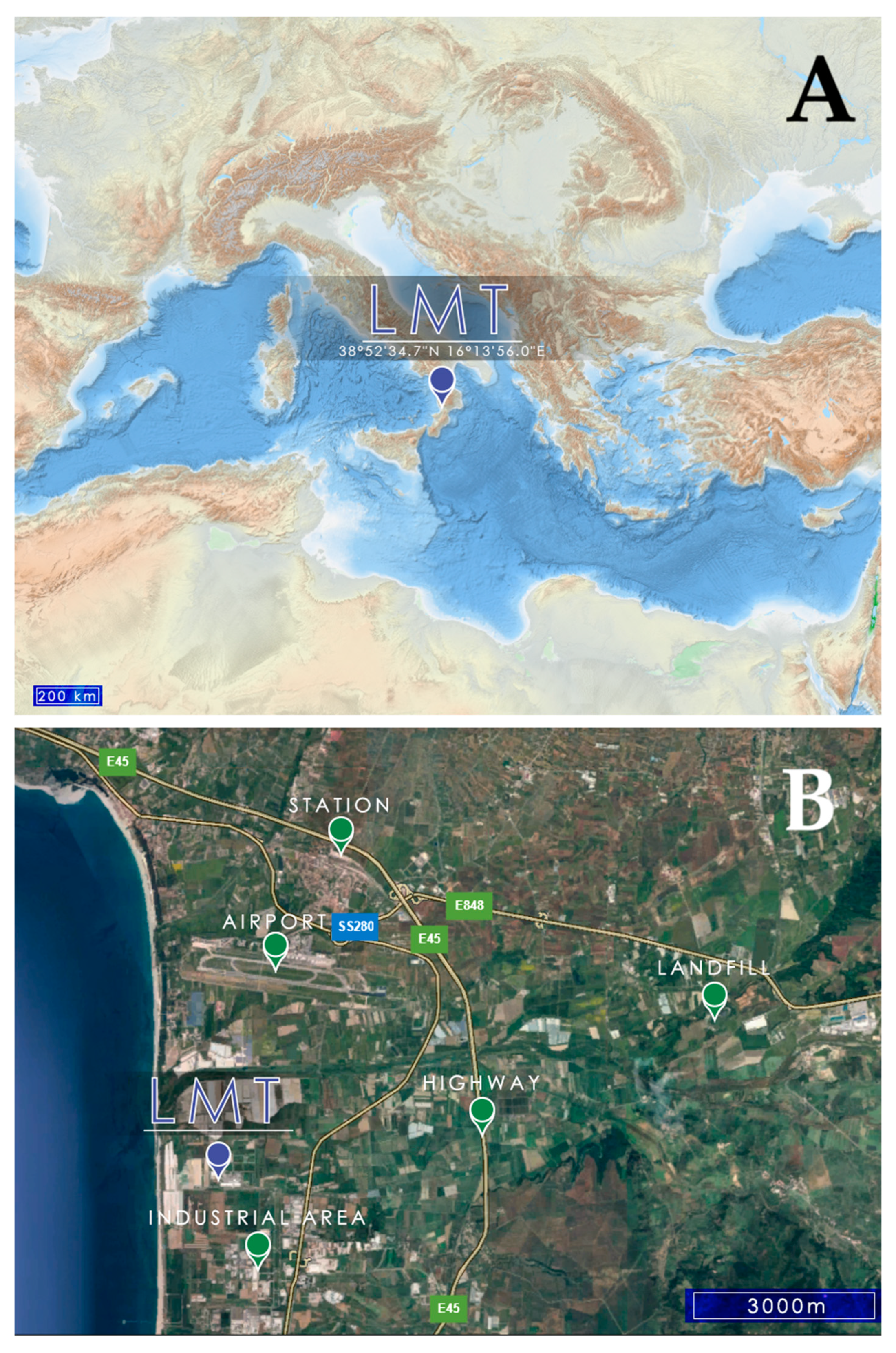
Figure 2.
Wind rose correlating the main proximity categories LOC, N–SRC, R–SRC, BKG, R–SRCcor, and BKGcor with directions and speeds observed at the LMT site. The two “cor” categories are shown as triangles. This evaluation is based on the “Proximity Meteo” dataset (Table 1) which combines the measurements of Vaisala WXT520, Thermo 42i, Thermo 49, and Picarro G2401 instruments.
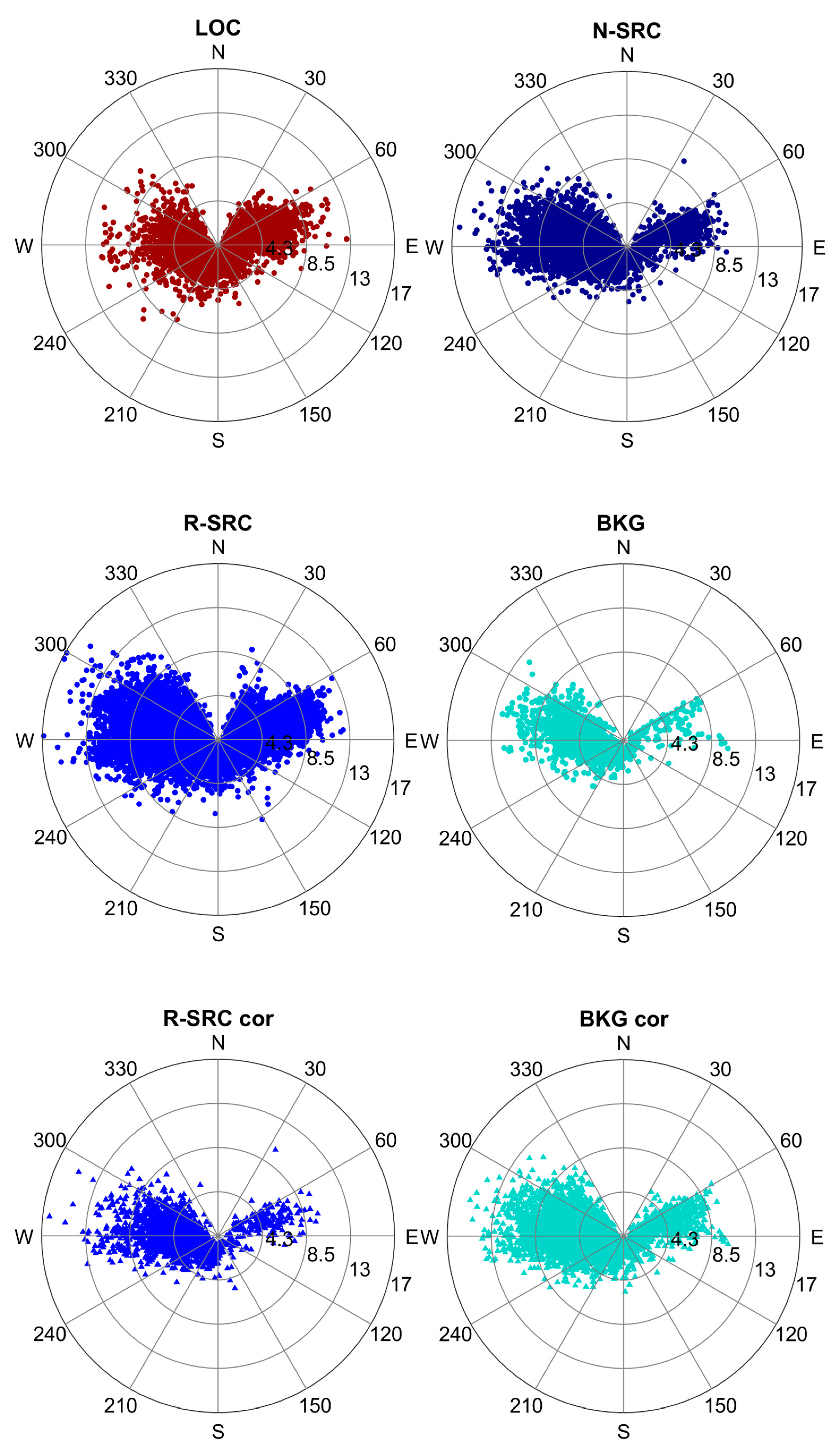
Figure 3.
Daily cycle of carbon monoxide (CO, ppb) under different proximity categories and seasons (Winter = black; Spring = green; Summer = red; Fall = yellow). A: LOC; B: N–SRC; C: R–SRC; D: BKG; E: corrected R–SRC; F: corrected BKG. Enhanced corrections (ecor) for Spring and Summer are shown as dashed lines in E and F.
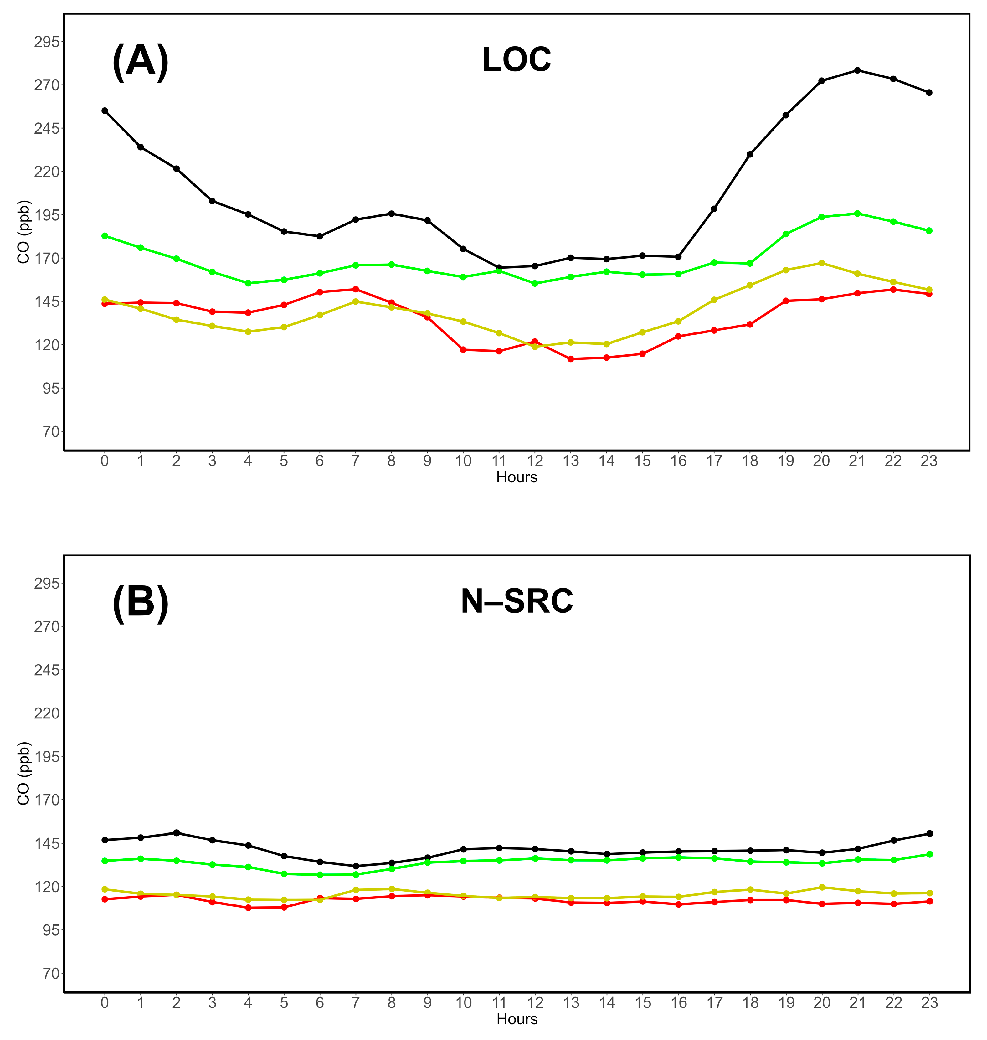
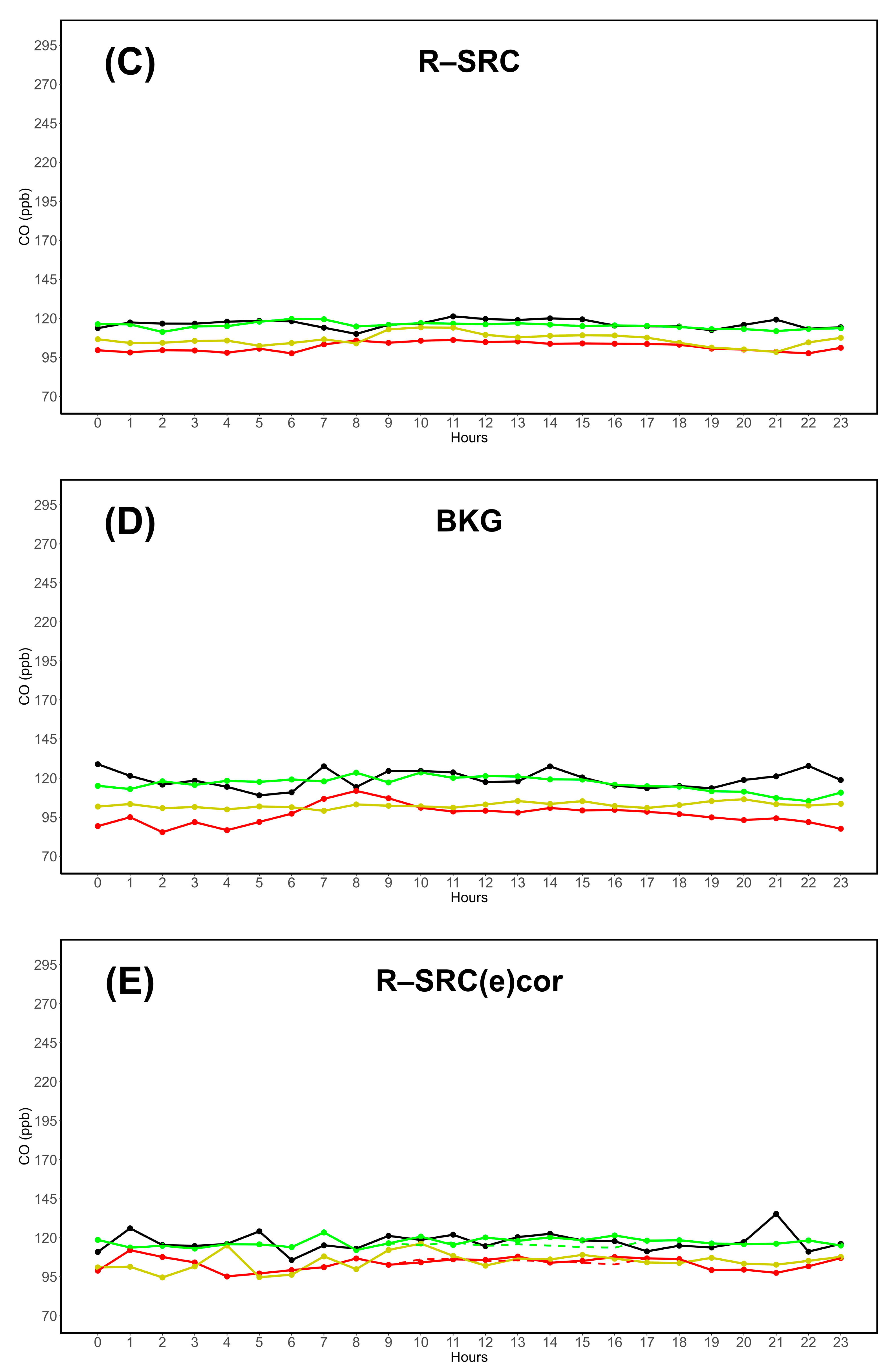
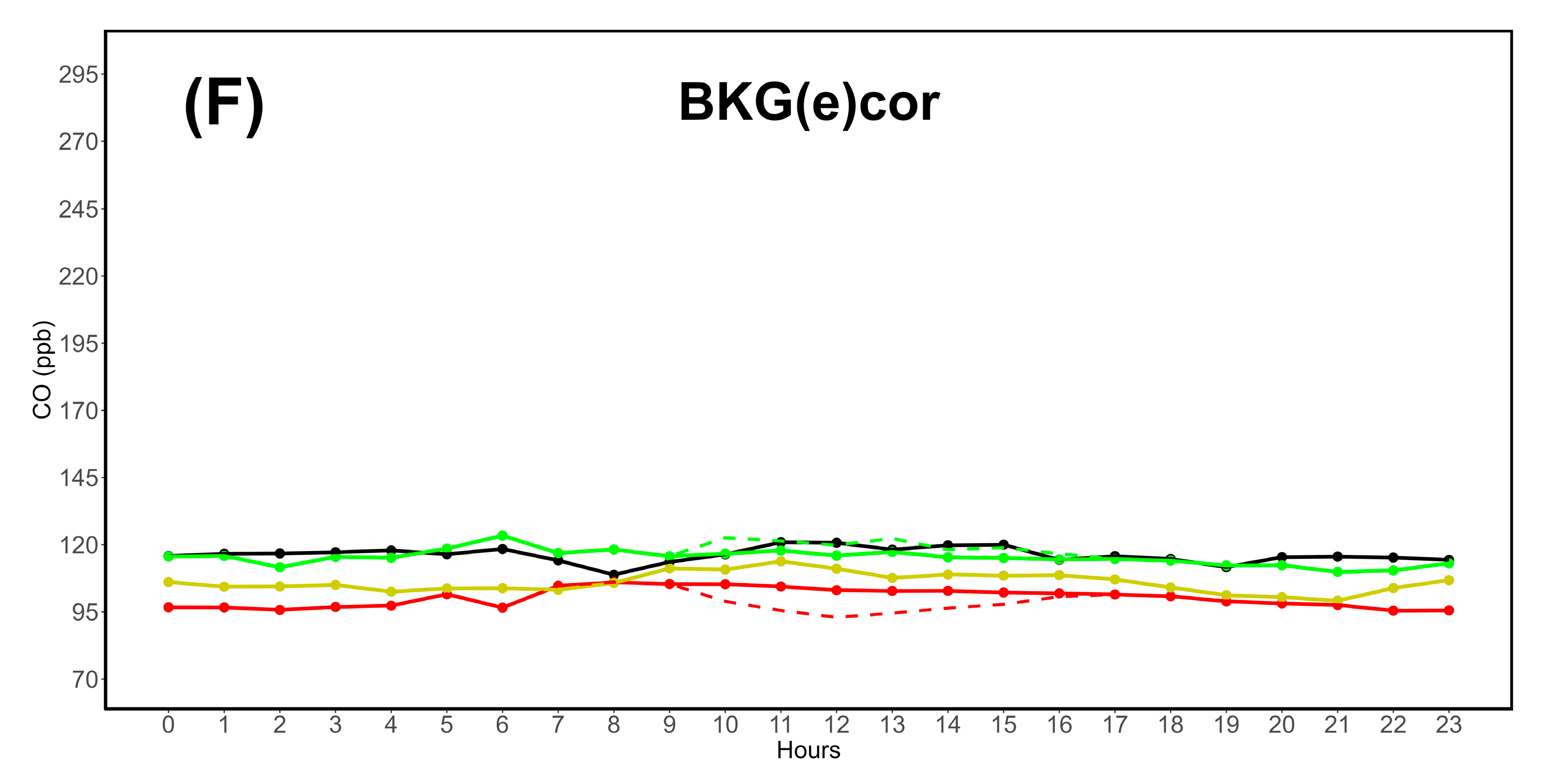
Figure 4.
Daily cycle of carbon dioxide (CO2, ppm) under different proximity categories and seasons (Winter = black; Spring = green; Summer = red; Fall = yellow). A: LOC; B: N–SRC; C: R–SRC; D: BKG; E: corrected R–SRC; F: corrected BKG. Enhanced corrections (ecor) for Spring and Summer are shown as dashed lines in E and F.
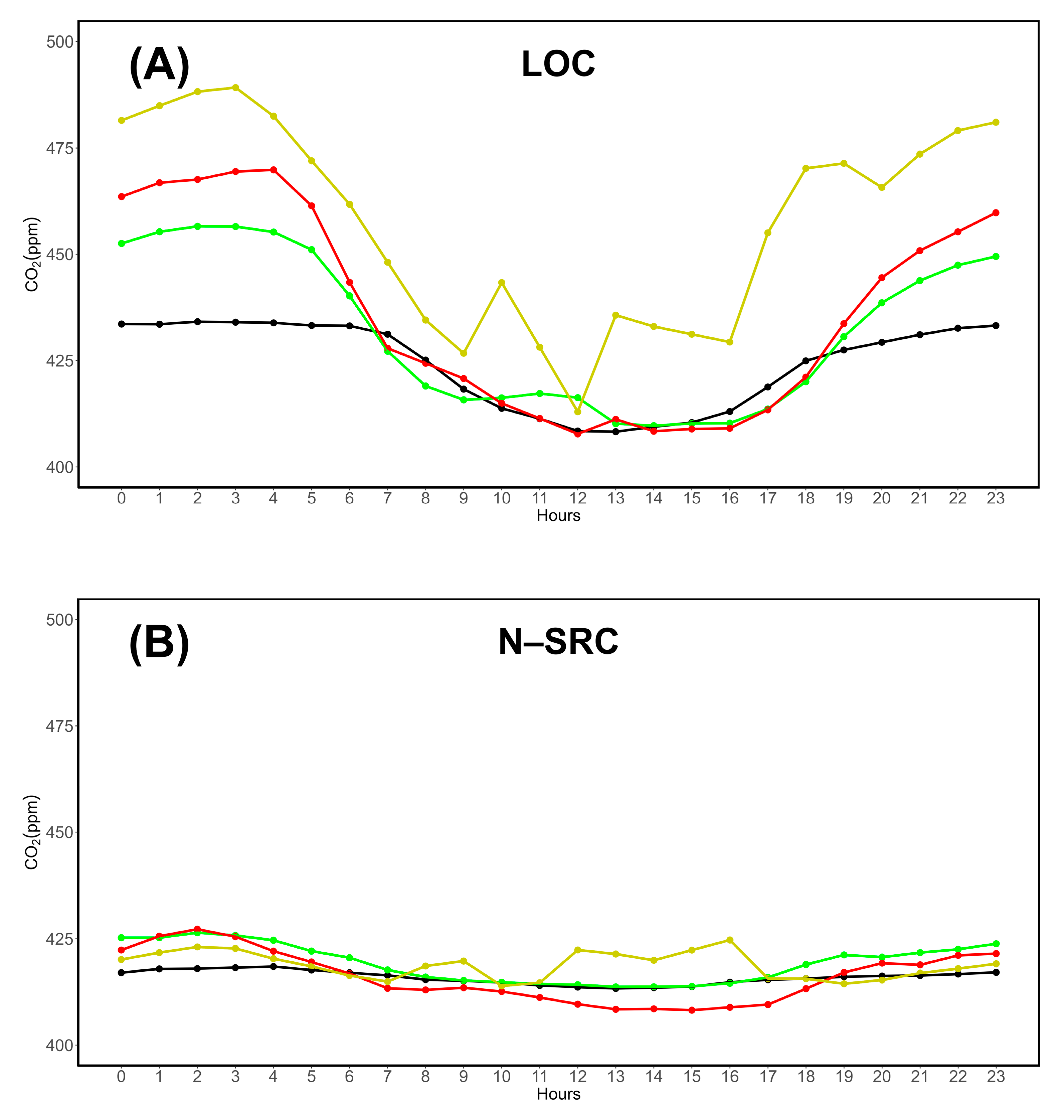
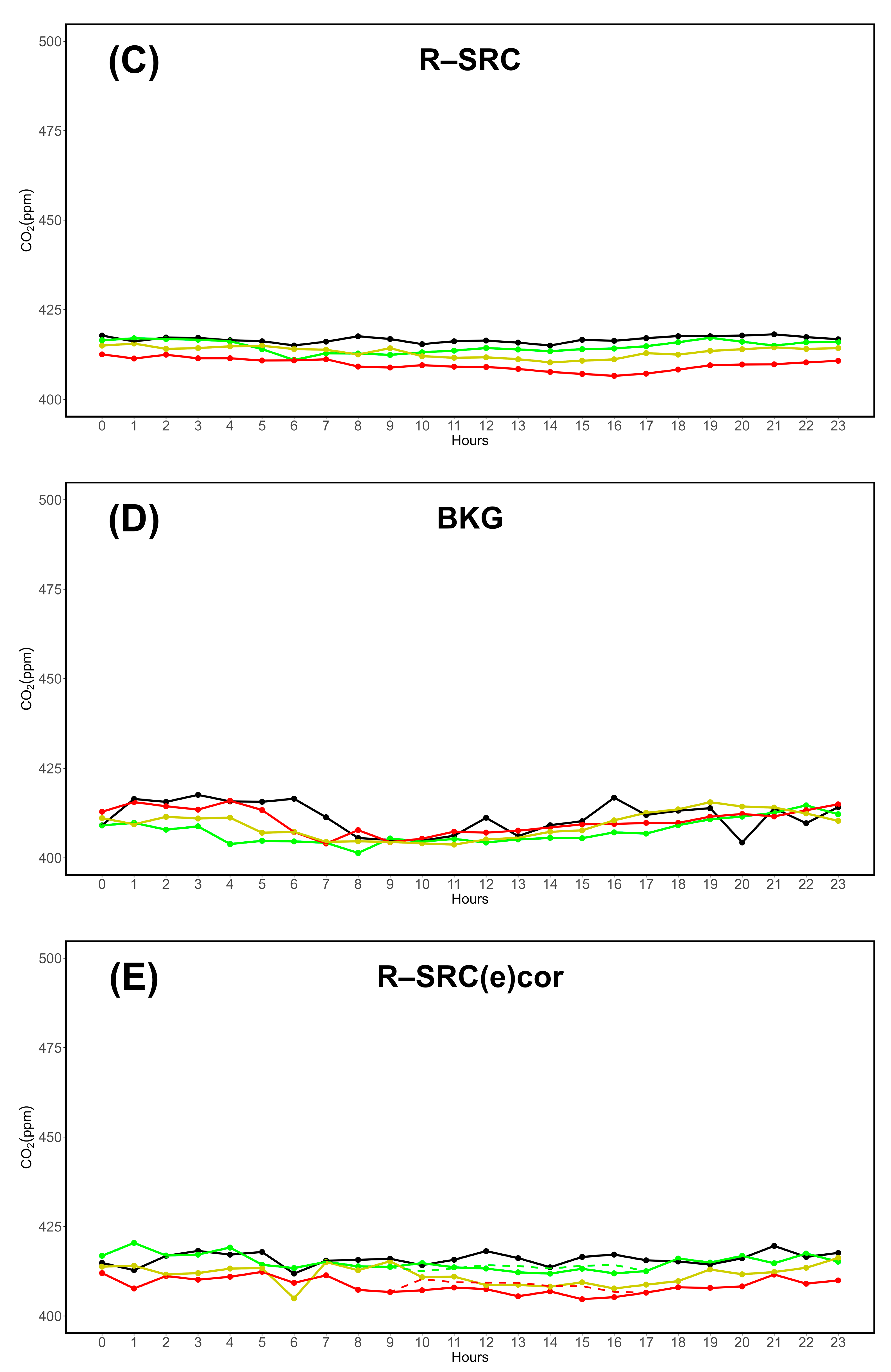
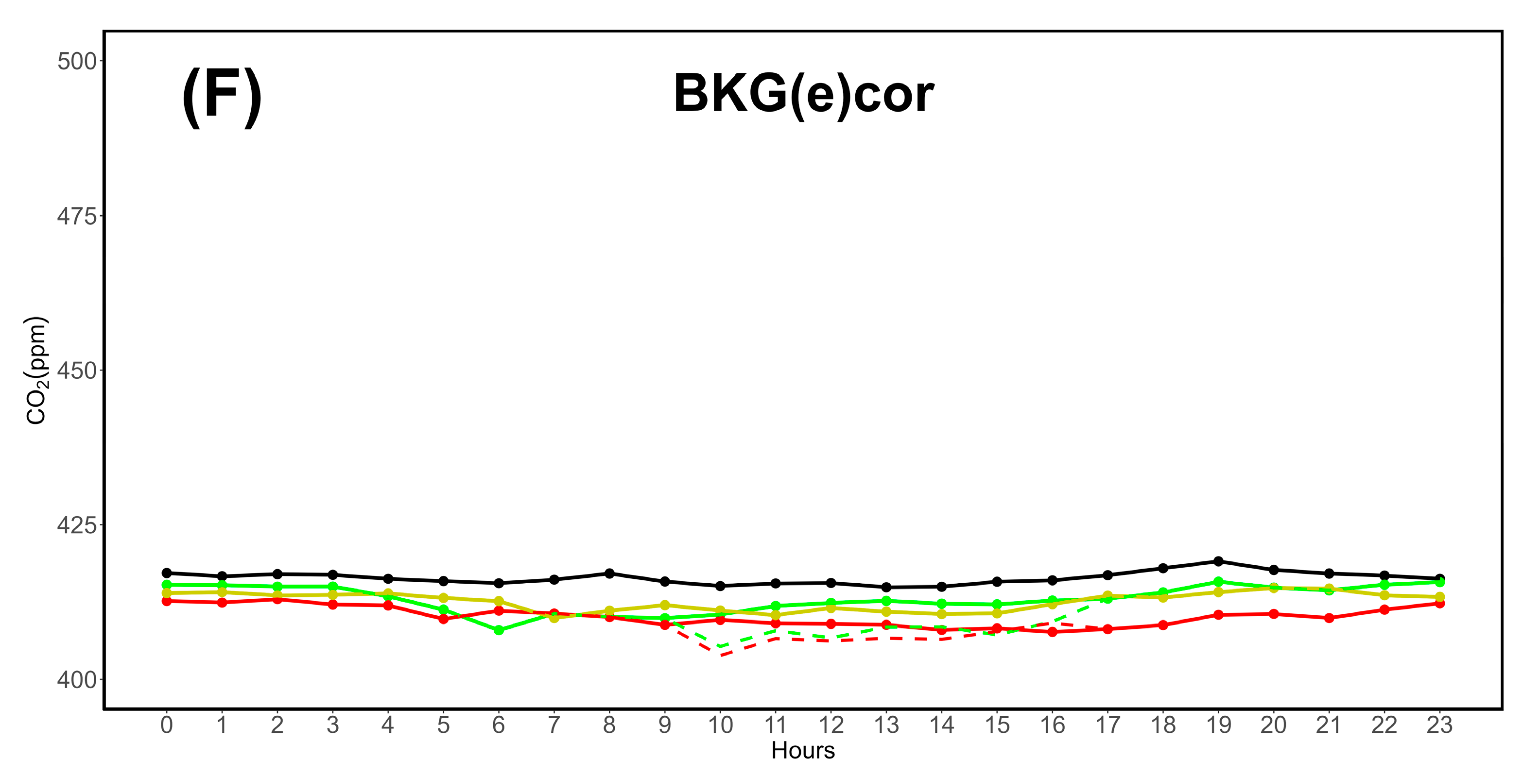
Figure 5.
Daily cycle of methane (CH4, ppb) under different proximity categories and seasons (Winter = black; Spring = green; Summer = red; Fall = yellow). A: LOC; B: N–SRC; C: R–SRC; D: BKG; E: corrected R–SRC; F: corrected BKG. Enhanced corrections (ecor) for Spring and Summer are shown as dashed lines in E and F.
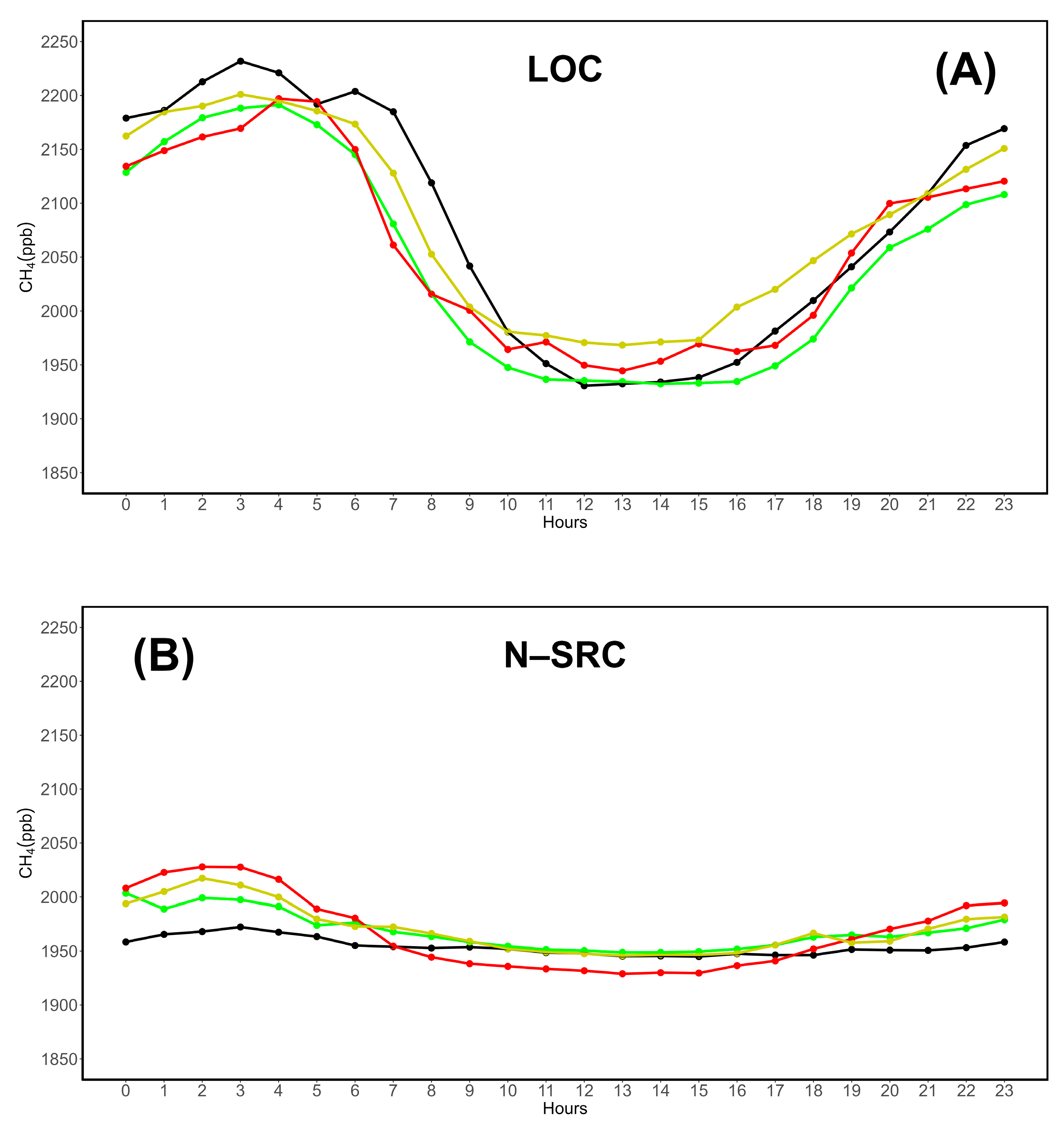
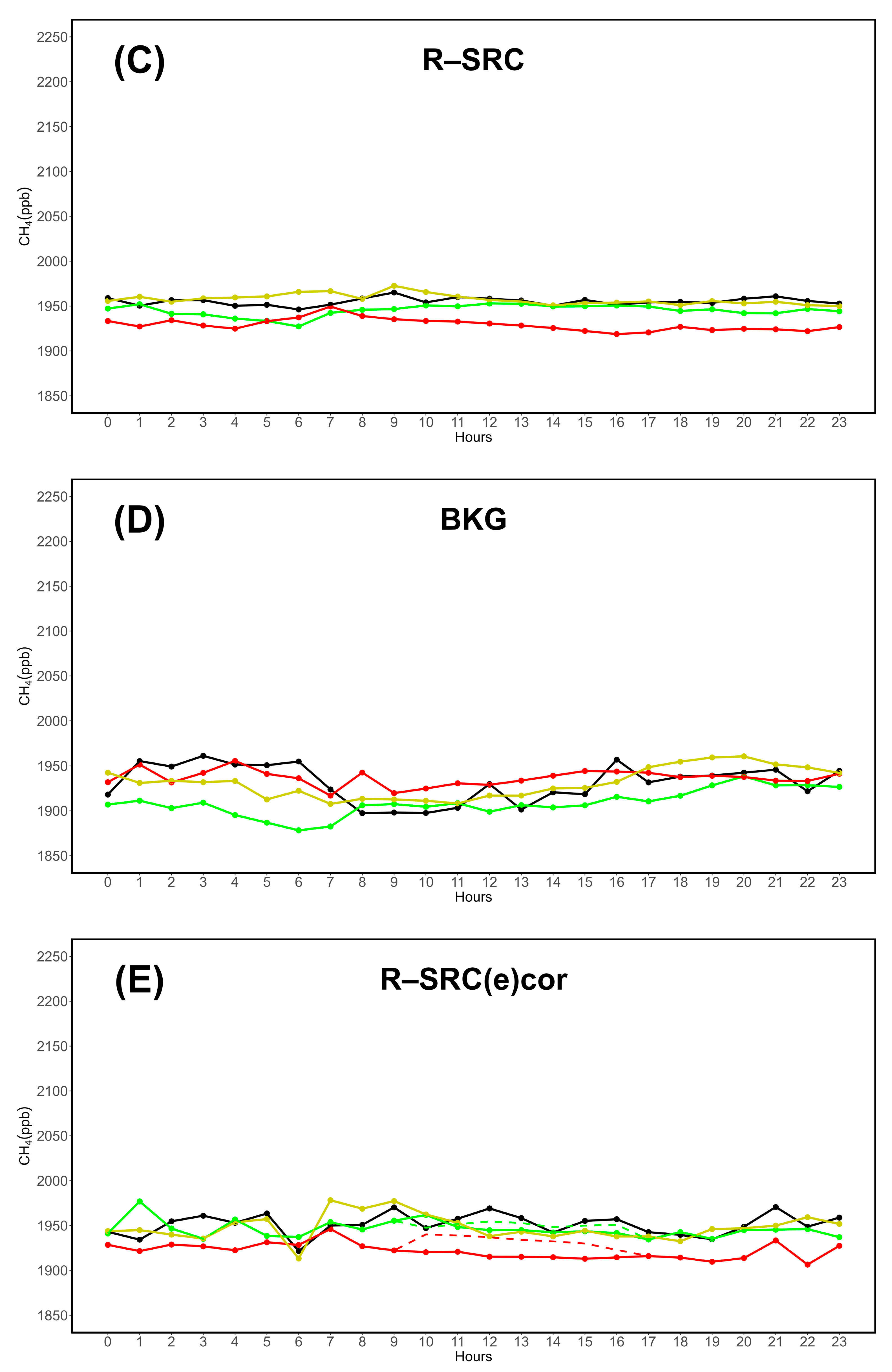

Figure 12.
Evaluation of CO concentrations in ppb under different wind corridors at the LMT site. A: northeast or “continental” sector, defined in the 0-90 °N range; B: western or “seaside” corridor, in the 240-300 °N range; C: all data, featuring the two above-mentioned corridors as well as the measurements falling outside the two ranges.
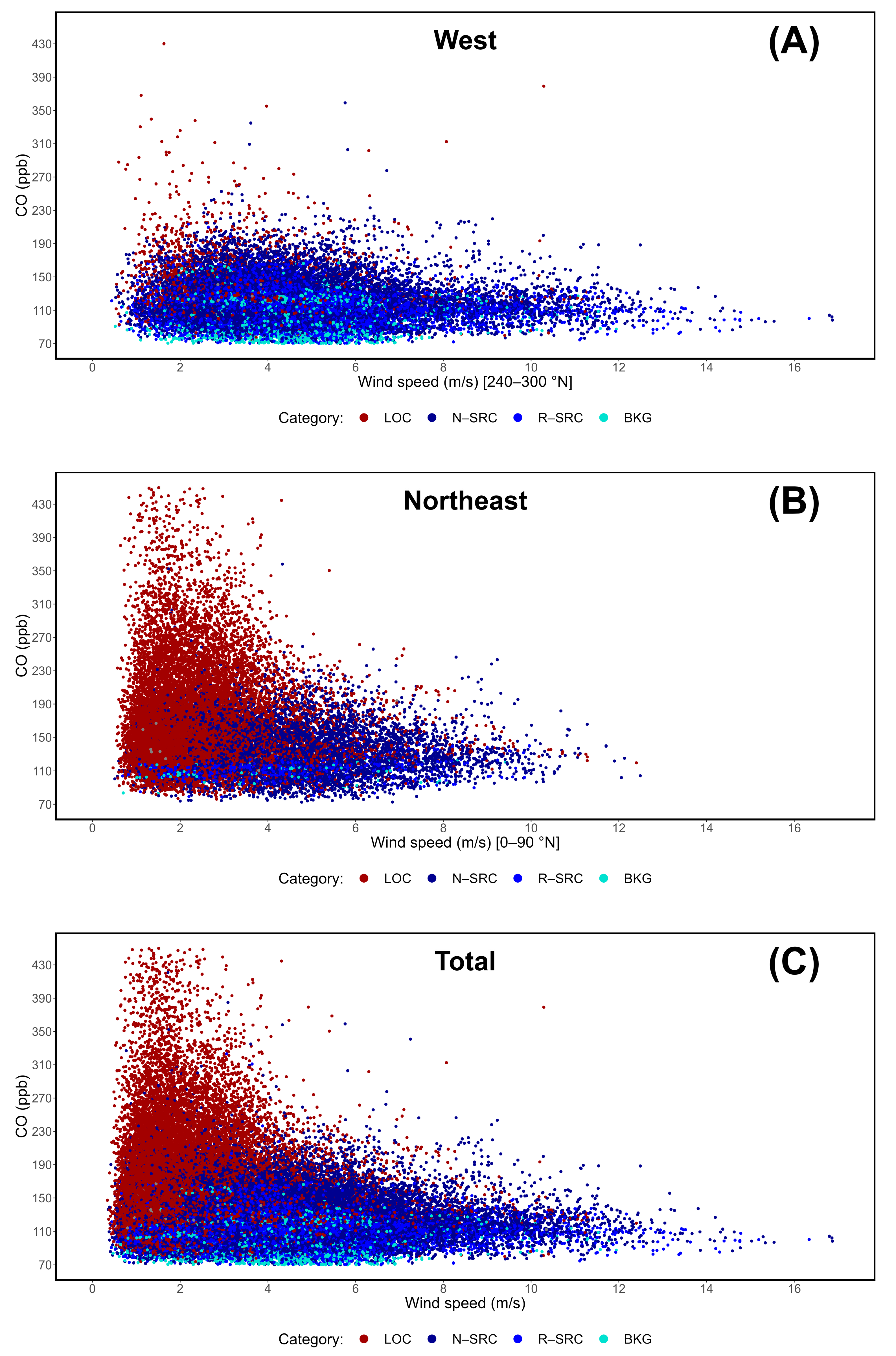
Figure 13.
Evaluation of CO2 concentrations in ppm under different wind corridors at the LMT site. A: northeast or “continental” sector, defined in the 0-90 °N range; B: western or “seaside” corridor, in the 240-300 °N range; C: all data, featuring the two above-mentioned corridors as well as the measurements falling outside the two ranges.
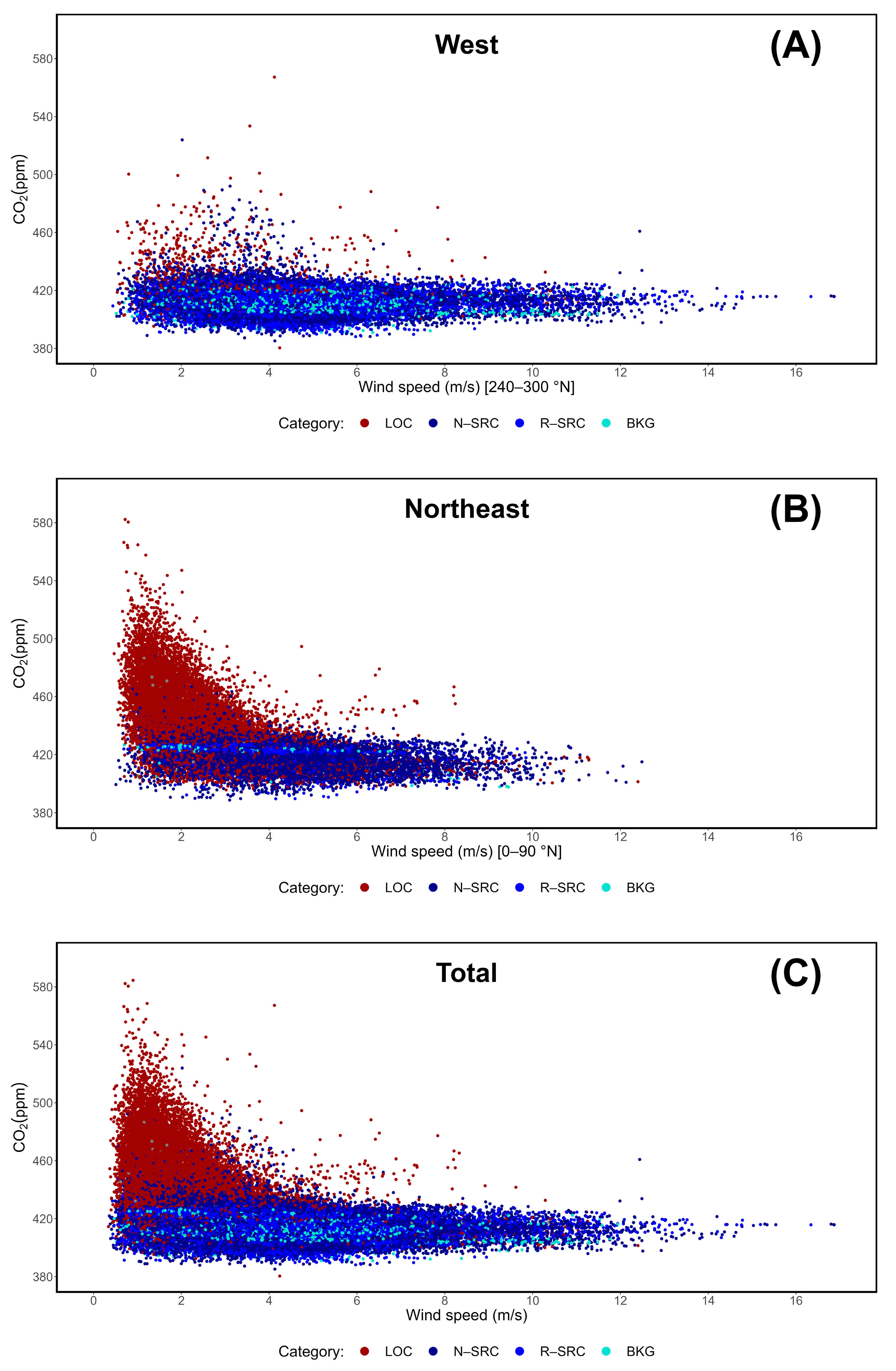
Figure 14.
Evaluation of CH4 concentrations in ppb under different wind corridors at the LMT site. A: northeast or “continental” sector, defined in the 0-90 °N range; B: western or “seaside” corridor, in the 240-300 °N range; C: all data, featuring the two above-mentioned corridors as well as the measurements falling outside the two ranges.

Figure 15.
Infra-annual cycles of CO (A), CO2 (B), and CH4 (C) based on averaged monthly concentrations, differentiated by proximity category. Dotted blue and turquoise lines show the variability in R–SRCcor and BKGcor, respectively. Dashed lines of the same colors show “ecor” values between March and August.
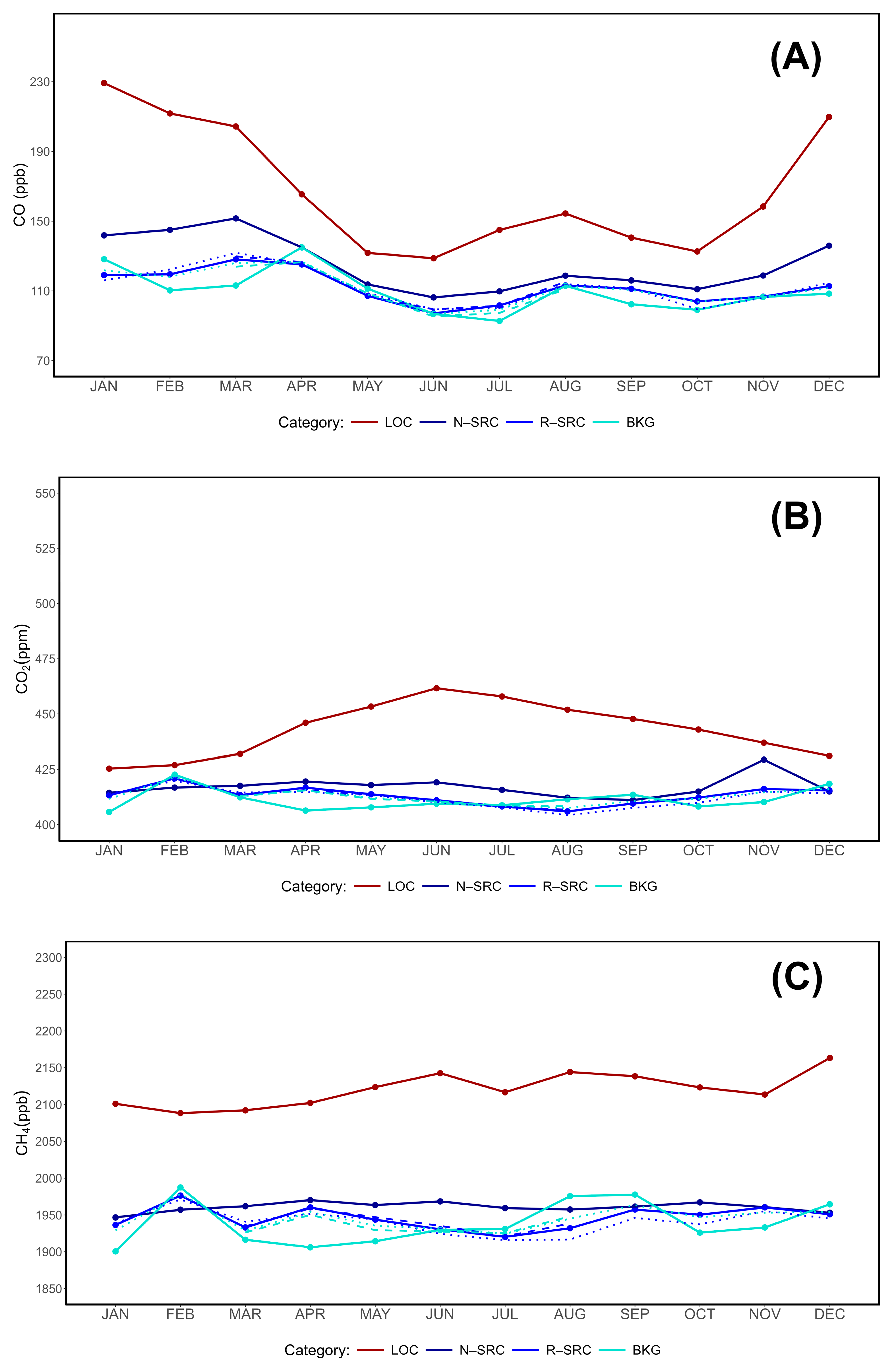
Figure 16.
Multi-year variability (2015-2023) reported by monthly averages of CO (A), CO2 (B), and CH4 (C), differentiated by proximity category. Dotted blue and turquoise lines show the variability in R–SRCcor and BKGcor, respectively. Dashed lines of the same colors show “ecor” values between March and August.
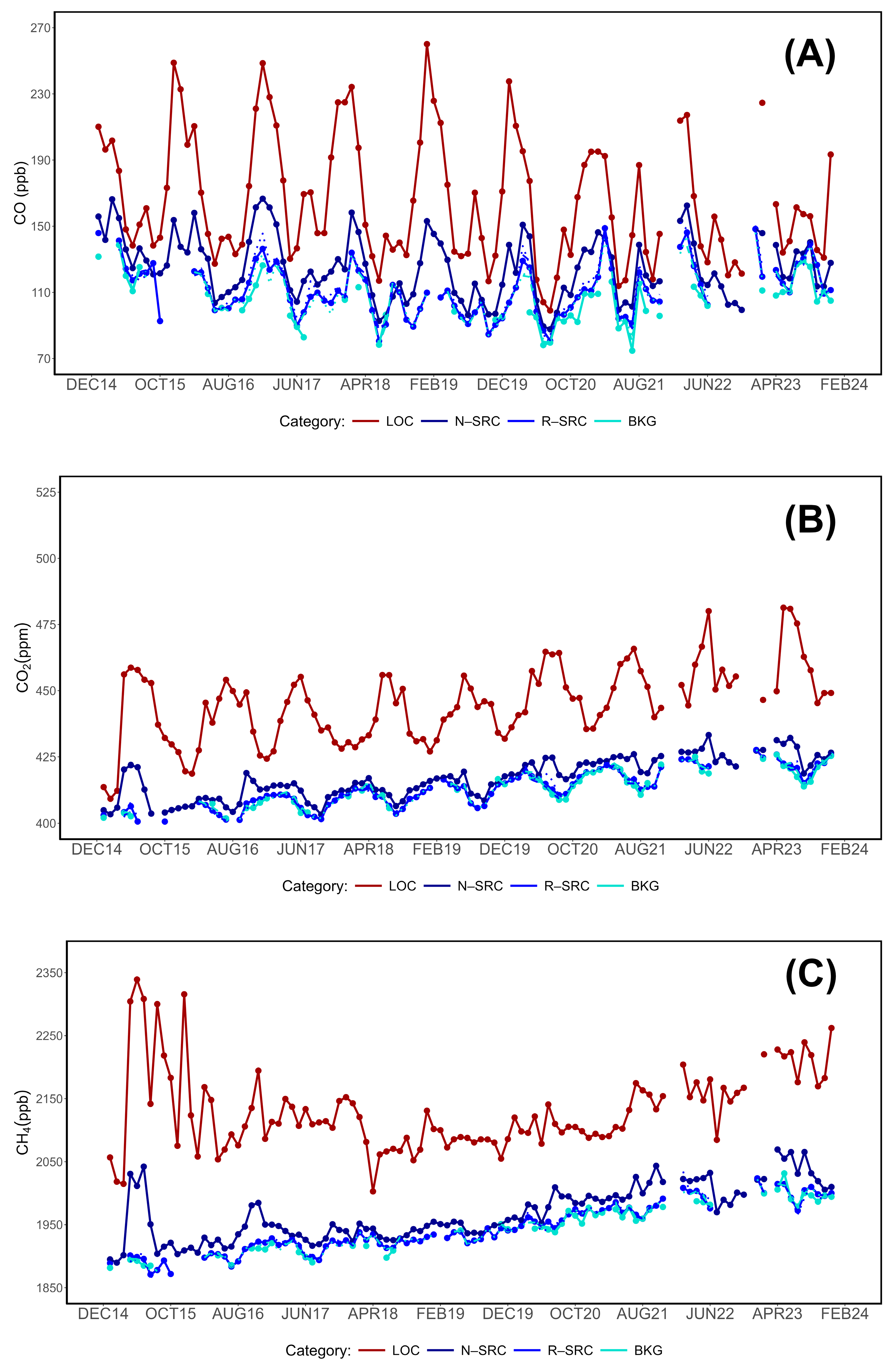

Table 1.
Yearly and total coverage rates of instruments and datasets, shown as percentages (%) compared to the actual number of hours elapsed between 2015 and 2023. Please note that both 2016 and 2020 were leap years, with an additional 24 hours. The “Preliminary” column refers to the combined Thermo 42i and 49i dataset with applicable O3/NOx ratios. “Proximity” refers to the subset of this set featuring valid Picarro G2401 data. “Proximity Meteo” also includes Vaisala WXT520 data.
| Year | Hours | G2401 | T42i | T49i | WXT520 | Prelim. | Proximity | Prox. Meteo |
|---|---|---|---|---|---|---|---|---|
| 2015 | 8760 | 94.73% | 92.73% | 92.14% | 95.9% | 92.12% | 87.87% | 86.99% |
| 2016 | 8784 | 94.95% | 95.91% | 96.17% | 96.34% | 94.17% | 89.9% | 88.22% |
| 2017 | 8760 | 99.57% | 96.39% | 95.93% | 93.8% | 95.65% | 95.27% | 90.67% |
| 2018 | 8760 | 94% | 98.11% | 98.13% | 77.05% | 97.95% | 92.32% | 73.34% |
| 2019 | 8760 | 97.6% | 96.78% | 94.21% | 98.59% | 94.18% | 93.28% | 93.26% |
| 2020 | 8784 | 93.8% | 94.23% | 98.52% | 99.98% | 94% | 89.13% | 89.12% |
| 2021 | 8760 | 97.78% | 87.14% | 91.65% | 99.74% | 78.91% | 77.84% | 77.83% |
| 2022 | 8760 | 83.89% | 69% | 85.22% | 90.11% | 68.97% | 59.15% | 58.04% |
| 2023 | 8760 | 66.76% | 81.86% | 82.12% | 96.3% | 81.82% | 58.61% | 57.35% |
| 788881 | 91.45%2 | 90.24%2 | 92.68%2 | 94.20%2 | 88.64%2 | 82.60%2 | 79.42%2 |
1 Sum. 2 Average value.
Table 2.
Percentage (%) of hours falling into the six proximity categories (including the two corrected remote source, R–SRC, and background, BKG, sets), calculated from the “Preliminary” dataset shown in Table 1. To ease visualization and comparisons between coverage rates observed throughout the years, the same “Preliminary” column from Table 1 has been added to this table.
| Year | Prelim. | Standard | Corrected | ||||||
|---|---|---|---|---|---|---|---|---|---|
| LOC | N–SRC | R–SRC | BKG | R–SRCcor | BKGcor | R–SRCecor | BKGecor | ||
| 2015 | 92.12% | 48.97% | 30.54% | 10.75% | 9.71% | 2.78% | 17.68% | 6.24% | 13.39% |
| 2016 | 94.17% | 30.75% | 46.78% | 19.1% | 3.32% | 5.06% | 17.38% | 6.66% | 13.75% |
| 2017 | 95.65% | 36.65% | 45.49% | 16.95% | 0.89% | 4.6% | 13.24% | 7.49% | 8.67% |
| 2018 | 97.95% | 42.82% | 47.72% | 9.17% | 0.26% | 3.36% | 6.07% | 3.5% | 5.62% |
| 2019 | 94.18% | 42% | 45.99% | 11.92% | 0.07% | 3.84% | 8.15% | 5% | 5.46% |
| 2020 | 94% | 37.48% | 39.28% | 15.74% | 7.48% | 2.51% | 20.7% | 6.12% | 16.6% |
| 2021 | 78.91% | 34.7% | 40.72% | 19.39% | 4.55% | 4.09% | 19.86% | 9.18% | 13.61% |
| 2022 | 68.97% | 44.75% | 42.75% | 11.51% | 0.95% | 2.33% | 10.14% | 6.27% | 5.16% |
| 2023 | 81.82% | 33.31% | 34.96% | 26.15% | 5.35% | 4.43% | 27.07% | 10.86% | 19.51% |
| 88.64%1 | 39.05%1 | 41.58%1 | 15.63%1 | 3.62%1 | 3.67%1 | 15.59%1 | 6.81%1 | 11.31%1 | |
1 Average.
Table 3.
Comparison between R–SRC/BKG data and their corrected values based on the standard NO2/2 correction seen in Cristofanelli et al. (2017) [60] and the select O3/2 correction applied in this study, based on the findings of D’Amico et al. (2024d) [61]. Hereby reported are the differences between the standard values seen in Table 2 and the corrected values from the same table, as well as the differences between the two correction types.
| Year | Standard – cor | Standard – ecor | cor - ecor | |||
|---|---|---|---|---|---|---|
| R–SRC | BKG | R–SRC | BKG | R–SRC | BKG | |
| 2015 | -7.97% | +7.97% | -4.51% | +3.68% | +3.46% | -4.29% |
| 2016 | -14.04% | +14.06% | -12.44% | +10.43% | +1.6% | -3.63% |
| 2017 | -12.35% | +12.35% | -9.46% | +7.78% | +2.89% | -4.57% |
| 2018 | -5.81% | +5.81% | -5.67% | +5.36% | +0.14% | -0.45% |
| 2019 | -8.08% | +8.08% | -6.92% | +5.39% | +1.16% | -2.69% |
| 2020 | -13.23% | +13.22% | -9.62% | +9.12% | +3.61% | -4.1% |
| 2021 | -15.3% | +15.31% | -10.21% | +9.06% | +5.09% | -6.25% |
| 2022 | -9.18% | +9.19% | -5.24% | +4.21% | +3.94% | -4.98% |
| 2023 | -21.72% | +21.72% | -15.29% | +14.16% | +6.43% | -7.56% |
| -11,96%1 | +11,97%1 | -8,82%1 | +7,69%1 | +3.15%1 | -4.28%1 | |
1 Average.
Table 4.
Average concentrations (± 1σ) of CO (ppb), CO2 (ppm), and CH4 (ppb), per category.
| Type | Category | CO (ppb) | CO2 (ppm) | CH4 (ppb) |
|---|---|---|---|---|
|
Standard |
LOC | 170.360 ± 68.34 | 449.053 ± 217.56 | 2120.146 ± 187.49 |
| N–SRC | 126.492 ± 29.35 | 416.995 ± 53.22 | 1960.652 ± 67.33 | |
| R–SRC | 108.729 ± 19.29 | 411.788 ± 8.54 | 1940.776 ± 43.06 | |
| BKG | 103.882 ± 21.01 | 409.174 ± 7.85 | 1930.955 ± 42.39 | |
|
Corrected |
R–SRCcor | 110.217 ± 18.67 | 410.817 ± 8.38 | 1935.428 ± 41.15 |
| BKGcor | 107.194 ± 19.94 | 411.395 ± 8.49 | 1939.720 ± 43.53 | |
| R–SRCecor | 108.681 ± 19.57 | 410.874 ± 8.91 | 1939.121 ± 42.55 | |
| BKGecor | 106.957 ± 19.84 | 411.757 ± 8.12 | 1939.934 ± 43.51 |
Table 5.
Average concentrations (± 1σ) of CO (ppb), CO2 (ppm), and CH4 (ppb), divided by category and season. Fall and Winter concentrations of “ecor” categories are omitted as they are identical to their “cor” counterparts.
Table 5.
Average concentrations (± 1σ) of CO (ppb), CO2 (ppm), and CH4 (ppb), divided by category and season. Fall and Winter concentrations of “ecor” categories are omitted as they are identical to their “cor” counterparts.
| Category | Season | CO (ppb) | CO2 (ppm) | CH4 (ppb) |
|---|---|---|---|---|
|
LOC |
Fall | 143.803 ± 48.42 | 468.575 ± 395.02 | 2125.003 ± 165.83 |
| Spring | 172.361 ± 54.17 | 442.211 ± 25.07 | 2103.867 ± 182.11 | |
| Summer | 144.902 ± 50.36 | 456.226 ± 26.16 | 2135.630 ± 176.26 | |
| Winter | 217.324 ± 82.18 | 427.627 ± 15.99 | 2115.857 ± 218.65 | |
|
N–SRC |
Fall | 115.183 ± 23.05 | 418.406 ± 104.13 | 1963.134 ± 65.08 |
| Spring | 134.058 ± 25.49 | 418.273 ± 9.64 | 1964.990 ± 66.35 | |
| Summer | 112.362 ± 25.35 | 415.267 ± 13.34 | 1961.091 ± 89.99 | |
| Winter | 141.453 ± 32.36 | 415.512 ± 6.99 | 1952.578 ± 42.87 | |
|
R–SRC |
Fall | 107.461 ± 17.21 | 412.358 ± 7.03 | 1955.852 ± 36.57 |
| Spring | 115.245 ± 16.47 | 414.629 ± 7.44 | 1947.553 ± 41.44 | |
| Summer | 103.248 ± 20.49 | 408.617 ± 8.99 | 1927.197 ± 44.45 | |
| Winter | 116.777 ± 15.99 | 416.625 ± 6.14 | 1954.998 ± 33.49 | |
|
BKG |
Fall | 102.842 ± 10.85 | 409.531 ± 6.78 | 1932.981 ± 35.15 |
| Spring | 116.123 ± 16.96 | 407.519 ± 8.08 | 1912.625 ± 44.08 | |
| Summer | 97.822 ± 22.30 | 409.510 ± 7.78 | 1937.851 ± 40.86 | |
| Winter | 118.304 ± 12.96 | 412.611 ± 9.06 | 1935.331 ± 45.84 | |
|
R–SRCcor |
Fall | 106.273 ± 16.24 | 410.081 ± 7.14 | 1945.307 ± 36.28 |
| Spring | 117.803 ± 16.14 | 414.033 ± 7.71 | 1945.937 ± 42.82 | |
| Summer | 104.525 ± 19.25 | 407.336 ± 8.43 | 1918.533 ± 38.25 | |
| Winter | 117.730 ± 17.04 | 415.991 ± 5.64 | 1951.843 ± 33.81 | |
|
BKGcor |
Fall | 106.782 ± 16.43 | 412.381 ± 6.96 | 1953.807 ± 37.42 |
| Spring | 114.771 ± 16.62 | 413.182 ± 8.11 | 1940.098 ± 44.24 | |
| Summer | 101.455 ± 21.37 | 409.133 ± 8.76 | 1931.988 ± 44.60 | |
| Winter | 116.630 ± 15.31 | 416.383 ± 6.81 | 1953.831 ± 35.54 | |
|
R–SRCecor |
Fall | - | - | - |
| Spring | 115.289 ± 16.81 | 414.143 ± 7.49 | 1949.402 ± 42.19 | |
| Summer | 104.523 ± 20.48 | 408.654 ± 9.46 | 1930.893 ± 43.18 | |
| Winter | - | - | - | |
|
BKGecor |
Fall | - | - | - |
| Spring | 114.889 ± 16.27 | 412.867 ± 8.43 | 1934.997 ± 45.01 | |
| Summer | 99.403 ± 21.52 | 409.309 ± 8.07 | 1930.839 ± 44.99 | |
| Winter | - | - | - |
Disclaimer/Publisher’s Note: The statements, opinions and data contained in all publications are solely those of the individual author(s) and contributor(s) and not of MDPI and/or the editor(s). MDPI and/or the editor(s) disclaim responsibility for any injury to people or property resulting from any ideas, methods, instructions or products referred to in the content. |
© 2025 by the authors. Licensee MDPI, Basel, Switzerland. This article is an open access article distributed under the terms and conditions of the Creative Commons Attribution (CC BY) license (http://creativecommons.org/licenses/by/4.0/).
Copyright: This open access article is published under a Creative Commons CC BY 4.0 license, which permit the free download, distribution, and reuse, provided that the author and preprint are cited in any reuse.


