
Submitted:
29 April 2025
Posted:
30 April 2025
You are already at the latest version
Abstract
The photochemical production of tropospheric ozone (O3) is very closely linked to seasonal cycles and peaks in solar radiation occurring during warm seasons. In the Mediterranean Basin, which is a hotspot for climate and air mass transport mechanisms, boreal warm seasons cause a notable increase in tropospheric O3, which unlike stratospheric O3, is not beneficial for the environment. At the Lamezia Terme (code: LMT) World Meteorological Organization – Global Atmosphere Watch (WMO/GAW) station located in Calabria, Southern Italy, peaks of stratospheric O3 were observed during boreal summer and spring seasons, and consequently linked to specific wind patterns compatible with increased photochemical activity in the Tyrrhenian Sea. The finding resulted in the introduction of a correction factor for O3 in the O3/NOx (ozone to nitrogen oxides) ratio methodology for the assessment of air mass aging. However, some of the mechanisms driving O3 patterns and their correlation with other parameters at the LMT site remain unknown. In this study, the behavior of O3 at the site is assessed with unprecedented detail by relying on nine years (2015-2023) of data and correlations with surface temperature and solar radiation. The evaluations demonstrate non negligible correlations between environmental factors such as temperature and solar radiation with O3 concentrations. The northeastern sector of LMT, partly neglected in previous works, has yielded higher statistical correlations than expected. A case study of very high O3 concentrations reported during the 2015 summer season is also reported by analyzing the tendencies observed during the period with additional methodologies and highlighting drivers of photochemical pollution on larger scales.
Keywords:
tropospheric ozone
; photochemical production
; Mediterranean Basin
; regional photochemical pollution
1. Introduction
Photochemical processes are a key driver in atmospheric chemistry [1], as well as in regular chemical dynamics [2]. Ozone (O3) is a reactive and oxidant gas, heavily influenced by photochemistry, discovered by Christian Friedrich Schönbein in the nineteenth century [3,4]. Following its discovery, O3 was proven to increase with altitude and show distinct behavior based on vertical gradients, thus leading to a well-defined differentiation between tropospheric O3 and stratospheric O3, with the latter being beneficial for the environment [5] as it reduces the impact of solar radiation on terrestrial ecosystems [6,7,8] while the former poses health issues to living organisms [9,10,11,12,13,14]. Stratospheric O3 depletion caused by anthropogenic emission has been the core issue of environmental policies for years, up until the implementation of adequate mitigation measures [15,16,17,18,19,20].
Tropospheric O3 has a concentration of a few dozen ppb (parts per billion), while stratospheric O3 peaks at 20-30 kilometers above ground level with concentrations of ≈10 ppm (parts per million) [21,22,23,24,25,26]. STT (Stratosphere-to-Troposphere Transport) events may lead to SI (Stratospheric Intrusion) phenomena, and therefore increase tropospheric O3 under specific conditions [27,28,29,30,31,32].
The photochemical production of O3 has been the subject of research for decades [33,34,35,36,37,38,39]. Significant correlations between O3 production and the presence of other compounds in the atmosphere, such as VOCs (Volatile Organic Compounds) have also been reported across the globe [40,41,42,43,44,45].
Among the drivers of O3 production in the atmosphere are photo oxidation mechanisms triggered by nitrogen oxides (NO + NO2 = NOx) and affecting the above mentioned VOCs; NMVOCs (Non Methane VOCs) and NOx may be the result of natural activities and anthropogenic emissions, however it is worth mentioning that the mechanisms leading to O3 production may vary in nature [46,47] due to chemical reactions – specifically, titration - resulting in NO2 increases from NO [48,49]. Two of the main carbon compounds present in the atmosphere, CO (carbon monoxide) and CH4 (methane), are also connected to tropospheric O3 production [50]. Intense solar radiation, which in the context of the Mediterranean Basin are primarily linked with boreal summer seasons, are known to intensify O3 production [46]; specifically, several works have highlighted the exposure of southern European regions to these processes, thus sparking notable interest on the topic of regional photochemical pollution in the Mediterranean [51,52,53,54,55,56,57,58,59,60].
Increases in tropospheric O3 concentrations may be the result of the interplay of local-to-remote mechanisms, as air mass transport and photochemistry can result in tropospheric O3 increases far from the initial emission sources of O3 precursors; these effects have been observed over notable distances, crossing entire oceans [61], but are most notably reported on a continental scale [53,54,59,60,62,63]. The effects may be amplified in regions such as the Mediterranean, which is a known hotspot for climate, air quality, and air mass transport processes [64,65,66,67,68]. The Mediterranean is also known to be sensitive to various stresses, such as air pollution and water shortage [69,70]. The area is also characterized by differences between its eastern and western sectors affecting air circulation patterns [71,72].
These heterogeneities also result in peculiar sources of NOx and VOC emissions that drive O3 production and its consequent chemical reactions in the atmosphere [73,74,75,76] as well as the transport of air masses enriched in O3 [53,54,62,77]. Overall, the combination of the above-mentioned factors have allowed the Mediterranean Basin to be defined as a major hotspot for the study and evaluation of tropospheric O3, especially considering the reported differences in O3 variability between the eastern and western sectors of the basin itself [51,54,56,59,60,78,79,80,81,82,83,84,85,86,87,88,89,90,91,92,93,94].
In addition to the studies aimed at O3 patterns and variability over wide areas in the Mediterranean Basin, research has also focused specifically on the Italian peninsula [95,96,97]. At the World Meteorological Organization – Global Atmosphere Watch (WMO/GAW) observation site of Lamezia Terme (code: LMT) in southern region of Calabria, previous research has evidenced peaks in O3 concentrations attributable to enhanced photochemical activity [98]. The peaks have been considered in consequent research based on the ratio of O3 to NOx (nitrogen oxides) as a proximity and air mass aging indicator, by halving the reported concentration of O3 under specific conditions in order to compensate for photochemical production peaks [99]. This factor supplemented another correction meant to compensate for possible NO2 overestimation caused by the presence of heated molybdenum converters in NOx analyzers [100]. At LMT, the O3/NOx ratio has allowed to determine, with unprecedented accuracy, the balance of local, intermediate, and remote contributions to local measurements [98,100]. However, the mechanisms driving O3 increases are yet to be fully characterized at the site, especially with respect to environmental factors such as ground temperature and solar radiation. A more detailed understanding of these mechanisms can therefore integrate present-day knowledge on O3 behavior in the central Mediterranean, and also contribute towards the enhancement of the O3/NOx methodology, which in turn is necessary to better evaluate medium-to-long tendencies and variabilities of CO2 (carbon dioxide), CO, CH4, and other atmospheric compounds linked to anthropogenic emissions [101].
2. The Lamezia Terme Station and Employed Methods
2.1. The LMT WMO/GAW Observation Site in Calabria, Southern Italy
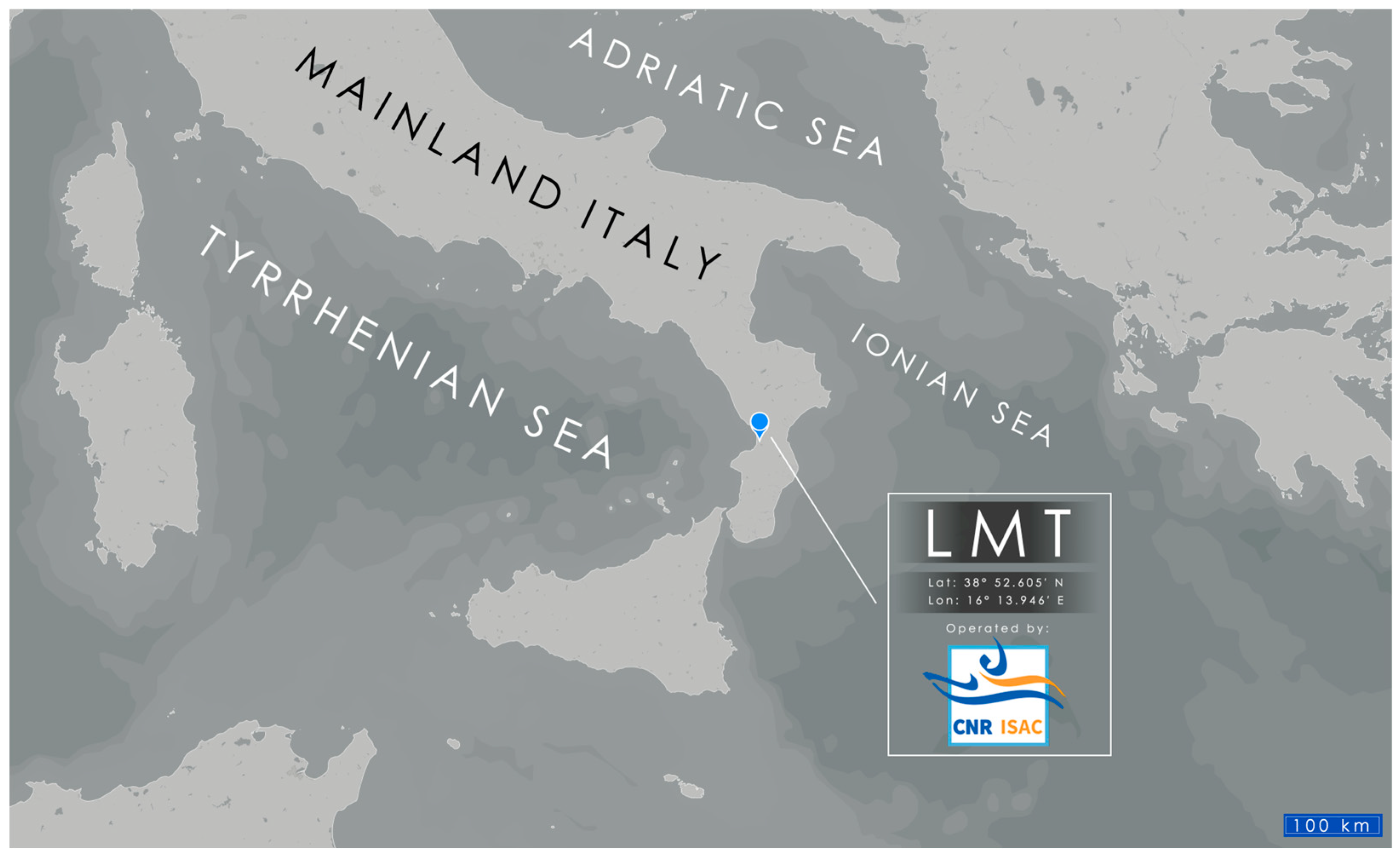
Located 600 meters from the Tyrrhenian coastline of Calabria (Italy), the Lamezia Terme (code: LMT; Lat: 8°52.605′ N; Lon: 16°13.946′ E; Elev: 6 meters AGL) observation site is part of the World Meteorological Organization – Global Atmosphere Watch (WMO/GAW) network and is fully operated by the National Research Council of Italy – Institute of Atmospheric Sciences and Climate (CNR-ISAC). The observation site is located in the industrial area of the Lamezia Terme municipality, within the province of Catanzaro. With a distance of ≈32 kilometers between the Tyrrhenian and Ionian coasts of the region, LMT is located in the westernmost sector of the narrowest point in the entire Italian peninsula, the Catanzaro isthmus. The isthmus effectively separates the Sant’Eufemia plain, where the observation is located, from southern (Serre Massif) and northern (Catena Costiera, Sila Massif) mountain ranges [102,103]. As a result of this peculiar geomorphological framework, near-surface winds are channeled through the isthmus [104], exploiting the depression caused by tectonics [105,106,107,108,109,110,111]. In the early Quaternary period, the isthmus accommodated a tidal strait directly connecting the two seas, as evidenced by local outcrops showing structures linked to 3D and 2D dunes [112,113,114].
The Calabrian Arc uplift triggered marine regression and transgression cycles [115,116,117,118,119,120,121] which combined with sea level variations induced by alternating interglacial and glacial periods [122,123,124], thus leading to the present-day configuration.
Figure 1.
Location of the LMT observation site in southern Italy, shown on a EUMETSAT [125] map.
Figure 1.
Location of the LMT observation site in southern Italy, shown on a EUMETSAT [125] map.
The unique geomorphological and orographic framework of the Catanzaro isthmus compared to the rest of the Italian peninsula allows near-surface wind circulation to be well oriented on a preferential W/NE axis as observed by the LMT observatory itself. Wind patterns are influenced by seasonal variability, breeze regimes, and eastern/western synoptic conditions, and have also showed vertical gradients reflecting large scale circulation in the area and local orography [126,127,128,129,130,131]. Breeze regimes were proven to be a key regulator of local climate and wind circulation, with seasonal variations being also reported; however, a primary W-WSW/NE-ENE axis dominates near-surface circulation, as a consequence of local orography; when considering the 850 hPa layer however, large scale flows in the area dominate with a preferred NW direction [126]. During most of the cold months, specifically between November and February, large scale forcing regulates diurnal wind circulation patterns; the March-October period is characterized by nighttime flows connected to nocturnal breeze regimes, and diurnal breezes resulting from both large scale and local flows [127].
LMT started data gathering operations in 2015. A preliminary study by Cristofanelli et al. (2017) provided the first data on O3 concentrations in the area, also accounting for the implementation of proximity categories based on the O3/NOx ratio [100]. This early work allowed to evaluate local sources of pollution, such as livestock farming in the Sant’Eufemia plain where LMT is located, as well as transportation contributions from the A2 highway and the Lamezia Terme International Airport (IATA: SUF; ICAO: LICA) located 2 km north of LMT. Consequently, an evaluation of several years of CH4 data (2016-2022) reported that northeastern-continental winds were enriched in anthropogenic outputs, while western-seaside winds generally yielded lower concentrations; higher concentrations were reported in winter, and lower concentrations during the summer [132].
The multi-year cyclic analysis of O3 (2015-2023) relied on a longer dataset to assess with greater detail O3 variability in the area, and demonstrated the presence of westerly peaks in concentrations linked to warm seasons, thus showing an opposite behavior compared to CH4 [98].
Due to its location in the central Mediterranean, LMT is subject to frequent dust episodes [133] and wildfire emissions [134], which peaked during the 2021 Mediterranean crisis due to large wildfires in the region of Calabria itself [135], as well as other locations in Italy and various countries overlooking the Mediterranean Basin [136]. Over the course of its operational history, the LMT station has been subject to comparative analyses aimed at multiple southern Italian atmospheric observatories, also accounting for aerosol optical properties and the influence of anthropic activities on measurements [137,138]. A study exploiting the strict restrictions applied by the Italian government during the first COVID-19 lockdown of 2020 [139,140] has allowed to pinpoint local emission sources with greater accuracy and validate previous hypotheses on said sources by evaluating circumstances of exceptionally low anthropogenic emissions [141].
2.2. Surface Measurements, Available Satellite Products, and Data Processing
At the LMT station, surface O3 mole fractions in ppb (parts per billion) have been measured by a Thermo Scientific 49i (Franklin, Massachusetts, USA), and instrument operating as a photometric analyzer [98]. The 49i model, operating with a precision of ±1 ppb O3 and a flow rate of 1-3 liters per minute (L/min), performs its measurements based on Beer-Lambert’s Law and, specifically, O3’s absorption of ultraviolet (UV) light at a wavelength of 254 nanometers (nm). Atmospheric O3 mole fractions are calculated from a comparison between the absorption occurring in a primary standard depleted in O3 by a scrubber, and the UV absorption at 254 nm in sampled air. The 49i instrument gathers ambient air and splits it in two distinct gas flows: the reference or standard gas used for the comparison passes through a pressure regulator, an O3 scrubber, and the standard solenoid valve; ambient air flows through the pressure regulator, the ozonator, and manifold to the sample solenoid valve. During measurements, the solenoid valves alternate the standard and ambient air streams between two cells, designated A and B, every 10 seconds. When one cell (for example, A) contains standard gas, the other (B) contains ambient air and vice versa. The 49i model measures UV light intensities in both cells; these measurements are interrupted for several seconds when the solenoid valves alternate between the two air flows. The interruption is necessary to ensure optimal flushing of both cells and prevent residual air from the previous flow to affect new measurements. The final output of ambient air O3 mole fractions is calculated, as per Beer Lambert’s Law, via the ratio of measured UV light intensities in ambient air and standard, O3 depleted, air. For the purpose of this research, hourly aggregates of O3 measurements in ppb have been used.
Surface measurements at the LMT site of downward solar radiation (W/m2) have been performed by a Kipp & Zonen CNR4 (Delft, Netherlands) radiometer. The instrument operates via two pyranometers and two pyrogeometers to measure downward (0.31–2.8 μm) and upward (4.5–42 μm) irradiance, respectively. As per the Baseline Surface Radiation Network (BSRN) standard, the uncertainty in these measurements is in the 1% range [142]. Previously gathered data at LMT has been studied for an early stage characterization of the site and a number of correlations with readily available products [143,144].
Key meteorological data on the surface have been gathered by a Vaisala WXT520 (Vantaa, Finland) weather station. Wind directions (WD, in degrees) and speeds (WS, in meters per second) are measured via ultrasounds transmitted, on a horizontal plane, between three transducers. Travel times of ultrasound pulses between transducers are altered by specific wind directions and speeds, which are measured by the instrument with a precision of ±3° and ±0.3 m/s, respectively. Temperature is measured by two reference capacitors and a RC oscillator; specifically, the instrument measures the capacitance of its sensors against both capacitors. The instrument gathers data on a per-minute basis, then aggregated, for the purpose of this research, to generate hourly means.
Several tools, methodologies and algorithms allow to estimate, with various degrees of accuracy, solar radiation at specific coordinates over select time spans [145,146,147,148,149,150,151]. The case study presented in this work (Section 3.5) has been evaluated via the retrieval of DSSF (Downward Surface Shortwave Flux) products from the MSG-SEVIRI instrument by LSA-SAF (Land Surface Analysis Satellite Application Facility) [152]. DSSF refers to radiative energy falling in the 0.3-4.0 µm wavelength range reaching the surface; this parameter is widely used in environmental monitoring, oftentimes making up for the absence of local surface solar radiation instruments [153,154]. An LSA-SAF algorithm estimates DSSF values from three short-wave SEVIRI channels yielding a spatial resolution of 3 kilometers [155]. Due to the influence of factors such as cloud coverage, the algorithm has been optimized and upgraded at various intervals to improve the final product and its reliability [156,157]. A previous study aimed at the LMT observation site validated these products via a direct comparison with solar radiation observed at the station; however, a difference in the range of 55-87 W/m2 was reported [143]. Such differences had already been reported in similar studies [158,159].
For the case study described in Section 3.5 and, specifically, for an evaluation of tropospheric O3’s concentrations on a regional scale, OMI products have also been used. OMI is an advanced instrument used by the Aura spacecraft by NASA’s EOS (Earth Observing System) [160]. The instrument depolarizes incoming light and splits it into two channels: VIS (visible, 350-500 nm), and UV (ultraviolet, 270-380 nm) [161]. With a viewing angle of 114° ensuring a wide swath of 2600 km, OMI’s ground pixel at nadir is 13 x 24 km [160].
During the 2015-2023 study period, each instrument used at LMT is characterized by a specific coverage rate in terms of hourly aggregates. In this work, data from multiple instruments have to been compared, so the resulting datasets are influenced by maintenance issues and quality assurance checks. In Table 1, the main data concerning coverage rates between 2015 and 2023 are reported.
Statistics and correlation factors between evaluated parameters have been computed in Jamovi v. 2.6.22.0. Specifically, Spearman’s Rank Correlation Coefficient (SR) and Pearson’s Correlation Coefficient (PCC) have been used to test correlations between O3, temperature, and solar radiation [162,163,164,165].
Air mass aging and proximity categories [166,167] have been used based on the findings of previous studies on LMT measurements, which exploited the ratio of O3 to NOx as a tool to differentiate local and anthropogenic-influenced air masses from their remote counterparts, more representative of atmospheric background levels [99,100]. These proximity categories were defined as follows: atmospheric background (BKG) air masses are defined by O3/NOx > 100; R-SRC (remote source) air masses are characterized by a ratio in the 50 < O3/NOx ≤ 100 range; N-SRC (near source) air masses are defined as yielding a ratio of 10 < O3/NOx ≤ 50; local emissions and air masses (LOC) have a O3/NOx ratio lower or equal than the threshold of 10. In addition to the four main categories, four additional proximity categories were introduced in previous studies on LMT measurements [99,100]: the standard correction (“cor”) of R-SRC and BKG, and meant to compensate for NO2 overestimation caused by the presence of heated molybdenum converters in employed instruments and consequent uncertainties in the measurement of total NOx [168,169,170,171,172]; and the enhanced correction (“ecor), also applied to R-SRC and BKG, is meant to account for the effects of the previous correction as well as increased photochemical production of O3 during warm seasons [98].
3. Results
3.1. Seasonal and Monthly Behaviors of Evaluated Parameters Through the Year
Previous works on O3 concentrations measured at LMT have been based on seasonal patterns, with each season being linked to a specific trimester (e.g., Summer for June, July, and August) [98,100,132]. Considering temperature and solar radiation’s influence on O3, this study introduces two broad “warm” (May-September) and “cold” (October-April) seasons, meant to be more representative of differences affecting the regional photochemical pollution of O3.
The wind roses shown in Figure 2 report the distribution of hourly-aggregated O3 concentrations measured at LMT based on seasonality and wind speed/direction.
During the course of a year, the main parameters analyzed in this work (O3, temperature, and solar radiation) are subject to seasonal patterns and the interplay of multiple factors. With this work considering broader warm and cold seasons, the conventional season-trimester model used in previous research is replaced by a categorization more representative of the combined variability of all observed parameters. This variability can be noticed with greater detail by considering monthly averages, as shown in Figure 3.
Overall, although April yields generally high O3 concentrations and solar radiation values, its temperature falls below the average of the broader warm season considered in this study. Conversely, October has a relatively high mean temperature, but low O3 and solar radiation.
3.2. Correlations Between O3, Solar Radiation, and Temperature at the Site
The evaluation of correlations between physical and chemical parameters has been widely used in previous works based on multi-year LMT datasets [104,173]. However, this was not directly applied to O3 [98]. In this section of the work, the three main parameters are tested using Pearson’s Correlation Coefficient (PCC) and Spearman’s Rank (SR), as well as their respective p-values, to test these correlations. Table 2, Table 3, and Table 4 provide the results of statistical evaluations, divided on a seasonal basis. Figure 4, Figure 5, and Figure 6 show density distribution plots.
The results indicate the presence of a number of statistically relevant correlations, which are investigated further depending on their season.
Finally, the cold season is considered. The results indicate non negligible correlation factors which require additional evaluations and analyses.
3.3. Daily Cycle Variability
As a coastal Mediterranean site, LMT is heavily influenced by daily cycle variability, which is the result of alternating wind patterns and local orography [104]. These patterns have a direct impact on the concentrations of gases [100,132] including O3 [98] and aerosols [131]. Unlike other parameters, O3 was reported to peak during diurnal hours, which are generally more influenced by westerly winds and also reflect increased photochemical activity, especially during warm seasons [98,99]. Figure 7 shows the behavior of key measured parameters during the standard daily cycle, differentiated by season.
This analysis of the daily cycle shows that seasonal differences in solar radiation and temperature are very well defined, however O3 has a hybrid behavior, with diurnal hours yielding higher warm season concentrations, while early morning concentrations are reportedly higher during the cold season.
3.4. Correlations Based on O3/NOx Ratio Proximity Categories
The O3/NOx ratio has been applied to LMT datasets to differentiate local, intermediate and remote air masses, each with peculiar characteristics in terms of anthropogenic influences [99,100]. Using the standard and corrected proximity categories, new correlations have been tested to verify differences based on air mass aging, anthropic activities, and environmental factors. The results are shown in Table 5.
With differences being reported in the statistical significance of correlation statistics and the influence of seasonality and wind corridors, additional combination of factors have been tested for the warm (Table 6) and cold (Table 7) seasons.
Data ellipses set on a normal distribution with an 80% confidence interval [174] have been used to group data by proximity category, thus allowing to visualize differences between proximity and air mass aging categories. This methodology is on the same data categorization used in a previous study on LMT data gathered during the first COVID-19 lockdown in the country [139,140], which showed peculiar pattern based on governmental restrictions to anthropic activities [141]. The resulting plots are shown in Figure 8 (warm season) and Figure 9 (cold season). In order to optimize visualization, only the four main proximity categories are shown.
From computed data ellipses, it is possible to notice that the LOC category is systematically linked to lower O3 concentrations under all circumstances, and is very well differentiated from the others. Following the same methodology applied to previous studies [99,100], average concentrations of O3 have been calculated depending on proximity categories, both standard and corrected. The results are reported in Table 8 and Figure 10.
From this evaluation, it is inferred that local sources of emissions are not responsible for high O3 concentrations measured at the site, as the concentrations tend to increase in the atmospheric background. Furthermore, local O3 concentrations are higher during cold seasons, while the warm seasons yield the highest remote source and atmospheric background concentrations. This behavior is opposite to that observed for CO, CO2, and CH4 at LMT [99], thus highlighting the peculiarity of O3’s variability compared to other gases.
3.5. Case study: 10-15 May 2015
A case study (CS) has been selected based on the top 0.5% O3 concentrations measured at LMT during the observation period (2015-2023). Between May 11th-15th, 2015, very high concentrations of surface O3, leaning to the threshold of 80 ppb, have been reported at the site. In the CS, May 10th has also been included to show key parameters prior to the increase in O3. Surface measurements have been integrated by MSG SEVIRI and OMI products, as described in Subsection 2.2.
SEVIRI products are dependent on the nature of the surface and provide no results over the sea. For this reason, the Stromboli volcanic island, located ≈86 km W-SW from LMT, has been selected as representative of downward solar radiation conditions in the nearest sector of the Tyrrhenian Sea. The Ionian point has been selected based on the ION1 location from a previous study, as it has demonstrated to be well representative of conditions on the Ionian coast on the opposite side of the LMT observation site [173]. DDSF products referring to LMT’s location have also been selected for direct correlation with SWdown measurements at the station. The relative position of Stromboli and “Ionian” compared to LMT are shown in Figure 11.
Surface O3 concentrations, temperatures, and solar radiation data have been correlated with solar radiation provided by MSG SEVIRI products. The results of these correlations are shown in Table 9.
Tendencies observed during the CS is shown in Figure 12 using dual scale plots comparing surface O3 with other parameters.
Finally, available OMI products have been used to evaluate the CS on a large scale and monitor its evolution over time. OMI data are shown in Figure 13; data from May 11th are not available. Overall, an air mass transport phenomenon from the west is reported.
4. Discussion
At the Lamezia Terme (LMT) WMO/GAW station in Calabria, Southern Italy, nine years of continuous measurements of surface ozone (O3, in ppb), temperature (°C), and downward solar radiation (W/m2) have been analyzed in conjunction with other parameters, such as sectors defined by specific wind directions, to assess the influence of regional photochemical pollution of O3. The station’s position in the central Mediterranean, combined with peculiar near-surface wind patterns influenced by local orography and the geomorphological characteristics of the Catanzaro isthmus, the narrowest point in the entire Italian peninsula [104,126,127], all result in the presence of multiple factors that affect the diffusion of O3 in the area.
The implementation of methodologies relying on the combination of data from more instruments is heavily affected by each instrument’s maintenance issues and data availability. In this case, in order to properly correlate O3 with solar radiation, temperature, and a given wind sector, four instruments need to operate at the same time. The coverage rates shown in Table 1 clearly indicate that years affected by instrumental issues (e.g., the CNR4 in 2017) consequently affect the applicability of select methodologies. However, combined coverage rates are in the 80-90% rate, thus allowing the evaluation of statistically relevant correlations based on hourly-aggregated data.
Unlike previous studies based on a well-defined division of quarters in seasons (e.g., September, October, November for Fall), this work has considered two broader, extended seasons: a warm season (May-September), and a cold season (October-April). In Figure 2, notable differences in O3 patterns and distribution can be noticed between both seasons; these differences can also be inferred by the monthly patterns shown in Figure 3, which underline peculiar variabilities of O3, temperature and solar radiation across the standard year, but still identify May-September as the ideal “warm season” to test regional photochemical pollution. Months falling outside the warm season are either typical of boreal winter climate (e.g., January, December) [141] or show some, but not all, the characteristics of a warm periods (e.g., April, October).
The first results of PCC and SR correlations between O3 and other parameters are shown in Table 2. In this case, solar radiation data have been categorized to discriminate positive downward radiation, linked to diurnal hours, from negative radiation. PCC correlations between O3 and radiation are in the 0.174-0.502 range, thus indicating the presence of a non-negligible linear correlation. The highest PCC factor (0.502) was reported when including all radiation data, including negative values, thus indicating a broad correlation between O3 and downward radiation itself. Conversely, the lowest rate of 0.174 is reported on positive radiation values from the west. SR factors are generally higher than their PCC counterparts, with a peak at 0.592 that is representative of a monotonic relationship. All p-values are lower than 0.001, so the tested correlations are statistically significant. A correlation with temperature is also evidenced by PCC factors ranging from 0.071 to 0.362. The strongest correlation is reported for all data, including negative values of radiation (0.362), suggesting a moderate positive relationship between temperature and O3. The weakest correlation is reported for positive-only data from the western sector (0.071), indicating a minimal effect, under those circumstances, in the direction of the Tyrrhenian Sea. SR factors follow a similar pattern, with values in the 0.106-0.352 range. Overall, radiation yields higher correlation values compared to temperature. All p-values are < 0.001 also in this case, therefore the correlations are statistically significant. Figure 4 allows to visualize these results, with higher density levels in the distribution indicating well-defined combinations of O3 with temperature or radiation. These results provide the first significant evidence of an active correlation between tested parameters at the LMT site, as hypothesized in a previous study [99].
With the correlations accounting for all data yielding relevant results, additional correlations were tested based on seasonality. The warm season (Table 3) has yielded statistically significant PCC correlation factors in the 0.174-0.528, and a notable SR value of 0.605. Both the PCC and SR high values are linked to all radiation data and, as in the previous case, the lowest correlation is found for westerly, positive-only radiation data (PCC = 0.174; SR = 0.173). All correlations are statistically significant. When temperature is considered, an unexpected negative correlation is reported for the western sector, up to -0.132, while the highest is once again linked to “All Rad.“ (PCC = 0.343; SR = 0.316). Temperature correlation factors are therefore lower compared to those of radiation. The increase in correlation between O3 and radiation can also be inferred by Figure 4A, which shows a density level at higher radiation thresholds that was absent when considering all data; Figure 4B shows, compared to the previous case, a concentration of density levels linked to a narrower temperature range.
With the warm season evaluated, the cold season was also subject to statistical analysis (Table 4). O3 and radiation yielded statistically significant PCC values in the 0.269-0.459 range, with the peak linked to the northeastern sector, with positive-only radiation data (PCC = 0.459; SR = 0.444). Conversely, the weakest radiation is reported when considering all radiation data from the western sector (PCC = 0.269; SR = 0.270). The correlation factors are lower, in this case, compared to their warm season counterparts. The northeastern peak may be an indicator of anthropogenic influence, as demonstrated by previous research [99,100,132]. Specifically, northeastern peaks are compatible with NO2 photolysis/photodissociation and O3 production in the troposphere [175,176,177]. When considering the temperature, a lack of direct correlation is observed on the western sector (PCC = -0.033; SR = -0.001), while the strongest positive correlation is reported from the northeast (PCC = 0.402; SR = 0.397). This pattern is similar to that observed for radiation, and has also yielded statistically significant results. This finding demonstrates that, although clear seasonal tendencies in surface O3 are reported at the site and result in summertime peaks from the western-seaside sector [98], O3 production during cold seasons is more linked to temperatures and radiation than initially expected. The density levels shown in Figure 6 for the cold season do not show the same distribution observed in the warm season.
More information can be inferred from the daily cycle, which is one of LMT’s main characteristics in terms of data variability [98,99,132,173]. Figure 7 shows that downward radiation (Figure 7B) and temperatures (Figure 7C) are well differentiated depending on seasonality, while O3 (Figure 7A) shows a peculiar pattern. In fact, diurnal hours yield higher concentrations during the warm season, in accordance with previous findings [98], but the concentrations tend to be identical at 23:00 and 00:00, thus indicating a standard, background condition that is unaffected by the seasonal patterns of anthropic activity and atmospheric chemistry. Between 01:00 and 05:00, cold season concentrations are higher, thus indicating an anthropogenic footprint; considering that nocturnal winds are generally attributed to the northeastern-continental wind corridor, this may explain the higher than expected correlation factors observed from that sector. The inversion patterns that occur from 06:00 onwards and drive the daily cycle at LMT are also known to heavily affected the concentration of pollutants, especially those of anthropogenic origin [131,141].
A further assessment of the factors regulating O3 production and diffusion in the region was performed using the O3/NOx as a proximity indicator. This methodology had previously been applied to preliminary data gathered at LMT [100], and was later implemented using a longer dataset [99], as well as additional correction factors based on previous research on O3 variability at the site. Although the method is affected by limitations, such as data availability (in order to be applicable, it requires four instruments operating at the same time) and uncertainties in NOx measurements caused by specific instruments [172], it has been used to determine the differences between local anthropogenic outputs and atmospheric background concentrations [99,100]. Table 5 shows the results of key correlations between O3 and temperature/radiation. Some of the correlations are not statistically significant, and are also affected by data availability and the characteristics of each category (LOC, local, is more common than BKG, background). In the case of LOC, it is assumed that photochemical production and temperatures would not have sufficient time to affect O3 concentrations prior to measurements: in fact, the correlations are negligible (≈0) except for the SR of O3/radiation at 0.183. N-SRC (near source), which is an intermediate category between LOC and atmospheric background levels, has statistically significant correlations in the -0.108-0.243 range. R-SRC (remote source), which is meant to be more influenced by photochemical pollution, yields statistically relevant correlations in the -0.083-0.218 range, while BKG yields -0.130-0.221 range which is not always significant. R-SRC and BKG, which are linked to aged air masses, have been subject over time to the implementation of correction factors. When considering the standard (“cor”) correction, both R-SRCcor and BKGcor do not show particular differences, however the number of data changes considerably due to the different criteria used for each category. No major differences are reported for the enhanced (“ecor”) corrections, as R-SRCecor and BKGecor do not show substantial differences in terms of correlation statistics. For these reasons, it is required to introduce additional filters, such as seasonal patterns and select wind corridors.
More detailed evaluations have been computed, with the results differentiated by season (Table 6, warm; Table 7, cold). Furthermore, plots featuring data ellipses have been generated based on a methodology previously applied to data gathered during the first COVID-19 lockdown in Italy [141]; these plots are also categorized depending on seasons (Figure 8, warm; Figure 9, cold).
The statistical evaluations shown in Table 6 allow to report the peculiar behavior of O3 based on proximity categories, wind corridor, and seasons. Unexpectedly, temperature yields low correlation factors from the western sector (up to -0.334 for BKG’s SR value), where peaks in O3 are observed at LMT [98]. Conversely, very factors are reported from the northeast (up to 0.769 for R-SRCcor and R-SRCecor’s SR). LOC constitutes an exception, with relatively high (up to 0.442) correlations with radiation from the western sector. These differences highlight the importance of large scale air mass transport [56] and local wind patterns, as northeastern winds that follow the inversion in the daily cycle can channel the results of O3 photochemical productions from the Eastern Mediterranean sector, although these correlations do not indicate peaks in absolute concentrations from the northeast. Table 7 (cold season) shows different characteristics, with radiation being positively correlated (up to 0.595 for R-SRCcor and R-SRCecor’s SR) from the northeastern sector, while the wester sector yields low correlation rates (up to -0.11 for N-SRC’s PCC and SR). These results, although apparently not in accordance with previous research on O3 variability at the site [98], actually demonstrate the presence of active wind pattern control [104] and possibly peplospheric influences [131] on the surface concentrations of O3 observed at the site. From this, it is inferred that the northeastern sector should be considered in local photochemical pollution, although the absolute O3 concentrations from the sector do not reach the same peaks observed from the Tyrrhenian coast. Peaks in correlations with the northeast may also indicate greater influence from near-surface wind circulation, as higher altitudes tend to result in prevailing westerly wind, in accordance with large scale circulation in the area [104,126,127].
Remarkable differences are reported between standard and corrected R-SRC/BKG proximity categories. Correlation factors vary (e.g., in the northeastern sector, the correlation between O3 and radiation has a PCC for BKG of -0.102, and a SR for R-SRCecor of 0.479). A previous study demonstrated that these differences are attributable to the correction factors’ selection of data depending on wind sectors, as each category applies specific restrictions and filters leading or more (or less) data being considered from a specific wind corridor [99].
With the data ellipses shown in Figure 8 and Figure 9 reporting systematically lower concentrations for the LOC proximity category, with N-SRC showing an intermediate behavior and R-SRC/BKG being nearly identical, averaged concentrations on a per-category basis have been calculated, also accounting for their standard deviations as seen in previous research [99,100]. The results are shown in Table 8 and report the same behavior inferred from data ellipses. Notably, an inversion in data variability can be noticed in the transition from LOC to BKG: cold season LOC is slightly higher (21.39 ± 10.50) and its warm season counterpart (21.28 ± 9.42) however from N-SRC onward warm season concentrations are systematically higher than their cold season counterparts. These results are also reported in Figure 10. These differences also demonstrate that LOC is more influenced by anthropogenic emissions especially during cold seasons, when such activities are more common in the area [132,141], however during warm seasons, photochemical pollution prevails and results into higher concentrations representative of the atmospheric background.
A case study (CS) integrating additional methodologies in addition to surface measurements performed at LMT has been selected by filtering the top 0.5% of all measured O3 concentrations at the site. Between May 11th and 15th, 2015, concentrations nearing the threshold of 80 ppb have been reported at the site. The CS also includes May 10th to evaluate the status quo prior to measured O3 peaks. The CS was assessed on a regional scale using MSG SEVIRI and OMI products; the former were computed from specific coordinates, matching those of the LMT observatory (LMT SAT) and two other points, the Stromboli volcanic island in the western direction, and the “Ionian” point in the easter direction, which is based on the “ION1” point used in previous research as representative of conditions in the eastern coast of the Catanzaro isthmus [173]. These locations are shown in Figure 11.
Hourly data of integrated surface and satellite measurements have been tested for correlations, and the results are shown in Table 9. All correlations are statistically significant (p < 0.001) and yield high values in the 0.412-0.65 range. The tested correlations therefore imply that the high O3 concentrations observed during the CS are at least partially attributable to photochemical production in the central Mediterranean. In detail, hourly data (Figure 12) allow to highlight the evolution of the entire CS: on May 10th, cloud cover across the area prevented further photochemical production, and O3 concentrations have remained stable in the 50-60 ppb range (Figure 12A); temperatures we also stable at ≈20 °C, and the wind regime at LMT had a strong W-SW component (Figure 12C). Without cloud cover, on May 11th surface O3 began to rise and all three locations are subject to substantial increases in downward solar radiation (Figure 12A); temperatures remained mostly stable, although a slight increase was observed (Figure 12B). From May 12th, both temperatures and wind directions began to follow a full daily cycle, with wind directions in particular closely matching the trends observed in surface O3 (Figure 12C), while temperatures experienced daily oscillations closely related to O3 variability (Figure 12B). On May 12th, 13th, and 15th, increases in O3 had the exact same rate of solar radiation (Figure 12A). On May 14th, O3 concentrations remained in the 50-70 ppb range, thus allowing a buildup due to photochemical production and air mass transport to ultimately lead to the maximum values observed on the 15th, around the 80 ppb threshold, while solar radiation values began to drop (Figure 12A). During the entire CS, differences between downward radiation measured at the surface and those inferred by SEVIRI are in the order of 50 W/m2, which is in accordance with past studies on the assessment of a possible bias between the two methods [143,158,159]. Overall, the integration of satellite and surface data concerning the CS has highlighted the interplay of numerous factors contributing to photochemical pollution in the area. The OMI products shown in Figure 13 provide additional details on the phenomenon, with an eastward movement of air masses enriched in O3 between May 10th and 12th, and residual concentrations in the following days that contributed to the buildup and local May 15th peak, as concentrations on a regional scale were lower. The observed behavior on regional and larger scales further demonstrates that the number of factors influencing photochemical pollution in central Calabria require monitoring and additional evaluations to be assessed.
5. Conclusions
Nine years of continuous measurements of surface ozone (O3) at the Lamezia Terme (LMT) WMO/GAW observation site in Calabria, Southern Italy have been correlated with surface measurements of temperature and downward solar radiation to assess the extent of regional photochemical pollution in the area. Previous works reported peaks in O3 concentrations from the western-seaside sector during the summer, however the correlations with physical parameters linked to the northeastern-continental wind corridor at LMT have yielded notable results, thus indicating that the factors driving photochemical O3 production are heavily influenced by local wind patterns. Unlike previous works, this research has considered broader warm (May-September) and cold (October-April) seasons, deemed more representative of seasonal differences in photochemical O3 compared to standard trimesters used as seasons in previous research.
Analysis of O3 variability has shown that anthropic influence has a non-negligible effect on pollution from the northeastern sector, which is more affected by anthropogenic emissions. By integrating proximity and air mass aging categories based on the ratio of O3 with nitrogen oxides (NOx), local influence of anthropogenic emissions during cold seasons has been reported, while the atmospheric background is more influenced by photochemical activity linked to warm seasons.
Finally, the analysis of a case study (CS) selected from the top 0.5% O3 concentrations has allowed to determine the complexity and interplay of several factors influencing O3 peaks at the LMT site. The results clearly indicate that assessing photochemical pollution and its hazards for the environment requires the integration of multiple instruments and methodologies.
Author Contributions
Conceptualization, F.D.; methodology, F.D., T.L.F. and A.D.; software, F.D., G.D.B, A.D., and T.L.F.; validation, F.D., G.D.B., L.M., S.S., A.D., T.L.F., D.G. and I.A.; formal analysis, F.D. and T.L.F.; investigation, F.D., T.L.F. and A.D.; resources, M.D.P. and C.R.C.; data curation, F.D., G.D.B., L.M., S.S., A.D., D.G. and I.A.; writing—original draft preparation, F.D.; writing—review and editing, F.D., G.D.B., L.M., S.S., A.D., T.L.F., D.G., I.A., M.D.P. and C.R.C.; visualization, F.D. and T.L.F.; supervision, C.R.C.; project administration, C.R.C.; funding acquisition, M.D.P. and C.R.C. All authors have read and agreed to the published version of the manuscript.
Funding
This research was funded by AIR0000032 – ITINERIS, the Italian Integrated Environmental Research Infrastructures System (D.D. n. 130/2022 – CUP B53C22002150006) under the EU – Next Generation EU PNRR – Mission 4 “Education and Research” – Component 2: “From research to business” – Investment 3.1: “Fund for the realization of an integrated system of research and in-novation infrastructures”. It was also funded by ECS_00000009 – Tech4You, Technologies for climate change adaptation and quality of life improvement (MUR n. 3277 30/12/2021 CUP B83C22003980006) under the EU-Next Generation EU PNRR – Mission 4 “Education and Research” – Component 2: “From research to business” – Investment 1.5, NextGenerationEU.
Institutional Review Board Statement
Not applicable.
Informed Consent Statement
Not applicable.
Data Availability Statement
Surface data are presently not available as they are subject to other ongoing research.
Acknowledgments
To be filled in later.
Conflicts of Interest
The authors declare no conflicts of interest.
References
- Seinfeld, J.H.; Pandis, S.N. Atmospheric Chemistry and Physics: From Air Pollution to Climate Change. John Wiley & Sons, Hoboken, 2016.
- Rodrigues, N.d.N.; Cebrián, J.; Montané, A.; Mendez, S. Intermolecular Interactions and In Vitro Performance of Methyl Anthranilate in Commercial Sunscreen Formulations. AppliedChem 2021, 1, 50–61. [Google Scholar] [CrossRef]
- Schönbein, C.F. Beobachtungen über den bei der Elektrolysation des Wassers und dem Ausströmen der gewöhnlichen Elektricität aus Spitzen sich entwickelnden Geruch. Ann. Phys. Chem. 1840, 50, 616–635. [Google Scholar] [CrossRef]
- Schönbein, C.F. Ueber verschiedene Zustande des Sauerstoffes. Ann. Chem. Pharm. 1854, 89, 257–300. [Google Scholar] [CrossRef]
- Bernhard, G.H.; Bais, A.F.; Aucamp, P.J.; Klekociuk, A.R.; Liley, J.B.; McKenzie, R.L. Stratospheric ozone, UV radiation, and climate interactions. Photochem. Photobiol. Sci. 2023, 22, 937–989. [Google Scholar] [CrossRef]
- Rousseaux, M.C.; Ballaré, C.L.; Giordano, C.V.; Scopel, A.L.; Zima, A.M.; Szwarcberg-Bracchitta, M.; Searles, P.S.; Caldwell, M.M.; Díaz, S.B. Ozone depletion and UVB radiation: Impact on plant DNA damage in southern South America. Proc. Natl. Acad. Sci. U.S.A. 1999, 96, 15310–15315. [Google Scholar] [CrossRef] [PubMed]
- Gallagher, R.P.; Lee, T.K. Adverse effects of ultraviolet radiation: A brief review. Prog. Biophys. Mol. Biol. 2006, 92, 119–131. [Google Scholar] [CrossRef]
- Błazejczyk, B.; Błazejczyk, A. Changes in UV radiation intensity and their possible impact on skin cancer in Poland. Geogr. Pol. 2012, 85, 57–64. [Google Scholar] [CrossRef]
- Bates, D. The effects of ozone on plants and people. In: Calvert, J. (Ed.), Chemistry of the Atmosphere: Its Impact on Global Change. Blackwell Scientific Publications, Oxford; 1994.
- Feng, Z.; Sun, J.; Wan, W.; Hu, E.; Calatayud, V. Evidence of widespread ozone-induced visible injury on plants in Beijing, China. Environ. Pollut. 2014, 193, 296–301. [Google Scholar] [CrossRef]
- Lelieveld, J.; Evans, J.S.; Fnais, M.; Giannadaki, D.; Pozzer, A. The contribution of outdoor air pollution sources to premature mortality on a global scale. Nature 2015, 525, 367–371. [Google Scholar] [CrossRef]
- Zhang, J.J.; Wei, Y.; Fang, Z. Ozone Pollution: A Major Health Hazard Worldwide. Front. Immunol. 2019, 10, 2518. [Google Scholar] [CrossRef]
- Deng, Y.; Wang, J.; Sun, L.; Wang, Y.; Chen, J.; Zhao, Z.; Wang, T.; Xiang, Y.; Wang, Y.; Chen, J.; et al. Effects of Ambient O3 on Respiratory Mortality, Especially the Combined Effects of PM2.5 and O3. Toxics 2023, 11, 892. [Google Scholar] [CrossRef] [PubMed]
- Guo, Q.; He, Z.; Wang, Z. Change in Air Quality during 2014–2021 in Jinan City in China and Its Influencing Factors. Toxics 2023, 11, 210. [Google Scholar] [CrossRef] [PubMed]
- Church, F.M.; Shephard, F.E. Ozone hole and the greenhouse effect. Gas Eng. Manage. 1989, 29, 282–284. [Google Scholar]
- Peter, T. The stratospheric ozone layer-An overview. Environ. Pollut. 1994, 83, 69–79. [Google Scholar] [CrossRef] [PubMed]
- Drake, F. Stratospheric ozone depletion – an overview of the scientific debate. Prog. Phys. Geog. 1995, 19, 1–17. [Google Scholar] [CrossRef]
- Canan, P.; Andersen, S.O.; Reichman, N.; Gareau, B. Introduction to the special issue on ozone layer protection and climate change: the extraordinary experience of building the Montreal Protocol, lessons learned, and hopes for future climate change efforts. J. Environ. Stud. Sci. 2015, 5, 111–121. [Google Scholar] [CrossRef]
- Kessenich, H.E.; Seppälä, A.; Rodger, C.J. Potential drivers of the recent large Antarctic ozone holes. Nat. Commun. 2023, 14, 7259. [Google Scholar] [CrossRef]
- Petkov, B.H.; Vitale, V.; Di Carlo, P.; Ochoa, H.A.; Gulisano, A.; Coronato, I.L.; Láska, K.; Kostadinov, I.; Lupi, A.; Mazzola, M.; et al. Approximate Near-Real-Time Assessment of Some Characteristic Parameters of the Spring Ozone Depletion over Antarctica Using Ground-Based Measurements. Remote Sens. 2025, 17, 507. [Google Scholar] [CrossRef]
- Aimedieu, P.; Krueger, A.J.; Robbins, D.E.; Simon, P.C. Ozone profile intercomparison based on simultaneous observations between 20 and 40 km. Planet. Space Sci. 1983, 31, 801–807. [Google Scholar] [CrossRef]
- Brasseur, G.; Solomon, S. Aeronomy of the Middle Atmosphere, 2nd ed. D. Reidel, Norwell, Mass, 1986. [CrossRef]
- Cunnold, D.M.; Chu, W.P.; Barnes, R.A.; McCormick, M.P.; Veiga, R.E. Validation of SAGE II ozone measurements. J. Geophys. Res.-Atmos. 1989, 94, 8447-8460. [CrossRef]
- Grewe, V. The origin of ozone. Atmos. Chem. Phys. 2006, 6, 1495–1511. [Google Scholar] [CrossRef]
- Parrish, D.D.; Law, K.S.; Staehelin, J.; Derwent, R.; Cooper, O.R.; Tanimoto, H.; Volz-Thomas, A.; Gilge, S.; Scheel, H.-E.; Steinbacher, M.; Chan, E. Long-term changes in lower tropospheric baseline ozone concentrations at northern mid-latitudes. Atmos. Chem. Phys. 2012, 12, 11485–11504. [Google Scholar] [CrossRef]
- Grooß, J.U.; Müller, R. Simulation of record Arctic stratospheric ozone depletion in 2020. J. Geophys. Res.-Atmos. 2021, 126, e2020JD033339. [CrossRef]
- Holton, J.R.; Haynes, P.H.; McIntyre, M.E.; Douglass, A.R.; Rood, R.B.; Pfister, L. Stratosphere-troposphere exchange. Rev. Geophys. 1995, 33, 403–439. [Google Scholar] [CrossRef]
- Mauzerall, D.L.; Jacob, D.L.; Fan, S.-M.; Brandshaw, J.D.; Gregory, G.L.; Sachse, G.W.; Blake, D.R. Origin of tropospheric ozone at remote high northern latitudes in summer. J. Geophys. Res.-Atmos. 1996, 101(D2), 4175-4188. [CrossRef]
- Roelofs, G.-J.; Lelieveld, J. Model study of the influence of cross-tropopause O3 transports on tropospheric O3 levels. Tellus Ser. B 1997, 49, 38–55. [Google Scholar] [CrossRef]
- Stohl, A.; Bonasoni, P.; Cristofanelli, P.; Collins, W.; Feichter, J.; Frank, A.; Forster, C.; Gerasopoulos, E.; Gäggeler, H.; James, P.; et al. Stratosphere-troposphere exchange: A review, and what we have learned from STACCATO. J. Geophys. Res.-Atmos. 2003, 108, 8516. [CrossRef]
- Cristofanelli, P.; Bonasoni, P.; Tositti, L.; Bonafè, U.; Calzolari, F.; Evangelisti, F.; Sandrini, S.; Stohl, A. A 6-year analysis of stratospheric intrusions and their influence on ozone at Mt. Cimone (2165 m above sea level). J. Geophys. Res.-Atmos. 2006, 111, D03306. [CrossRef]
- Knowland, K.E.; Ott, L.E.; Duncan, B.N.; Wargan, K. Stratospheric Intrusion-Influenced Ozone Air Quality Exceedances Investigated in the NASA MERRA-2 Reanalysis. Geophys. Res. Lett. 2017, 44, 10691–10701. [Google Scholar] [CrossRef] [PubMed]
- Chameides, W.L.; Davis, D.D.; Rodgers, M.O.; Bradshaw, J.; Sandholm, S.; Sachse, G.; Hill, G.; Gregory, G.; Rasmussen, R. Net ozone photochemical production over the eastern and central North Pacific as inferred from GTE/CITE 1 observations during fall 1983. J. Geophys. Res.-Atmos. 1987, 92(D2), 2131-2152. [CrossRef]
- Butković, V.; Cvitaš, T.; Klasinc, L. Photochemical ozone in the mediterranean. Sci. Total Environ. 1990, 99(1-2), 145-151. [CrossRef]
- Li, G.; Zhang, R.; Fan, J.; Tie, X. Impacts of biogenic emissions on photochemical ozone production in Houston, Texas. J. Geophys. Res.-Atmos. 2007, 112(D10), 309. [CrossRef]
- Tan, Z.; Ma, X.; Lu, K.; Jiang, M.; Zou, Q.; Wang, H.; Zeng, L.; Zhang, Y. Direct evidence of local photochemical production driven ozone episode in Beijing: A case study. Sci. Total Environ. 2021, 800, 148868. [Google Scholar] [CrossRef]
- Shi, S.; Zhu, B.; Tang, G.; Liu, C.; An, J.; Liu, D.; Zu, J.; Xu, H.; Liao, H.; Zhang, Y. Observational evidence of aerosol radiation modifying photochemical ozone profiles in the lower troposphere. Geophys. Res. Lett. 2022, 49(15), e2022GL099274. [Google Scholar] [CrossRef]
- Match, A.; Gerber, E.P.; Fueglistaler, S. Beyond self-healing: stabilizing and destabilizing photochemical adjustment of the ozone layer. Atmos. Chem. Phys. 2024, 24(18), 10305–10322. [Google Scholar] [CrossRef]
- Zhou, J.; Wang, W.; Wang, Y.; Zhou, Z.; Lv, X.; Zhong, M.; Zhong, B.; Deng, M.; Jiang, B.; Luo, J.; Caio, J.; Li, X.-B.; Yuan, B.; Shao, M. Intercomparison of measured and modelled photochemical ozone production rates: Suggestion of chemistry hypothesis regarding unmeasured VOCs. Sci. Total Environ. 2024, 951, 175290. [Google Scholar] [CrossRef]
- Shao, M.; Zhao, M.; Zhang, Y.; Peng, L.; Li, J. Biogenic VOCs emissions and its impact on ozone formation in major cities of China. J. Environ. Sci. Health A 2000, 35, 1941–1950. [Google Scholar] [CrossRef]
- Suthawaree, J.; Tajima, Y.; Khunchornyakong, A.; Kato, S.; Sharp, A.; Kajii, Y. Identification of volatile organic compounds in suburban Bangkok, Thailand and their potential for ozone formation. Atmos. Res. 2012, 104–105, 245–254. [CrossRef]
- Zou, Y.; Deng, X.J.; Zhu, D.; Gong, D.C.; Wang, H.; Li, F.; Tan, H.B.; Deng, T.; Mai, B.R.; Liu, X.T.; et al. Characteristics of 1 year of observational data of VOCs, NOx and O3 at a suburban site in Guangzhou, China. Atmos. Chem. Phys. 2015, 15, 6625–6636. [Google Scholar] [CrossRef]
- Shao, P.; An, J.; Xin, J.; Wu, F.; Wang, J.; Ji, D.; Wang, Y. Source apportionment of VOCs and the contribution to photochemical ozone formation during summer in the typical industrial area in the Yangtze River Delta, China. Atmos. Res. 2016, 176–177, 64–74. [CrossRef]
- Xue, Y.; Ho, S.S.H.; Huang, Y.; Li, B.; Wang, L.; Dai, W.; Cao, J.; Lee, S. Source apportionment of VOCs and their impacts on surface ozone in an industry city of Baoji, Northwestern China. Sci. Rep. 2017, 7, 9979. [Google Scholar] [CrossRef]
- Cao, L.; Men, Q.; Zhang, Z.; Yue, H.; Cui, S.; Huang, X.; Zhang, Y.; Wang, J.; Chen, M.; Li, H. Significance of Volatile Organic Compounds to Secondary Pollution Formation and Health Risks Observed during a Summer Campaign in an Industrial Urban Area. Toxics 2024, 12, 34. [Google Scholar] [CrossRef] [PubMed]
- Monks, P.S.; Archibald, A.T.; Colette, A.; Cooper, O.; Coyle, M.; Derwent, R.; Fowler, D.; Granier, C.; Law, K.S.; Mills, G.E.; Stevenson, D.S.; Tarasova, O.; Thouret, V.; von Schneidemesser, E.; Sommariva, R.; Wild, O.; Williams, M.L. Tropospheric O3 and its precursors from the urban to the global scale from air quality to short-lived climate forcer. Atmos. Chem. Phys. 2015, 15, 8889–8973. [Google Scholar] [CrossRef]
- Pusede, S.E.; Steiner, A.L.; Cohen, R.C. Temperature and recent trends in the chemistry of continental surface O3. Chem. Rev. 2015, 115, 3898–3918. [Google Scholar] [CrossRef]
- Mészáros, E. Fundamentals of Atmospheric Aerosol Chemistry. Akadémiai Kiado, Budapest, 1999. [CrossRef]
- Li, Y.S.; Yin, S.S.; Yu, S.J.; Bai, L.; Wang, X.D.; Lu, X.; Ma, S.L. Characteristics of ozone pollution and the sensitivity to precursors during early summer in central plain. China. J. Environ. Sci. 2021, 99, 354–368. [Google Scholar] [CrossRef] [PubMed]
- Berntsen, T.K.; Fuglestvedt, J.S.; Joshi, M.M.; Shine, K.P.; Stuber, N.; Ponater, M.; Sausen, R.; Hauglustaine, D.A.; Li, L. Response of climate to regional emissions of ozone precursors: sensitivities and warming potentials. Tellus B 2005, 57, 283–304. [Google Scholar] [CrossRef]
- Kassomenos, P.; Kotroni, V.; Kallos, G. Analysis of climatological and air quality observations from Greater Athens Area. Atmos. Environ. 1995, 29, 3671–3688. [Google Scholar] [CrossRef]
- Millán, M.M.; Artiñano, B.; Alonso, L.; Navazo, M.; Castro, M. The effect of meso-scale flows on regional and long-range atmospheric transport in the Western Mediterranean area. Atmos. Environ. 1991, 25, 949–963. [Google Scholar] [CrossRef]
- Millán, M.M.; Salvador, R.; Mantilla, E.; Kallos, G. Photooxidant dynamics in the Mediterranean basin in summer: Results from European research projects. J. Geophys. Res.-Atmos. 1997, 102, 8811-8823. [CrossRef]
- Gangoiti, G.; Millán, M.M.; Salvador, R.; Mantilla, E. Long-range transport and re-circulation of pollutants in the western Mediterranean during the project Regional Cycles of Air Pollution in the West-Central Mediterranean Area. Atmos. Environ. 2001, 35, 6267–6276. [Google Scholar] [CrossRef]
- Gerasopoulos, E.; Kouvarakis, G.; Vrekoussis, M.; Donoussis, C.; Mihalopoulos, N.; Kanakidou, M. Photochemical O3 production in the Eastern Mediterranean. Atmos. Environ. 2006, 40, 3057–3069. [Google Scholar] [CrossRef]
- Cristofanelli, P.; Bonasoni, P. Background O3 in the southern Europe and Mediterranean area: Influence of the transport processes. Environ. Pollut. 2009, 157, 1399–1406. [Google Scholar] [CrossRef] [PubMed]
- Kallos, G..; Solomos, S.; Kushta, J.; Mitsakou, C.; Spyrou, C.; Bartsotas, N.; Kalogeri, C. Natural and anthropogenic aerosols in the Eastern Mediterranean and Middle East: possible impacts. Sci. Total Environ. 2014, 488-489, 389-397. [CrossRef]
- Myriokefalitakis, S.; Daskalakis, N.; Fanourgakis, G.S.; Voulgarakis, A.; Krol, M.C.; Aan de Brugh, J.M.J.; Kanakidou, M. O3 and carbon monoxide budgets over the Eastern Mediterranean. Sci. Total Environ. 2016, 563–564, 40–52. [CrossRef]
- Querol, X.; Alastuey, A.; Orio, A.; Pallares, M.; Reina, F.; Dieguez, J.J.; Mantilla, E.; Escudero, M.; Alonso, L.; Gangoiti, G.; Millán, M. On the origin of the highest O3 episodes in Spain. Sci. Total Environ. 2016, 572, 379–389. [Google Scholar] [CrossRef] [PubMed]
- Querol, X.; Gangoiti, G.; Mantilla, E.; Alastuey, A.; Minguillón, M.C.; Amato, F.; Reche, C.; Viana, M.; Moreno, T.; Karanasiou, A.; Rivas, I.; Pérez, N.; Ripoll, A.; Brines, M.; Ealo, M.; Pandolfi, M.; Lee, H.K.; Eun, H.R.; Park, Y.H.; Escudero, M.; Beddows, D.; Harrison, R.M.; Bertrand, A.; Marchand, N.; Lyasota, A.; Codina, B.; Olid, M.; Udina, M.; Jiménez-Esteve, B.; Jiménez-Esteve, B.B.; Alonso, L.; Millán, M.; Ahn, K.H. Phenomenology of high-O3 episodes in NE Spain. Atmos. Chem. Phys. 2017, 17, 2817–2838. [Google Scholar] [CrossRef]
- Lin, M.; Horowitz, L.W.; Payton, R.; Fiore, A.M.; Tonnesen, G. US surface O3 trends and extremes from 1980 to 2014: quantifying the roles of rising Asian emissions, domestic controls, wildfires, and climate. Atmos. Chem. Phys. 2017, 17, 2943–2970. [Google Scholar] [CrossRef]
- Millán, M.M.; Mantilla, E.; Salvador, R.; Carratalá, A.; Sanz, M.J.; Alonso, L.; Gangoiti, G.; Navazo, M. O3 Cycles in the Western Mediterranean Basin: Interpretation of Monitoring Data in Complex Coastal Terrain. J. Appl. Meteorol. 2000, 39, 487–508. [Google Scholar] [CrossRef]
- Doherty, R.M.; Wild, O.; Shindell, D.T.; Zeng, G.; Collins, W.J.; MacKenzie, I.A.; Fiore, A.M.; Stevenson, D.S. Dentener, F.J.; Schultz, M.G.; Hess, P.; Derwent, R.G.; Keating, T.J. Impacts of climate change on surface O3 and intercontinental O3 pollution: A multi-model study. J. Geophys. Res.-Atmos. 2013, 118, 3744–3763. [CrossRef]
- Lelieveld, J.H.; Berresheim, S.; Borrmann, P.J.; Crutzen, F.J.; Dentener, H.; Fischer, J.; Feichter, P.J.; Flatau, J.; Heland, R.; Holzinger, R.; Korrmann, M.G. Global air pollution crossroads over the Mediterranean. Science 2002, 298, 794–799. [Google Scholar] [CrossRef] [PubMed]
- Henne, S.; Furger, M.; Nyeki, S.; Steinbacher, M.; Neininger, B.; de Wekker, S.F.J.; Dommen, J.; Spichtinger, N.; Stohl, A.; Prévôt, A.S.H. Quantification of topographic venting of boundary layer air to the free troposphere. Atmos. Chem. Phys. 2004, 4, 497–509. [Google Scholar] [CrossRef]
- Giorgi, F.; Lionello, P. Climate change projections for the Mediterranean region. Glob. Planet. Chang. 2008, 63, 90–104. [Google Scholar] [CrossRef]
- Duncan, B.N.; West, J.J.; Yoshida, Y.; Fiore, A.M.; Ziemke, J.R. The influence of European pollution on ozone in the Near East and northern Africa. Atmos. Chem. Phys. 2008, 8, 2267–2283. [Google Scholar] [CrossRef]
- Monks, P.S.; Granier, C.; Fuzzi, S.; Stohl, A.; Willliams, M.L.; Akimoto, H.; Amann, M.; Baklanov, A.; Baltensperger, U.; Bey, I.; Blake, N.; et al. Atmospheric composition change – global and regional air quality. Atmos. Environ. 2009, 43, 5268–5350. [Google Scholar] [CrossRef]
- Neira, M.; Erguler, K.; Ahmady-Birgani, H.; DaifAllah Al-Hmoud, N.; Fears, R.; Gogos, C.; Hobbhahn, N.; Koliou, M.; Kostrikis, L.G.; Lelieveld, J.; Majeed, A.; Paz, S.; Rudich, Y.; Saad-Hussein, A.; Shaheen, M.; Tobias. A.; Christophides, G. Climate change and human health in the Eastern Mediterranean and Middle East: Literature review, research priorities and policy suggestions. Environ. Res. 2023, 216, 114537. [CrossRef]
- Nastos, P.; Saaroni, H. Living in Mediterranean cities in the context of climate change: A review. Int. J. Climatol. 2024, 44, 3169–3190. [Google Scholar] [CrossRef]
- Millán, M.; Estrela, M.J.; Sanz, M.J.; Mantilla, E.; Martín, M.; Pastor, F.; Salvador, R.; Vallejo, R.; Alonso, L.; Gangoiti, G.; Ilardia, J.L.; Navazo, M.; et al. Climatic feedbacks and desertification: the Mediterranean model. J. Clim. 2005, 18, 684–701. [Google Scholar] [CrossRef]
- Kallos, G.; Astitha, M.; Katsafados, P.; Spyrou, C. Long-range transport of anthropogenically and naturally produced particulate matter in the Mediterranean and North Atlantic: current state of knowledge. J. Appl. Meteorol. Climatol. 2007, 46, 1230–1251. [Google Scholar] [CrossRef]
- Kalabokas, P.D.; Viras, L.G.; Bartzis, J.G.; Repapis, C.C. Mediterranean rural ozone characteristics around the urban area of Athens. Atmos. Environ. 2000, 34, 5199–5208. [Google Scholar] [CrossRef]
- Whalley, L.; Stone, D.; Heard, D. New insights into the tropospheric oxidation of isoprene: combining field measurements, laboratory studies, chemical modelling and quantum theory. In: McNeill, V.F.; Ariya, P.A. (Eds.), Atmospheric and Aerosol Chemistry Topics in Current Chemistry, 2014. Springer, Berlin Heidelberg, 55–96. [CrossRef]
- Sahu, L.K.; Saxena, P. High time and mass resolved PTR-TOF-MS measurements of VOCs at an urban site of India during winter: role of anthropogenic, biomass burning, biogenic and photochemical sources. Atmos. Res. 2015, 164, 84–94. [Google Scholar] [CrossRef]
- Sahu, L.K.; Yadav, R.; Pal, D. Source identification of VOCs at an urban site of western India: effect of marathon events and anthropogenic emissions. J. Geophys. Res.-Atmos. 2016, 121, 2416-2433. [CrossRef]
- Gonçalves, M.; Jiménez-Guerrero, P.; Baldasano, J.M. Contribution of atmospheric processes affecting the dynamics of air pollution in South-Western Europe during a typical summertime photochemical episode. Atmos. Chem. Phys. 2009, 9, 849–864. [Google Scholar] [CrossRef]
- Millán, M.M. O3 Dynamics in the Mediterranean Basin: A collection of scientific papers resulting from the MECAPIP, RECAPMA and SECAP Projects, European Commission (DG RTD I.2) Air Pollution Research Report 78, available from CEAM, Valencia, Spain, 2002, 287.
- Pilinis, C.; Kassomenos, P.; Kallos, G. Modeling of photochemical pollution in Athens, Greece. Application of the RAMS-CALGRID modeling system. Atmos. Environ. Part B. 1993, 27, 353–370. [CrossRef]
- Peleg, M.; Luria, M.; Sharf, G.; Vanger, A.; Kallos, G.; Kotroni, V.; Lagouvardos, K.; Varinou, M. Observational evidence of an O3 episode over the Greater Athens Area. Atmos. Environ. 1997, 31, 3969–3983. [Google Scholar] [CrossRef]
- Varinou, M.; Kallos, G.; Tsiligiridis, G.; Sistla, G. The role of anthropogenic and biogenic emissions on tropospheric O3 formation over Greece. Phys. Chem. Earth, Part C 1999, 24, 507–513. [CrossRef]
- Millán, M.M.; Sanz, M.J. O3 in Mountainous regions and in Southern Europe. In: Ad hoc Working group on O3 Directive and Reduction Strategy Development, (eds.). O3 Position Paper, 145-150, 1999. European Commission, Brussels.
- Mantilla, E.; Millán, M.M.; Sanz, M.J.; Salvador, R.; Carratalá, A. Influence of mesometeorological processes on the evolution of O3 levels registered in the Valencian Community. In: I Technical workshop on O3 pollution in southern Europe, 1997. Valencia.
- Salvador, R.; Millán, M.M.; Calbo, J. Horizontal Grid Size Selection and its influence on Mesoscale Model Simulations. J. Appl. Meteorol. 1999, 38, 1311–1329. [Google Scholar] [CrossRef]
- Stein, A.F.; Mantilla, E.; Millán, M.M. Using measured and modelled indicators to assess O3-NOx-VOC sensitivity in a western Mediterranean coastal environment. Atmos. Environ. 2005, 39, 7167–7180. [Google Scholar] [CrossRef]
- Astitha, M.; Kallos, G.; Katsafados, P. Air pollution modeling in the Mediterranean Region: Analysis and forecasting of episodes. Atmos. Res. 2008, 89, 358–364. [Google Scholar] [CrossRef]
- Kalabokas, P.D.; Mihalopoulos, N.; Ellul, R.; Kleanthous, S.; Repapis, C.C. An investigation of the meteorological and photochemical factors influencing the background rural and marine surface O3 levels in the Central and Eastern Mediterranean. Atmos. Environ. 2008, 42, 7894–7906. [Google Scholar] [CrossRef]
- Asaf, D.; Peleg, M.; Alsawair, J.; Soleiman, A.; Matveev, V.; Tas, E.; Gertler, A.; Luria, M. Trans-boundary transport of O3 from the Eastern Mediterranean Coast. Atmos. Environ. 2011, 45, 5595–5601. [Google Scholar] [CrossRef]
- Doval, M.; Castell, N.; Téllez, L.; Mantilla, E. The use of experimental data and their uncertainty for assessing O3 photochemistry in the Eastern Iberian Peninsula. Chemosphere 2012, 89, 796–804. [Google Scholar] [CrossRef]
- Castell, N.; Tellez, L.; Mantilla, E. Daily, seasonal and monthly variations in ozone levels recorded at the Turia river basin in Valencia (Eastern Spain). Environ. Sci. Pollut. Res. 2012, 19, 3461–3480. [Google Scholar] [CrossRef] [PubMed]
- Kalabokas, P.D.; Cammas, J.P.; Thouret, V.; Volz-Thomas, A.; Boulanger, D.; Repapis, C.C. Examination of the atmospheric conditions associated with high and low summer ozone levels in the lower troposphere over the eastern Mediterranean. Atmos. Chem. Phys. 2013, 13, 10339–10352. [Google Scholar] [CrossRef]
- Escudero, M.; Lozano, A.; Hierro, J.; del Valle, J.; Mantilla, E. Urban influence on increasing O3 concentrations in a characteristic Mediterranean agglomeration. Atmos. Environ. 2014, 99, 322–332. [Google Scholar] [CrossRef]
- Kalabokas, P.D.; Thouret, V.; Cammas, J.P.; Volz-Thomas, A.; Boulanger, D.; Repapis, C.C. The geographical distribution of meteorological parameters associated with high and low summer ozone levels in the lower troposphere and the boundary layer over the Eastern Mediterranean (Cairo case). Tellus B 2015, 67, 27853. [Google Scholar] [CrossRef]
- Querol, X.; Alastuey, A.; Gangoiti, G.; Perez, N.; Lee, H.K.; Eun, H.R.; Park, Y.; Mantilla, E.; Escudero, M.; Titos, G.; Alonso, L.; Temime-Roussel, B.; Marchand, N.; Moreta, J.R.; Revuelta, M.A.; Salvador, P.; Artíñano, B.; García dos Santos, S.; Anguas, M.; Notario, A.; Saiz-Lopez, A.; Harrison, R.M.; Ahn, K.-H. Phenomenology of summer ozone episodes over the Madrid Metropolitan Area, central Spain. Atmos. Chem. Phys. 2018, 18, 6511–6533. [Google Scholar] [CrossRef]
- Di Carlo, P.; Pitari, G.; Mancini, E.; Gentile, S.; Pichelli, E.; Visconti, G. Evolution of surface ozone in central Italy based on observations and statistical model. J. Geophys. Res.-Atmos. 2007, 112, D10316. [CrossRef]
- Cristofanelli, P.; Di Carlo, P.; Aruffo, E.; Apadula, F.; Bencardino, M.; D’Amore, F.; Bonasoni, P.; Putero, D. An Assessment of Stratospheric Intrusions in Italian Mountain Regions Using STEFLUX. Atmosphere 2018, 9, 413. [Google Scholar] [CrossRef]
- Guaita, P.R.; Marzuoli, R.; Gerosa, G.A. A regional scale flux-based O3 risk assessment for winter wheat in northern Italy, and effects of different spatio-temporal resolutions. Environ. Pollut. 2023, 333, 121860. [Google Scholar] [CrossRef]
- D’Amico, F.; Gullì, D.; Lo Feudo, T.; Ammoscato, I.; Avolio, E.; De Pino, M.; Cristofanelli, P.; Busetto, M.; Malacaria, L.; Parise, D.; Sinopoli, S.; De Benedetto, G.; Calidonna, C.R. Cyclic and Multi-Year Characterization of Surface Ozone at the WMO/GAW Coastal Station of Lamezia Terme (Calabria, Southern Italy): Implications for Local Environment, Cultural Heritage, and Human Health. Environments 2024, 11, 227. [Google Scholar] [CrossRef]
- D’Amico, F.; Lo Feudo, T.; Gullì, D.; Ammoscato, I.; De Pino, M.; Malacaria, L.; Sinopoli, S.; De Benedetto, G.; Calidonna, C.R. Investigation of Carbon Monoxide, Carbon Dioxide, and Methane Source Variability at the WMO/GAW Station of Lamezia Terme (Calabria, Southern Italy) Using the Ratio of Ozone to Nitrogen Oxides as a Proximity Indicator. Atmosphere 2025, 16, 251. [Google Scholar] [CrossRef]
- Cristofanelli, P.; Busetto, M.; Calzolari, F.; Ammoscato, I.; Gullì, D.; Dinoi, A.; Calidonna, C.R.; Contini, D.; Sferlazzo, D.; Di Iorio, T.; et al. Investigation of reactive gases and methane variability in the coastal boundary layer of the central Mediterranean basin. Elem. Sci. Anth. 2017, 5, 12. [Google Scholar] [CrossRef]
- Malacaria, L.; Sinopoli, S.; Lo Feudo, T.; De Benedetto, G.; D’Amico, F.; Ammoscato, I.; Cristofanelli, P.; De Pino, M.; Gullì, D.; Calidonna, C.R. Methodology for selection near-surface CH4, CO, and CO2 observations reflecting atmospheric background conditions at the WMO/GAW station in Lamezia Terme, Italy. Atmos. Pollut. Res. 2025, 102515. [Google Scholar] [CrossRef]
- Tansi, C.; Muto, F.; Critelli, S.; Iovine, G. Neogene-Quaternary strike-slip tectonics in the central Calabrian Arc (southern Italy). J. Geodyn. 2007, 43(3), 393–414. [Google Scholar] [CrossRef]
- Pirrotta, C.; Parrino, N.; Pepe, F.; Tansi, C.; Monaco, C. Geomorphological and morphometric analyses of the Catanzaro Trough (Central Calabrian Arc, Southern Italy): Seismotectonic implications. Geosciences 2022, 12(9), 324. [Google Scholar] [CrossRef]
- Calidonna, C.R.; Dutta, A.; D’Amico, F.; Malacaria, L.; Sinopoli, S.; De Benedetto, G.; Gullì, D.; Ammoscato, I.; De Pino, M.; Lo Feudo, T. Ten-year analysis of Mediterranean coastal winds profiles using remote sensing and in situ measurements. Wind 2025, 5(2), 9. [Google Scholar] [CrossRef]
- Alvarez, W. A former continuation of the Alps. Geol. Soc. Am. Bull. 1976, 87(6), 891–896. [Google Scholar] [CrossRef]
- Scandone, P. Structure and evolution of the Calabrian Arc. Earth Evol. Sci. 1982, 3, 172–180. [Google Scholar]
- Monaco, C.; Tortorici, L. Active faulting in the Calabrian arc and eastern Sicily. J. Geodyn. 2000, 29(3-5), 407-424. [CrossRef]
- Martini, I.P.; Sagri, M.; Colella, A. Neogene—Quaternary basins of the inner Apennines and Calabrian arc. In: Anatomy of an Orogen. The Apennines and Adjacent Mediterranean Basins (Eds G.B. Vai and I.P. Martini), 2001, 375–400. Kluwer Academic Publishers, Dordrecht, the Netherlands. [CrossRef]
- Brutto, F.; Muto, F.; Loreto, M.F.; De Paola, N.; Tripodi, V.; Critelli, S.; Facchin, L. The Neogene-Quaternary geodynamic evolution of the central Calabrian Arc: A case study from the western Catanzaro Trough basin. J. Geodyn. 2016, 102, 95–114. [Google Scholar] [CrossRef]
- Punzo, M.; Cianflone, G.; Cavuoto, G.; De Rosa, R.; Dominici, R.; Gallo, P.; Lirer, F.; Pelosi, N.; Di Fiore, V. Active and passive seismic methods to explore areas of active faulting. The case of Lamezia Terme (Calabria, southern Italy). J. Appl. Geophys. 1043. [Google Scholar] [CrossRef]
- Pirrotta, C.; Barberi, G.; Barreca, G.; Brighenti, F.; Carnemolla, F.; De Guidi, G.; Monaco, C.; Pepe, F.; Scarfì, L. Recent Activity and Kinematics of the Bounding Faults of the Catanzaro Trough (Central Calabria, Italy): New Morphotectonic, Geodetic and Seismological Data. Geosciences 2021, 11(10), 405. [Google Scholar] [CrossRef]
- Longhitano, S.G. The record of tidal cycles in mixed silici–bioclastic deposits: examples from small Plio–Pleistocene peripheral basins of the microtidal Central Mediterranean Sea. Sedimentology 2010, 58(3), 691–719. [Google Scholar] [CrossRef]
- Chiarella, D.; Longhitano, S.G.; Muto, F. Sedimentary features of the lower Pleistocene mixed siliciclastic-bioclastic tidal deposits of the Catanzaro Strait (Calabrian Arc, south Italy). Rendiconti Online della Società Geologica Italiana 2012, 21(2), 919-920.
- Longhitano, S.G.; Chiarella, D.; Muto, F. Three-dimensional to two-dimensional cross-strata transition in the lower Pleistocene Catanzaro tidal strait transgressive succession (southern Italy). Sedimentology 2014, 61(7), 2136–2171. [Google Scholar] [CrossRef]
- Brogan, G.E.; Cluff, L.S.; Taylor, C.L. Seismicity and uplift of southern Italy. Tectonophysics 1975, 29(1-4), 323-330. [CrossRef]
- Westaway, R. Quaternary uplift of southern Italy. J. Geophys. Res. – Solid Earth 1993, 98(B12), 21741-21772. [CrossRef]
- Miyauchi, T.; Dai Pra, G.; Sylos Labini, S. Geochronology of Pleistocene marine terraces and regional tectonics in Tyrrhenian coast of South Calabria, Italy. Il Quaternario 1994, 7, 17–34. [Google Scholar]
- Monaco, C.; Bianca, M.; Catalano, S.; De Guidi, G.; Gresta, S.; Langher, H.; Tortorici, L. The geological map of the urban area of Catania (Sicily): morphotectonic and seismotectonic implications. Mem. Soc. Geol. Ital. 2001, 5, 425–438. [Google Scholar]
- Cucci, L. Raised marine terraces in the Northern Calabrian Arc (Southern Italy): a ~600-kyr-long geological record of regional uplift. Ann. Geophys. 2004, 47, 1391–1406. [Google Scholar] [CrossRef]
- Lambeck, K.; Antonioli, F.; Purcell, A.; Silenzi, S. Sea-level change along the Italian coast for the past 10,000 yr. Quat. Sci. Rev. 2004, 23(14-15), 1567-1598. [CrossRef]
- Ruello, M.R.; Cinque, A.; Di Donato, V.; Molisso, F.; Terrasi, F.; Russo Ermolli, E. Interplay between sea level rise and tectonics in the Holocene evolution of the St. Eufemia Plain (Calabria, Italy). J. Coast. Conserv. 2017, 21, 903–915. [CrossRef]
- Amodio-Morelli, L.; Bonardi, G.; Colonna, V.; Dietrich, D.; Giunta, G.; Ippolito, F.; Liguori, V.; Lorenzoni, P.; Paglionico, A.; Perrone, V.; Piccarreta, G.; Russo, M.; Scandone, P.; Zanettin-Lorenzoni, E.; Zuppetta, A. L’Arco Calabro-Peloritano nell’orogene Appenninico-Maghrebide. Mem. Soc. Geol. Ital. 1976, 17, 1–60. [Google Scholar]
- Bonardi, G.; De Capoa, P.; Fioretti, B.; Perrone, V. Some remarks on the Calabria-Peloritani arc and its relationship with the southern Apennines. Boll. Geofis. Teor. Appl. 1994, 36, 483–490. [Google Scholar]
- Pirazzoli, P.A.; Mastronuzzi, G.; Saliège, J.F.; Sansò, P. Late Holocene emergence in Calabria, Italy. Mar. Geol. 1997, 141(1-4), 61-70. [CrossRef]
- EUMETSAT – EUMETView Product Viewer. https://view.eumetsat.int/productviewer (accessed on 20 March 2025).
- Federico, S.; Pasqualoni, L.; De Leo, L.; Bellecci, C. A study of the breeze circulation during summer and fall 2008 in Calabria, Italy. Atmos. Res. 2010, 97, 1–13. [Google Scholar] [CrossRef]
- Federico, S.; Pasqualoni, L.; Sempreviva, A.M.; De Leo, L.; Avolio, E.; Calidonna, C.R.; Bellecci, C. The seasonal characteristics of the breeze circulation at a coastal Mediterranean site in South Italy. Adv. Sci. Res. 2010, 4, 47–56. [Google Scholar] [CrossRef]
- Gullì, D.; Avolio, E.; Calidonna, C.R.; Lo Feudo, T.; Torcasio, R.C.; Sempreviva, A.M. Two years of wind-lidar measurements at an Italian Mediterranean Coastal Site. In European Geosciences Union General Assembly 2017, EGU–Division Energy, Resources & Environment, ERE. Energy Procedia 2017, 125, 214–220. [CrossRef]
- Avolio, E.; Federico, S.; Miglietta, M.M.; Lo Feudo, T.; Calidonna, C.R.; Sempreviva, A.M. Sensitivity analysis of WRF model PBL schemes in simulating boundary-layer variables in southern Italy: An experimental campaign. Atmos. Res. 2017, 192, 58–71. [Google Scholar] [CrossRef]
- Lo Feudo, T.; Calidonna, C.R.; Avolio, E.; Sempreviva, A.M. Study of the Vertical Structure of the Coastal Boundary Layer Integrating Surface Measurements and Ground-Based Remote Sensing. Sensors 2020, 20, 6516. [Google Scholar] [CrossRef]
- D’Amico, F.; Calidonna, C.R.; Ammoscato, I.; Gullì, D.; Malacaria, L.; Sinopoli, S.; De Benedetto, G.; Lo Feudo, T. Peplospheric influences on local greenhouse gas and aerosol variability at the Lamezia Terme WMO/GAW regional station in Calabria, Southern Italy: A multiparameter investigation. Sustainability 2024, 16, 10175. [Google Scholar] [CrossRef]
- D’Amico, F.; Ammoscato, I.; Gullì, D.; Avolio, E.; Lo Feudo, T.; De Pino, M.; Cristofanelli, P.; Malacaria, L.; Parise, D.; Sinopoli, S.; et al. Integrated Analysis of Methane Cycles and Trends at the WMO/GAW Station of Lamezia Terme (Calabria, Southern Italy). Atmosphere 2024, 15, 946. [Google Scholar] [CrossRef]
- Calidonna, C.R.; Avolio, E.; Gullì, D.; Ammoscato, I.; De Pino, M.; Donateo, A.; Lo Feudo, T. Five Years of Dust Episodes at the Southern Italy GAW Regional Coastal Mediterranean Observatory: Multisensors and Modeling Analysis. Atmosphere 2020, 11, 456. [Google Scholar] [CrossRef]
- Das, K. Deep Learning Techniques for Predicting Wildfires in Calabria Italy Using Environmental Parameters. In: Tekli, J., et al. New Trends in Database and Information Systems. ADBIS 2024. Communications in Computer and Information Science, vol 2186. Springer, Cham. [CrossRef]
- Malacaria, L.; Parise, D.; Lo Feudo, T.; Avolio, E.; Ammoscato, I.; Gullì, D.; Sinopoli, S.; Cristofanelli, P.; De Pino, M.; D’Amico, F.; et al. Multiparameter Detection of Summer Open Fire Emissions: The Case Study of GAW Regional Observatory of Lamezia Terme (Southern Italy). Fire 2024, 7, 198. [Google Scholar] [CrossRef]
- D’Amico, F.; De Benedetto, G.; Malacaria, L.; Sinopoli, S.; Calidonna, C.R.; Gullì, D.; Ammoscato, I.; Lo Feudo, T. Tropospheric and Surface Measurements of Combustion Tracers During the 2021 Mediterranean Wildfire Crisis: Insights from the WMO/GAW Site of Lamezia Terme in Calabria, Southern Italy. Gases 2025, 5, 5. [Google Scholar] [CrossRef]
- Donateo, A.; Lo Feudo, T.; Marinoni, A.; Dinoi, A.; Avolio, E.; Merico, E.; Calidonna, C.R.; Contini, D.; Bonasoni, P. Characterization of In Situ Aerosol Optical Properties at Three Observatories in the Central Mediterranean. Atmosphere 2018, 9, 369. [Google Scholar] [CrossRef]
- Donateo, A.; Lo Feudo, T.; Marinoni, A.; Calidonna, C.R.; Contini, D.; Bonasoni, P. Long-term observations of aerosol optical properties at three GAW regional sites in the Central Mediterranean. Atmos. Res. 2020, 241, 104976. [Google Scholar] [CrossRef]
- Repubblica Italiana - Italian Republic. Decreto del Presidente del Consiglio dei Ministri - Decree of the President of the Council of Ministers, 9 March 2020. GU Serie Generale n. 62. Available online: https://www.gazzettaufficiale.it/eli/id/2020/03/09/20A01558/sg (accessed on 23 March 2025).
- Repubblica Italiana - Italian Republic. Decreto del Presidente del Consiglio dei Ministri - Decree of the President of the Council of Ministers, 18 May 2020. GU Serie Generale n. 127. Available online: https://www.gazzettaufficiale.it/eli/id/2020/05/18/20A02727/sg (accessed on 23 March 2025).
- D’Amico, F.; Ammoscato, I.; Gullì, D.; Avolio, E.; Lo Feudo, T.; De Pino, M.; Cristofanelli, P.; Malacaria, L.; Parise, D.; Sinopoli, S.; et al. Trends in CO, CO2, CH4, BC, and NOx during the first 2020 COVID-19 lockdown: Source insights from the WMO/GAW station of Lamezia Terme (Calabria, Southern Italy). Sustainability 2024, 16, 8229. [Google Scholar] [CrossRef]
- Philipona, R.; Kräuchi, A.; Brocard, E. Solar and thermal radiation profiles and radiative forcing measured through the atmosphere. Geophys. Res. Lett. 2012, 39, L13806. [Google Scholar] [CrossRef]
- Lo Feudo, T.; Avolio, E.; Gullì, D.; Federico, S.; Calidonna, C.R.; Sempreviva, A. Comparison of Hourly Solar Radiation from a Ground-Based Station, Remote Sensing and Weather Forecast Models at a Coastal Site of South Italy (Lamezia Terme). Energy Procedia 2015, 76, 148–155. [Google Scholar] [CrossRef]
- Romano, S.; Lo Feudo, T.; Calidonna, C.R.; Burlizzi, P.; Perrone, M.R. Solar eclipse of 20 March 2015 and impacts on irradiance, meteorological parameters, and aerosol properties over southern Italy. Atmos. Res. 2017, 198, 11–21. [Google Scholar] [CrossRef]
- Calaudi, R.; Lo Feudo, T.; Calidonna, C.R.; Sempreviva, A.M. Using remote sensing data for integrating different renewable energy sources at coastal site in South Italy. Energy Procedia 2016, 97, 172–178. [Google Scholar] [CrossRef]
- Huang, G.; Li, Z.; Li, X.; Liang, S.; Yang, K.; Wang, D.; Zhang, Y. Estimating surface solar irradiance from satellites: Past, present, and future perspectives. Remote Sens. Environ. 2019, 233, 111371. [Google Scholar] [CrossRef]
- Fibbi, L.; Maselli, F.; Pieri, M. Improved estimation of global solar radiation over rugged terrains by the disaggregation of Satellite Applications Facility on Land Surface Analysis data (LSA SAF). Meteorol. Appl. 2020, 27, e1940. [Google Scholar] [CrossRef]
- Al-Hajj, R.; Assi, A.; Fouad, M. Short-term prediction of global solar radiation energy using weather data and machine learning ensembles: A comparative study. J. Sol. Energy Eng. 2021, 143, 051003. [Google Scholar] [CrossRef]
- Verbois, H. Saint-Drenan, Y.M.; Libois, Q.; Michel, Y.; Cassas, M.; Dubus, L.; Blanc, P. Improvement of satellite-derived surface solar irradiance estimations using spatio-temporal extrapolation with statistical learning. Sol. Energy 2023, 258, 175-193. [CrossRef]
- Herdies, B.R.; Vendrasco, E.P.; Herdies, D.L.; de Oliveira, C.E.L.; de Quadro, M.F.L. The Use of Atmospheric Reanalysis Data for the Estimation of Solar Irradiation Considering the Effect of Atmospheric Aerosols over Brazil. Atmosphere 2025, 16, 124. [Google Scholar] [CrossRef]
- Dutta, A.; De Rango, F.; Lo Feudo, T.; Calidonna, C.R. An AI-based Cost-effective Solar Energy Resource Estimation Strategy. 15th International Renewable Energy Congress (IREC); Hammamet, Tunisia, 2025, pp. 1-5. [CrossRef]
- EUMETSAT LSA SAF. Available at https://datalsasaf.lsasvcs.ipma.pt (accessed on 10 March 2025).
- Carrer, D.; Ceamanos, X.; Moparthy, S.; Vincent, C.; Freitas, S.C.; Trigo, I.F. Satellite Retrieval of Downwelling Shortwave Surface Flux and Diffuse Fraction under All Sky Conditions in the Framework of the LSA SAF Program (Part 1: Methodology). Remote Sens. 2019, 11, 2532. [Google Scholar] [CrossRef]
- Carrer, D.; Moparthy, S.; Vincent, C.; Ceamanos, X.; Freitas, S.C.; Trigo, I.F. Satellite Retrieval of Downwelling Shortwave Surface Flux and Diffuse Fraction under All Sky Conditions in the Framework of the LSA SAF Program (Part 2: Evaluation). Remote Sens. 2019, 11, 2630. [Google Scholar] [CrossRef]
- Troccoli, A.; Morcrette, J.-J. Skill of direct solar radiation predicted by the ECMWF global atmospheric model over Australia. J. Appl. Meteorol. Climatol. 2014, 53, 2571–2588. [Google Scholar] [CrossRef]
- Geiger, B.; Meurey, C.; Lajas, D.; Franchistéguy, L.; Carrer, D.; Roujean, J. Near real-time prevision of downwelling shortwave radiation estimates derived from satellite observations. Meteorol. Appl. 2008, 15, 411–420. [Google Scholar] [CrossRef]
- NWCSAF, 2012 NWC-SAF product user manual for Cloud Products, PGE01-02-03 of the SAFNW/MSG, 2012. Available at https://www.nwcsaf.org (accessed on 10 March 2025).
- Moreno, A.; Gilabert, M.A.; Camacho, F.; Martínez, B. Validation of daily global solar irradiation images from MSG over Spain. Renew. Energy 2013, 60, 332–342. [Google Scholar] [CrossRef]
- Esposito, E.; Leanza, G.; Di Francia, G. Comparative Analysis of Ground-Based Solar Irradiance Measurements and Copernicus Satellite Observations. Energies 2024, 17, 1579. [Google Scholar] [CrossRef]
- Levelt, P.F.; Van Den Oord, G.H.; Dobber, M.R.; Malkki, A.; Visser, H.; De Vries, J.; Stammes, P.; Lundell, J.O.; Saari, H. The ozone monitoring instrument. IEEE Trans. Geosci. Remote Sens. 2006, 44, 1093–1101. [Google Scholar] [CrossRef]
- Levelt, P.F.; Joiner, J.; Tamminen, J.; Veefkind, J.P.; Bhartia, P.K.; Stein Zweers, D.C.; Duncan, B.N.; Streets, D.G.; Eskes, H.; van der A, R.; et al. The Ozone Monitoring Instrument: Overview of 14 years in space. Atmos. Chem. Phys. 2018, 18, 5699–5745. [Google Scholar] [CrossRef]
- Spearman, C. The Proof and Measurement of Association between Two Things. Am. J. Psychol. 1904, 15, 72–101. [Google Scholar] [CrossRef]
- Caruso, J.C.; Cliff, N. Empirical size, coverage, and power of confidence intervals for Spearman’s Rho. Educ. Psychol. Meas. 1997, 57, 637–654. [Google Scholar] [CrossRef]
- Myers, J.L.; Well, A.D.; Lorch, R.F., Jr. Research Design and Statistical Analysis, 3rd ed.; Routledge: New York, NY, USA, 2010; p. 832. [Google Scholar] [CrossRef]
- Schober, P.; Boer, C.; Schwarte, L.A. Correlation Coefficients: Appropriate Use and Interpretation. Anesth. Analg. 2018, 126, 1763–1768. [Google Scholar] [CrossRef] [PubMed]
- Parrish, D.D.; Allen, D.T.; Bates, T.S.; Estes, M.; Fehsenfeld, F.C.; Feingold, G.; Ferrare, R.; Hardesty, R.M.; Meagher, J.F.; Nielsen-Gammon, J.W.; et al. Overview of the Second Texas Air Quality Study (TexAQS II) and the Gulf of Mexico Atmospheric Composition and Climate Study (GoMACCS). J. Geophys. Res. Atmos. 2009, 114, D00F13. [Google Scholar] [CrossRef]
- Morgan, W.T.; Allan, J.D.; Bower, K.N.; Highwood, E.J.; Liu, D.; McMeeking, G.R.; Northway, M.J.; Williams, P.I.; Krejci, R.; Coe, H. Airborne measurements of the spatial distribution of aerosol chemical composition across Europe and evolution of the organic fraction. Atmos. Chem. Phys. 2010, 10, 4065–4083. [Google Scholar] [CrossRef]
- Winer, A.M.; Peters, J.W.; Smith, J.P.; Pitts, J.N., Jr. Response of commercial chemiluminescence NO–NO2 analyzers to other nitrogen-containing compounds. Environ. Sci. Technol. 1974, 8, 1118–1121. [Google Scholar] [CrossRef]
- Grosjean, D.; Harrison, J. Response of chemiluminescence NOx analyzers and ultraviolet ozone analyzers to organic air pollutants. Environ. Sci. Technol. 1985, 19, 862–865. [Google Scholar] [CrossRef]
- Gehrig, R.; Baumann, R. Comparison of 4 Different Types of Commercially Available Monitors for Nitrogen Oxides with Test Gas Mixtures of NH3, HNO3, PAN and VOC and in Ambient Air. Presented at EMEP Workshop on Measurements of Nitrogen-Containing Compounds, EMEP/CCC Report 1. Les Diablerets, Switzerland, 30 June–3 July 1992.
- Navas, M.J.; Jiménez, A.M.; Galán, G. Air analysis: Determination of nitrogen compounds by chemiluminescence. Atmos. Environ. 1997, 31, 3603–3608. [Google Scholar] [CrossRef]
- Steinbacher, M.; Zellweger, C.; Schwarzenbach, B.; Bugmann, S.; Buchmann, B.; Ordóñez, C.; Prévôt, A.S.H.; Hueglin, C. Nitrogen oxide measurements at rural sites in Switzerland: Bias of conventional measurement techniques. J. Geophys. Res. Atmos. 2007, 112, D11307. [Google Scholar] [CrossRef]
- D’Amico, F.; Lo Feudo, T.; Gullì, D.; Ammoscato, I.; De Pino, M.; Malacaria, L.; Sinopoli, S.; De Benedetto, G.; Calidonna, C.R. Integrated Surface and Tropospheric Column Analysis of Sulfur Dioxide Variability at the Lamezia Terme WMO/GAW Regional Station in Calabria, Southern Italy. Environments 2025, 12, 27. [Google Scholar] [CrossRef]
- Friendly, M.; Monette, G.; Fox, J. Elliptical Insights: Understanding Statistical Methods through Elliptical Geometry. Statist. Sci. 2013, 28, 1–39. [Google Scholar] [CrossRef]
- Zerefos, C.S.; Kourtidis, K.A.; Balis, D.; Bais, A.; Calpini, B. Photochemical activity over the Eastern Mediterranean under variable environmental conditions. Phys. Chem. Earth Part C 2001, 26, 549–554. [Google Scholar] [CrossRef]
- Gerasopoulos, E.; Kazadzis, S.; Vrekoussis, M.; Kouvarakis, G.; Liakakou, E.; Kouremeti, N.; Giannadaki, D.; Kanakidou, M.; Bohn, B.; Mihalopoulos, N. Factors affecting O3 and NO2 photolysis frequencies measured in the eastern Mediterranean during the five-year period 2002-2006. J. Geophys. Res.-Atmos. 2012, 117, D22305. [CrossRef]
- Rezaei, R.; Güllü, G.; Ünal, A. Assessing the impact of climate change on summertime tropospheric ozone in the Eastern Mediterranean: Insights from meteorological and air quality modeling. Atmos. Environ. 2025, 344, 121036. [Google Scholar] [CrossRef]
Figure 2.
Warm (top) and cold (bottom) variability of O3 concentrations measured at LMT based on wind directions and speeds.
Figure 2.
Warm (top) and cold (bottom) variability of O3 concentrations measured at LMT based on wind directions and speeds.
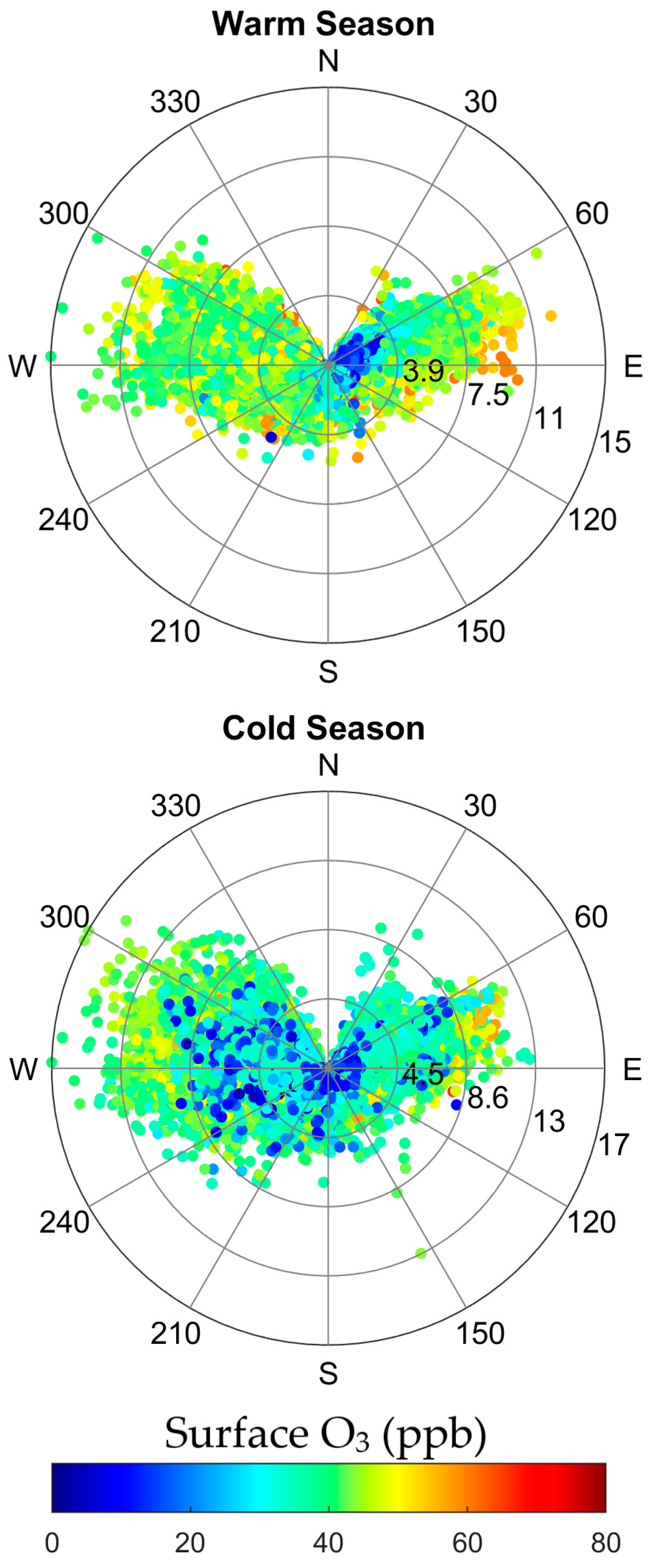
Figure 3.
Monthly variability of O3 (A, ppb), solar radiation (B, W/m2), and temperature (C, °C) at the LMT site. O3 data are differentiated per wind corridor.
Figure 3.
Monthly variability of O3 (A, ppb), solar radiation (B, W/m2), and temperature (C, °C) at the LMT site. O3 data are differentiated per wind corridor.
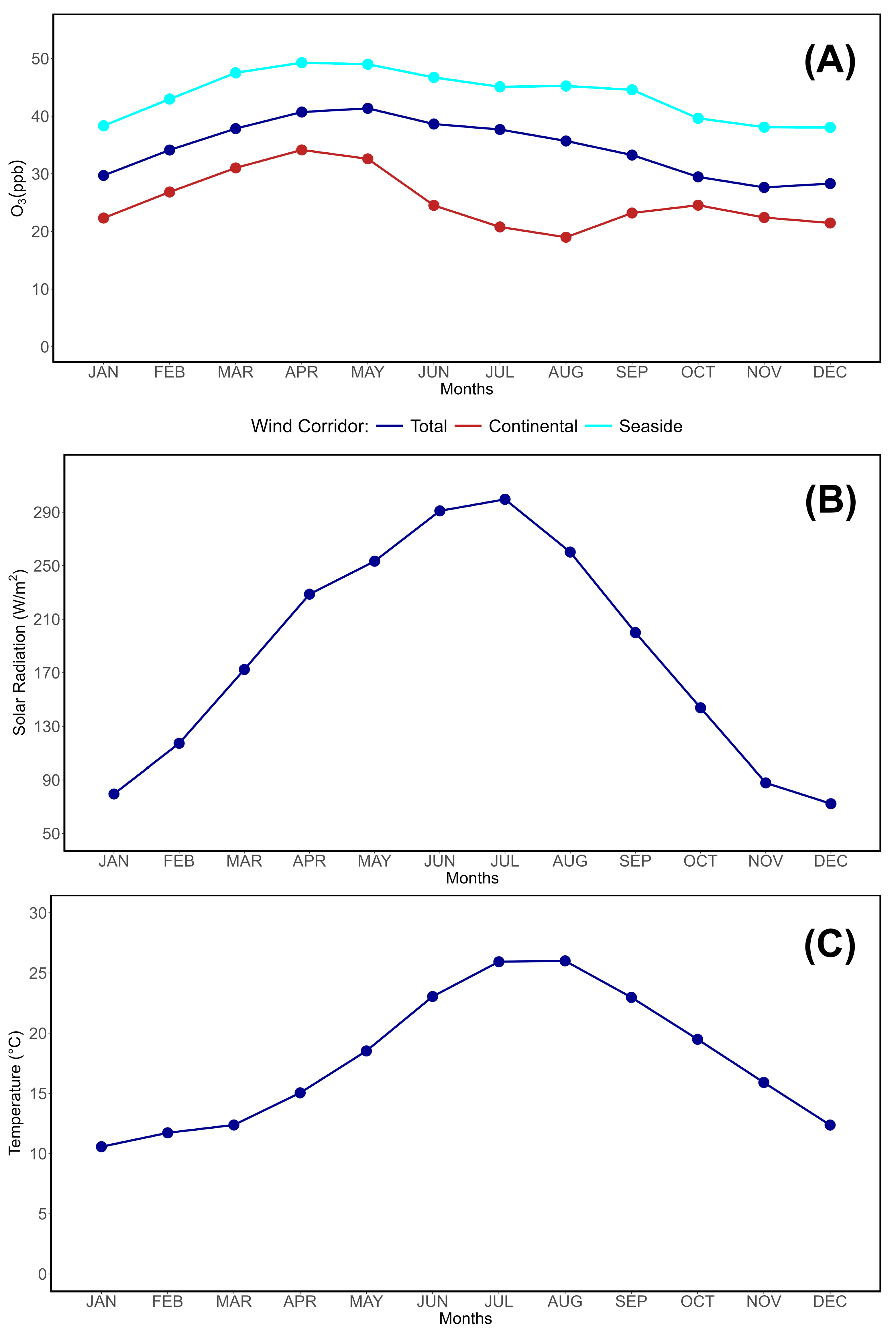
Figure 4.
Density distribution plots of O3 with solar radiation (A, W/m2) and temperature (B, °C). These plots consider all available data.
Figure 4.
Density distribution plots of O3 with solar radiation (A, W/m2) and temperature (B, °C). These plots consider all available data.
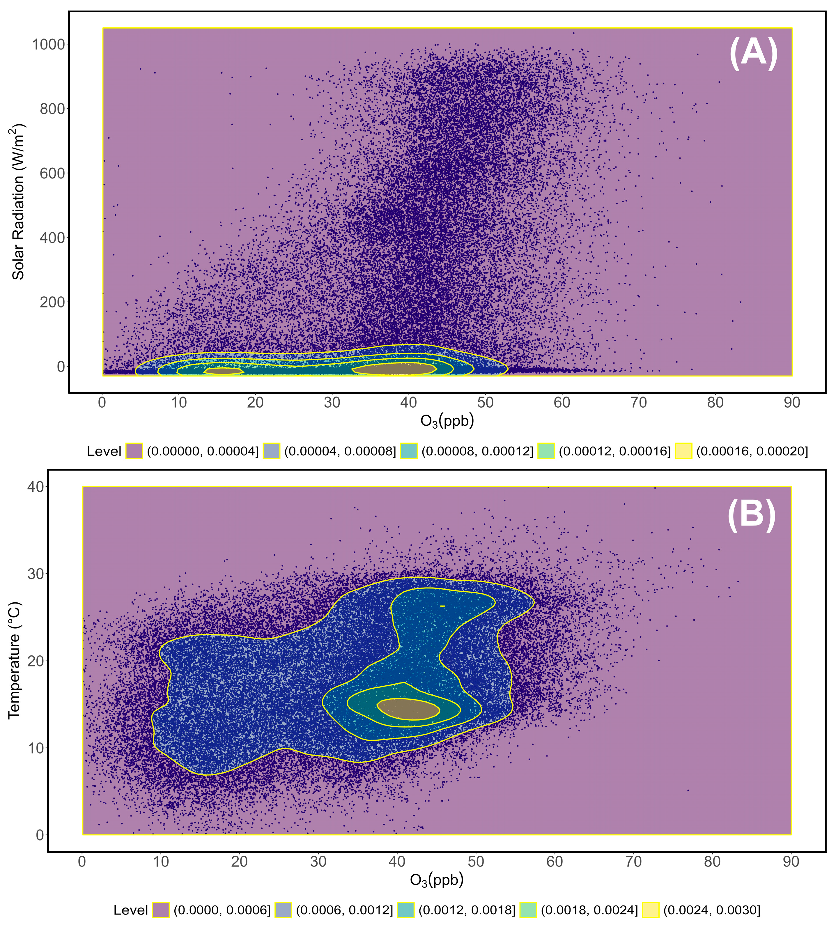
Figure 5.
Density distribution plots of O3 with solar radiation (A, W/m2) and temperature (B, °C). These plots consider the warm season (May-September) only.
Figure 5.
Density distribution plots of O3 with solar radiation (A, W/m2) and temperature (B, °C). These plots consider the warm season (May-September) only.
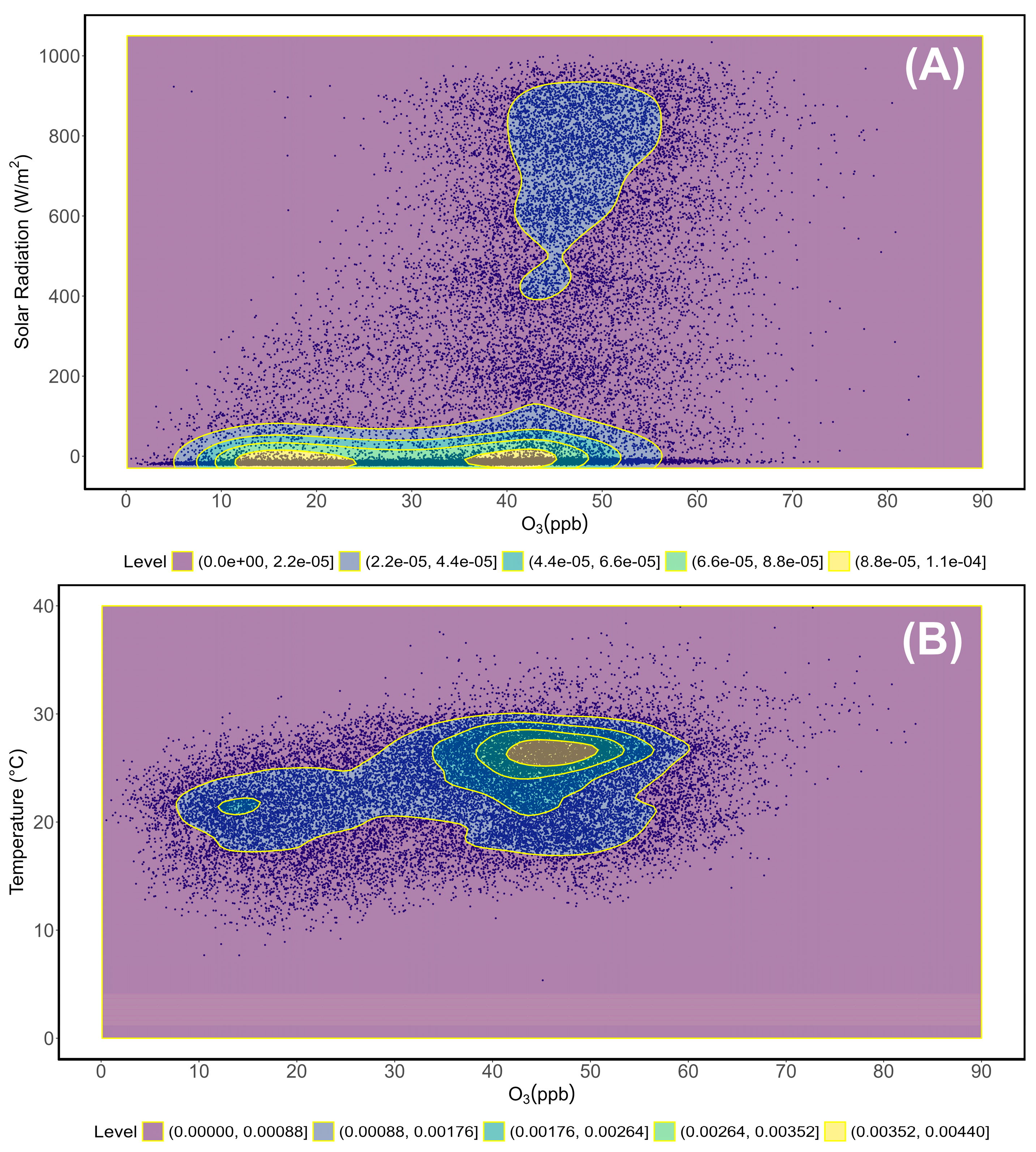
Figure 6.
Density distribution plots of O3 with solar radiation (A, W/m2) and temperature (B, °C). These plots consider the cold season (October-April) only.
Figure 6.
Density distribution plots of O3 with solar radiation (A, W/m2) and temperature (B, °C). These plots consider the cold season (October-April) only.
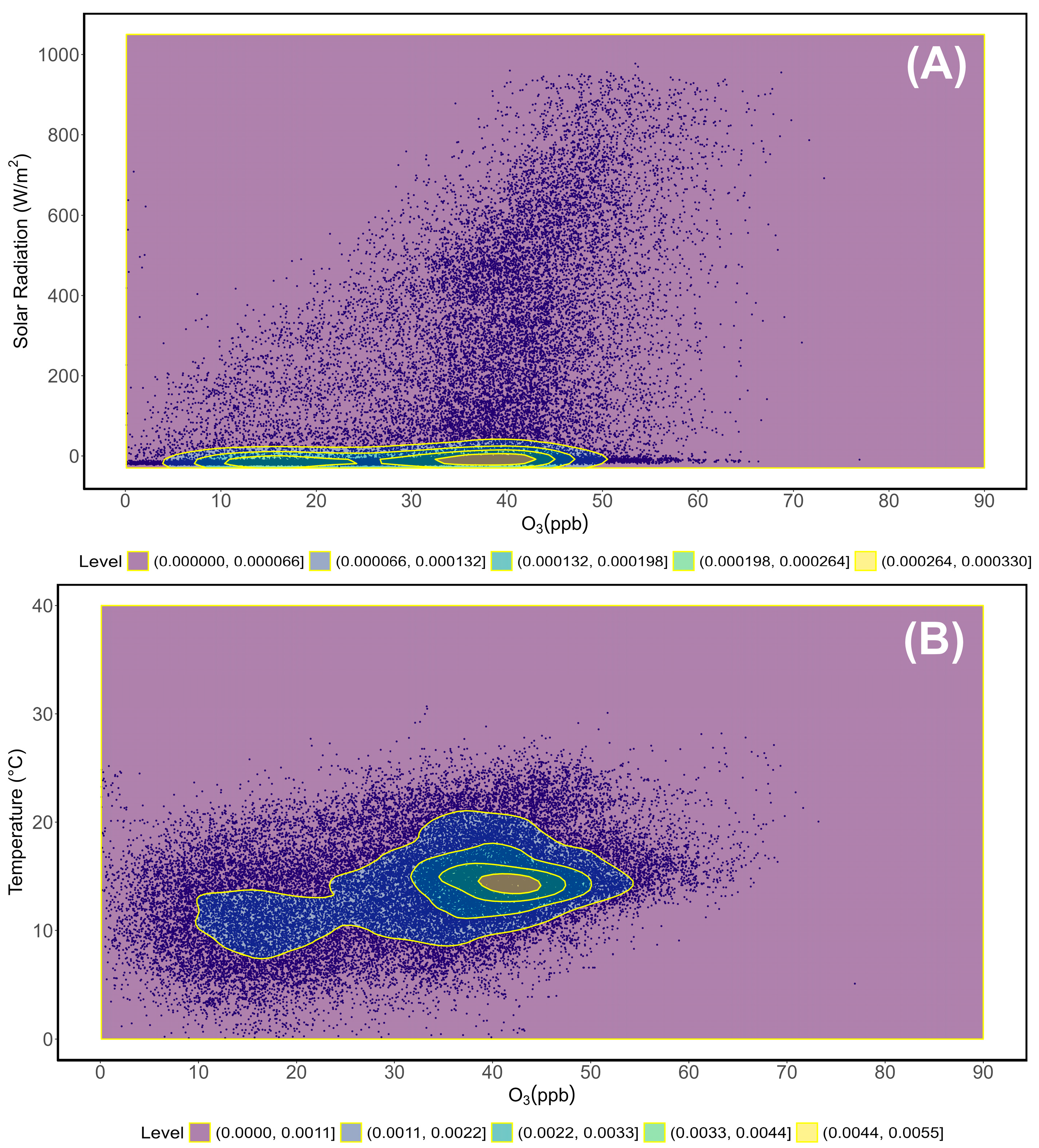
Figure 7.
Daily cycle of O3 (A, ppb), solar radiation (B, W/m2), and temperature (C, °C) differentiated by season. Shaded areas indicate intervals within one standard deviation (±1σ) from the average.
Figure 7.
Daily cycle of O3 (A, ppb), solar radiation (B, W/m2), and temperature (C, °C) differentiated by season. Shaded areas indicate intervals within one standard deviation (±1σ) from the average.
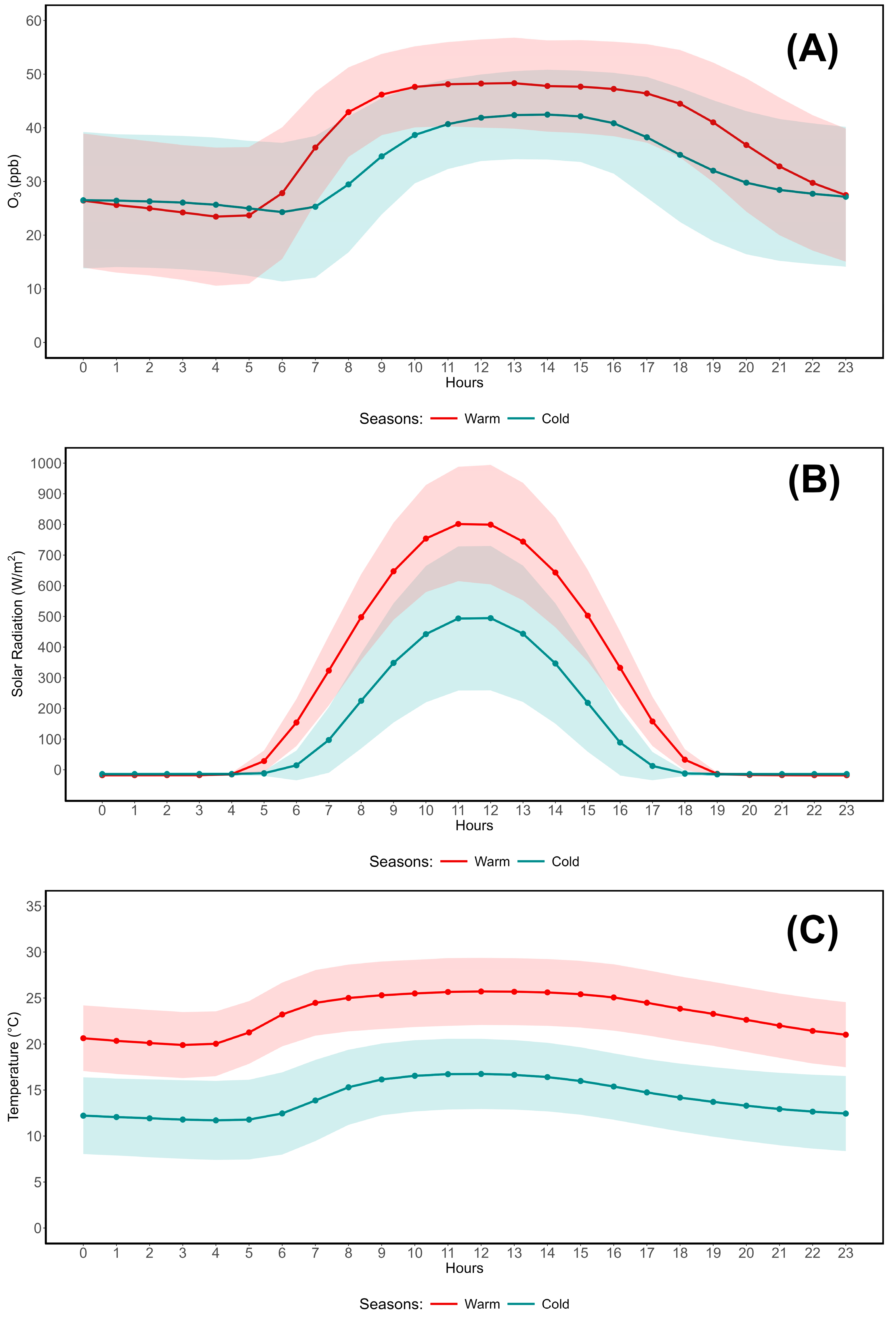
Figure 8.
Data ellipses following a normal distribution and an 80% confidence interval showing the variability of O3, during warm seasons, with solar radiation (A) and temperature (B).
Figure 8.
Data ellipses following a normal distribution and an 80% confidence interval showing the variability of O3, during warm seasons, with solar radiation (A) and temperature (B).
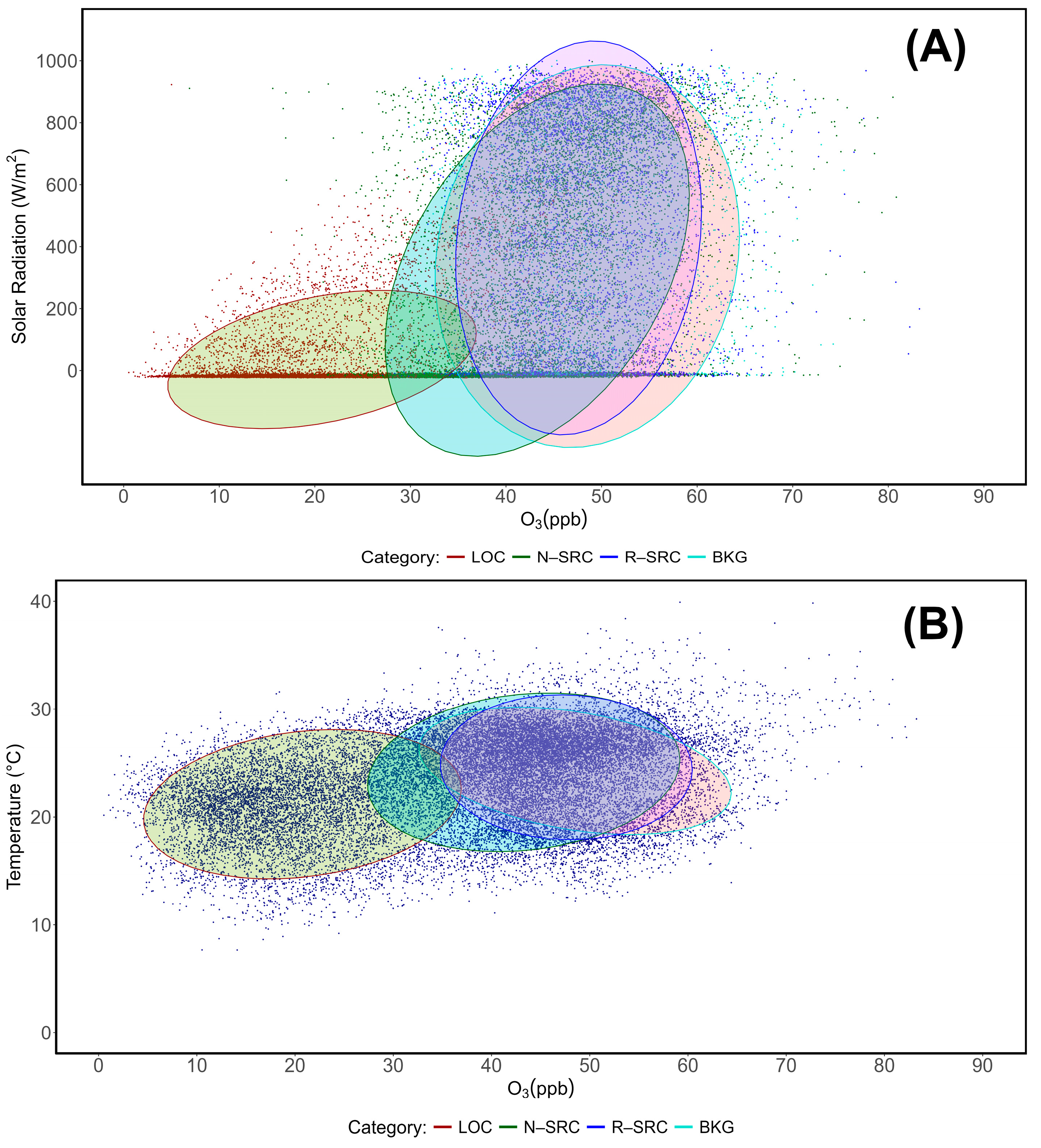
Figure 9.
Data ellipses following a normal distribution and an 80% confidence interval showing the variability of O3, during cold seasons, with solar radiation (A) and temperature (B).
Figure 9.
Data ellipses following a normal distribution and an 80% confidence interval showing the variability of O3, during cold seasons, with solar radiation (A) and temperature (B).
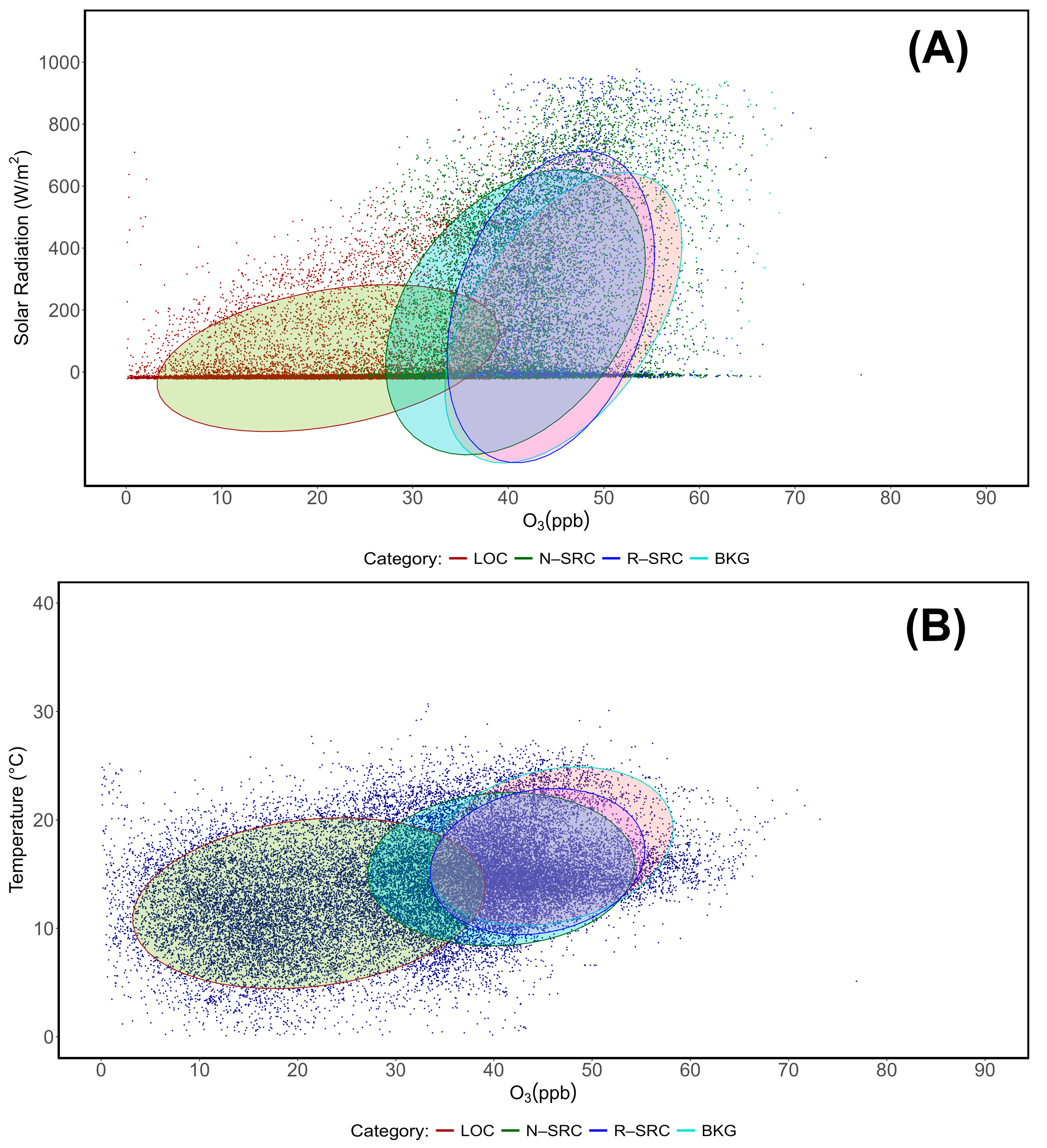
Figure 10.
Average O3 concentrations based on standard (LOC, N-SRC, R-SRC, BKG), corrected (R-SRCcor, BKGcor), and enhanced corrected (R-SRCecor, BKGecor) proximity categories. Shaded areas indicate intervals within one standard deviation (±1σ) from the average.
Figure 10.
Average O3 concentrations based on standard (LOC, N-SRC, R-SRC, BKG), corrected (R-SRCcor, BKGcor), and enhanced corrected (R-SRCecor, BKGecor) proximity categories. Shaded areas indicate intervals within one standard deviation (±1σ) from the average.
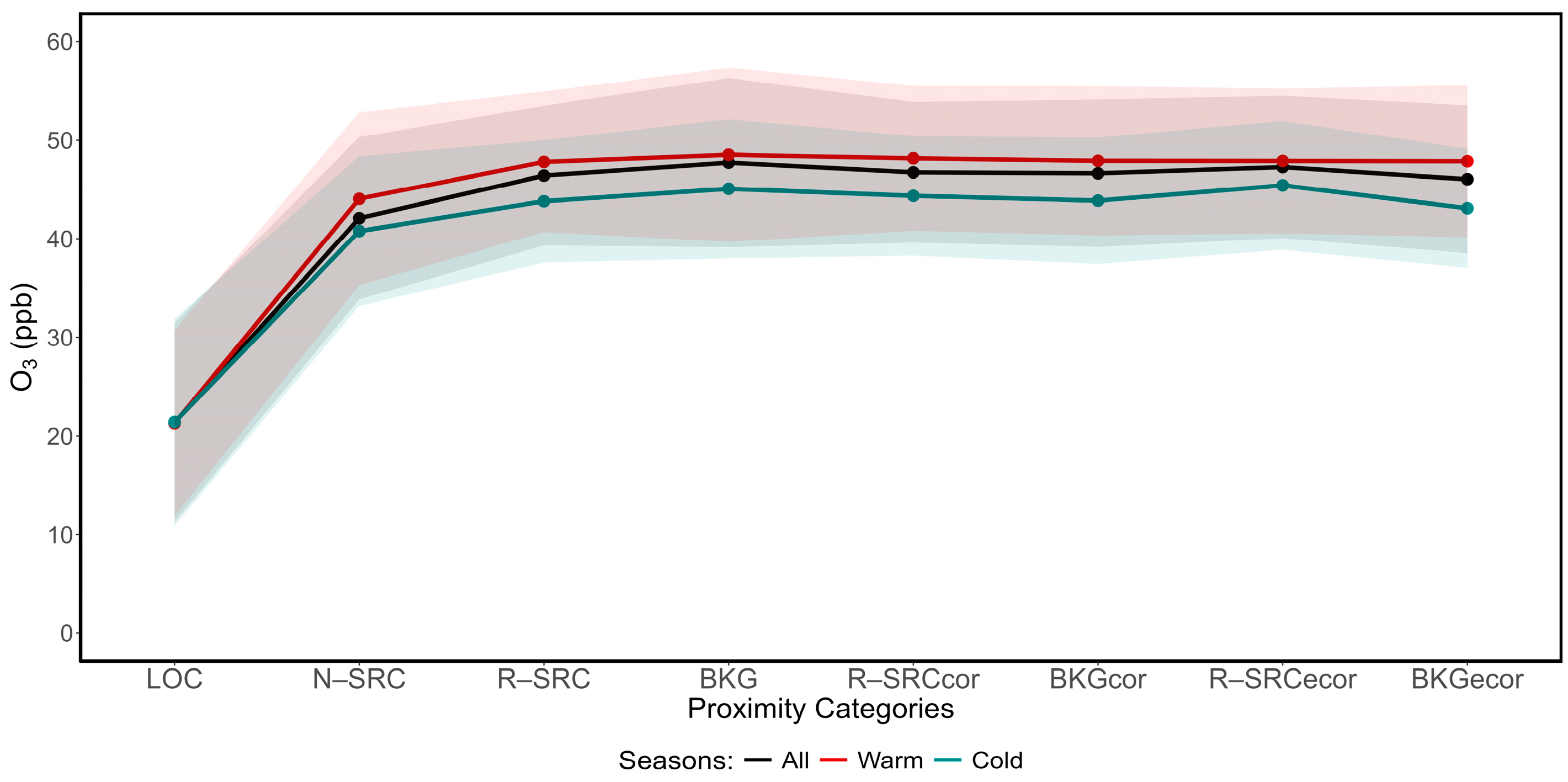
Figure 11.
Location of Stromboli and the “Ionian” point compared to the LMT observatory.
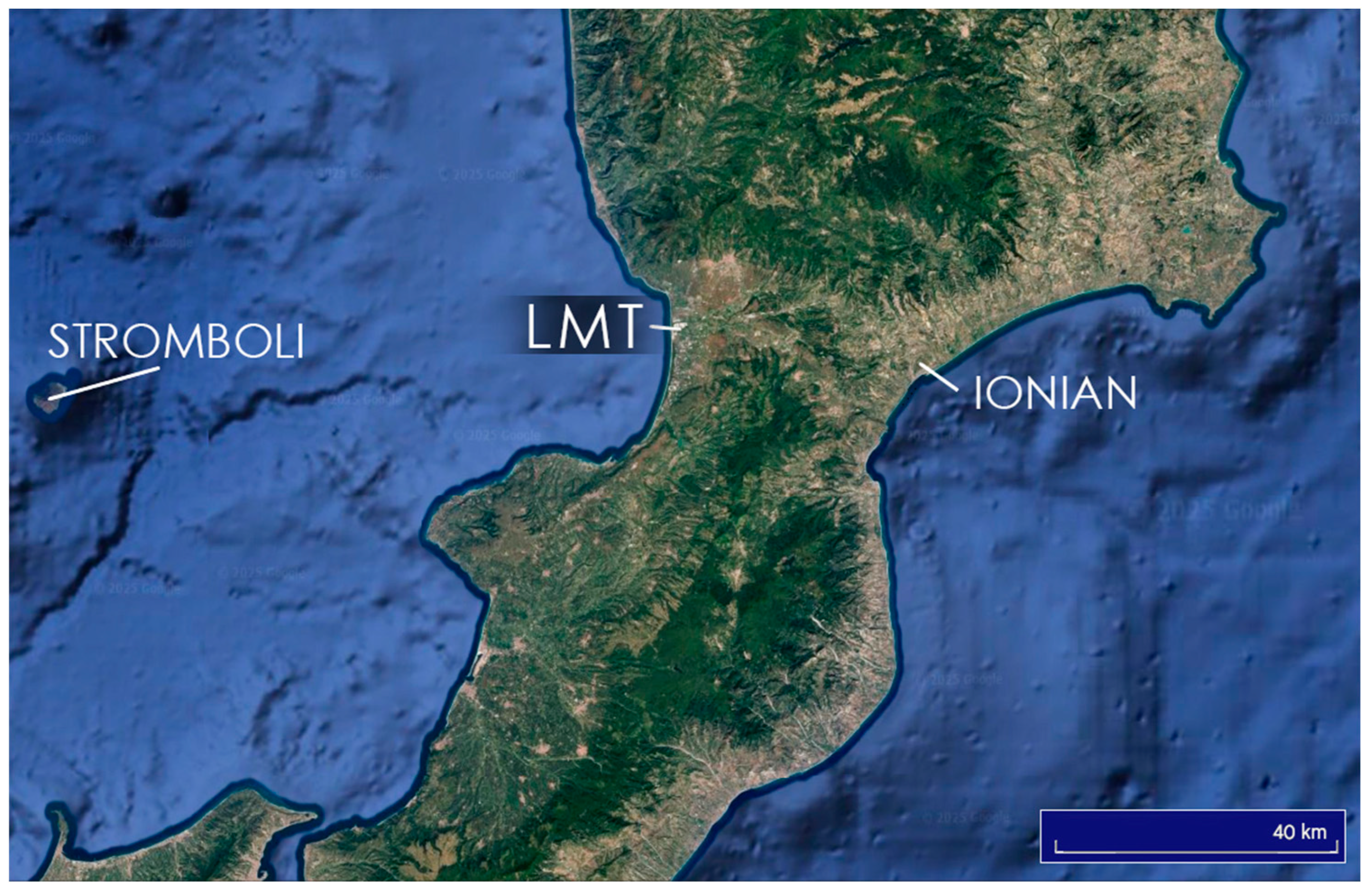
Figure 12.
Dual axis plots showing the variability of hourly O3 data with surface/DSSF solar radiation (A, W/m2), surface temperature (B, °C), and surface wind direction (C, °N).
Figure 12.
Dual axis plots showing the variability of hourly O3 data with surface/DSSF solar radiation (A, W/m2), surface temperature (B, °C), and surface wind direction (C, °N).
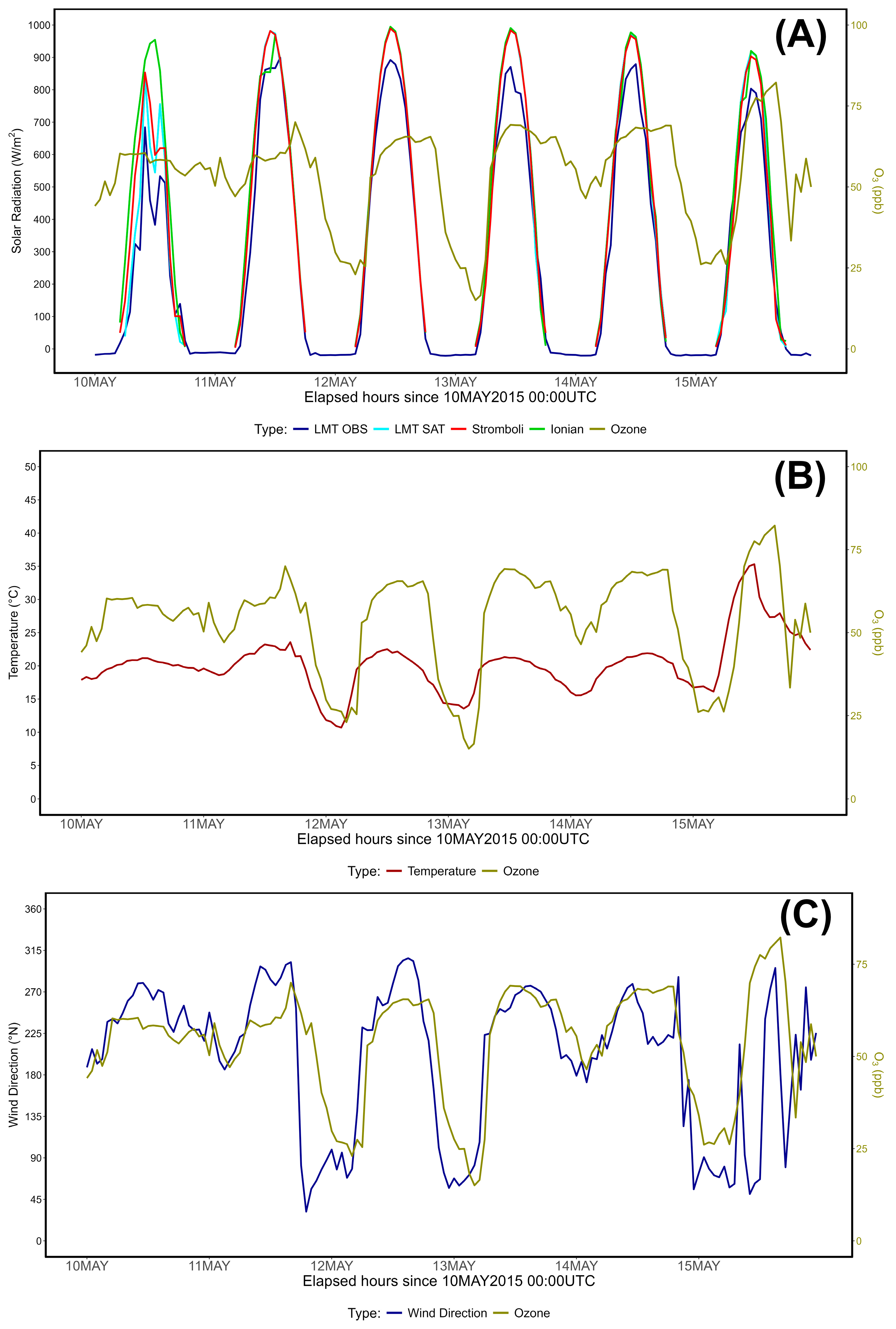
Figure 13.
OMI products showing available data concerning the evolution of the May 11th–15th , 2015 case study, also accounting for May 10th to assess the tropospheric distribution of O3 prior to the event. Data referring to May 11th were not available.
Figure 13.
OMI products showing available data concerning the evolution of the May 11th–15th , 2015 case study, also accounting for May 10th to assess the tropospheric distribution of O3 prior to the event. Data referring to May 11th were not available.
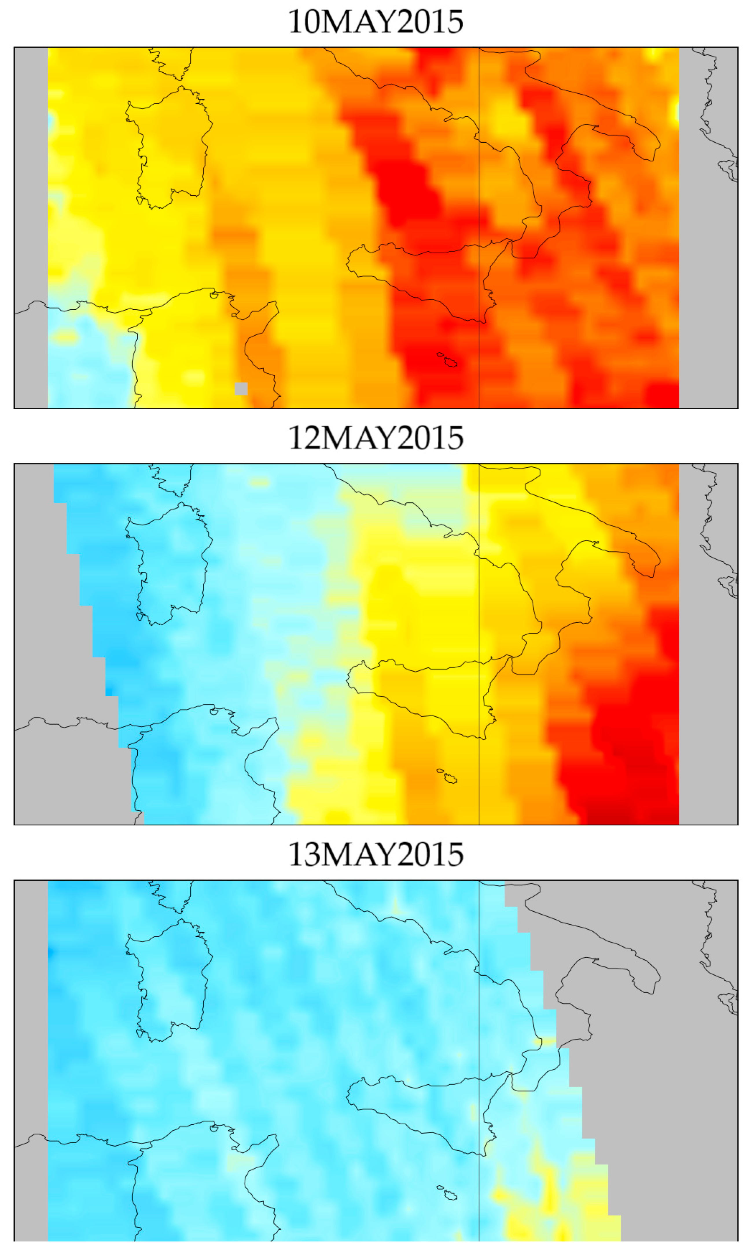
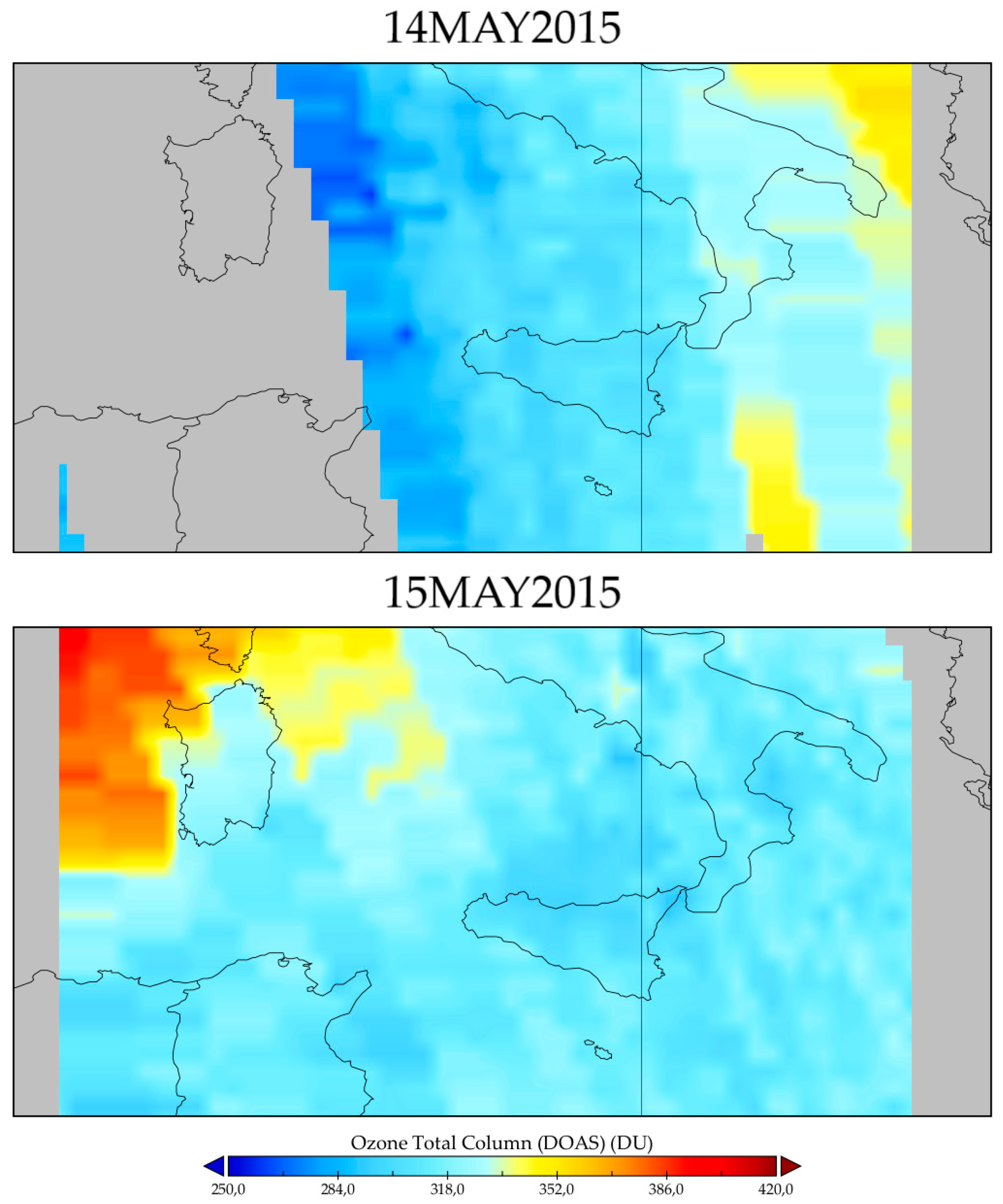

Table 1.
Coverage rates (%) of each dataset compared to the total number of elapsed hours. OZR refers to the dataset including valid ozone and radiation measurements. “Combined” refers to the dataset featuring valid measurements of all three instruments. Please note that 2016 and 2020 are both leap years, with extra 24 hours each.
| Year | Hours | Ozone | Radiation | Meteo | OZR | Combined |
|---|---|---|---|---|---|---|
| 2015 | 8760 | 92.13% | 99.62% | 95.90% | 91.76% | 90.15% |
| 2016 | 8784 | 96.17% | 98.58% | 96.35% | 95.15% | 93.03% |
| 2017 | 8760 | 95.94% | 96.97% | 93.80% | 93.07% | 91.29% |
| 2018 | 8760 | 98.13% | 25.15% | 77.05% | 24.04% | 24.01% |
| 2019 | 8760 | 94.19% | 98.57% | 98.60% | 94.16% | 94.13% |
| 2020 | 8784 | 98.51% | 100% | 99.99% | 98.51% | 98.50% |
| 2021 | 8760 | 91.16% | 99.91% | 99.75% | 91.16% | 90.99% |
| 2022 | 8760 | 85.23% | 99.95% | 90.11% | 85.23% | 81.99% |
| 2023 | 8760 | 81.95% | 85.97% | 96.30% | 68.69% | 67.35% |
| 78,8881 | 92.60%2 | 89.41%2 | 94.20%2 | 82.42%2 | 81.27%2 |
1 Total. 2 Average.
Table 2.
Correlation matrix showing the result of PCC (Pearson’s Correlation Coefficient) and SR (Spearman’s Rank) evaluations between O3 (ppb), solar radiation (W/m2), and temperature (°C). “All” columns refer to all available measurements of solar radiation at the site, while “Pos.” (positive) columns are restricted to measurements with positive SWdown values. “NE” refers to the northeastern sector of LMT (wind directions in the 0-90 °N range), while “W” refers to the western sector (240-300 °N). This table considers all data.
| Parameter | Statistics | Surface O3 (ppb) [All seasons] | |||||
| All Rad. | Pos. Rad. | All NE | All W | Pos. NE | Pos. W | ||
| Solar Radiation (W/m2) | df | 65023 | 31982 | 22806 | 24281 | 6139 | 18493 |
| PCC | 0.502 | 0.452 | 0.445 | 0.195 | 0.483 | 0.174 | |
| PCC p-value | < 0.001 | < 0.001 | < 0.001 | < 0.001 | < 0.001 | < 0.001 | |
| SR | 0.592 | 0.45 | 0.551 | 0.306 | 0.459 | 0.297 | |
| SR p-value | < 0.001 | < 0.001 | < 0.001 | < 0.001 | < 0.001 | < 0.001 | |
| Temperature (°C) | df | 70058 | 31664 | 24949 | 26410 | 6139 | 18493 |
| PCC | 0.362 | 0.268 | 0.256 | 0.096 | 0.273 | 0.071 | |
| PCC p-value | < 0.001 | < 0.001 | < 0.001 | < 0.001 | < 0.001 | < 0.001 | |
| SR | 0.352 | 0.259 | 0.22 | 0.149 | 0.243 | 0.106 | |
| SR p-value | < 0.001 | < 0.001 | < 0.001 | < 0.001 | < 0.001 | < 0.001 | |
Table 3.
Seasonal (warm) correlation matrix showing the result of PCC (Pearson’s Correlation Coefficient) and SR (Spearman’s Rank) evaluations between O3 (ppb), solar radiation (W/m2), and temperature (°C). “All” columns refer to all available measurements of solar radiation at the site, while “Pos.” (positive) columns are restricted to measurements with positive SWdown values. “NE” refers to the northeastern sector of LMT (wind directions in the 0-90 °N range), while “W” refers to the western sector (240-300 °N).
| Parameter | Statistics | Surface O3 (ppb) [Warm season] | |||||
| All Rad. | Pos. Rad. | All NE | All W | Pos. NE | Pos. W | ||
| Solar Radiation (W/m2) | df | 27773 | 15556 | 7111 | 12704 | 1684 | 10589 |
| PCC | 0.528 | 0.401 | 0.492 | 0.213 | 0.523 | 0.174 | |
| PCC p-value | < 0.001 | < 0.001 | < 0.001 | < 0.001 | < 0.001 | < 0.001 | |
| SR | 0.605 | 0.357 | 0.45 | 0.218 | 0.489 | 0.173 | |
| SR p-value | < 0.001 | < 0.001 | < 0.001 | < 0.001 | < 0.001 | < 0.001 | |
| Temperature (°C) | df | 29117 | 15408 | 7610 | 13431 | 1684 | 10589 |
| PCC | 0.343 | 0.103 | 0.265 | -0.098 | 0.251 | -0.111 | |
| PCC p-value | < 0.001 | < 0.001 | < 0.001 | < 0.001 | < 0.001 | < 0.001 | |
| SR | 0.316 | 0.041 | 0.169 | -0.115 | 0.19 | -0.132 | |
| SR p-value | < 0.001 | < 0.001 | < 0.001 | < 0.001 | < 0.001 | < 0.001 | |
Table 4.
Seasonal (cold) correlation matrix showing the result of PCC (Pearson’s Correlation Coefficient) and SR (Spearman’s Rank) evaluations between O3 (ppb), solar radiation (W/m2), and temperature (°C). “All” columns refer to all available measurements of solar radiation at the site, while “Pos.” (positive) columns are restricted to measurements with positive SWdown values. “NE” refers to the northeastern sector of LMT (wind directions in the 0-90 °N range), while “W” refers to the western sector (240-300 °N).
| Parameter | Statistics | Surface O3 (ppb) [Cold season] | |||||
| All Rad. | Pos. Rad. | All NE | All W | Pos. NE | Pos. W | ||
| Solar Radiation (W/m2) | df | 37248 | 16424 | 15668 | 11547 | 4448 | 7878 |
| PCC | 0.44 | 0.428 | 0.421 | 0.269 | 0.459 | 0.302 | |
| PCC p-value | < 0.001 | < 0.001 | < 0.001 | < 0.001 | < 0.001 | < 0.001 | |
| SR | 0.554 | 0.417 | 0.586 | 0.27 | 0.444 | 0.326 | |
| SR p-value | < 0.001 | < 0.001 | < 0.001 | < 0.001 | < 0.001 | < 0.001 | |
| Temperature (°C) | df | 40939 | 16254 | 17312 | 12948 | 4448 | 7878 |
| PCC | 0.355 | 0.166 | 0.402 | -0.033 | 0.338 | 0.209 | |
| PCC p-value | < 0.001 | < 0.001 | < 0.001 | < 0.001 | < 0.001 | < 0.001 | |
| SR | 0.351 | 0.147 | 0.397 | -0.001 | 0.315 | 0.229 | |
| SR p-value | < 0.001 | < 0.001 | < 0.001 | < 0.001 | < 0.001 | < 0.001 | |
Table 5.
Correlation matrix showing the results of PCC and SR evaluations of hourly O3 concentrations, temperature, and solar radiation based on the four main (LOC, local; N-SRC, near source; R-SRC, remote source; BKG, atmospheric background) proximity categories, as well as the corrected (“cor”) and enhanced corrected (“ecor”) categories of R-SRC and BKG..
| O3 by Cat. (ppb) | Statistics | Temp. (°C) |
Radiation (W/m2) |
|---|---|---|---|
| LOC | df | 27292 | 27292 |
| PCC | -0.057 | -0.008 | |
| PCC p-value | < 0.001 | 0.209 | |
| SR | 0.084 | 0.183 | |
| SR p-value | < 0.001 | < 0.001 | |
| N-SRC | df | 29183 | 29183 |
| PCC | -0.108 | 0.107 | |
| PCC p-value | < 0.001 | < 0.001 | |
| SR | 0.115 | 0.243 | |
| SR p-value | < 0.001 | < 0.001 | |
| R-SRC | df | 10852 | 10852 |
| PCC | -0.083 | 0.179 | |
| PCC p-value | < 0.001 | < 0.001 | |
| SR | 0.131 | 0.218 | |
| SR p-value | < 0.001 | < 0.001 | |
| BKG | df | 2536 | 2536 |
| PCC | -0.010 | 0.221 | |
| PCC p-value | 0.616 | < 0.001 | |
| SR | -0.130 | 0.210 | |
| SR p-value | < 0.001 | < 0.001 | |
| R-SRCcor | df | 2584 | 2584 |
| PCC | -0.077 | 0.147 | |
| PCC p-value | < 0.001 | < 0.001 | |
| SR | 0.153 | 0.224 | |
| SR p-value | < 0.001 | < 0.001 | |
| BKGcor | df | 10804 | 10804 |
| PCC | -0.061 | 0.197 | |
| PCC p-value | < 0.001 | < 0.001 | |
| SR | 0.078 | 0.216 | |
| SR p-value | < 0.001 | < 0.001 | |
| R-SRCecor | df | 4694 | 4694 |
| PCC | -0.042 | 0.131 | |
| PCC p-value | 0.004 | < 0.001 | |
| SR | 0.026 | 0.167 | |
| SR p-value | 0.070 | < 0.001 | |
| BKGecor | df | 7901 | 7901 |
| PCC | 0.093 | 0.188 | |
| PCC p-value | < 0.001 | < 0.001 | |
| SR | 0.110 | 0.195 | |
| SR p-value | < 0.001 | < 0.001 |
Table 6.
Correlation matrix of hourly O3 concentrations with temperature and radiation using PCC and SR statistics, differentiated by proximity category and wind sectors. These data refer to the warm season.
Table 6.
Correlation matrix of hourly O3 concentrations with temperature and radiation using PCC and SR statistics, differentiated by proximity category and wind sectors. These data refer to the warm season.
| O3 by Cat. (ppb) |
Statistics |
All Data | Northeast | West | |||
|---|---|---|---|---|---|---|---|
| Temp. (°C) |
Radiation (W/m2) | Temp. (°C) |
Radiation (W/m2) | Temp. (°C) |
Radiation (W/m2) | ||
| LOC | df | 10191 | 10191 | 5668 | 5668 | 437 | 437 |
| PCC | -0.118 | -0.032 | 0.108 | -0.020 | 0.041 | 0.173 | |
| PCC p-value | < 0.001 | 0.001 | < 0.001 | 0.135 | 0.397 | < 0.001 | |
| SR | 0.101 | 0.083 | 0.049 | 0.147 | 0.045 | 0.442 | |
| SR p-value | < 0.001 | < 0.001 | < 0.001 | < 0.001 | 0.343 | < 0.001 | |
| N-SRC | df | 11612 | 11612 | 1590 | 1590 | 5562 | 5562 |
| PCC | -0.107 | 0.024 | 0.303 | 0.024 | -0.057 | 0.027 | |
| PCC p-value | < 0.001 | 0.009 | < 0.001 | 0.340 | < 0.001 | 0.048 | |
| SR | 0.038 | 0.167 | 0.242 | 0.259 | -0.073 | 0.152 | |
| SR p-value | < 0.001 | < 0.001 | < 0.001 | < 0.001 | < 0.001 | < 0.001 | |
| R-SRC | df | 7084 | 7084 | 133 | 133 | 5398 | 5398 |
| PCC | -0.067 | 0.006 | 0.655 | 0.313 | -0.075 | 0.085 | |
| PCC p-value | < 0.001 | 0.590 | < 0.001 | < 0.001 | < 0.001 | < 0.001 | |
| SR | -0.078 | 0.072 | 0.654 | 0.357 | -0.087 | 0.119 | |
| SR p-value | < 0.001 | < 0.001 | < 0.001 | < 0.001 | < 0.001 | < 0.001 | |
| BKG | df | 1950 | 1950 | 22 | 22 | 1628 | 1628 |
| PCC | -0.011 | 0.089 | 0.344 | -0.102 | -0.329 | 0.154 | |
| PCC p-value | 0.629 | < 0.001 | 0.1 | 0.635 | < 0.001 | < 0.001 | |
| SR | -0.354 | 0.100 | 0.608 | 0.120 | -0.334 | 0.159 | |
| SR p-value | < 0.001 | < 0.001 | 0.002 | 0.575 | < 0.001 | < 0.001 | |
| R-SRCcor | df | 1617 | 1617 | 41 | 41 | 1192 | 1192 |
| PCC | -0.059 | 0.005 | 0.744 | 0.340 | -0.031 | 0.068 | |
| PCC p-value | 0.018 | 0.830 | < 0.001 | 0.026 | 0.277 | 0.02 | |
| SR | -0.022 | 0.082 | 0.769 | 0.479 | -0.06 | 0.12 | |
| SR p-value | 0.381 | < 0.001 | < 0.001 | < 0.001 | 0.038 | < 0.001 | |
| BKGcor | df | 7417 | 7417 | 114 | 114 | 5834 | 5834 |
| PCC | -0.049 | 0.028 | 0.587 | 0.237 | -0.161 | 0.106 | |
| PCC p-value | < 0.001 | 0.015 | < 0.001 | 0.010 | < 0.001 | < 0.001 | |
| SR | 0.166 | 0.075 | 0.610 | 0.200 | -0.17 | 0.129 | |
| SR p-value | < 0.001 | < 0.001 | < 0.001 | 0.031 | < 0.001 | < 0.001 | |
| R-SRCecor | df | 3515 | 3515 | 41 | 41 | 3089 | 3089 |
| PCC | -0.049 | -0.004 | 0.744 | 0.340 | -0.131 | 0.037 | |
| PCC p-value | 0.004 | 0.793 | < 0.001 | 0.026 | < 0.001 | 0.041 | |
| SR | -0.121 | 0.047 | 0.769 | 0.479 | -0.151 | 0.064 | |
| SR p-value | < 0.001 | 0.005 | < 0.001 | 0.001 | < 0.001 | < 0.001 | |
| BKGecor | df | 4876 | 4876 | 114 | 114 | 3294 | 3294 |
| PCC | -0.062 | 0.038 | 0.587 | 0.237 | -0.182 | 0.15 | |
| PCC p-value | < 0.001 | 0.007 | < 0.001 | 0.010 | < 0.001 | < 0.001 | |
| SR | -0.179 | 0.100 | 0.610 | 0.200 | -0.192 | 0.181 | |
| SR p-value | < 0.001 | < 0.001 | < 0.001 | 0.031 | < 0.001 | < 0.001 | |
Table 7.
Correlation matrix of hourly O3 concentrations with temperature and radiation using PCC and SR statistics, differentiated by proximity category and wind sectors. These data refer to the cold season.
Table 7.
Correlation matrix of hourly O3 concentrations with temperature and radiation using PCC and SR statistics, differentiated by proximity category and wind sectors. These data refer to the cold season.
| O3 by Cat. (ppb) |
Statistics |
All Data | Northeast | West | |||
|---|---|---|---|---|---|---|---|
| Temp. (°C) |
Radiation (W/m2) | Temp. (°C) |
Radiation (W/m2) | Temp. (°C) |
Radiation (W/m2) | ||
| LOC | df | 17099 | 17099 | 10892 | 10892 | 14238 | 14238 |
| PCC | 0.022 | 0.006 | 0.234 | -0.016 | 0.027 | 0.077 | |
| PCC p-value | 0.004 | 0.439 | < 0.001 | 0.088 | 0.001 | < 0.001 | |
| SR | 0.189 | 0.244 | 0.195 | 0.315 | -0.005 | 0.158 | |
| SR p-value | < 0.001 | < 0.001 | < 0.001 | < 0.001 | 0.555 | < 0.001 | |
| N-SRC | df | 17569 | 17569 | 5272 | 5272 | 7793 | 7793 |
| PCC | -0.015 | 0.181 | 0.163 | 0.124 | -0.11 | 0.167 | |
| PCC p-value | 0.051 | < 0.001 | < 0.001 | < 0.001 | < 0.001 | < 0.001 | |
| SR | 0.034 | 0.292 | 0.123 | 0.331 | -0.11 | 0.231 | |
| SR p-value | < 0.001 | < 0.001 | < 0.001 | < 0.001 | < 0.001 | < 0.001 | |
| R-SRC | df | 3766 | 3766 | 522 | 522 | 2564 | 2564 |
| PCC | -0.020 | 0.361 | 0.284 | 0.586 | 0.113 | 0.215 | |
| PCC p-value | 0.220 | < 0.001 | < 0.001 | < 0.001 | < 0.001 | < 0.001 | |
| SR | 0.116 | 0.359 | 0.317 | 0.577 | 0.104 | 0.227 | |
| SR p-value | < 0.001 | < 0.001 | < 0.001 | < 0.001 | < 0.001 | < 0.001 | |
| BKG | df | 584 | 584 | 83 | 83 | 539 | 539 |
| PCC | 0.007 | 0.556 | 0.635 | 0.467 | 0.190 | 0.563 | |
| PCC p-value | 0.866 | < 0.001 | < 0.001 | < 0.001 | < 0.001 | < 0.001 | |
| SR | 0.207 | 0.508 | 0.693 | 0.481 | 0.211 | 0.527 | |
| SR p-value | < 0.001 | < 0.001 | < 0.001 | < 0.001 | < 0.001 | < 0.001 | |
| R-SRCcor | df | 965 | 965 | 110 | 110 | 699 | 699 |
| PCC | 0.013 | 0.299 | 0.212 | 0.573 | 0.136 | 0.219 | |
| PCC p-value | 0.695 | < 0.001 | 0.025 | < 0.001 | < 0.001 | < 0.001 | |
| SR | 0.131 | 0.315 | 0.213 | 0.595 | 0.131 | 0.252 | |
| SR p-value | < 0.001 | < 0.001 | 0.024 | < 0.001 | < 0.001 | < 0.001 | |
| BKGcor | df | 3385 | 3385 | 495 | 495 | 2256 | 2256 |
| PCC | -0.022 | 0.409 | 0.337 | 0.571 | 0.126 | 0.262 | |
| PCC p-value | 0.194 | < 0.001 | < 0.001 | < 0.001 | < 0.001 | < 0.001 | |
| SR | 0.143 | 0.398 | 0.406 | 0.561 | 0.131 | 0.257 | |
| SR p-value | < 0.001 | < 0.001 | < 0.001 | < 0.001 | < 0.001 | < 0.001 | |
| R-SRCecor | df | 1177 | 1177 | 110 | 110 | 911 | 911 |
| PCC | 0.033 | 0.371 | 0.212 | 0.573 | 0.147 | 0.306 | |
| PCC p-value | 0.255 | < 0.001 | 0.025 | < 0.001 | < 0.001 | < 0.001 | |
| SR | 0.152 | 0.404 | 0.213 | 0.595 | 0.147 | 0.353 | |
| SR p-value | < 0.001 | < 0.001 | 0.024 | < 0.001 | < 0.001 | < 0.001 | |
| BKGecor | df | 3023 | 3023 | 495 | 495 | 1894 | 1894 |
| PCC | -0.044 | 0.353 | 0.337 | 0.571 | 0.138 | 0.145 | |
| PCC p-value | 0.015 | < 0.001 | < 0.001 | < 0.001 | < 0.001 | < 0.001 | |
| SR | 0.138 | 0.325 | 0.406 | 0.561 | 0.138 | 0.107 | |
| SR p-value | < 0.001 | < 0.001 | < 0.001 | < 0.001 | < 0.001 | < 0.001 | |
Table 8.
Average O3 concentrations and their respective standard deviations calculated on a per-category basis, and differentiated by season.
Table 8.
Average O3 concentrations and their respective standard deviations calculated on a per-category basis, and differentiated by season.
| Category | Average surface O3 (ppb) ± 1σ | ||
| All data | Warm season | Cold season | |
| LOC | 21.35 ± 10.11 | 21.28 ± 9.42 | 21.39 ± 10.50 |
| N-SRC | 42.08 ± 8.24 | 44.05 ± 8.76 | 40.77 ± 7.59 |
| R-SRC | 46.42 ± 7.08 | 47.81 ± 7.13 | 43.80 ± 6.20 |
| BKG | 47.73 ± 8.58 | 48.52 ± 8.84 | 45.07 ± 7.06 |
| R-SRCcor | 46.74 ± 7.13 | 48.17 ± 7.34 | 44.35 ± 6.05 |
| BKGcor | 46.64 ± 7.47 | 47.91 ± 7.58 | 43.86 ± 6.41 |
| R-SRCecor | 47.27 ± 7.22 | 47.90 ± 7.34 | 45.42 ± 6.53 |
| BKGecor | 46.04 ± 7.49 | 47.87 ± 7.72 | 43.09 ± 6.03 |
Table 9.
Correlation of hourly surface O3 with parameters measured at the LMT site (temperature, solar radiation – LMT OBS), and DSSF products (LMT SAT, Stromboli, Ionian).
Table 9.
Correlation of hourly surface O3 with parameters measured at the LMT site (temperature, solar radiation – LMT OBS), and DSSF products (LMT SAT, Stromboli, Ionian).
|
Statistics |
CS parameters | |||||
| LMT SAT (W/m2) | LMT OBS (W/m2) | Temp. (°C) |
Stromboli (W/m2) | Ionian (W/m2) | ||
| Surface O3 (ppb) | df | 86 | 142 | 142 | 87 | 87 |
| PCC | 0.456 | 0.51 | 0.617 | 0.463 | 0.464 | |
| PCC p-value | < 0.001 | < 0.001 | < 0.001 | < 0.001 | < 0.001 | |
| SR | 0.442 | 0.65 | 0.65 | 0.437 | 0.412 | |
| SR p-value | < 0.001 | < 0.001 | < 0.001 | < 0.001 | < 0.001 | |
Disclaimer/Publisher’s Note: The statements, opinions and data contained in all publications are solely those of the individual author(s) and contributor(s) and not of MDPI and/or the editor(s). MDPI and/or the editor(s) disclaim responsibility for any injury to people or property resulting from any ideas, methods, instructions or products referred to in the content. |
© 2025 by the authors. Licensee MDPI, Basel, Switzerland. This article is an open access article distributed under the terms and conditions of the Creative Commons Attribution (CC BY) license (http://creativecommons.org/licenses/by/4.0/).
Copyright: This open access article is published under a Creative Commons CC BY 4.0 license, which permit the free download, distribution, and reuse, provided that the author and preprint are cited in any reuse.


