
Submitted:
21 January 2025
Posted:
27 January 2025
You are already at the latest version
Abstract
Tree stems in both wetland and upland forests are a potentially significant source of the greenhouse gas methane (CH4). Stem CH4 emissions are assumed to play an important role on a global scale. Yet, uncertainties regarding temporal and spatial variability as well as transport processes of stem emissions remain high. Here, we assess the spatial variability and range of CH4 egress from 28 black alder (Alnus glutinosa) (L.) Gaertn.) trees based on data we recorded during three measurement campaigns in a mature alder carr in spring 2019. Fluxes varied significantly in time and space. The overall temporal variability during the three campaigns was larger than the spatial variability. The fluxes ranged from less than 1 µg m-2 h\textsuperscript{-1} to 450 µg m-2 h-1 with an average overall flux of 25 ± 59 µg m-2 h-1 (± SD). Stem CH4 fluxes were highest (61.6 ± 104.5 µg m-2 h-1) during higher soil temperatures in spring, with increasing sap flux density and an intermediate water level just above the surface (+2.7 ± 0.3 cm). Morphological properties of the trees, including diameter at breast height, their position on hummocks or hollows and height of the measurement on the stem, largely failed to explain variability in stem CH4 fluxes. Large scale topography (overall elevation gradient) within the study site and CO2 flux were the best predictors of stem CH4 emissions, but inundation and leaf out also significantly influenced stem CH4 fluxes. Thus, large scale factors such as topography as an indirect indicator for water level can potentially facilitate upscaling of tree stem CH4 emissions.
Keywords:
methane
; peatlands
; Black alder
; Alnus glutinosa
; stem
; tree
; temperate
; CH4
; emission
Highlights
- Stem CH4 fluxes show large variability within a small spatial range
- Stem CH4 fluxes respond quickly to changing environmental conditions
- Stem CH4 fluxes show time-consistent spatial patterns which are strongly associated with large scale topographic elevation
1. Introduction
Methane (CH4) emissions from tree stems have been commonly observed in forested wetlands [1,2,3,4] and upland forests [5,6]. Still, the magnitude of stem CH4 emissions are considered to be a major knowledge gap in the global carbon cycle [7]. Relative to soil emissions, stem emissions have been reported to be either of low importance [8] or of intermediate or even high importance in ecosystem CH4 budgets [3,9,10]. Very high variability has been found in stem CH4 emissions, both seasonally [3,8] as well as spatially [11]. The spatial variability is thought to be coupled to water table depth [11], which ultimately depends on the topography of the studied site. Most often, an increase in stem CH4 emissions has been found to be associated with increasing water tables [3,4,5,12,13]. More precisely, peaks of stem CH4 emissions were associated with water tables just above the soil surface, and a further increase in water levels did not increase CH4 fluxes [3]. Increasing temperatures are another important factor that can explain rising stem CH4 fluxes [7,13,14]. Generally, studies of stem CH4 fluxes have shown high variability which can also partly be explained from different measurement settings. Upland forests often show low fluxes and low contributions to overall CH4 emissions [9,15] while very high fluxes with very high contributions to the overall ecosystem CH4 budgets have repeatedly been reported from tropical and/or systems with water-logged or permanently wet soils [10,16].
Two most likely origins of the emitted CH4 are discussed in the literature: 1) production in the soil and subsequent uptake by the roots and transport within the tree, either actively in the sap or passively by diffusion in air-filled spaces. This theory is supported by several studies reporting the highest emissions of the relevant gases from the lowest parts of the trees [7,8,10,16,17,18]. Thus, the topographic location of the tree itself may influence stem CH4 emissions (i.e., trees located at lower elevation are more often connected to the anoxic layer in the soil resulting in higher stem CH4 emissions). 2) Production within the stem and subsequent radial diffusion to the atmosphere: Here, heartwood rot is thought to be a possible driver of stem CH4 emissions [19,20] which will, however, not be considered further in this study as neither wood samples nor microbiology samples were taken and the focus lies on rather large scale variability.
Regardless of the origin of the CH4, transport mechanisms inside the tree play an important role and are themselves strongly dependent on the abiotic and biotic environment. CH4 from the soil can be transported solely by diffusion, which is indicated by decreasing CH4 emissions with increasing stem height [16]. Further, pressurized ventilation can cause variable CH4 emissions in time, due to changes in air and surface temperature of the plant which in turn are caused by increasing solar irradiation [21]. Also, CH4 transport through the xylem can be driven by transpiration, thus increased transpiration during higher temperatures is likely to increase CH4 emissions from plants [9,22], which however is species dependent [9].
The spatial and temporal variability of CH4 emitted from tree stems adds uncertainties when upscaling CH4 emissions. Here, we address the temporal and spatial patterns of stem emissions in a temperate alder wetland. We include spatial factors such as the height of the measurement relative to the stem base, the relative orthometric height of the tree base in comparison to the overall topography and temporal factors such as the varying environmental conditions (i.e., water table fluctuations, air temperature and sap flow density). Thus, for our study we formulate the following hypotheses:
- General elevation (i.e., orthometric height of the tree base) explains, at least in part, the spatial variability of stem CH4 emissions.
- The effect of small scale topography (hummocks, hollows) plays a minor role compared to large scale topography (general elevation).
- Stem CH4 emissions increase with an increase in biological activity (i.e., sap flux in trees and soil temperature)
- The water level is the prime factor influencing the temporal variability of stem CH4 flux.
2. Materials and Methods
The study site, a temperate Black alder (Alnus glutinosa (L.)Gaertn.) forest with fluctuating water tables, is located in north-eastern Germany (54° 7’ 36.27” N, 12° 28’ 55.5” E; see Figure 1). The site was drained in the past and the trees were logged before the site was gradually rewetted in 1998, with the final water level establishing in 2004. The site is located at an elevation of approx. 40 m a.s.l. and is situated within a local depression. It is characterized by hummocks covered by trees and hollows that are inundated for a few months a year. The average annual precipitation and temperature are 627 mm and 8.5°C, respectively (derived from the 1 km grid product of the German Weather Service, [23], reference period: 1981–2010). Black alder (Alnus glutinosa) is the only tree species at the site while the understorey is dominated by sedges (Carex acutiformis Ehrh., Carex riparia Curtis), Featherfoil (Hottonia palustris L.) and Bitter nightshade (Solanum dulcamara L.). At the time of study the forest had a uniform age of approximately 40 years and the trees had an approximate stem height of 15-20 m. The diameter at breast height (DBH) was 34.6 ± 6.2 (SD) cm. For more details see [24].
2.1. Study Setup
Within the stand 28 trees were chosen that were located within a depression with high water table variability. Further, the trees were chosen based on their location on large, elevated hummocks (n = 10), smaller hummocks (n = 11) and trees that were not located on a hummock (n = 7). One chamber per tree was permanently installed with adhesive synthetic sealant (plastic fermit ©) at between 30 and 80 cm above the stem base, depending on feasibility due to the surface roughness of the bark. Yet the chambers were located as low on the stem as possible as we expected the highest fluxes in this height. These closed dynamic chambers (non-steady-state through-flow) [25,26] were constructed from polypropylene containers from which the bottom was cut out (V = 0.001 m³ EMSA ©). All 28 chambers were installed in early March 2019 and measurement campaigns were carried out on the 24th of April 2019, the 14th of May and the 28th of May 2019. The dates of the campaigns were chosen to cover the period in which Black alder leafs out suggesting an increase of the physiological activity of the trees and a change of environmental conditions.
2.2. Flux Measurements
To perform a measurement with a stem chamber, a lid with a rubber gasket was mounted on top of the chamber to make it gas tight. The chamber was connected to a GHG analyzer via PVC tubing. During chamber closure, we simultaneously measured CO2 and CH4 concentrations inside the chamber with laser-based gas analysers (either an Ultra portable Greenhouse Gas Analyzer (Los Gatos Research Inc) or a GasScouter (Picarro Inc.)) with measurement frequencies of 1 and 2 Hz, respectively. We used a closing time of 3 min because changes in gas concentrations inside the chambers were quickly visible in trial measurements. However, when concentration changes were slow, we prolonged the closure time up to 7 min. We estimated fluxes with the fluxx function of the package flux for R [27] and opted for median based regression to estimate the fluxes. Here, the slopes between concentration values are calculated in a moving window fashion and subsequently, the median of all slope values provides the slope to estimate the flux [28]. Fluxes are then derived by using the determined slope in the following equation:
with M the molar weight of CH4, p the atmospheric pressure [hPa], V the volume of the chamber [m3], R the gas constant (R = 0.0821), T the air temperature in Kelvin, A the base area of the chamber (stem area) and the change of CH4 concentration over time. All subsequent statistical analyses were carried out using R version 4.0.2 [29].
2.3. Environmental Variables
Soil temperatures were measured and logged automatically every 15 min at three locations in two depths (5 and 15 cm) (HOBO UA-001-64, Onset Computer Cooperation, MA. USA). A weather station located 500 m SE of the study site monitored air temperature, precipitation, relative humidity and photosynthetically active radiation (PPFD (photosynthetic photon flux density) in µmol m-2 s-1). Water level was monitored at an interval of 1 min at a central location in the stand using a SEBA © CS457 dipper connected to a CR300 logger (Campbell Scientific ©). Furthermore, we used a digital elevation model (DEM) with 1m horizontal and 0.25m vertical resolution (©GeoBasis-DE/M-V 2015) to derive the topographic wetness index (TWI) by calculating the slope and specific catchment area [30] with QGIS and SAGA [31]. The TWI is used to estimate lateral water transport and can, thus, be used as a predictor for water accumulation.
We assumed that the vertical position of the trees relative to the ground could be of high importance for the measured fluxes. However, the vertical resolution of the DEM was not accurate enough for this purpose. Therefore, we recorded the exact vertical positions (orthometric height) of all tree stem bases with a tachymeter at the site with a vertical precision of higher than 1 cm. Additionally, the diameter at breast height (DBH) and the height of the chamber location above the stem base was recorded (HASB). Moreover, the tachymeter measurements were used to measure the relative orthometric soil height at distinct points (n=24) between all trees monitored. This information was then used to interpolate the soil surface using IDW interpolation. For each tree a soil height value was then sampled from the interpolated raster.
In order to obtain interpolated water level values across the stand the difference between the orthometric height of the ground water well and the sampled points in the stand was calculated. On the base of the recorded ground water level (daily average of each campaign day) and the height difference between the ground water well and the sampled heights from the raster an interpolated water level could be calculated. This was used to add a categorical variable inundated that entered statistical analyses stating if the tree base was inundated or not. An additional categorical variable leaf.out stated if the measurement was taken prior or post leaf out.
Further, sap flux density was measured at three representative black alder trees with the heat field deformation method (HFD) with a pair of permanently installed thermocouples on each tree (Type SF-G, Ecomatik GmbH, Dachau, Germany). We calculated the sap flux density with the following formula by
with U the sap flux density in [ml m-2s-1], the maximum value of every day, and the temperature difference between the pair of thermocouples installed in the tree.
All data analyses and visualizations were done using R [29,32]. In order to test for significant differences of stem GHG exchange between measurement campaigns, the entire flux data set was tested for normality using Shapiro-Wilk test. As the flux data set was not normally distributed Wilcoxon-Mann-Whitney test was used to determine statistically significant differences between the campaigns.
Linear mixed effect models were used to find the variables having the strongest effect on stem CH4 fluxes. Prior to analyses using linear mixed effect models, all numerical variables were centered and scaled. The best performing model was chosen by manual backward selection, e.g., successively leaving out the variable with the lowest t-value. Subsequently, the conditional R2 was calculated using the performance package in R [33]. This procedure was done as long as R2 did not decrease. The final model incorporated the individual tree as a random effect and orthometric height, CO2 flux, TWI, leaf out, HASB and inundated as fixed effects. An ANOVA was carried out on the final model parameters in order to obtain levels of significance. Averages are given ± 1 standard deviation (SD).
3. Results
3.1. Environmental Parameters
Environmental parameters varied significantly over the course of the measurement period. Generally, air temperatures increased from the second campaign onward and precipitation was relatively low. During the week preceding each measurement campaign, average air temperatures were 10.8 °C, 8.8 °C and 12.6 °C, for campaign one, two and three, respectively. Total precipitation during the week preceding each campaign was 0.1 mm, 6.2 mm and 0.2 mm for campaign one, two and three, respectively.
Figure 2.
Air temperature recorded at the weather station close to the study site and precipitation data obtained from the DWD grid data
Figure 2.
Air temperature recorded at the weather station close to the study site and precipitation data obtained from the DWD grid data
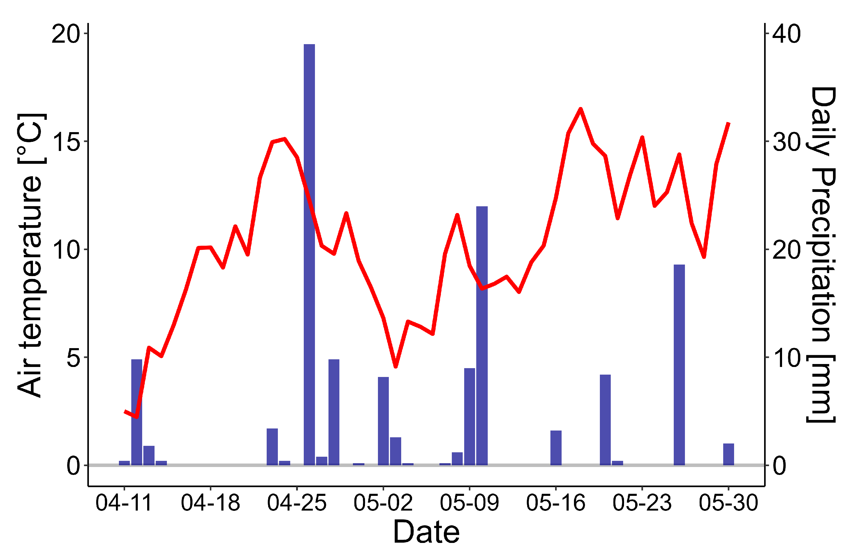
Water levels dropped from above the soil surface to below soil surface during the study period, overall averaging +4.5 ± 5.5 cm. Soil temperatures gradually increased and on average were 10.1 ± 2.3 °C and 9.6 ± 2.1 °C at 5 and 15 cm depth, respectively. The third campaign differed quite strongly from the first and second campaigns in that soil temperatures were approx. 3°C higher and water levels were lower (-5cm in contrast to water levels above ground surface during the first and second campaign).
Shortly after the second campaign and following leaf out, sap flux density increased strongly, indicating a strong increase in physiological activity (Figure 3). This was likely triggered by increasing air temperature and radiation (data not shown).
3.2. Tree Stem CH4 and CO2 Exchange
All tree stems that we monitored (n = 28) were at least temporarily a source of CH4 during the three campaigns and we did not measure noteworthy CH4 uptake (Figure 3). Generally, CH4 fluxes (n = 252) were low across the stand with few maxima. Fluxes varied significantly between campaigns (p = 0.02), averaging 16 ± 25 µg m-2 h-1 on April 24th, 64 ± 106 on May 14th and 15 ± 20 µg m-2 h-1 on May 28th. Highest fluxes of each campaign reached 83 µg m-2h-1, 452 µg m-2h-1 and 77 µg m-2h-1, respectively. Notably, six trees acted as high emitters showing much higher emissions than the majority of the other trees (Figure 4).
The tree stems acted as a source for CO2. CO2 fluxes also differed significantly during the campaigns (p = 0.01), however not as many outliers were apparent as were in the CH4 fluxes. Further, the magnitude of the CH4 fluxes was much lower than that of the CO2 fluxes. The overall mean stem CO2 flux was 57.1 ± 37.3 mg m-2h-1. The average CO2 fluxes by campaign were 53.8 ± 33.1 mg m-2 h-1, 49.4 ± 33.1 mg m-2 h-1 and 65.3 ± 44.4 mg m-2 h-1 for the campaigns one to three, respectively. The highest measured flux was 234.2 mg m-2h-1 on May 28th.
3.3. Topography
The range of the TWI (topographic wetness inde) within the stand was relatively small (3 to 8.9) compared to the overall dataset (0-27). Thus, the TWI may be limited in giving explanations regarding the topographic setting of the trees. The orthometric height that was measured within the site revealed variable microtopography with a minimum of 36.85 m and a maximum of 37.44 m above sea level.
3.4. Controlling Factors of Stem CH4 and CO2 Fluxes
Neither DBH (diameter at breast height) nor the vertical position of the tree base (hummock, hollow) significantly explained differences in stem CH4 flux, as did the soil temperature measured in the middle of the stand. The vertical position of the chamber (HASB = height above stem base) and CH4 fluxes were only significantly related for the first and last campaign (R2 = 0.25, p = 0.006 and R2 = 0.23, p = 0.009, respectively). When fluxes generally increased during the second campaign the relationship ceased (R2 = 0.11, p = 0.084). However, CO2 fluxes and CH4 fluxes were significantly positively related with each other on all measurement days (R2 = 0.19, p < 0.01). However, the strength of the relationship varied strongly between campaigns (campaign 1: R2 = 0.67, p < 0.01; campaign 2: R2 = 0.52, p < 0.01; campaign 3: R2 = 0.57, p < 0.01) and was caused by only very few fluxes (Figure 5).
In simple linear regression, the TWI showed no significant relationship with the CH4 flux. The orthometric height showed a weak, yet significant, overall negative relationship with CH4 emissions (R2 = 0.14, p < 0.001), which was strongest during the second measurement campaign (Figure 5) (R2 = 0.29, p < 0.01).
After manual backward selection of linear mixed effect models the final best performing model consisted of six variables. The factor of inundation had the strongest effect on stem CH4 fluxes (t = 3.8, p < 0.01) followed by CO2 flux (t = 3.6, p < 0.01), leaf out (t = -3.5, p < 0.01) and orthometric height (t = -2.1, p = 0.04).
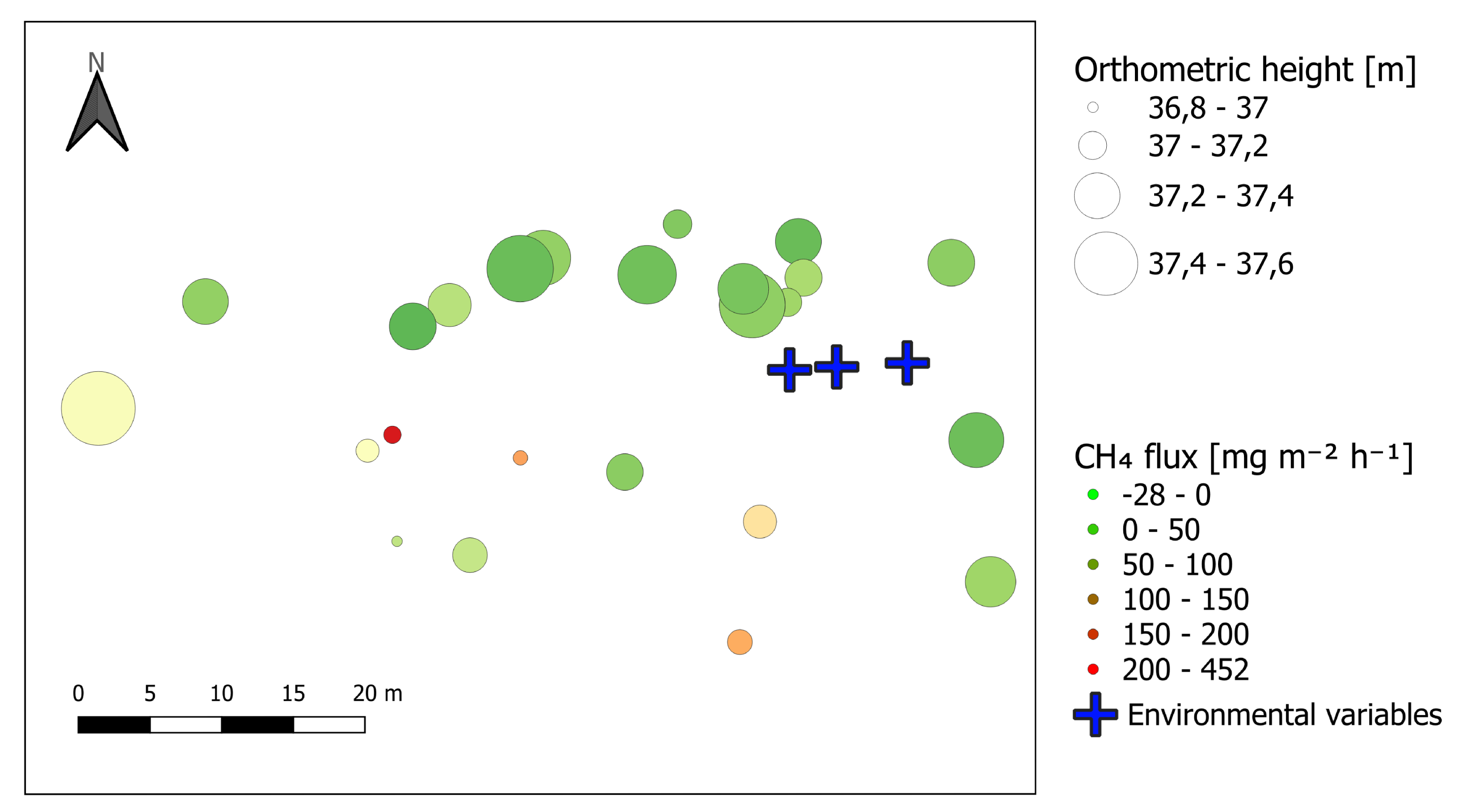
CH4 fluxes showed a distinct spatial pattern (Figure 6) with the southern half of the trees constantly showing higher CH4 fluxes than the trees of the northern half. Overall elevation seems to have had an effect on stem CH4 fluxes, as higher orthometric height was spatially associated with lower stem CH4 fluxes.
4. Discussion
In general, our results confirm that Black alder (Alnus glutinosa (L.) Gaertn.) stems can act as sources for CH4 emissions, as we have shown with long-term data from the site elsewhere [8]. Stem CH4 fluxes measured in this study were in the lower range of fluxes reported in other studies from temperate wetlands [8,18,34], but rather fall into the range of fluxes reported from upland forests [19,20]. The CH4 fluxes on the second measurement day with favourable conditions for CH4 production, however, were comparable to those from other wet temperate alder [34] and dry upland beech forests [35].
4.1. Spatial Variation of CH4 Fluxes
CH4 emissions from the 28 measured trees showed considerable spatial variability. Moreover, this variation was stable over time, with the same trees showing the highest emissions on all days. This suggests that either physiological/morphological traits, or abiotic factors such as temperature or water level in proximity of the tree influence CH4 formation and emission. Topographic position of trees has been shown to be a good indicator of stem CH4 emissions [5,18]. This is not surprising since water level is an important driver of CH4 production [2,12,14,17]. Water level differences of 20 cm can make a large difference for CH4 production and oxidation [36], which lies in the typical range of height differences a hummock can make, suggesting lower CH4 production and emissions from alder trees on hummocks. On the other hand, hummocks, protruding slightly out of the water, can also have much higher soil temperatures in spring than the low-lying, water-covered areas. This in turn can increase production of CH4 since methanogenesis is, like all microbial processes, strongly temperature dependent [37,38,39]. Against this background, it is quite astonishing that neither the topographic wetness index nor the categorical position variable (high hummock, low hummock, no hummock) was significantly related with stem CH4 fluxes in our data set.
One reason for this might be the fact that there is a slight elevation gradient across the site. Although the 28 trees are all situated in a depression, the southern part of the study area is located a bit lower than the northern half, which potentially leads to a longer duration of inundation. Indeed, CH4 emissions from trees in the southern half of the study area were generally higher throughout the measurement campaigns. This indicates that the large-scale topographic position of the trees is of importance and can function as a proxy for the relative water table position. This explanation is further supported by the fact that the interpolated water level was the variable having the strongest effect on stem CH4 fluxes. The fact that the calculation of the Terrain Wetness Index did not yield satisfying results may further be due to the fact that the area was probably slightly inundated at the time of laser scanning, creating a levelled-out area instead of the real surface area. The acquisition of the highly precise vertical position of each tree, could yield an appropriate indicator for the CH4 egress from each stem.
4.2. Temporal Variation of CH4 and CO2 Fluxes During Spring
We conducted three campaigns during the transition from winter senescence to leaf-out. Thereby we covered a range of important abiotic and physiological factors that are potential drivers of stem CH4 emissions (i.e., water level [12,17], increasing temperatures [39,40]. During our measurement period soil temperatures increased notably while the water level dropped by at least 20 cm. The stem CH4 fluxes followed neither of the variables directly. However, the interaction between stem CH4 fluxes and influencing factors is most likely not that straightforward and CH4 concentrations in the porewater which are a prime influencing factor[14,16] were not monitored. CH4 emissions were highest in the second campaign, which may have been caused by too low temperatures before and too dry conditions after. Hence, it seems likely that Alder stands with more stable water tables will show higher sustained CH4 emissions when higher water levels are also associated with higher temperatures [8]. Notably, leafout had a profound impact on stem CH4 fluxes, which also is just a proxy for a multitude of underlying factors such as soil temperature, radiation or physiological activity. Hence, it remains difficult to disentangle these factors.
Sap flow intensity in the adjacent trees and CO2 release from the stems increased strongly during the course of the three campaigns. Both can be interpreted as proxies for physiological activities of the trees. Since CH4 fluxes did not follow the same pattern, abiotic factors such as water level and soil temperature seem to have been more important than the physiological activity of the trees. As an alternative explanation, the effect of physiological activity on stem CH4 emissions may not have been visible because of low CH4 production rates in the soil. Since CH4 emissions ceased with a decrease in water table, despite increasing soil (and air) temperatures, CH4 production either by heartwood rot [41] or production in plant material itself [42] is rather unlikely. This is further supported by negative relationships between stem CH4 emissions and height above stem base (Figure 5). This relationship has already been found in other studies with saplings [1] as well as with mature Black alder trees [9,12] and others), indicating that the source of the CH4 is in the soil. However, the transport mechanism of CH4 produced in the soil is still relatively unclear. [43] have shown that stem CO2 efflux can be directly linked to CO2 concentration in the sap. This could mean that CH4 dissolved in the pore water could be absorbed by the roots and transported in the xylem sap. [7] point out that simultaneous measurements of sap flow intensity and stem emissions could yield important information regarding the transport processes of the gas. A relationship between sap flux and stem CH4 emissions has already been found in temperate Alnus japonica forests [14,44]. In our study, the recorded increase in sap flow in our third campaign was associated with a decrease in CH4 emissions. This could suggest that CH4 was not actively transported in the xylem sap but rather by diffusion inside the tree. However, the decrease in CH4 emissions could also have been driven by the strong decrease in water level and subsequent low CH4 production. For future studies it could be beneficial to monitor more trees within a stand with water levels constantly at or above soil surface, since these ecosystems emit the largest amounts of stem mediated CH4 [2,8].
4.3. Variability of CH4 Emissions in Space and Time - What is More Important?
Despite the fluxes included here being relatively small, variability in space and time was high which supports the assumption that alder stem emissions of CH4 must not be neglected. According to our analyses, spatial variability is to some extent constant in space and most likely related to larger patterns of surface elevation as an indicator for inundation. As the temporal period in this study was rather short and focused on the changing environmental boundary conditions it is not possible to clearly state whether temporal or spatial variability is to be considered more important. However, middle to large scale topographic factors such as elevation generally show a strong relationship with stem CH4 emissions [3]. A combination of such easy to obtain proxies and the knowledge of emission patterns of different tree species it could be possible to reliably upscale stem CH4 emissions globally. Thus, focusing on spatial variability may be more beneficial in order to close apparent gaps in the global CH4 budget.
5. Conclusions
In our study we focused on the spatial and temporal variability of stem CH4 emissions from Black alder (Alnus glutinosa L. Gaertn). We found that the majority of trees in a temperate alder forest were sources of CH4, with fluxes varying over three orders of magnitude. Secondly, we found that spatial patterns could be explained by topographic elevation (i.e., orthometric height) of the tree, which likely served as a proxy for the duration of inundation which presumably can be considered as the most important factor directly influencing stem CH4 emissions. The influence of water level may override other factors such as air and soil temperature or the physiological activity of the tree (i.e., sap flux density) which leads us to the conclusion that a general increase in physiological activity not necessarily results in increased stem CH4 emissions and must be considered against the backdrop of spatial patterns in elevation.
To further address the spatial variability, larger-scale studies in homogeneous stands with constant water levels and ideally continuous flux measurements (i.e., automatic chambers) would be needed. Additionally, linking stem CH4 fluxes to topographical traits of the landscape and tree species could facilitate upscaling of CH4 emissions with remote sensing in the future. Annual budgets of CH4 emissions from Alder stands should be based on spatially and temporally dense measurements to be reliable. And we need more of such measurements from a wider variety of stands to develop trustworthy proxies for upscaling emissions.
Author Contributions
D.K., A.G. and G.J. contributed to the design of the research. D.K. and M.S. contributed to data collection and analysis. D.K wrote the manuscript, A.G. and G.J. edited the manuscript.
Funding
The European Social Fund (ESF) and the Ministry of Education, Science and Culture of Mecklenburg-Western Pomerania (Germany) funded this work within the scope of the project WETSCAPES (ESF/14-BM-A55-0030/16).
Data Availability Statement
The data is available at https://zenodo.org/records/14676949.
Acknowledgments
The authors thank the field technicians, student assistants, and volunteers for supporting the measurement campaigns and maintaining the equipment.
Conflicts of Interest
The authors declare that they have no conflict of interest.
References
- Rusch, H.; Rennenberg, H. Black alder (Alnus Glutinosa (L.) Gaertn.) trees mediate methane and nitrous oxide emission from the soil to the atmosphere. Plant and Soil. [CrossRef]
- Jeffrey, L.C.; Maher, D.T.; Tait, D.R.; Euler, S.; Johnston, S.G. Tree stem methane emissions from subtropical lowland forest ( Melaleuca quinquenervia ) regulated by local and seasonal hydrology. 0123456789. Publisher: Springer International Publishing ISBN: 0123456789. [CrossRef]
- Jeffrey, L.C.; Moras, C.A.; Tait, D.R.; Johnston, S.G.; Call, M.; Sippo, J.Z.; Jeffrey, N.C.; Laicher-Edwards, D.; Maher, D.T. Large Methane Emissions From Tree Stems Complicate the Wetland Methane Budget. 128, e2023JG007679. [CrossRef]
- Petaja, G.; Ancāns, R.; Bārdule, A.; Spalva, G.; Meļņiks, R.N.; Purviņa, D.; Lazdiņš, A. Carbon Dioxide, Methane and Nitrous Oxide Fluxes from Tree Stems in Silver Birch and Black Alder Stands with Drained and Naturally Wet Peat Soils. 14, 521. [CrossRef]
- Pitz, S.L.; Megonigal, J.P.; Chang, C.H.; Szlavecz, K. Methane fluxes from tree stems and soils along a habitat gradient. 137, 307–320. Publisher: Springer International Publishing. [CrossRef]
- Warner, D.L.; Villarreal, S.; McWilliams, K.; Inamdar, S.; Vargas, R. Carbon dioxide and methane fluxes from tree stems, coarse woody debris, and soils in an upland temperate forest. Publisher: Springer US. [CrossRef]
- Barba, J.; Bradford, M.A.; Brewer, P.E.; Bruhn, D.; Covey, K.; van Haren, J.; Megonigal, J.P.; Mikkelsen, T.N.; Pangala, S.R.; Pihlatie, M.; et al. Methane emissions from tree stems: A new frontier in the global carbon cycle. 222, 18–28. ISBN: 0000000220187. [CrossRef]
- Köhn, D.; Günther, A.; Schwabe, I.; Jurasinski, G. Short-lived peaks of stem methane emissions from mature black alder (Alnus glutinosa ( L .) Gaertn .) – Irrelevant for ecosystem methane budgets? pp. 1–12. [CrossRef]
- Pangala, S.R.; Hornibrook, E.R.C.; Gowing, D.J.; Gauci, V. The contribution of trees to ecosystem methane emissions in a temperate forested wetland. 21, 2642–2654. ISBN: 1908655151. [CrossRef]
- Pangala, S.R.; Enrich-Prast, A.; Basso, L.S.; Peixoto, R.B.; Bastviken, D.; Hornibrook, E.R.C.; Gatti, L.V.; Ribeiro, H.; Calazans, L.S.B.; Sakuragui, C.M.; et al. Large emissions from floodplain trees close the Amazon methane budget. pp. 1–7. Publisher: Nature Publishing Group. [CrossRef]
- Terazawa, K.; Yamada, K.; Ohno, Y.; Sakata, T.; Ishizuka, S. Spatial and temporal variability in methane emissions from tree stems of Fraxinus mandshurica in a cool-temperate floodplain forest. 123, 349–362. [CrossRef]
- Schindler, T.; Mander, U.; Machacova, K.; Espenberg, M.; Krasnov, D. Short-term flooding increases CH4 and N2O emissions from trees in a riparian forest soil-stem continuum. 10, 1–10. ISBN: 4159802060. [CrossRef]
- Terazawa, K.; Tokida, T.; Sakata, T.; Yamada, K.; Ishizuka, S. Seasonal and weather-related controls on methane emissions from the stems of mature trees in a cool-temperate forested wetland. 156, 211–230. [CrossRef]
- Sakabe, A.; Takahashi, K.; Azuma, W.; Itoh, M.; Tateishi, M.; Kosugi, Y. Controlling Factors of Seasonal Variation of Stem Methane Emissions From Alnus japonica in a Riparian Wetland of a Temperate Forest. 126, e2021JG006326. [CrossRef]
- Machacova, K.; Bäck, J.; Vanhatalo, A.; Halmeenmäki, E.; Kolari, P.; Mammarella, I.; Pumpanen, J.; Acosta, M.; Urban, O.; Pihlatie, M. Pinus sylvestris as a missing source of nitrous oxide and methane in boreal forest. 6, 2–10. Publisher: Nature Publishing Group ISBN: 2045–2322 (Electronic)\r2045-2322 (Linking). [CrossRef]
- Pangala, S.R.; Moore, S.; Hornibrook, E.R.C.; Gauci, V. Trees are major conduits for methane egress from tropical forested wetlands. 197, 524–531. ISBN: 1469–8137. [CrossRef]
- Sjögersten, S.; Siegenthaler, A.; Lopez, O.R.; Aplin, P.; Turner, B.; Gauci, V. Methane emissions from tree stems in neotropical peatlands. 225, 769–781. [CrossRef]
- Terazawa, K.; Ishizuka, S.; Sakata, T.; Yamada, K.; Takahashi, M. Methane emissions from stems of Fraxinus mandshurica var. japonica trees in a floodplain forest. 39, 2689–2692. ISBN: 0038–0717. [CrossRef]
- Wang, Z.P.; Gu, Q.; Deng, F.D.; Huang, J.H.; Megonigal, J.P.; Yu, Q.; Lü, X.T.; Li, L.H.; Chang, S.; Zhang, Y.H.; et al. Methane emissions from the trunks of living trees on upland soils. 211, 429–439. [CrossRef]
- Covey, K.R.; Wood, S.A.; Warren, R.J.; Lee, X.; Bradford, M.A. Elevated methane concentrations in trees of an upland forest. 39, 1–6. ISBN: 0094–8276. [CrossRef]
- Chanton, J.P.; Whiting, G.J.; Happell, J.D.; Gerard, G. Contrasting rates and diurnal patterns of methane emission from emergent aquatic macrophytes. 46, 111–128. [CrossRef]
- Garnet, K.N.; Megonigal, J.P.; Litchfield, C.; Taylor, G.E. Physiological control of leaf methane emission from wetland plants. 81, 141–155. [CrossRef]
- Krähenmann, S.; A., W.; S, B.; F, I.; A, M. Monthly, daily and hourly grids of 12 commonly used meteorological variables for Germany estimated by the Project TRY Advancement. Technical report, DWD - German Weather Service, 2016. [CrossRef]
- Jurasinski, G.; Ahmad, S.; Anadon-Rosell, A.; Berendt, J.; Beyer, F.; Bill, R.; Blume-Werry, G.; Couwenberg, J.; Günther, A.; Joosten, H.; et al. From Understanding to Sustainable Use of Peatlands: The WETSCAPES Approach. 4, 1–27. [CrossRef]
- Livingston, G.; Hutchinson, G. Enclosure-based measurement of trace gas exchange: Applications and sources of error. In Biogenic Trace Gases: Measuring Emissions from Soil and Water; Matson, P.; Harris, R., Eds.; Blackwell Science Ltd., Oxford; pp. 14–53.
- Pavelka, M.; Acosta, M.; Kiese, R.; Altimir, N.; Brümmer, C.; Crill, P.; Darenova, E.; Fuß, R.; Gielen, B.; Graf, A.; et al. Standardisation of chamber technique for CO2, N2O and CH4 fluxes measurements from terrestrial ecosystems. 32, 569–587. [CrossRef]
- Jurasinski, G.; Koebsch, F.; Guenther, A.; Beetz, S. flux: Flux Rate Calculation from Dynamic Closed Chamber Measurements, 2022. R package version 0.3-0.1.
- Siegel, A.F. Robust regression using repeated medians. 69, 242–244. [CrossRef]
- R Core Team. R: A Language and Environment for Statistical Computing. R Foundation for Statistical Computing, Vienna, Austria, 2021.
- Böhner, J.; Selige, T. Spatial prediction of soil attributes using terrain analysis and climate regionalisation. 115, 13–28.
- Conrad, O.; Bechtel, B.; Bock, M.; Dietrich, H.; Fischer, E.; Gerlitz, L.; Wehberg, J.; Wichmann, V.; Böhner, J. System for Automated Geoscientific Analyses ( SAGA ) v . 2 . 1 . 4. Geoscientific Model Development, pp. 1991–2007. [CrossRef]
- Wickham, H. ggplot2: Elegant Graphics for Data Analysis; Springer-Verlag New York, 2016.
- Lüdecke, D.; Ben-Shachar, M.S.; Patil, I.; Waggoner, P.; Makowski, D. performance: An R Package for Assessment, Comparison and Testing of Statistical Models. Journal of Open Source Software 2021, 6, 3139. [Google Scholar] [CrossRef]
- Gauci, V.; Gowing, D.J.; Hornibrook, E.R.; Davis, J.M.; Dise, N.B. Woody stem methane emission in mature wetland alder trees. 44, 2157–2160. [CrossRef]
- Machacova, K.; Warlo, H.; Svobodová, K.; Agyei, T.; Uchytilová, T.; Horáček, P.; Lang, F. Methane emission from stems of European beech ( Fagus sylvatica ) offsets as much as half of methane oxidation in soil. 238, 584–597. [CrossRef]
- Dinsmore, K.J.; Skiba, U.M.; Billett, M.F.; Rees, R.M. Effect of water table on greenhouse gas emissions from peatland mesocosms. Plant and Soil 2009, 318, 229–242. [Google Scholar] [CrossRef]
- Aben, R.C.; Barros, N.; Van Donk, E.; Frenken, T.; Hilt, S.; Kazanjian, G.; Lamers, L.P.; Peeters, E.T.; Roelofs, J.G.; De Senerpont Domis, L.N.; et al. Cross continental increase in methane ebullition under climate change. 8, 1–8. Publisher: Springer US ISBN: 4146701701535. [CrossRef]
- Christensen, T.; Panikov, N.; Mastepanov, M.; Joabsson, a.; Stewart, a.; {\textbackslash}{\textbackslash}"Oquist, M.; Sommerkorn, M.; Reynaud, S.; Svensson, B. Biotic controls on CO 2 and CH 4 exchange in wetlands–a closed environment study. 64, 337–354. [CrossRef]
- Koebsch, F.; Jurasinski, G.; Koch, M.; Hofmann, J.; Glatzel, S. Controls for multi-scale temporal variation in ecosystem methane exchange during the growing season of a permanently inundated fen. 204, 94–105. Publisher: Elsevier B.V. ISBN: 0168–1923. [CrossRef]
- Yvon-Durocher, G.; Allen, A.P.; Bastviken, D.; Conrad, R.; Gudasz, C.; St-Pierre, A.; Thanh-Duc, N.; del Giorgio, P.A. Methane fluxes show consistent temperature dependence across microbial to ecosystem scales. 507, 488–491. Publisher: Nature Publishing Group ISBN: 0028–0836; 1476–4687. [CrossRef]
- Zeikus, J.G.; Ward, J.C. Methane Formation in Living Trees - A Microbial Origin - Zeikus.pdf. 184, 1181–1183.
- Keppler, F.; Hamilton, J.T.G.; Braß, M.; Röckmann, T. Methane emissions from terrestrial plants under aerobic conditions. 439, 187–191. ISBN: 00280836. [CrossRef]
- Teskey, R.O.; McGuire, M.A. CO2 transported in xylem sap affects CO2 efflux from Liquidambar styraciflua and Platanus occidentalis stems, and contributes to observed wound respiration phenomena. 19, 357–362. ISBN: 0931–1890. [CrossRef]
- Takahashi, K.; Sakabe, A.; Azuma, W.A.; Itoh, M.; Imai, T.; Matsumura, Y.; Tateishi, M.; Kosugi, Y. Insights into the mechanism of diurnal variations in methane emission from the stem surfaces of Alnus japonica. 235, 1757–1766. [CrossRef]
Figure 1.
(a) Study location in Germany, (b) aerial view of the study location © Bing Aerial Maps, (c) view from inside the stand, (d) location of trees where stem CH4 flux was measured and locations where environmental variables such as sap flux density, soil temperature and water level were monitored on the DEM
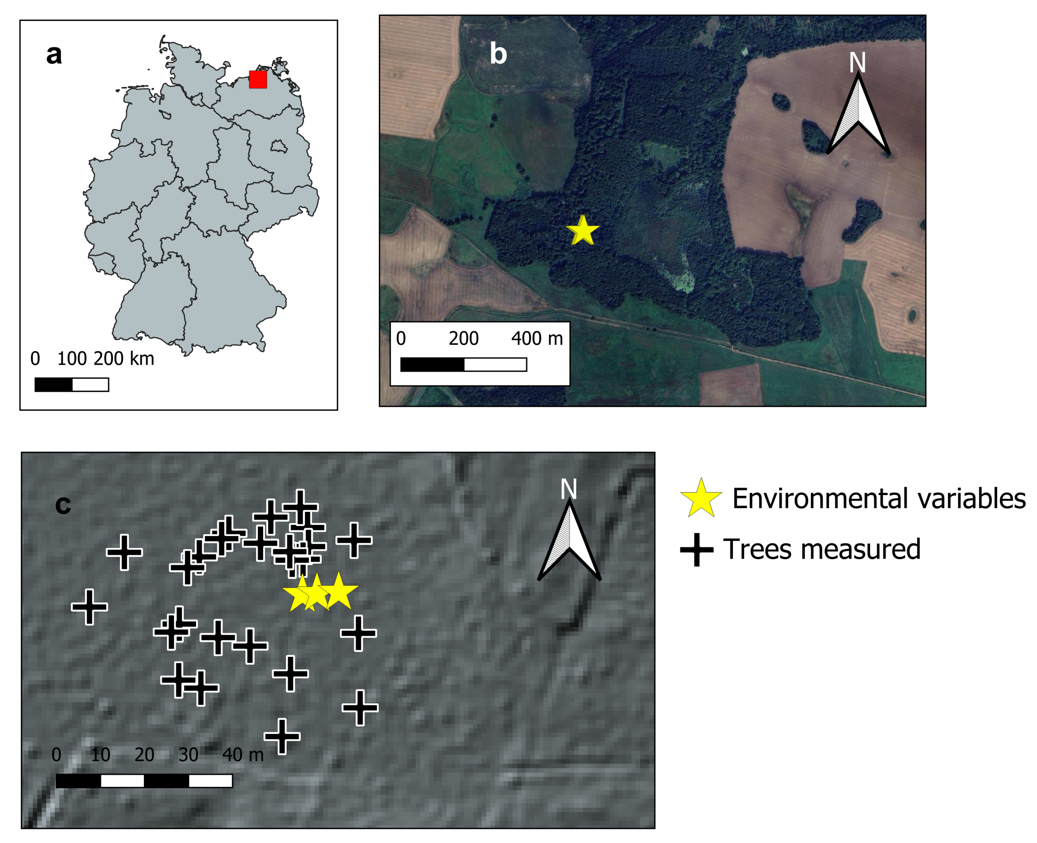
Figure 3.
(a) Average soil temperature at 5 and 15 cm depth measured at three spots within the stand and water level measured at one spot, (b) Sap flux density (shading represents standard deviation)
Figure 3.
(a) Average soil temperature at 5 and 15 cm depth measured at three spots within the stand and water level measured at one spot, (b) Sap flux density (shading represents standard deviation)
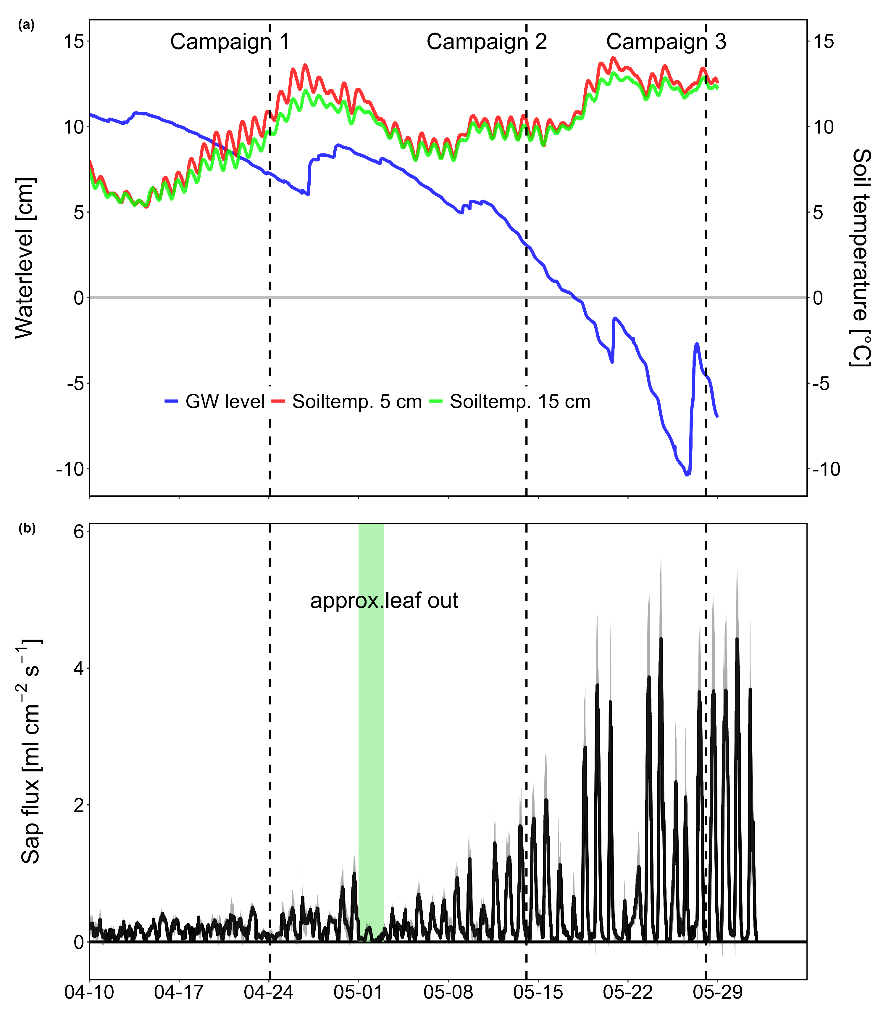
Figure 4.
Figure 4: Average stem CH4 fluxes ordered by their magnitude.
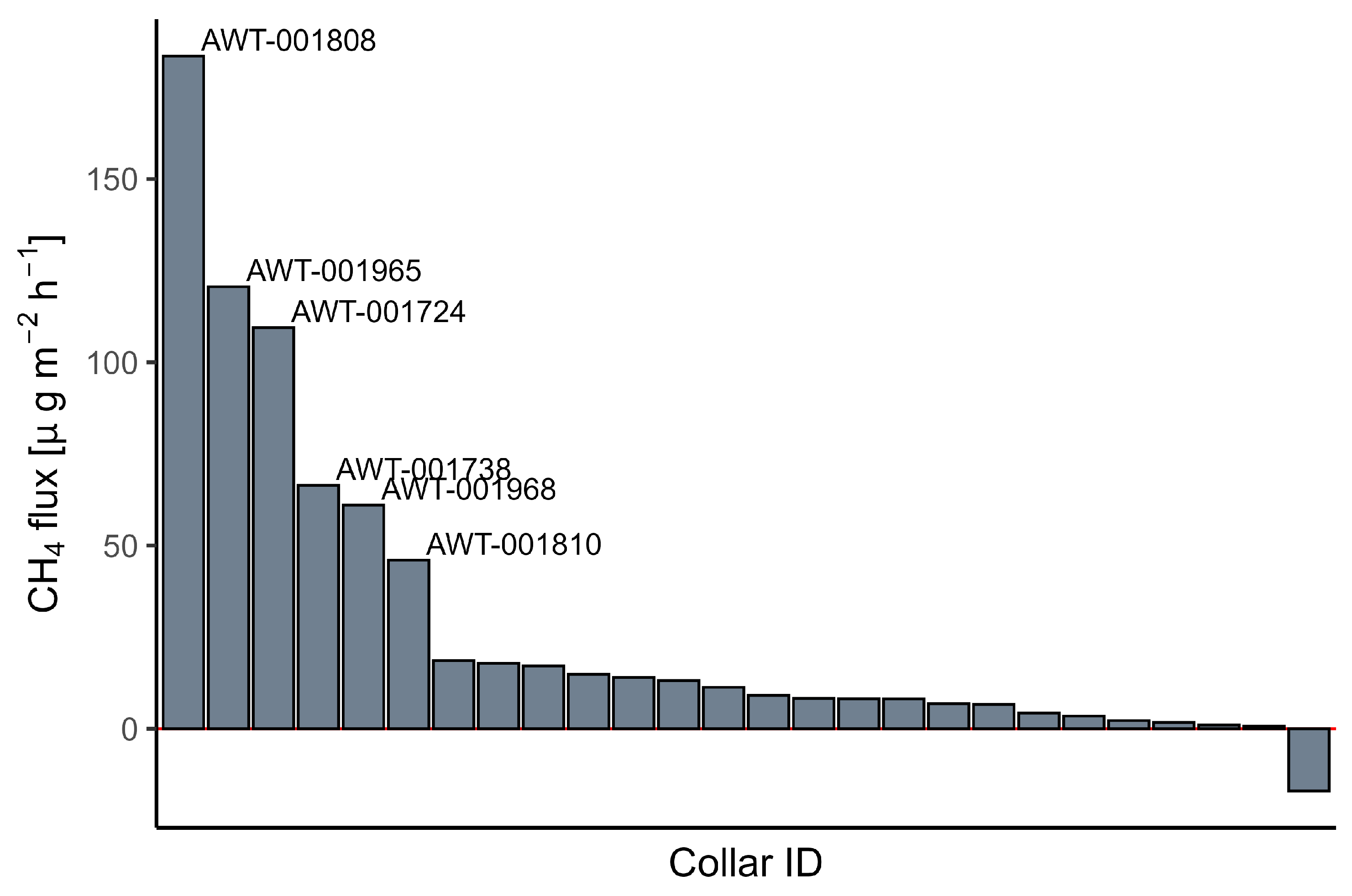
Figure 5.
Relationships between (a) stem CH4 flux orthometric height, (b) CH4 flux and CO2 flux and (c) between CH4 flux and height above stem base (HASB)
Figure 5.
Relationships between (a) stem CH4 flux orthometric height, (b) CH4 flux and CO2 flux and (c) between CH4 flux and height above stem base (HASB)
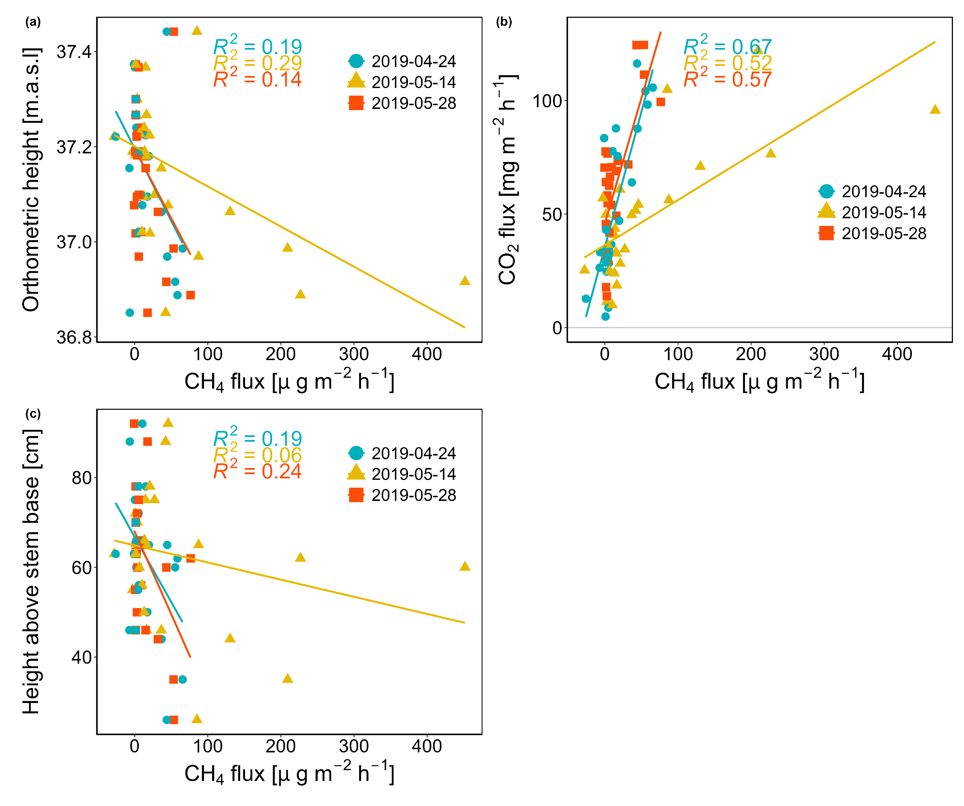
Figure 6.
Visual overview of the spatial variability of stem CH4 fluxes (colours) and orthometric height (size of circles).
Figure 6.
Visual overview of the spatial variability of stem CH4 fluxes (colours) and orthometric height (size of circles).
Disclaimer/Publisher’s Note: The statements, opinions and data contained in all publications are solely those of the individual author(s) and contributor(s) and not of MDPI and/or the editor(s). MDPI and/or the editor(s) disclaim responsibility for any injury to people or property resulting from any ideas, methods, instructions or products referred to in the content. |
© 2025 by the authors. Licensee MDPI, Basel, Switzerland. This article is an open access article distributed under the terms and conditions of the Creative Commons Attribution (CC BY) license (http://creativecommons.org/licenses/by/4.0/).
Copyright: This open access article is published under a Creative Commons CC BY 4.0 license, which permit the free download, distribution, and reuse, provided that the author and preprint are cited in any reuse.


