Submitted:
24 January 2025
Posted:
24 January 2025
You are already at the latest version
Abstract
Agriculture is a backbone of Ethiopian economy, contributing a vital role to food security and employment in rural communities. Climate change and variability have been adversely influenced, challenging the country’s efforts to ensure food security. As a result, this study investigated the association between climate variability and tuber crop yields in southern Ethiopia. Modified Mann-Kendal trend test and coefficient of variation were implemented to examine trend and variability while Seaborne bivariate kernel density was used to assess how climate variability has been related with tuber crop yields. The study has also evaluated the predictive potential of multivariate regression by means of coefficient of determination and root mean square error metrics. The rainfall characteristics showed increasing trend during spring, autumn and annually at a rate of 0.32 mm, 1.67 mm and 0.25 mm, whereas significantly decreasing in summer rainy season at a rate of 0.455 mm/year. Spring and autumn rainfall revealed moderate to high variability, posing risks to rain-fed farming. Days and night time showed increasing trend at a rate of 0.053 oC and 0.16 oC 1981-2021 period. A reasonable tuber crop yield was harvested with cumulative rainfall ranging from 450.0 to 650.0 mm during the growing season, day and night time temperature was between 23.0-26.0 oC and 11.5-14.0 oC. When day time temperature above 26.0 oC and night time temperature below 11.5 oC, sweet potato and taro yields decrease, and harvesting is utterly unexpected. The RF regression model proved to be the best model performing algorithm allowing for optimal yield prediction, assisting farmers and decision makers in better planning crop production and management. The high variability of spring rainfall and the decreasing trend of summer rainfall, combined with an increasing of temperatures, could reduce agricultural productivity, leading to food insecurity. Therefore, the yield of tuber crops can be improved by supplementing the rain-fed farming system with irrigation and applying modern farming techniques and operations by farmers. Moreover, the finding suggests that the need to carefully select plant varieties tolerant to high ambient temperature conditions, which will be more prevalent in the context of climate change. There is a need to intensify adaptation measures to minimize the negative consequences of climate variability to improve the adaptive capacity of sweet potato and taro farmers.
Keywords:
Agriculture
; rainfall
; Random Forest regression
; sweet potato yields
; taro yields
; temperature
; variability
; Wolaita
1. Introduction
The Intergovernmental Panel on Climate Change (IPCC) Assessment Report Six (AR6) indicated that human practices through releasing radiative active greenhouse gases have evidently triggered global warming. Historical records show an increase in global surface temperature by 1.1 oC since 1950 [1]. According to the same source, several changes in extremes are a direct result of increased radiative forcing of greenhouse gasses in the atmosphere both globally and, to some extent county-wide. The global warming is associated with changes in large-scale hydrological cyclic events, such as an increase in atmospheric water vapour, shifting rainfall patterns, changes in rainfall intensity and seasonal to annual variations [2]. A literature review indicated that the increasing of temperature increases the intensity of evaporation and rate of falling of condensed water vapor, cause changes in the weather patterns that characterize climate of specific area [3]. Moreover, the water holding capacity of air parcel also increases with every 1 oC rise in ambient air temperature that would have adverse impact on hydrological process [4]. As a result, the water gripping capability of the air parcel increases, leading to changes in vertical stability and meridional temperature gradients [5]. Thus, the changing climate influences on climate dynamics of onset, secession, spatio-temporal distribution and amounts [6] [7]. Potential future changes in rainfall and temperature are likely to increase, especially in East African countries, and are more likely to warm by the end of the century according to different scenarios compared to the reference period [8]. In Ethiopia, rapidly increasing temperature has projected to be warmer at the end of a century [9].
According to United Nation Development Program (UNDP), the mean yearly temperature has increased via 1.3 oC between 1960 and 2006, with an average rate of 0.28 oC per decade [10]. At a station level, mean annual temperature has increased at a rate of 0.81 oC to 1.68 oC, indicating greater than the rate of change found at national level [11]. Other researchers emphasized that annual minimum and maximum temperature significantly increased at stations level in the period of 1993-2022 [12]. The strong inter-annual and inter-decadal variability in Ethiopia’s rainfall and its linkages with atmospheric drivers makes it difficult to detect long-term trends [13]. However, station-level studies have shown an increasing trend at some weather stations and a decreasing trend at other stations. For example, rainfall from June to September has shown a decreasing trend at some weather stations and an increasing trend at other stations with high interannual variability. [14]. Other scholars also noted that the annual, spring and summer rainfall significantly increased while autumn and winter rainfall revealed decreasing trend with varying magnitude [12].
The consequence of climate change is more pronounced in developing nations due to highly reliance on rain-fed agriculture, and have low adaptive capacity of a societies [15]. The situation is more severe in Sub-Saharan countries like Ethiopia, due to its highly reliance on rain-fed agriculture practiced by smallholder farming systems [16]. Smallholder farming is the primary agricultural activity, providing 84% of the country’s livelihoods [17]. Studies indicated that rainfall based crop cultivation is adversely affected by climate change and its variability causing food insecurity [18]. Ethiopia has a wide range of agro-ecological zones ranging from higher altitude greater than 4550 meter above mean sea level to lower altitude to 160 meter below mean sea level [19]. The country’s location close to the equator provides bimodal rainfall types that periodically circulate [20]. The first period occurs throughout spring season spanning from February to May, while the second occurs during the summer season spanning from June to September bringing longer rainy season [21]. Therefore, rain-fed agriculture dominates many farming activities in the country, and is well kwon for high crop diversity [22].
According to the Central Statistical Authority (CSA) of Ethiopia, the numerous types of crops farmed by smallholders across the country include cereals, tubers, cash crops, and oil crops. Among roots and tuber crops, sweet potato and taro are important crop served as stample or subsistence food by millions of people accros a country. They provide a substancial part of the country’s food supply and are also an important source of food security for rapidly growing population [23]. They are grown throughout the world, however, particularly grown tropical areas, with an altitude of 1700 to 2700 meter above mean sea level [24]. Sweet potato yield is Early maturing tuber crop, can be harvested three to four months after planting, providing food security across many Sub-Saharan African countries. Temperature and amount of sunny days have a significant impact on sweet potato yields. If temperatures are low, the growing season must be extended to six to seven months, and if there are many overcast days, production would be reduced with low root quality [24]. On the other hand, taro can grow in areas above mean sea level of 1800 meter [25]. These crops are more prized, because they are grown under different growing seasons, warm and humid climate of diversified agro-ecology [26]. Moreover, they are an adaptable crop that produces large amounts of food per unit area and per unit time, giving it an advantage over other staple foods [27].
Despite the vital contribution to food security, yield of tuber crops remained below the global average leading to poor yield at farm level. Studies indicated that it is significantly affected by both biotic and abiotic including lack of adaptable cultivars, low availability of improved seed varieties, inadequate of irrigation, weak attitude of people toward tuber crops and inefficient means of technology transfer [28]. On the other hand, tuber crops are highly threaten by extreme climatic conditions derived by ongoing global warming [29]. Other authors explained that tuber crop production is significantly constrained by climatic stress [30]. As a result, the average yield produced by peasants are far lower than the global average in Ethiopia [31]. This is since extreme weather conditions, such as climate change and fluctuation, are detrimental to most crops performance and have an impact on the predicted quantity of agricultural output [32]. While there is no way to totally eliminate such devastating hazard, it would be much better if decision makers and farmers have sufficient information about the future, so that they can plan accordingly [33]. Examining the spatial and temporal dynamics of climate variables and their relationships with crop production and productivity is essential to recommend appropriate adaptation measures at farm-level and improve productivity [34]. Moreover, sharing early information about predicted crop production could help to reduce the likelihood of food insecurity.
In this regard, this study was aimed to investigate spatio-temporal climatic trends and variability, to analysis the relationship between climatic variables with tuber crop yields such as sweet potato and taro harvests, and to evaluate the predictive potential of three machine learning models. Three machine learning models are used to identify the best model in the future for crop yield prediction, named as a Regression, XGBRegression and Random Forest Regression. Modified Mann-Kendal (MMK) trend test and coefficient of variation were implemented to analysis the trend and variability. Seaborne bivariate kernel density estimate (KDE) were used to ascertain the relationship between tuber crop yields (sweet potato and taro) and climatic variables (rainfall, maximum and minimum temperature).
2. Materials and Methodology
2.1. Description of the Study Area
The Wolaita zone is located in the southern Ethiopia, within 6.40 to 7.10 N latitude and 37.40 to 38.20 E longitudes, respectively (Figure 1). It covers the total land mass of 4,511 Km2. Study by scholars described wolaita zone into three agro-ecological categories named as mid-latitude (covers about 56%) of land mass, low latitude (covers about 35%) and high latitude (covers nearly 90%), respectively [35].
There are only 10 weather stations site in the study area. As a result, a virtual network of stations with long and comprehensive time series of meteorological data covering the study area. The virtual dataset was extracted from National Aeronautical and Space Authority (NASA), and here was employed to fill the gap in the gauge dataset and improve stations distributions.
Wolaita farmers practice small-holder home gardening with mixed crops supported with livestock. The Wolaita zone is the highest tuber crop growing regions in Ethiopia [30]. It is one of the most densely populated zones in a country, with a population of over 1.8 million, and with 290 inhabitants per km2 [36]. As a result, the land-holding size is relatively small and most inhabitants are subsistence peasants [37]. According to the Central Statistical Authority (CSA), a range of crops are grown by peasants in Wolaita zone, including cereal, tuber crops and oil crops [23]. Among tuber crops, all peasants grow sweet potatoes and Taros as their primary food crop, both for their own use and the market [38]. These crops play an important role in filling the gap in household food requirement particularly during the dry season [38].
2.1. Research Design and Data Sources
Regarding dataset, a daily time series of rainfall, maximum and minimum temperature were acquired from Ethiopian Meteorology Institute (EMI), on behalf of temporal coverage of 1981-2021 period. Since the gauge dataset has a missing, and the quantity of missing data gap in the range of 1.9% to 96.1% for rainfall, 5.3% to 96.9% for maximum temperature and 6.3% to 97.1% for minimum temperature, respectively (Appendix A 1). Since the gauge dataset has missing, we used global energy resource prediction made by the National Aeronautics and Space Administration (NASA) reanalysis product to fill missing in observation. This dataset is an appropriate substitute used by many scholars over African countries, and formed by NASA's Global Modeling and Assimilation Office (GMAO) [39] [40]. The dataset is downloaded via https://power.larc.nasa.gov/data-access-viewer/ and obtained by entering the target location's latitude and longitude and transferred to a netCDF or CSV format. The quality of NASA dataset has been check by Root Mean Square Error and Pearson Correlation coefficient with observed time series (Appendix A 2).
Regarding agricultural dataset, tuber crop yield such as Sweet potato and Taro yields reported in quantal per hectare (qt ha-1) cultivated by small-holder’s peasant obtained from CSA of Ethiopia for 2002-2016 period. According to [41], tuber crop yields are relatively consistent. This tuber crop is widely grown in the study area by small-scale landowners and play an important role in filling the food security of household particularly during the dry season [42].
2.2. Data Quality
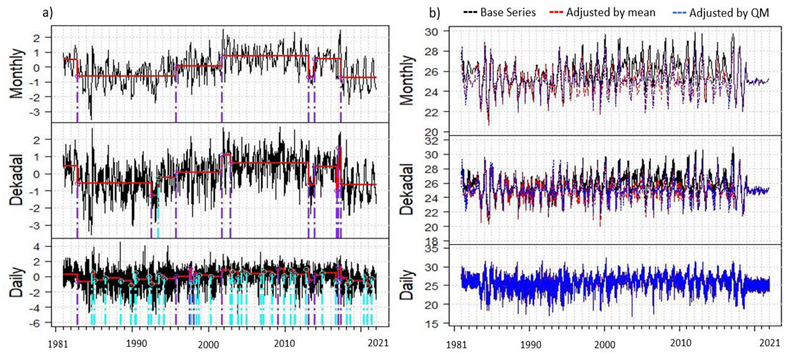
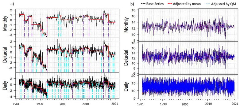
One key problem with using climate time series is existence of data gaps. Thus, these data gaps had to be properly filled and quality-controlled to provide reliable, continuous and homogenous reference time series in which differences are only caused by weather and climatic variability [43]. However, few climate time series are free from non-natural irregularities. This inhomogeneity is related to the process of collecting, digitizing, processing, transferring, storing and transmitting climate data series. As a result, Standard Normal Homogeneity Test (SNHT) created by Alexanderson (1986), is used to identify inhomogeneity in time series [44]. The detected heterogeneity is adjusted using the quantile mapping (QM) and mean value. Among heterogeneity correction methods, the most widely used correction methods are those based on QM approach [45]. Sample result of inhomogeneity adjusted time series for rainfall, maximum and minimum temperature are indicated in Appendix B 1, Appendix B 2, and Appendix B 3, respectively.
2.3. Methods of Data Analysis
2.3.1. Trend Detection
The non-parametric Mann-Kendall (MK) statistical test has been popularly used to assess the existence of trend [46]. The test requires sample data to be serially independent, and when serially correlated in time series, it affect the ability of the test to correctly asses the presence of trend. To eliminate the effect of serial correlation in original MK test, the Modified Mann-Kendal (MMK) test is used to perceive statistically significant decreasing/increasing patterns in extended temporal dataset. This approach is widely used by other scholars for serially correlated data by means of variance correction approach [47]. According to [47], MMK is proposed to remove the influence of serial correlation on original MK trend test. MMK trend test is predicated on two theories, one of which is null (), other is the alternative () hypotheses. The indicates that there is no trend, whereas clarifies whether there is a notable rising or
falling tendency in temporal time series dataset. Depending on a five percent
threshold significant, if the p-value is less than 0.05, the alternative
hypotheses is acknowledged, indicating the existence of an inclination in a
dataset, additionally, if the p-value is higher than 0.05, null hypotheses
would be recognized as indicating that there is no trend in a dataset. The
computational steps for trend are provided by the Eq.1.
Where and were monthly, seasonal and year values, j and i years that j>i, and there are n quantity of data points. Assuming θ, the value of sign (θ) computed as follows using Eq.2:
The trend direction is denoted by the sign of . The increasing trend can be mentioned as significant, if the positive value of Z is greater than 1.96 and the trend is inferred to be decreasing if the negative value of Z is less than -1.96, respectively. Furthermore, a rising trend in the dataset is shown by a positive value of S, whereas a falling trend is indicated by a negative value [48], and calculated according to Eq.3.
The preceding section demonstrated original MK trend test that did not identify serial correlation in time series dataset. The existence of serial correlation alters the variance of the original MK statistics. Therefore, by modifying the variance using effective sample size limit the effect of serial correlation. To eliminate the influence of serial correlation on the original MK, the following equations are implemented, Eq 4:
Where is the actual sample size (ASS), is the effective sample size (ESS) and is termed as the correction factor, respectively. The ESS is given according to [49] as Eq 5:
Where is the lag-k serial correlation coefficient which can be represented by the sample lag-k serial correlation coefficient as given by [50], and calculated as Eq 6:
As explained by [51], the formula for computing at lag-1 autoregressive process and serial correlation coefficient () is computed as Eq 7:
The magnitude of a trend is evaluated by a simple non-parametric procedure using Sen's inclination estimation developed by [52], estimated by means of Eq. 8 as follows:
Where i = 1 to n-1, j = 2 to , and are data values at time j and i where (j > i), respectively. If there are n values of in the time series, Sen’s slope estimator will be N=n(n-2)/2. The Sen’s slope estimator is the mean slope of N values, then, the Sen’s slope is estimated using Eq.9:
The positive value of indicates an increasing trend, while the negative value of shows declining trend, where the units of Sen’s slope () is the slope per year in temporal dataset.
Rainfall and temperature variability was analyzed using coefficient of variation (CV) defined as the ratio of standard (SD) deviation to the mean and quantified the inter-annual variability. According to some author, the level of variability is classified as low variability (CV ≤ 20%), moderate variability (20% ≤CV ≤30%) and high variability (CV > 30%) [53].
2.3.2. Climate and Crop Yield Association
The relationship between root crop yield and climate variables were investigated using Pearson correlation coefficient. The correlation coefficient r ranges from minus 1 to plus1, entire independency of the variables are represented by 0, while complete dependency among 2 variables are written as -1 or +1, respectively. When the value of r is 0.1, it is taken as small, 0.3 is taken as medium and 0.5 is taken as large [54]. The Pearson correlation coefficient r is computed using Eq.10 as:
Whereby ·x is the average of the explanatory variables, r is the correlation coefficient, and x is the independent variable, y is dependent variables and is average of reliant variable, respectively. The correlation coefficient strength show from +0.1 to +0.29, +0.3 to +0.49 and +0.5 to +1 interoperated as weak/small, moderate/medium and strong/large positive correlation while from -0.1 to -0.29, -0.3 to -0.49 and -0.5 to -1 is considered as weak/small, moderate/medium and strong/large negative correlation as explained by [55].
2.3.3. Model Performance
In this study, before training the model, the dataset was divided into two parts: one for training and the other for testing. 80% of the data was used to train the model and the remaining 20% to test the model. Rationally, the relationship between climate and crop growth and development is more complex, and with 80% training, the model could learn more complex patterns and relationships. Empirical studies show that the best results are obtained by using 20-30% of the data for testing and the remaining 70-80% for training [56]. The potential predictability of the models was evaluated using coefficient of determination (R-2) and root mean square error (RMSE), respectively. R-2 describes the degree of variation in the explanatory variable explains, and its values vary from 0 to 1 and are usually indicated as percentages between 0 and 100. Considering the dataset has n values ……, (known as ), each associated with a fitted or predicted values ……., (known as ). Then, the residual values are defined as Eq 11:
Where is mean of observed dataset
The variability of the dataset can be measured with two sums of squares formula. The total sums of squares, which is given as Eq 13:
The sum of squares of residuals is given as follow:
The computation of the coefficient of determination is given as follow, Eq 15:
The RMSE has been used as a standard statistical metric to measure model performance in meteorology, air quality, and climate research study [57]. The RMSE refers to the deviation between the observed dataset and the predicted value.
For example, a sample of n observations and y (, i=1,2……., n) where is the observation and is represents predictions, is mean of observation, the RMSE is computed as follow, Eq 16:
3. Results
3.1. Rainfall
Temporal statistical characteristics of monthly rainfall spanning from 1981 to 2021 period were shown in Figure 2. For graphical presentation, three stations were randomly selected, and named as Bombe, Areka and Bilate, respectively. The monthly rainfall pattern indicated that the lowest rainfall was in the month of December with magnitude of 20.0 mm at Bilate station, 20.4 at Areka station and 22.3 mm at Bombe station, respectively. The highest monthly rainfall various from 133.7 mm at Bilate station in the month of April, 179.0 mm at Areka station in the month of May and 205.9 mm at Bombe station in the month of August, respectively. Spatially averaged monthly rainfall various from 21.3 mm in the month of December to 179.9 mm in the month of May (Figure 2a). However, the rainfall maxima various from station to station. For example, the peak rainfall is in the month of April and May at Bilate and July and August at Areka and Bombe stations, respectively. Moreover, there are two peak rainfall period, April-May and September-October at Bilate station, April-May and July-August at Areka and Bombe stations (Figure 2). The study area receives bimodal rainfall pattern that occurred from February to May and June to September (Figure 2). The peak rainy season occurs in the month of July to September (summer season) and March to May (spring season) locally known as Belg and Kiremt, respectively (Figure 2).
The monthly rainfall pattern indicated the highest rainfall was contributed to annual rainfall in the month of May and July with 13.34% and 13.02%, respectively. While the lowest rainfall was contributed in the month of December (1.55%) and January (2.09%), respectively (Table 1). According to CV, rainfall was highly variable in the month of October, November, December, January, February, March April and moderately variable in the month of May, June, July and low variable in the month of August and September, respectively (Table 1). The MMK trend test indicated increasing trend in the month of February, March, April, May, June, October, November and December respectively. On the other hand, decreasing trend revealed in the month of January, July, August and September, with magnitude of 0.02, 0.169, 0.136 mm per month (Table 1). The dry season months have higher CV, indicating the instability of rainfall occurrence above/below the long term mean value over a particular period.
Table 2 Show statistics of spring, Summer, Autumn and annual rainfall characteristics and percent of contribution to annual rainfall. Over the study area, the mean annual rainfall varies from 1134.6 mm at Humbo station to 1526.3 mm at Bele station, respectively. During spring, summer and annually, the highest rainfall was recorded at Bele station, with magnitude of 555.1 mm, 704.3 and 1526.3 mm, respectively. On the other hand, annually and spring season, the lowest rainfall was measured at Humbotebela station, with magnitude of 1134.6 mm and 209.0 mm, respectively. During summer season, the lowest rainfall was recorded at Bilate station with magnitude of 495.4 mm (Table 2). Spatially averaged annual rainfall was 1324.8 mm, 490.72 mm in spring and 602.92 mm in summer season, respectively (Table 2). The summer season contributes the highest rainfall at all stations with 42.9% of contribution at Bilatetena station to 48.1% of contribution at Bele station, respectively. Spring season was the second higher contributors of annual rainfall in the range of 35.2% at Wolaita station to 37.9% at Bilatetena station, respectively (Table 2).
The annual rainfall trend analysis indicated decreasing trend at 70% of weather stations while increasing trend at 30% of weather stations, respectively. But the decreasing or increasing of annual rainfall trend was not significant at 0.05 significant level. The spring rainfall trend analysis indicated increasing trend at 90% of meteorological stations while decreasing trend at 10% of meteorological stations. Moreover, three stations (Areka, Bombe and Wolaita) indicated significantly increasing trend at a rate of 2.16 mm/year, 0.048 mm/year and 2.24 mm/year, respectively. The summer rainfall indicated decreasing trend at 60% of weather stations, but not significant at 0.05 significant level (Table 2).
The annual and seasonal rainfall variability analysis was presented in Figure 3. According to CV, the rainfall various from one station to other stations, and from one season to other seasons. For example, the coefficient of variation was in the range 10.9% to 15.9% in summer season, 13.2% to 33.8% in spring season and 63.4% to 77.8% in autumn season, respectively (Figure 3a-d).
3.2. Temperature
Figure 4 Shows monthly maximum, mean (average of maximum and minimum) and minimum temperature characteristics at Areka, Bilate, Bombe and spatially averaged. Accordingly, July is the coldest month with monthly minimum temperature value of 11.2 oC, 12.0 oC and 13.4 oC at Areka, Bilate and Bombe stations, respectively (Figure 4c). While February is the warmest month with monthly maximum temperature value of 28.4 oC, 32.0 oC and 27.7 oC at Areka, Bilate and Bombe stations respectively (Figure 4a). Spatially averaged monthly minimum, mean and maximum temperature in the range of 12.1 oC to 13.5 oC, 18.2 oC to 20.6 oC and 24.3 oC to 27.8 oC (Figure 4a-c). The temperature characteristics at station level indicated that monthly maximum temperature value was 24.2 oC to 28.4 oC at Areka station, 28.2 oC to 32.2 oC at Bilate station, 22.7 oC to 27.7 oC at Bombe station, respectively. The mean temperature value at station level was 17.7 oC to 20.5 oC at Areka station, 21.3 oC to 23.6 oC at Bilate station, 17.4 oC to 20.4 oC at Bombe station. Whereas monthly minimum temperature was in the range of 11.2 oC to 13.4 oC at Areka station, 13.4 oC to 15.7 oC at Bilate station, 12.0 oC to 14.2 oC at Bombe station respectively (Figure 4a-c).
The annual mean, maximum and minimum temperature observed at each meteorological stations were analyzed at Table 3. Accordingly, the annual maximum temperature was 24.4 oC at Bombe station to 33.3 oC at Bele station, respectively. The annual minimum temperature was 12.0 oC at Bombe station to 17.1 oC at Bele stations. Annual mean temperature was 18.5 oC at Bombe station to 23.7 oC at Bele station, respectively. Spatially averaged annual minimum, mean and maximum temperature was 12.8 oC, 19.4 oC and 26.1 oC, respectively (Table 3). Annual maximum temperature analysis indicated increasing trend nearly at all meteorological station. For example, the annual maximum temperature indicated significantly increased at Bedessa, Bele, Bilatetena, Gessuba and Wolaitasod stations, with magnitude of 0.04 oC, 1.69 oC, 0.033 oC, 0.017 oC and 0.029 oC, respectively. On the other hand, annual minimum temperature has shown positive trend toward increasing nearly all weather stations (Table 3). Moreover, the spatially averaged annual maximum temperature indicated significantly increased, the Wolaita zone warmed by 0.053 oC (Table 3).
3.3. Yield trend and variability
Figure 5: Below indicates sweet potato and taro yield anomalous and trend for 2002 to 2016 period. The result of trend analysis indicated that both sweet potato and taro yield was increased during the studied period. However, low yield amount harvested in the year of 2005, 2006, 2007, 2008, 2009, 2010 and 2016 for both crop yields, respectively. The coefficient of determination indicated 50.33% and 46.67% of yield variability explained during the study period (Figure 5a-b).
Table 4 Below indicates descriptive statistics of sweet potato and taro yield. The standard deviation, minimum, mean, maximum and coefficient of variation for Taro yield were 103.5 qt/ha, 85.8 qt/ha, 188.2 qt/ha, 378.7 qt/ha and 55.0% (Table 4). Similarly, standard deviation, minimum, mean and maximum for sweet potato yield were 89.9 qt/ha, 80.0 qt/ha, 166.4 qt/ha, 327.0 qt/ha (Table 4). According to coefficient of variation, taro and sweet potato crop production was highly variable with cv of 55.0% and 54.0%, respectively. However, the MK trend test revealed that taro and sweet potato yield was increased at a rate of 6.069 qt/ha and 5.36 qt/ha of land (Table 4).
3.4. Relationship Between Climatic Variables and Tuber Crop Yields
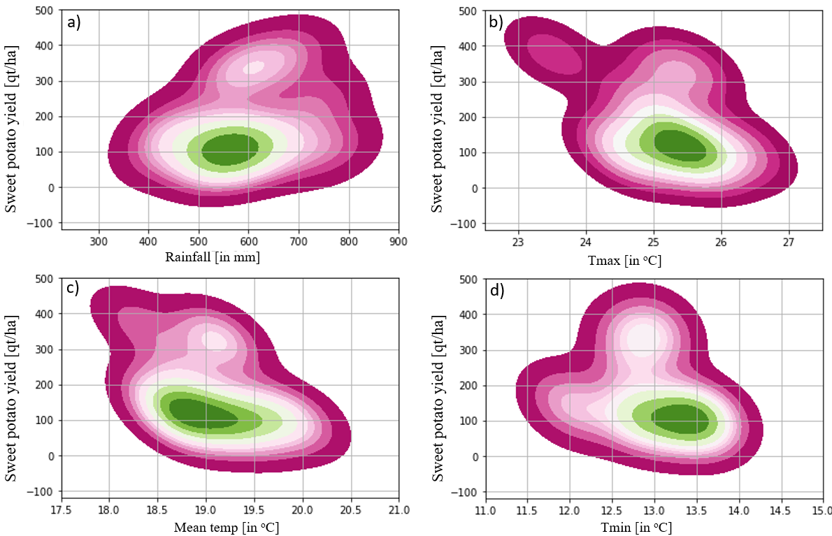
The bivariate kernel density estimate (KDE) was implemented to ascertain the association between climatic variables and tuber crop yields, respectively. Figure 6 and Figure 7 indicate KDE between growing period climatic variables and tuber crop yields. According to KDE, sweet potato was positively related with growing period rainfall while negatively related with maximum, minimum and mean temperature. As growing period rainfall increased from 350.0 mm to 800.0, sweet potato was increased from150 qt/ha to 400.0 qt/ha of land. On the other hand, the highest yield harvested when growing period rainfall was between 600.00 mm to750.0 mm, and the high density distribution was observed when the rainfall amount of 700.0 mm that resulted in the production of nearly 475.0 qt/ha of land (Figure 6a). Likewise, the investigation of crop temperature requirements has been evaluated using Seaborne kernel density estimate. According to Figure 6, to achieve a good harvest of sweet potato, the daily maximum, mean and minimum temperature required should be between 23.0 oC to 26.5 oC, 18.0 oC to 20.5 oC and 11.5 oC to 14.0 oC during the growth and development period (Figure 6b-d).
As indicated bivariate kernel density estimate, taro yield was positively related with rainfall while negatively related with maximum, mean and minimum temperature. According to Figure 7, as rainfall increase, taro yield increased but maximum, mean and minimum temperature increase taro yield decreased (Figure 7a-d). The high-density distribution was observed around 750.0 mm rainfall and resulted good harvesting of taro yield nearly 400.0 qt/ha of land (Figure 7a). On the other hand, the temperature pattern indicated that the high density distribution of taro yield was obtained between 24.5 oC to 26.0 oC of Tmax, 18.0 oC to 19.5 oC of mean temperature and 12.5 oC to 13.5 oC of minimum temperature and harvested 300.0 qt/ha of land (Figure 7b-d).
3.5. Yield Prediction and Model Performance Evaluation
Predicting crop yield by means of machine learning is an important topic since it provides information about productivity trends for decision making. In this study, the sweet potato and taro yield dataset were trained with three models to determine the best crop yield predictor to propose for further work. Although there are other climate-related predictors of agricultural production, rainfall and temperature have been utilized due to the lack of additional variables such as humidity, soil moisture, and solar radiation. As indicated in Table 5, the models performance were compared by means of RMSE and R-squared values. The trained and tested models showed that the accuracy for sweet potato yield forecasting by means of RMSE was 142.76, 148.38 and 0.2415 qt/ha of land for GBR, XGBR, RF and MLR, respectively. In contrast, the RMSE for predicting taro output was 172.28, 205.32, 127.24 and 0.3676 qt/ha of land for GBR, XGBR, RF and MLR, respectively (Table 5). GBR, XGBR, RF and MLR had predictive values of 0.7699, 0.7499, 0.7970, and 0.2415 explained sweet potato yield, and 0.7759, 0.6899, 0.7793, and 0.3676 for taro yield based on R-squared metrics (Table 5).
4. Discussion
The apparent temporal fluctuation in rainfall and temperature has far-reaching implications for smallholder farming system. Adequate and timely rainfall during agricultural/cropping seasons is crucial to farming activities. However, unpredictable rainfall triggered by fluctuation, erratic nature and inconsistency during the growing season, rain-fed smallholder farmers suffer from food insecurity [19]. Along with insufficient soil moisture to sustain crop farming as a result of evaporation and transpiration due to increased temperature, reduces agricultural productivity and production [58]. During the study period, rising temperatures may have had a substantial impact on smallholder farmer’s farming practices. It would exacerbate the occurrence of drought, limiting soil moisture availability and crop-land productivity, leading to crop failures [59]. According to the evidence shown above, agricultural production is reduced by rainfall and temperature variability, which has an impact on agricultural sector, which significant contributors to food security and employments across a country. Therefore, climate variability has a potential implication on agriculture because it is very susceptible to climate change and variability [60].
The rainfall analysis showed bi-modal characteristic with spatial-temporal variation across meteorological stations (Figure 3). The coefficient of variation indicated that June-September rainfall experienced low variability. While spring and autumn rainfall experienced moderate and high variability, contributing 35.7% and 16.5% to the total annual rainfall, respectively, with associated risks to rain-fed crop cultivation (Table 2). Spatially averaged annual, spring and autumn rainfall increased at a rate of 0.275 mm/year, 0.32 mm/year and 1.67 mm/year. Whereas June-September rainfall has significantly decreased at a rate of 0.455 mm/year during crop growing period. Maximum and minimum temperature indicated significant increasing trend at a rate of 0.053 oC/year and 0.016 oC/year (Table 3). The results of this study are consistence with those of earlier researchers. For example, [12] has shown that summer rainfall tends to decline while autumn and winter rainfall tend to increase. Previous studies in southern Ethiopia found inter-annual fluctuations in temperature and rainfall [53]. A comparable study in the Wolaita zone revealed a considerable increase in temperature and a decrease in rainfall [61]. Other researchers also discovered that rainfall analysis showed significant station-to-station variability (Habte et al., 2023). The inter-seasonal and yearly rainfall variations at meteorological stations exhibited a shifting pattern that drive up and down, with the changes affecting crop output and productivity in diverse way [62].
The environmental response of certain crops relies on the severity of particular weather events, the cultivated species, and the crop’s phonological conditions [63]. Crop water requirements vary from crop to crop, growing season, and specific region [64]. According to the finding of this study, a reasonable tuber crop yield was harvested with cumulative rainfall ranging from 450.0 to 650.0 mm during the growing season, with harvested yield amount of 150-200 qt/ha of land. However, this is only achieved at optimum crop water requirement level. For example, the yield of sweet potato and taro was decreasing below 450.0 mm and above 750.0 mm, respectively (Figure 6 and Figure 7), indicating positive relationship. According to KDE, sweet potato and taro yields were decreased as temperature increased, demonstrating a negative association (Figure 6 and Figure 7). Crop productivity can be affected by above and below optimum temperatures, which result from reduced photosynthesis. Research finding revealed that above or below the optimum temperature has an impact on the performance of the photosynthetic process, resulting in crop failure [33]. According to this finding, the highest density distribution of sweet potato and taro were harvested when the daytime and nighttime temperatures were around 25.0 oC and 13.5 oC, respectively. As daytime and nighttime temperature dip below 23.0 oC and increase above 26.0 oC, and nighttime temperatures decline below 11.5 oC and rise above 14.0 oC, sweet potato and taro yields decrease, and harvesting is utterly unexpected (Figure 6b-c and Figure 7b-c). In general, the harvested sweet potato and taro were maximum at growing season daytime and nighttime temperatures ranging from 24.5-25.5 oC and 12.5-13.5 oC, respectively, with a mean temperature value of 18.0-19.5 oC (Figure 6b-d and Figure 7b-d). The findings correspond with similar work, indicating that as temperature increase, root crop yield decreased, demonstrating a negative association [65]. Another author also suggested that the optimum temperature necessary for the growth and development for root crop was ranged from 19.9 oC to 21.0 oC [66]. The findings of this study revealed that a daytime and nighttime temperature exceed 26.0 oC and go below 14.0 oC, with a mean value exceeding 19.5 oC, have a detrimental impact on root crop growth and development.
The model performance results showed that Random Forest regression is the best model to use in the implementation of an early crop yield prediction, and explaining a high proportion of the variance in sweet potato and taro yield variability. It accounted 79.70% and 77.93% of sweet potato and taro yield variability by combined effect of rainfall and temperature, respectively (Table 5). Other authors have also suggested that RF regression has a high predictive potential and utilized as a machine learning techniques for crop yield prediction [67]. Similar study revealed that crop yield prediction by RF regression produced par results than MLR. For example, RF algorithms attained highest R2 value above 75% [68], and the predictive potential of RF algorithms explained 87% of yield variability [69]. Moreover, [70] noted that the RF algorithms achieved 92.3% of yield predicting.
The full impact of rising temperatures on crop photosynthesis is still being studied, particularly, given the complex interactions of water availability, rising atmospheric carbon dioxide concentration, nutrient availability, plant diseases, and increased frequency and intensity of extreme climate events, all of which feedback to alter crop photosynthesis and productivity [71]. Crop productivity potential could be only determined if a full grasp of crop growth and development is realized. These, in turn, are influenced by climatic, edaphic, hydrological, physiological, use of technology, and managerial aspects. In this study, climate variables are the main drivers to cause year-to-year yield variations. In reality, climate variability is not the only driver to cause major changes to yield variability and trend, there are also other factors, such as radiations, water, nutrition, and pests and diseases [72]. Furthermore, numerous other factors influence crop productivity, including cultivars, crop physiology, and crop management.
5. Conclusion
This study examined temperature and rainfall trend and variability, and explored the relationship between climate variability with rain-fed tuber crop productivity implementing machine learning algorithms. The study has also evaluated the predictive potential of machine learning approaches. The study used climatic variables of rainfall and air temperature as drivers, sweet potato and taro as reliant variables. The analyzed result of rainfall characteristics at station level showed decreasing trend at many stations during summer rainy season, while increasing trend during spring period at many weather stations. Spatially averaged rainfall showed increasing trend during spring, autumn and annually at a rate of 0.32 mm, 1.67 mm and 0.25 mm, while significantly decreasing in summer rainy season at a rate of 0.455 mm/year. Spring and autumn rainfall had moderate to high variability, 20.7% and 38.8%, respectively, posing risks to rain-fed farming, whereas summer rainfall had low variability. Spatially averaged mean, maximum and minimum temperatures showed an increasing trend at a rate of 0.032 oC, 0.053 oC and 0.16 oC 1981-2021 period, respectively. A reasonable tuber crop yield was harvested with cumulative rainfall ranging from 450.0 to 650.0 mm during the growing season, at a day and night time temperature was between 23.0-26.0 oC and 11.5-14.0 oC. When day time temperature above 26.0 oC and night time temperature below 11.5 oC, sweet potato and taro yields decrease, and harvesting is utterly unexpected. Machine learning model, such as RF regression has a good predictive potential, and explained 79.70% and 77.93% of sweet potato and taro yield variability. The study concludes that the high variability of spring rainfall and the decreasing trend of summer rainfall, combined with an increasing of temperatures, could reduce agricultural productivity, leading to food insecurity. While optimal climatic variables might boost crop yield, excessively increased/decreased rates result in declining or even complete failures. The RF regression model proved to be the best model performing algorithm allowing for optimal yield prediction, assisting farmers and decision makers in better planning crop production and management in Ethiopia. Therefore, the yield of tuber crops can be improved by supplementing the rain-fed farming system with irrigation and applying modern farming techniques and operations by farmers. Moreover, the finding suggests that the need to carefully select plant varieties tolerant to high ambient temperature conditions, which will be more prevalent in the context of climate change. There is a need to intensify adaptation measures to minimize the negative consequences of climate variability to improve the adaptive capacity of sweet potato and taro farmers.
Acknowledgments
The author would like to thank the Ethiopian Meteorology Institute for freely providing climate data Ethiopian Meteorological Society and its staff financial supporting for data collecting.
Author Contributions
Tadele Badebo Badacho has solely carried out this research work.
Funding
This research received no fund
Ethics Statement
Informed consent is not applicable
Data Availability
The data used for this research is freely available on reasonable request of the author
Conflict of Interest
The author declares no conflict of interest
Abbreviations
| AR6 | Assessment Report Six |
| CSA | Central Statistical Authority |
| CV | Coefficient of Variation |
| EMI | Ethiopian Meteorology Institute |
| GMAO | Global Modeling and Assimilation Office |
| IPCC | Intergovernmental Panel on Climate Change |
| KDE | kernel density estimate |
| MLR | Multiple Linear Regression |
| MMK | Modified Mann-Kendal |
| NASA | National Aeronautics and Space Administration |
| QM | Quantile Mapping |
| RF | Random Forest Regression |
| RMSE | Root Mean Square Error |
| SD | Standard Deviation |
| SNHT | Standard Normal Homogeneity Test |
| UNDP | United Nation Development Program |
Appendix A
Appendix A.1. Station names, location (latitude and longitude in degree and elevation in meter) and percentage of missing data at each station during the period of 1981 to 2021. The asterisks show stations that are recording only rainfall.
| Stations name | Lat | Lon | elv | Precip (in %) | Tmax (in %) | Tmin (in %) | |
| 1 | Areka | 7.063 | 37.708 | 1758 | 36.2 | ** | ** |
| 2 | Bedessa | 6.869 | 37.936 | 1578 | 4.7 | 20.4 | 23.2 |
| 3 | Bele | 6.918 | 37.526 | 1246 | 27 | ** | ** |
| 4 | Bilate tena | 6.917 | 38.117 | 1499 | 17.5 | ** | ** |
| 5 | Billate | 6.817 | 38.083 | 891 | 5.3 | 15.2 | 17.2 |
| 6 | Boditi school | 6.954 | 37.955 | 1789 | 5.2 | 5.3 | 6.3 |
| 7 | Bombe | 7.138 | 37.584 | 1540 | 96.1 | 96.9 | 97.1 |
| 8 | Gessuba | 6.724 | 37.558 | 1526 | 21.6 | 45.6 | 45.6 |
| 9 | Humbo tebela | 6.702 | 37.759 | 1643 | 19.5 | ** | ** |
| 10 | Wolaitasodo | 6.81 | 37.73 | 1808 | 1.9 | 7.3 | 8.8 |
| The asterisk/** indicates stations that only records rainfall. | |||||||
Appendix B
Appendix B 1, Appendix B 2 and Appendix B 3 Show inhomogeneity detected and adjusted rainfall, maximum and minimum temperature plot at Wolaitasodo station. Wolaitasodo station is here selected due to high percentage of rainfall data availability, only 1.9% missing rainfall, 7.3% missing Tmax and 8.8% missing Tmin, respectively (Appendix A 1). And here Wolaitasodo station desired for graphical representation. The purple dotted line show breakpoint in time series dataset and the red lines show the trend caused by inhomogeneity in time series.
Appendix B 1: Show Homogeinity ajdusted rainfall plot at Wolaitasodo station (a) inhomogenity detected, and (b) inhomogenity ajdusted by mean and ajdusted by QM, respectively.

Appendix B 2: Homogeneity adjusted maximum temperature time series plot (a) inhomogenity detected, and (b) inhomogenity ajdusted by mean and ajdusted by QM, respectively.
Appendix B 3: Homogeneity detected and adjusted minimum temperature time series plot at Wolaita sodo station, (a) inhomogenity detected, and (b) inhomogenity ajdusted QM, respectively.
Appendix A 2 Shows Correlation between NASA reanalysis products and observed dataset at Bilate, Boditi School and Wolaitasodo stations. These stations are selected due to percentage of available data, 1.9% to 5.3% of precipitation missing, 6.3% to 17.2% of minimum temperature missing and 6.3% to 17.2% maximum temperature missing, respectively (Appendix A 1). The correlation coefficient showed (r = 0.23-0.29) for rainfall, (r = 0.75-0.78) for maximum temperature and ( r= 0.28-0.36) for minimum temperature, respectively (Appendix A 2).
Appendix A 2: Correlation result between NASA POWER reanalysis dataset and observation dataset at Bilate, Boditi School and Wolaitasodo stations.
| Reference stations | Tmax | Tmin | precip |
| Bilate | 0.77 | 0.32 | 0.23 |
| Boditi school | 0.75 | 0.36 | 0.26 |
| Wolaita sodo | 0.78 | 0.28 | 0.29 |
References
- IPCC, “SYNTHESIS REPORT OF THE IPCC SIXTH ASSESSMENT REPORT (AR6),” 2021.
- U. Adhikari, A. P. Nejadhashemi, and S. A. Woznicki, “Climate change and eastern Africa : a review of impact on major crops,” 2015. [CrossRef]
- G. K. Gcg and S. Kaur, “Precipitation : Changing Patterns, Crop Effects and Mitigation : A Brief Review,” vol. 3, no. 1, pp. 26–32, 2017.
- K. E. Trenberth, “Changes in precipitation with climate change,” Clim. Res., vol. 47, no. 1–2, pp. 123–138, 2011. [CrossRef]
- S. I. Seneviratne et al., Climate Change 2021: The Physical Science Basis. Contribution of Working Group I to the Sixth Assessment Report of the Intergovernmental Panel on Climate Change. 2021. [CrossRef]
- P. Camberlin et al., “Components of rainy seasons variability in Equatorial East Africa : onset, cessation, rainfall frequency and intensity To cite this version : HAL Id : hal-00334542,” 2009.
- P. O. Omay, O. Christopher, Z. Atheru, and Z. Atheru, Changes and Variability in rainfall onset, cessation and length of rainy season in the IGAD region of Eastern Africa. 2022.
- V. Ongoma, “Projected change in mean rainfall and temperature over East Africa based on Projected changes in mean rainfall and temperature over East Africa based on CMIP5 models,” no. October 2017, 2018. [CrossRef]
- T. Badebo, “Heat Wave Magnitude Projection in the Middle Awash Basin under Coupled Model Intercomparison Project the 6 th phase ( CMIP6 ),” no. June, pp. 1–10, 2023. [CrossRef]
- UNDP, “Climate Change Information Fact Sheet Report country Ethiopia. United Nation Development programme.,” no. September, pp. 8–10, 2015, [Online]. Available: https://www.climatelinks.org/sites/default/files/asset/document/Ethiopia Climate. (accessed on 18.07.2015).
- B. Getachew, “Trend analysis of temperature and rainfall in south Gonder zone, Ethiopia,” vol. 5, no. 2, pp. 1111–1125, 2018. [CrossRef]
- K. Ahmed, Y. Kebede, A. Gelaw, and Y. Mohammed, “Heliyon The trends and spatiotemporal variability of temperature and rainfall in Hulbarag district, Silte Zone, Ethiopia,” Heliyon, vol. 10, no. 11, p. e31646, 2024. [CrossRef]
- A. Alhamshry, A. A. Fenta, H. Yasuda, R. Kimura, and K. Shimizu, “Seasonal rainfall variability in Ethiopia and its long-term link to global sea surface temperatures,” Water, vol. 12, no. 1, p. 55, 2020.
- M. T. Guta, “Rainfall Trends Over Ethiopia,” vol. 30, no. 4, pp. 1–10, 2022. [CrossRef]
- J. H. Kotir, “Climate change and variability in Sub-Saharan Africa : a review of current and future trends and impacts on agriculture and food security,” pp. 587–605, 2011. [CrossRef]
- D. Obsi, D. Korecha, and W. Garedew, “Evidences of climate change presences in the wettest parts of southwest Ethiopia,” Heliyon, vol. 7, no. July, p. e08009, 2021. [CrossRef]
- A. Teshome and A. Lupi, “Determinants of Agricultural Gross Domestic Product in Ethiopia Determinants of Agricultural Gross Domestic Product in Ethiopia,” no. December, 2020. [CrossRef]
- T. B. Badacho, T. D. Geleta, M. D. Lema, S. A. Wondimu, and B. T. Wahima, “Climate Change Impact on Rain-Fed Maize Yield Cultivated with Small-Scale Landowners in Wolaita Zone, Ethiopia,” vol. 9, no. 2, pp. 20–37, 2024.
- H. R. Bedane, K. T. Beketie, E. E. Fantahun, and G. L. Feyisa, “The impact of rainfall variability and crop production on vertisols in the central highlands of Ethiopia,” Environ. Syst. Res., 2022. [CrossRef]
- T. Gissila, E. Black, D. I. F. Grimes, and J. M. Slingo, “Seasonal forecasting of the Ethiopian summer rains,” Int. J. Climatol. A J. R. Meteorol. Soc., vol. 24, no. 11, pp. 1345–1358, 2004.
- E. Viste, D. Korecha, and A. Sorteberg, “Recent drought and precipitation tendencies in Ethiopia,” Theor. Appl. Climatol., vol. 112, no. 3–4, 2013. [CrossRef]
- AfDB, “AfDB-RDGE Country profiles Ethiopia,” AfDB, pp. 1–6, 2021, [Online]. Available: https://www.afdb.org/en/documents/ethiopia-country-profiles-2021.
- CSA, “The Federal Democratic Republic of Ethiopia Central Statistical Agency (CSA) Report on Area, Production and Farm Management Practice of Belg Season Crops for Private Peasant Holdings,” vol. V, p. 25, 2021.
- E. You, E. Wanted, T. O. Know, and A. Sweetpotato, EVERYTHING YOU EVER WANTED TO KNOW ABOUT SWEETPOTATO, no. October. 2018. [CrossRef]
- C. L. Schott, U. Nrcs, and N. Plant, “TARO,” 1967.
- T. Belehu and A. Sciences, “AGRONOMICAL AND PHYSIOLOGICAL FACTORS AFFECTING GROWTH, DEVELOPMENT AND YIELD OF,” 2003.
- L. O. Duque, S. Elsa, K. Pecota, and C. Yencho, “A Win – Win Situation : Performance and Adaptability of Petite Sweetpotato Production in a Temperate Region,” pp. 1–16, 2022.
- A. M. Aldow, “Factors affecting sweet potato production in crop – livestock farming systems in Ethiopia,” 2017.
- U. T. Bekabil, “Review of Challenges and Prospects of Agricultural Production and Productivity in Ethiopia,” Online, 2014. [Online]. Available: www.iiste.org.
- F. Gurmu, S. Hussein, and M. Laing, “Diagnostic assessment of sweetpotato production in Ethiopia : Constraints, post-harvest handling and farmers ’ preferences Diagnostic assessment of sweetpotato production in Ethiopia : Constraints, post-harvest handling and farmers ’ preferences,” no. March, 2015. [CrossRef]
- D. Markos and H. Agricultural, “Agriculture and Food Sciences Research Sweet Potato Agronomy Research in Ethiopia : Summary of Past Findings and Future Research Directions,” no. May, 2019. [CrossRef]
- M. Palmgren and S. Shabala, “Adapting crops for climate change : regaining lost abiotic stress tolerance in crops,” no. December, pp. 1–23, 2024. [CrossRef]
- M. Kuradusenge et al., “Crop Yield Prediction Using Machine Learning Models : Case of Irish Potato and Maize,” 2023.
- A. Asfaw, B. Simane, A. Hassen, and A. Bantider, “Variability and time series trend analysis of rainfall and temperature in northcentral Ethiopia : A case study in Woleka sub-basin,” Weather Clim. Extrem., vol. 19, no. December 2017, pp. 29–41, 2018. [CrossRef]
- T. M. Olango, B. Tesfaye, M. Catellani, and M. E. Pè, “Indigenous knowledge, use and on-farm management of enset (Ensete ventricosum (Welw.) Cheesman) diversity in Wolaita, Southern Ethiopia,” J. Ethnobiol. Ethnomed., vol. 10, no. 1, pp. 1–18, 2014.
- D. H. M. and G. D. Tekola, “Tropical Med Int Health - 2006 - Tekola - Economic costs of endemic non-filarial elephantiasis in Wolaita Zone Ethiopia.pdf.” 2006.
- N. Kebede and H. Mekonnen, “Hydatidosis of slaughtered cattle in Wolaita Sodo Abattoir, southern Ethiopia,” pp. 629–633, 2009. [CrossRef]
- S. Zeverte-Rivza, A. Nipers, and I. Pilvere, “Agricultural Production and Market Modelling Approaches,” Econ. Sci. Rural Dev., no. July, p. 3, 2017. [CrossRef]
- T. Zhang, P. W. Stackhouse Jr, W. Chandler, J. M. Hoell, D. Westberg, and C. H. Whitlock, “A global assessment of solar energy resources: NASA’s Prediction of Worldwide Energy Resources (POWER) project,” in AGU Fall Meeting Abstracts, 2010, pp. U23A-0017.
- R. Gelaro et al., “The modern-era retrospective analysis for research and applications, version 2 (MERRA-2),” J. Clim., vol. 30, no. 14, pp. 5419–5454, 2017.
- L. Cochrane, L. Cochrane, and Y. W. Bekele, “regional and zonal levels,” Data Br., vol. 16, no. 17, December 2017, pp. 1025–1033, 2018. [CrossRef]
- T. M. Beyene, “Exploring Indigenous Knowledge and Production Constraints of Taro ( Colocasia esculenta L. ( SCHOTT )) Cultivars Grown at Dalbo Watershed, Wolaita Zone of South Ethiopia,” no. September, 2015. [CrossRef]
- L. K. Amekudzi, E. I. Yamba, K. Preko, and E. O. Asare, “Variabilities in Rainfall Onset, Cessation and Length of Rainy Season for the Various Agro-Ecological Zones of Ghana,” pp. 416–434, 2015. [CrossRef]
- H. Alexandersson, “Alexandersson, Hans. ‘A homogeneity test applied to precipitation data.’ Journal of climatology 6.6 (1986): 661-675.,” J. Climatol. 1986 - Wiley Online Libr., 1986.
- J. Ringard, F. Seyler, and L. Linguet, “A quantile mapping bias correction method based on hydroclimatic classification of the Guiana shield,” Sensors, vol. 17, no. 6, p. 1413, 2017.
- H. B. Mann, “Non-Parametric Test Against Trend,” Econometrica, vol. 13, no. 3, pp. 245–259, 1945, [Online]. Available: http://www.jstor.org/stable/1907187.
- C. Blain and G. C. Blain, “The modified Mann-Kendall test : on the performance of three variance correction approaches,” 2013.
- R. M. Hirsch, “TECHNIQUES OF TREND ANALYSIS FOR MONTHLY WATER-QUALITY DATA,” vol. 18, no. June, 1981.
- G. V Bayley and J. M. Hammersley, “The" effective" number of independent observations in an autocorrelated time series,” Suppl. to J. R. Stat. Soc., vol. 8, no. 2, pp. 184–197, 1946.
- J. D. Salas, Applied modeling of hydrologic time series. Water Resources Publication, 1980.
- N. C. Matalas and W. B. Langbein, “Information content of the mean,” J. Geophys. Res., vol. 67, no. 9, pp. 3441–3448, 1962.
- P. K. Sen, “Estimates of the Regression Coefficient Based on Kendall’s Tau,” J. Am. Stat. Assoc., vol. 63, no. 324, pp. 1379–1389, 1968. [CrossRef]
- Y. Yona, T. Matewos, and G. Sime, “Heliyon Analysis of rainfall and temperature variabilities in Sidama regional state, Ethiopia,” Heliyon, vol. 10, no. 7, p. e28184, 2024. [CrossRef]
- S. Boslaugh, “Pearson Correlation Coefficient,” Encycl. Epidemiol., no. April, 2012. [CrossRef]
- A. G. Asuero, A. Sayago, and A. G. Gonz, “The Correlation Coefficient : An Overview The Correlation Coefficient : An Overview,” no. February 2015, 2006. [CrossRef]
- B. Toleva, “The Proportion for Splitting Data into Training and Test Set for the Bootstrap in Classification Problems,” no. May, 2021. [CrossRef]
- T. Chai, R. R. Draxler, and C. Prediction, “Root mean square error ( RMSE ) or mean absolute error ( MAE )? – Arguments against avoiding RMSE in the literature,” no. 2005, pp. 1247–1250, 2014. [CrossRef]
- C. Food, A. Sciences, and P. O. Box, “Climate change , its impact on crop production , challenges , and possible solutions Majed ALOTAIBI,” vol. 51, no. 1, pp. 1–39, 2023. [CrossRef]
- C. Tang and D. Chen, “Interaction between Soil Moisture and Air Temperature in the Mississippi River Basin,” pp. 1119–1131, 2017. [CrossRef]
- Y. Guan, X. Zhang, F. Zheng, and B. Wang, “Trends and variability of daily temperature extremes during 1960 – 2012 in the Yangtze River Basin , China,” Glob. Planet. Change, vol. 124, pp. 79–94, 2015. [CrossRef]
- Y. A. Orke and M. Li, “Hydroclimatic Variability in the Bilate Watershed, Ethiopia,” pp. 1–23, 2021.
- G. T. Mekonnen and L. Garuma, “Climate Change and Variability Impacts on Crop Productivity and its Risk in Southern Ethiopia,” vol. 21, no. 5, 2021.
- J. L. Hat and J. H. Prueger, “Temperature extremes : Effect on plant growth and development,” vol. 10, pp. 4–10, 2015. [CrossRef]
- H. Region, D. Chakraborty, S. Saha, B. K. Sethy, H. D. Singh, and N. Singh, “Usability of the Weather Forecast for Tackling Climatic Variability and Its Effect on Maize Crop Yield in Northeastern,” 2022.
- B. Gajanayake, K. R. Reddy, and M. W. Shankle, “Temperature Effects on Sweetpotato Growth and Development , Poster Board Quantifying Growth and Developmental Responses of Sweetpotato to Mid- and Late-Season Temperature,” no. October 2015, 2013. [CrossRef]
- C. W. Mbayaki and G. N. Karuku, “GROWTH AND YIELD OF SWEET POTATO (Ipomoea batatas L.) MONOCROPS VERSUS INTERCROPS IN THE SEMI-ARID KATUMANI, KENYA,” no. June, 2021.
- D. Beillouin, B. Schauberger, A. Bastos, P. Ciais, D. Makowski, and D. Beillouin, “Impact of extreme weather conditions on European crop production in 2018,” 2020.
- N. Prasath, J. Sreemathy, N. Krishnaraj, and P. Vigneshwaran, “Analysis of Crop Yield Prediction Using Random Forest Regression Model Analysis of Crop Yield Prediction Using,” no. April, 2023. [CrossRef]
- K. Moraye, A. Pavate, S. Nikam, and S. Thakkar, “Crop Yield Prediction Using Random Forest Algorithm for Major Cities in Maharashtra State,” no. 2, pp. 40–44, 2021.
- S. K. Sharma, D. P. Sharma, and K. Gaur, “CROP YIELD PREDICTIONS AND RECOMMENDATIONS USING RANDOM FOREST REGRESSION IN 3A AGROCLIMATIC ZONE, RAJASTHAN,” no. April, 2023. [CrossRef]
- C. E. Moore et al., “The effect of increasing temperature on crop photosynthesis : from enzymes to ecosystems,” vol. 72, no. 8, pp. 2822–2844, 2021. [CrossRef]
- M. K. Van Ittersum and R. Rabbinge, “Concepts in production ecology for analysis and quantification of agricultural input-output combinations,” vol. 52, pp. 197–208, 1997.
Figure 1.
Presents study area map with annual mean rainfall distribution and location of meteorological sites. The asterisks indicate digitized/virtual stations and red colored triangles represents Ethiopian Meteorological Institute (EMI) observational sites, respectively.
Figure 1.
Presents study area map with annual mean rainfall distribution and location of meteorological sites. The asterisks indicate digitized/virtual stations and red colored triangles represents Ethiopian Meteorological Institute (EMI) observational sites, respectively.
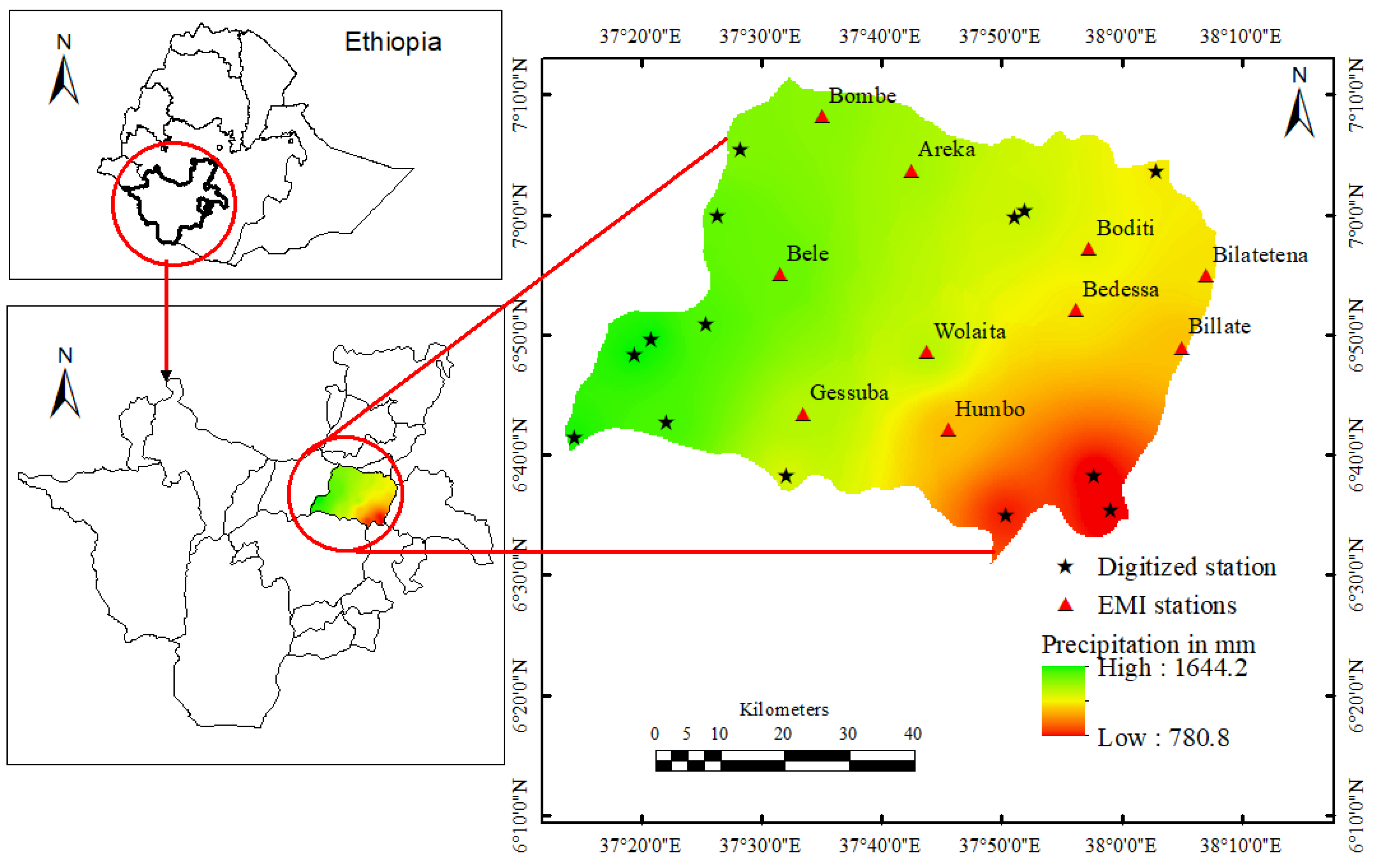
Figure 2.
Shows spatially averaged and station level monthly rainfall pattern at Bilate, Bombe and Areka stations, respectively.
Figure 2.
Shows spatially averaged and station level monthly rainfall pattern at Bilate, Bombe and Areka stations, respectively.
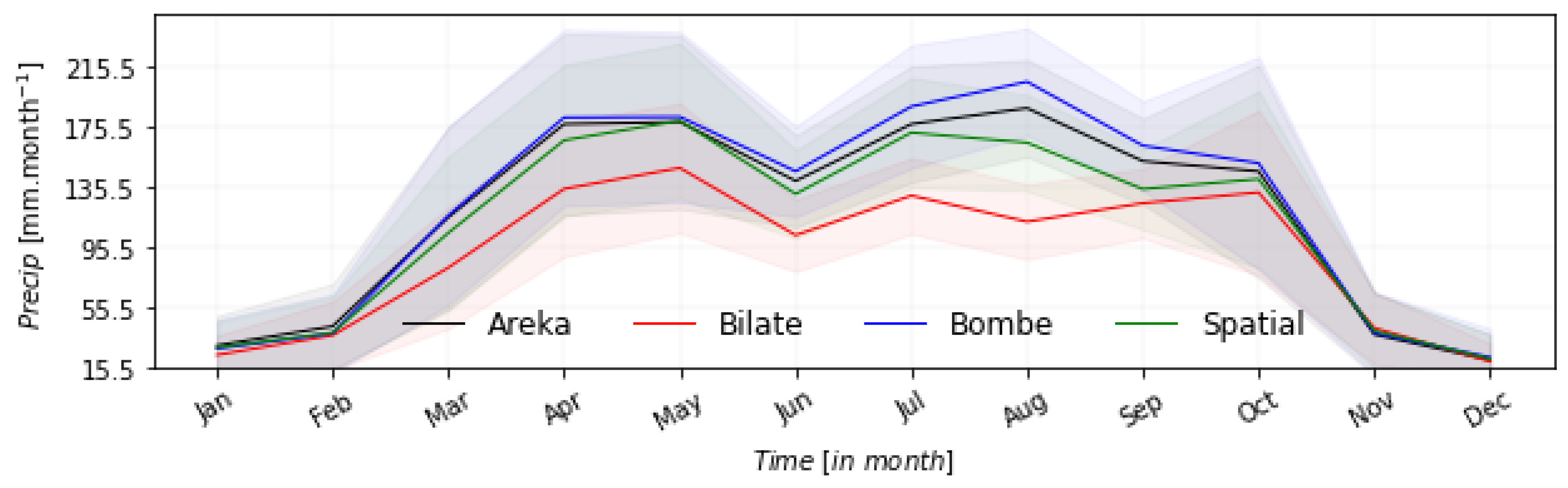
Figure 3.
Shows Coefficient of Variations in % for (a) annual rainfall, (b) Kiremt (summer) rainfall, (c) Belg (spring) rainfall and (d) Bega (autumn) rainfall, respectively.
Figure 3.
Shows Coefficient of Variations in % for (a) annual rainfall, (b) Kiremt (summer) rainfall, (c) Belg (spring) rainfall and (d) Bega (autumn) rainfall, respectively.
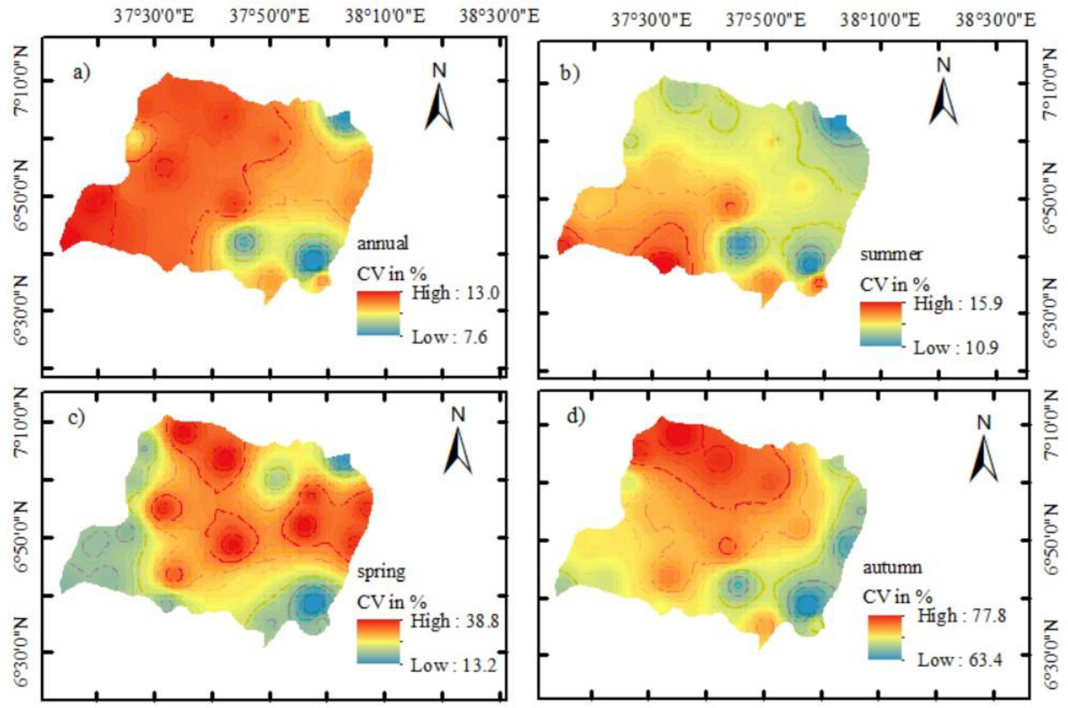
Figure 4.
Shows monthly maximum temperature (a), mean temperature (b) and minimum temperature (c) at Areka, Bilate, Bombe stations and spatially averaged over the study area.
Figure 4.
Shows monthly maximum temperature (a), mean temperature (b) and minimum temperature (c) at Areka, Bilate, Bombe stations and spatially averaged over the study area.
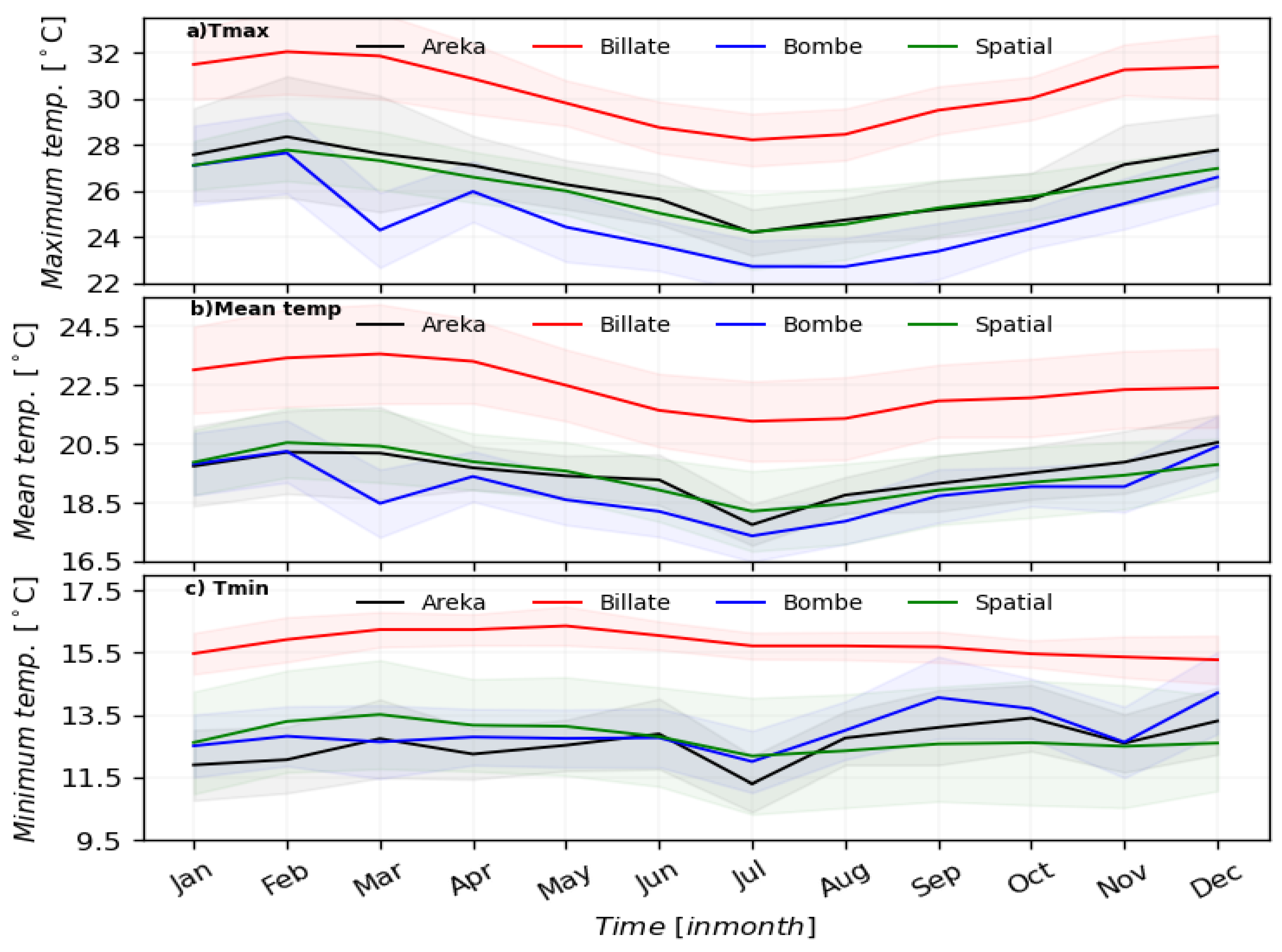
Figure 5.
Shows sweet potato (a) and taro (b) yield anomaly and trend for 2002 to 2016 period.
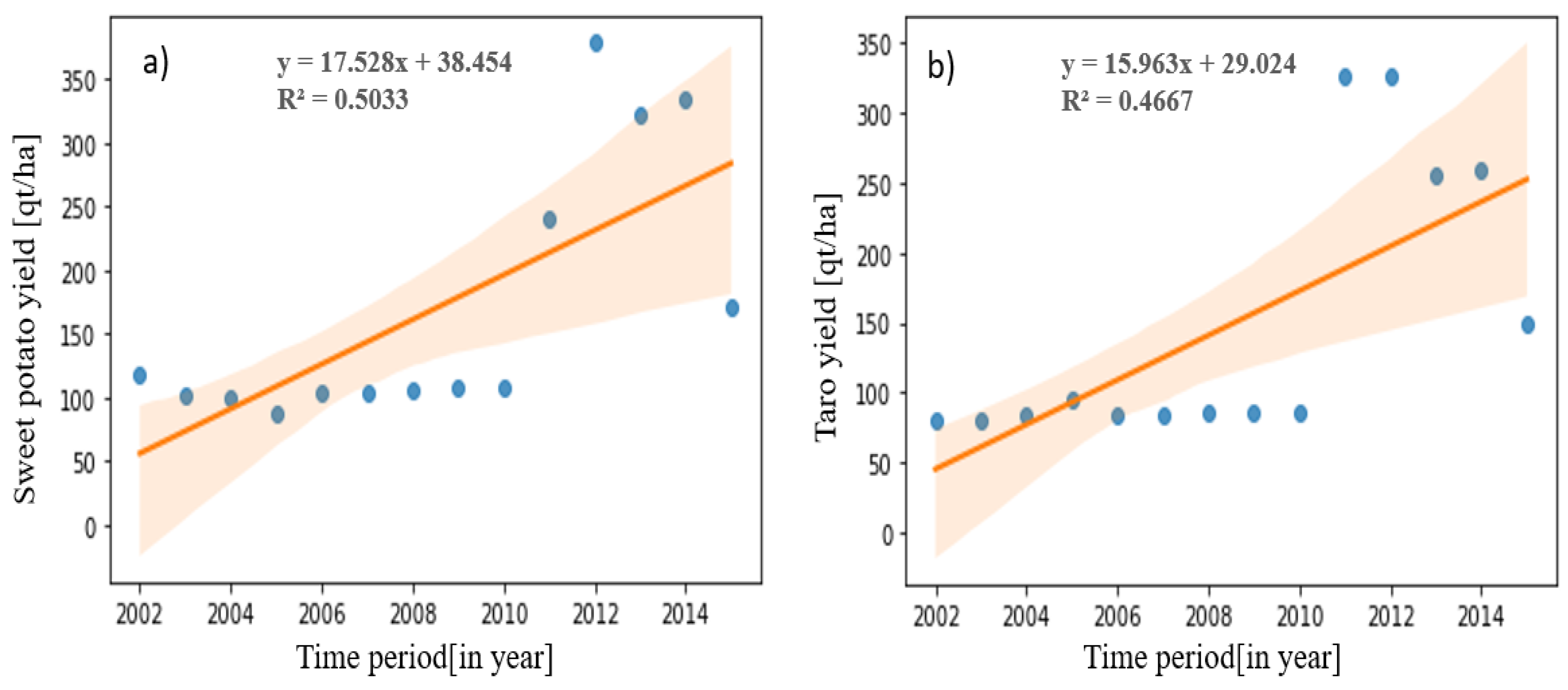
Figure 6.
Depicts Seaborne bivariate KDE between rainfall, maximum, minimum and mean temperature with sweet potato yield.
Figure 6.
Depicts Seaborne bivariate KDE between rainfall, maximum, minimum and mean temperature with sweet potato yield.
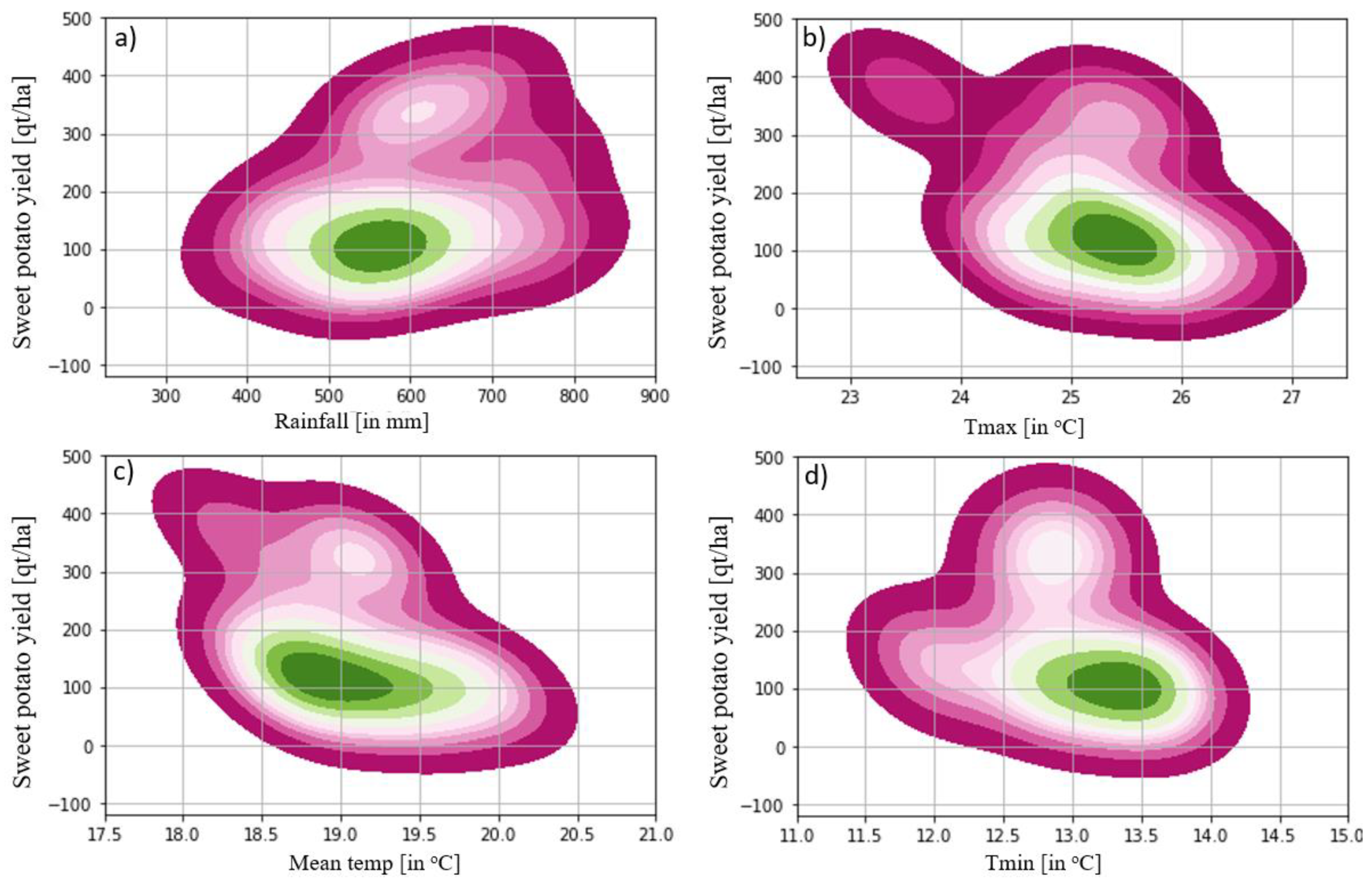
Figure 7.
Shows Seaborne bivariate KDE between rainfall, maximum, minimum and mean temperature with taro yield.
Figure 7.
Shows Seaborne bivariate KDE between rainfall, maximum, minimum and mean temperature with taro yield.
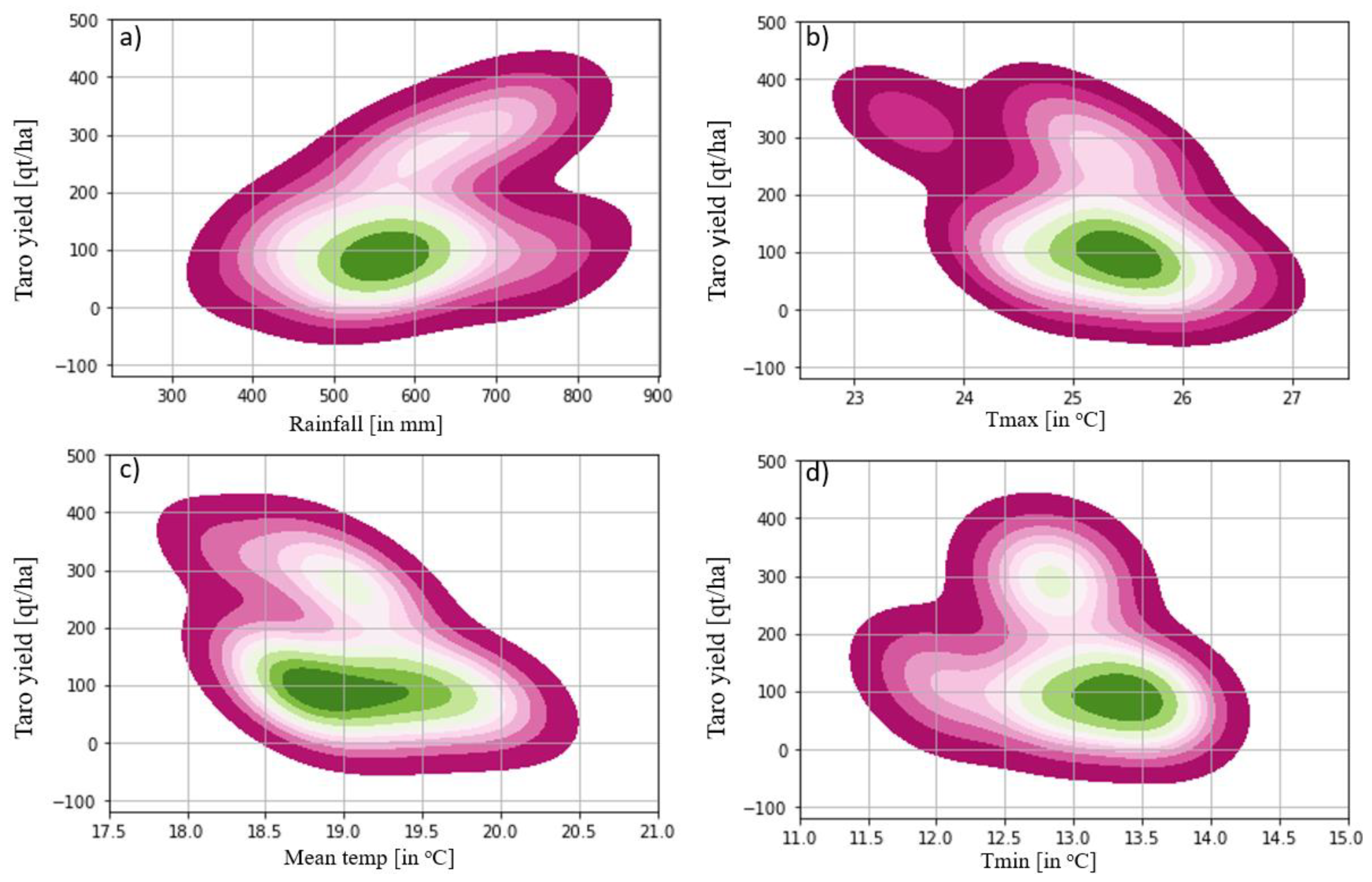

Table 1.
Present spatially averaged monthly rainfall characteristics, percent of contribution (in %), coefficient of Variation (CV in %/) , Modified Mann Kendal (MMK) trend test and Sen’s Slope (in mm) during the period of 1981 to 2021.
Table 1.
Present spatially averaged monthly rainfall characteristics, percent of contribution (in %), coefficient of Variation (CV in %/) , Modified Mann Kendal (MMK) trend test and Sen’s Slope (in mm) during the period of 1981 to 2021.
| Mon | Contribution(%) | CV (%) | MK test | Sen’s slope |
| Jan | 2.09 | 60.4 | -0.013 | -0.020 |
| Feb | 5.31 | 72.0 | + 0.18 | +1.04 |
| Mar | 7.93 | 48.7 | + 0.062 | +0.37 |
| Apr | 12.15 | 30.3 | + 0.068 | +0.59 |
| May | 13.34 | 29.7 | + 0.066 | + 0.50 |
| Jun | 9.77 | 23.4 | + 0.090 | +0.385 |
| Jul | 13.02 | 22.2 | -0.035 | -0.169 |
| Aug | 11.89 | 19.2 | -0.018 | -0.136 |
| Sep | 9.78 | 19.9 | -0.175 | -0.58 |
| Oct | 10.27 | 41.7 | +0.11 | +0.83 |
| Nov | 2.91 | 62.5 | + 0.163 | + 0.35 |
| Dec | 1.55 | 76.5 | + 0.067 | +0.07 |
Table 2.
Show seasonal and annual rainfall characteristics, Mann-Kendal (MK) trend test, Sen’s Slope (SS), percent of contribution (% cont) and coefficient of variation 1981 to 2021 period.
Table 2.
Show seasonal and annual rainfall characteristics, Mann-Kendal (MK) trend test, Sen’s Slope (SS), percent of contribution (% cont) and coefficient of variation 1981 to 2021 period.
| Parameters | Spatially averaged | Areka | Bedessa | Bele | Bilatetena | Billate | Boditi | Bombe | Gessuba | Humbo | Wolaita | |
| Annual | mean | 1324.8 | 1408.5 | 1218.1 | 1526.3 | 1214.3 | 1144.4 | 1275.0 | 1465.3 | 1376.8 | 1134.6 | 1372.5 |
| MMK | 0.119 | 0.0021 | -0.1014 | -0.001 | -0.156 | -0.114 | -0.069 | 0.0443 | -0.035 | -0.097 | 0.027 | |
| SS | +0.275 | 0.128 | -1.686 | -0.035 | -2.547 | -2.095 | -1.478 | 1.0482 | -0.761 | -0.864 | 0.615 | |
| Spring | mean | 490.7 | 236.7 | 216.0 | 270.0 | 234.2 | 228.3 | 226.1 | 243.0 | 234.7 | 209.3 | 236.4 |
| MMK | +0.106 | 0.202 | 0.141 | 0.167 | 0.107 | 0.17 | 0.133 | 0.1897 | 0.157 | -0.053 | 0.238 | |
| SS | 0.32 | 2.16** | 1.250 | 1.945 | 0.947 | 1.382 | 1.208 | 0.05** | 1.076 | -0.283 | 2.24** | |
| %cont | 35.7 | 36.6 | 37.1 | 36.4 | 37.9 | 36.9 | 37.6 | 35.5 | 36.9 | 35.7 | 35.2 | |
| Summer | mean | 602.9 | 658.8 | 551.3 | 704.3 | 521.6 | 495.4 | 570.3 | 704.9 | 637.0 | 521.9 | 654.3 |
| MMK | -0.043 | -0.019 | -0.173 | 0.024 | -0.181 | -0.11 | -0.139 | 0.087 | -0.0243 | 0.0317 | -0.056 | |
| SS | -0.455** | -0.248 | -1.576 | 0.363 | -1.284 | 0.913 | -1.235 | 0.796 | -0.178 | 0.2190 | -0.762 | |
| %cont | 47.8 | 46.8 | 45.3 | 46.1 | 42.9 | 43.3 | 44.7 | 48.1 | 46.3 | 46 | 47.7 | |
| Autumn | mean | 233.5 | 265.3 | 240.5 | 300.6 | 258.1 | 250.7 | 251.7 | 272.8 | 262.6 | 231.9 | 264.1 |
| MMK | +0.197 | 0.202 | 0.141 | 0.167 | 0.1076 | 0.170 | 0.133 | 0.189 | 0.157 | -0.053 | 0.238 | |
| SS | 1.67** | 2.18** | 1.25 | 1.945 | 0.947 | 1.382 | 1.208 | 1.49** | 1.076 | -0.28 | 2.24** | |
| % cont | 16.5 | 16.8 | 17.7 | 17.7 | 19.3 | 20 | 17.7 | 16.6 | 17 | 18.4 | 17.2 |
Table 3.
Shows annual mean, Tmax and Tmin trend for 1981-2021 period.
|
Stations |
Tmax | Mean | Tmin | |||||||||
| Mean | MMK | SS | CV | Mean | MMK | SS | CV | Mean | MMK | SS | CV | |
| Areka | 26.4 | 0.068 | 0.64 | 3.5 | 19.5 | 0.06 | 0.003 | 2.6 | 12.6 | -0.03 | -0.09 | 1.9 |
| Bedessa | 27 | 0.3 | 0.04** | 3.3 | 20.5 | 0.326 | 0.044** | 6.1 | 13.9 | 0.35 | 0.042** | 13.3 |
| Bele | 30.3 | 0.46 | 1.69** | 3.4 | 23.7 | 0.44 | 0.025** | 2.3 | 17.1 | -0.02 | -0.006 | 1.6 |
| Bilatetena | 27.7 | 0.3 | 0.033** | 3.4 | 20.4 | 0.29 | 0.038** | 5.9 | 13.1 | 0.26 | 0.037 | 12.7 |
| Billate | 30.3 | 0.23 | 0.032 | 2.9 | 22.4 | 0.302 | 0.039** | 5.6 | 14.5 | 0.26 | 0.037 | 12.8 |
| Boditi | 24.4 | 0.23 | 0.18 | 3.3 | 18.6 | 0.329 | 0.035** | 6.2 | 12.7 | 0.54 | 0.043** | 14.5 |
| Bombe | 24.8 | 0.029 | 0.001 | 1.4 | 18.5 | -0.014 | -0.006 | 1.1 | 12 | 0.05 | 0.001 | 1.9 |
| Gessuba | 29.2 | 0.28 | 0.017** | 2.4 | 21.8 | 0.251 | 0.025** | 3.3 | 14.4 | 0.097 | 0.017 | 8.3 |
| Humbo | 27.5 | 0.36 | 0.029** | 2.3 | 21.6 | 0.358 | 0.015** | 1.6 | 15.8 | -0.034 | -0.0007 | 0.9 |
| Wolaita | 25.8 | 0.23 | 0.13 | 2.6 | 19.5 | 0.173 | 0.016 | 5.1 | 13.1 | 0.031 | 0.008 | 11.9 |
| Spatial | 26.1 | 0.5 | 0.053** | 2.2 | 19.4 | 0.39 | 0.032** | 5.0 | 12.8 | 0.082 | 0.016 | 11.8 |
Table 4.
Show descriptive statistics and trend of taro and sweet potato yield, respectively.
| Parameters | MMK | SS | Mean | SD | cv | Min | Max |
| Taro | 0.46 | 6.069 | 188.28 | 103.5 | 55.0 | 85.8 | 378.7 |
| Sweet Potato | 0.516 | 5.36** | 166.40 | 89.9 | 54.0 | 80 | 327 |
Table 5.
Shows predictive potential of GBR, XGBR, RF and MLR models comparison.
| Yield | RMSE | R-squared | |
| GradientBoosting Regression | Taro | 172.2868 | 0.77599941896428238 |
| Sweet potato | 142.7695 | 0.769999976968095767 | |
| XGBRegression | Taro | 205.32352475 | 0.68999999999872404 |
| Sweet potato | 148.380 | 0.7499999998997617 | |
| RandomForest Regression | Taro | 127.2413 | 0.779352310866891 |
| Sweet potato | 117.208339 | 0.7970453256514087 | |
| Linear Regression | Taro | 96.555238 | 0.367658073611723 |
| Sweet potato | 82.21450 | 0.24159370708581318 |
Disclaimer/Publisher’s Note: The statements, opinions and data contained in all publications are solely those of the individual author(s) and contributor(s) and not of MDPI and/or the editor(s). MDPI and/or the editor(s) disclaim responsibility for any injury to people or property resulting from any ideas, methods, instructions or products referred to in the content. |
© 2025 by the authors. Licensee MDPI, Basel, Switzerland. This article is an open access article distributed under the terms and conditions of the Creative Commons Attribution (CC BY) license (http://creativecommons.org/licenses/by/4.0/).
Copyright: This open access article is published under a Creative Commons CC BY 4.0 license, which permit the free download, distribution, and reuse, provided that the author and preprint are cited in any reuse.


