
Submitted:
23 January 2025
Posted:
24 January 2025
You are already at the latest version
Abstract
A set of triaxial MEMS (Micro-Electro-Mechanical Systems) accelerometer, of commercial type, has been calibrated on a test bench, which is based on a rotating table. The bench has been designed for this specific purpose and it allows to calibrate contemporaneously all accelerometer measuring components, by realizing accurate reference accelerations in the frequency range 0 to 8 Hz. A working model of the calibration set-up and procedure is described to realize a complete and detailed uncertainty budget of the reference and of the sensor accelerations. Experimental uncertainty assessment of all the accelerometers has been carried out, allowing to obtain all the linearity and sensitivity data, accelerometer by accelerometer, axis by axis. Data processing has been carried out and interesting information is get about the level of uncertainty which is achievable, depending on the way the calibration data are evaluated, taking into account or not differences of sensitivity data for each other accelerometer and/or considering differences among measuring components of a single accelerometer.
Keywords:
Three-axis MEMS accelerometer
; multi-axis calibration
; uncertainty modelling
; uncertainty assessment
1. Introduction
MEMS technology is widely acknowledged to be able to realize sensors useful for many applications and in different engineering sectors. These devices have many interesting measuring characteristics like miniaturization, high metrological performance, digital output for easy networking and low cost [1]. In particular, MEMS accelerometers gained a relevant role thanks to the possibility of realizing triaxial accelerometers for different fields of application. For example, MEMS accelerometers are employed in aerospace, civil, automotive and automation sectors [1].
In particular, the cost-effectiveness makes them ideal for large-scale deployment in Structural Health Monitoring (SHM) applications, where many sensors are required across vast areas (e.g., bridges, entire buildings or groups of buildings). The ability to deploy many sensors increases the likelihood of detecting localized issues, providing a more comprehensive picture of the overall health of a structure [2,3,4]. The low-frequency range vibrations (typically below 100 Hz), which are often associated with the natural frequencies of structures, is of particular interest in this field [5].
More and more the number of possible applications is increased, the need to completely satisfy metrological requirements is increased too, like reproducibility and traceability. Some problems have to be highlighted with reference to this aspect, mainly due to the low cost production processes, which are not easy to keep completely under control. Furthermore, the need of low cost and digital calibration is a difficult task, since many causes of uncertainty should be considered, like zero-bias, sensitivity nonlinearity, cross-axis effect related to non-orthogonality and the crosstalk effect between different channels caused by the sensor electronics, temperature and environmental effects [6,7]. Furthermore, modelling all these causes of error is not easy for reliable estimation of uncertainty, so that a huge attention is paid to methods for calibration, which could be used in practical cases [6].
- Non- autonomous (classical) calibration: this calibration needs to be realized by means of precise devices with very good mechanical structure, such as a high-precision turntable, centrifuge, shaking table, and so on.
- Autonomous calibration: without the assistance of high-precision instruments, this calibration is completed by using the external reference excitation provided by the local gravity field, the rotational angular velocity of the earth, uniform magnetic field, and so on.
Both classes of calibration methods present advantages and disadvantages with respect to each other: in the former class the main requirement is that an accurate acceleration standard has to be realized by checking geometrical and motion characteristics but also relative positioning is important so that misalignment of the test bench with respect to the device under test is a further source of uncertainty [9,10]. Some different test benches have been realized which gave great contribution to static and dynamic calibration [11,12,13,14,15,16,17,18].
In autonomous calibration methods the gravity excitation is typically used, changing the orientation of the measuring axes of the accelerometer with respect to it and using the assumed different positions to fit the main sensitivities, the cross ones and bias, paying attention mainly to the effect of the geometrical configuration of the measuring axes and of angles between axes, which are not exactly right angles. In general, a matrix method is used to model the geometrical errors [6,19] and different algorithms are developed to improve the fitting of the data, the Allan variance [19], the Kalman Filter [20], the ellipsoid [21]; it is interesting that the reference angles with respect to the vertical direction in some cases are realized embedding the triaxial accelerometer in a multifaced device whose different positions are inclined differently with respect to the vertical without using turntable or angular encoders [22]; of course, also in this case, the geometrical accuracy of the device realizing angles of inclination of the reference device affects the uncertainty of error estimation, even though very accurate result could be achieved without any prior assumption [9]. In some cases, the matrix method is developed to make more robust the method of computation of main sensitivities and bias, by individuating outliers [23].
A merging approach, based on a rotating device, without using it as an acceleration reference, is proposed in [24]; A tilted, freely rotating bench, made of a simple wheel mounted on a static support. The accelerometer is fastened to the bench, which is then manually set into rotation; the acceleration signal is then acquired while the bench is freely rotating. No a-priori knowledge is required about the bench rotation: the proposed calibration procedure estimates both the calibration parameters and the bench motion. Only the distance of the sensor from the rotation axis needs to be known, which can be easily obtained through direct measurement on the bench. The estimation accuracy of the sensitivities depends on the noise level, being typically less than 1%, as a percentage value.
Environmental effects are also studied, in particular drift effects due to the temperature, [25] even though they are out of this analysis boundaries, which is based on calibration and traceability aspects, which are typical of a laboratory calibration.
Taking into account the previous considerations, it is to point out that many opportunities derive from the autonomous approach, even though mostly the geometrical aspects are studied and evaluated, which is an important effect but is not the whole contribution to the uncertainty budget.
An important effect to be taken into account during calibration, in particular when low cost sensors are considered, is the linearity of the MEMS transducers with reference to the whole measuring range. They are typically able to measure acceleration up to ± 10 g, therefore, using input acceleration in the range ± 1 g, it is difficult to assess linearity. Even though some efforts in this direction have been made [1,19], only using a non-autonomous approach sensor linearity could be assessed.
Based on these aspects, in this work a rotary test bench for multi-axis MEMS accelerometer calibration has been designed and tested, in order to carry on multi-axis dynamic sensitivity analysis by alternative oscillations driven by an electrical motor with a high accuracy angular encoder. Two axes of the accelerometer could be calibrated at once, set according to the tangential and radial accelerations of the table. Operating with these accelerations at the same time is considered a realistic representation of the infield working conditions. A careful model of the calibration system will be described in order to obtain a full uncertainty budget of the estimated main and cross sensitivities and information about sensor linearity. Developing a previous work of the authors [26,27,28,29], many MEMS accelerometers have been examined with the aim of highlighting the uncertainty to be assumed. Different cases are considered: evaluating the sensitivity (and its uncertainty) of the whole batch of accelerometer, studying, instead, single sensors or, finally, giving metrological specifications for each axis of each accelerometer. In section 2 the methodology will be described to build a suitable calibration uncertainty budget and the experimental program; in section 3 the results will be presented and discussed; conclusions will end the paper.
2. Materials and Methods
2.1. Devices Under Test
Eight commercial, low-power, digital, MEMS accelerometers by STMicroelectronics, which are part of the same production batch, are examined in this study. Each accelerometer is part of an inertial measurement unit (LSM6DSR model [30]), composed by an analog-to-digital converter, a charge amplifier, a 3-D accelerometer, and a 3-D gyroscope. Since only sensitivity related to acceleration is tested for the purposes of this study, the 3-D gyroscope is not used and is kept off. A serial cable connects the digital MEMS accelerometers to an external microcontroller (STMicroelectronics, model 32F769IDISCOVERY [24]). Through the use of a USB cable, this microcontroller connects to a PC to transfer the digital data acquired by the sensor. Amplitude values range between -216-1= -32768 D16-bit-signed and +(216-1-1) = +32767 D16-bit-signed, where the digit unit is a signed 16-bit sequence converted into a decimal number. The sensitivity of the digital MEMS accelerometers is expressed by the manufacturer in terms of mg/LSB (g is the gravitational acceleration and LSB means Least Significant Bit) and it depends on the “full scale” set in the testing: by using a “full scale” of ±8 g, the sensitivity declared is 0.244 mg/LSB [31], corresponding to 418 D16-bit-signed/(m/s2).
2.2. Calibration Bench
The MEMS under test are calibrated using a PLA (poly lactic acid) 3D-printed disk. It rotates around its symmetry axis, and it is mounted on the axis of a Schneider Electric servomotor. The calibration bench is represented in Figure 1.
To study all the axes, the MEMS sensors are placed on different 3D-printed supports. These are specifically made to change the MEMS orientation with respect to the tangential and centripetal accelerations, so that, in each configuration, two axes are simultaneously stressed. In particular, three supports are made to achieve the following positioning:
- X-axis parallel to the tangential acceleration and Y-Axis to the centripetal acceleration (Figure 2.a);
- Z-axis parallel to the tangential acceleration and X-Axis to the centripetal acceleration (Figure 2.b);
- Z-axis parallel to the centripetal acceleration and the Y-Axis to the tangential acceleration (Figure 2.c).
Another support is used for attaching the microcontroller on the disk.
2.3. Reference Acceleration
In this paper the reference acceleration values for calibration are obtained on the basis of the angular position of the servomotor axis, provided by the high accuracy encoder.
The Programmable Logic Controller (PLC) that allows the management of the rotating disk provides the value of the angular position of the servomotor axis over time:
In addition, the system also provides the angular speed , obtained as a derivative of :
Were
This information has been used to calculate the reference centripetal and tangential accelerations, as described in the following:
where f is the oscillation frequency, and r is the distance of the sensitive element of the accelerometer under test from the rotation axis.
The supports have been designed and installed on the disk in such a way that the center of the sensor under test (where the sensitive element is placed) is positioned at a nominal distance from the axis of rotation equal to r = 170 mm (standard uncertainty equal to 0.5 mm, in percentage 0.3%)
It should be noticed that the centripetal acceleration, as it appears in Eq. 3, is characterized by double the frequency with respect to the tangential one. This aspect must be taken into consideration and represents the main difference between the curvilinear calibration bench and the linear ones, where the axes are stressed by accelerations at the same frequency. It is also noted that the constant term in the radial acceleration is equal to the amplitude of the acceleration itself, then it could be simply obtained by averaging the signal.
In addition, a second reference IEPE accelerometer (Integrated Electronics Piezoelectric, Model TLD356B18, PCB Piezotronics, measurement range: ± 5g) has been positioned at a distance of 145 ± 0.1 mm from the rotation axis, for comparison and validation purposes.
2.4. Test Plan
The tests are carried out considering two different oscillation frequencies: 5 Hz and 8 Hz.
For each frequency, the oscillation angle is set in order to not exceed the limit value of ± 5 g, which is the maximum acceleration that can be measured using the IEPE accelerometer. Therefore, positioning the MEMS at a radius of 170 mm, the theoretical testing conditions are the following:
- Setting 5 Hz as the oscillation frequency and angle at 34°: the amplitude of the tangential acceleration is equal to 49 m/s2 and centripetal acceleration is equal to 15 m/s2;
- Setting 8 Hz as the oscillation frequency and angle at 13°: the amplitude of the tangential acceleration is equal to 49 m/s2 and centripetal acceleration is equal to 6 m/s2.
For each experimental setup, the data from the digital MEMS, the IEPE accelerometer, and the motor encoder are recorded for 40 s. Each test is repeated for 6 times.
2.5. Data Processing
2.5.1. Sensitivity Evaluation
The purpose of data processing is to evaluate the amplitude of the measured and the reference acceleration, and to make the ratio of them to determine the sensitivity of the tested accelerometer, at the oscillation frequency.
The signal from the digital MEMS and the IEPE accelerometer are filtered using a 6-pole digital low-pass Butterworth filter with a cutting frequency of 40Hz [26]. From the encoder data, the centripetal and tangential acceleration amplitudes are calculated using Eq.3 and Eq.4. A zero-crossing algorithm is applied to all the signals (from the accelerometer and the encoder) to select entire periods. This procedure is implemented to reduce the leakage during the further analysis. All the data processing steps are made using MATLAB R2023b.
As stated in previous works by the authors [26], the sampling frequency of the digital MEMS is not constant over time. Moreover, the mean value appears to not be equal to the selected one and it is not constant among different sensors. To evaluate the mean value of the sampling frequency, needed by the algorithm for the amplitude determination, the following procedure is developed.
The signal is processed using the Fast Fourier Transform (FFT) at different sampling frequencies ranging from 1560 Hz to 1760 Hz with a step of 1Hz.
Then, the mean sampling frequency is identified as the one that maximizes the amplitude at the oscillation frequency (5 Hz, or 8 Hz). The contribution to the variability of this procedure should be considered as a part of the measurement repeatability.
For tangential acceleration, the harmonic of interest corresponds to the frequency of the oscillation itself. In contrast, centripetal acceleration theoretically exhibits two significant harmonic components: the first is at twice the frequency of the oscillation, and the second is a constant component, representing the steady-state part of the centripetal acceleration (refer to Eq. 3).
Finally, for each test, the sensitivity of the tangential axis and the centripetal axis are calculated.
In Section 2.4.2 all the acceleration components will be analyzed also with respect to the effects on their uncertainty of the geometrical and operating characteristics precision, in order to set the most accurate approach.
The sensitivity values obtained are finally averaged over different groups of values, in order to investigate the possibility of assuming:
- A unique sensitivity value. This is supposed independently of the accelerometer, of the measuring axis and of the way the sensitivity is evaluated. This is the most general and easy approach for in-field use; however, it is important to estimate the uncertainty of the method;
- A single value of sensitivity for each accelerometer, common for all the three measuring axes;
- Specialize the sensitivity indication to the single axis of the single accelerometer. This approach seems to be the most accurate, even though much data must be acquired before the accelerometer can be used.
2.6. Uncertainty Evaluation
For the evaluation of the uncertainty of the sensitivity, the repeatability, linearity, and uncertainty of the reference contributions are considered.
2.6.1. Repeatability
The repeatability contribution to the uncertainty is assessed performing six repeated measures for each experimental setup. The sensitivity is calculated for each test and the repeatability contribution (ur, expressed in percentage terms) is evaluated as the standard deviation between the calculated sensitivities, according to a Gaussian probability distribution.
2.6.2. Linearity
Sensors linearity is assessed considering the output data of each sensor’s axis under different acceleration stresses. In fact, as expressed in the previous section, in the tests the acceleration amplitudes vary from the theoretical lowest value of 4 m/s2 to a maximum of about 50 m/s2. To assess the linearity uncertainty, the data regression straight line to model the relationship between the MEMS output value and the encoder reference accelerations, is calculated using the least square error method:
Where, is the output value of the MEMS accelerometer [D16-bit-signed] is the reference acceleration [m/s2], b is the intercept, and is the slope of the line [D16-bit-signed/(m/s2)], that is the sensitivity. According to [32], the standard deviation of the sensitivity can be calculated as follows:
Where
Then, can be considered as linearity uncertainty contribution of the sensitivity S, expressed in percentage terms.
2.6.2. Uncertainty of the Reference
The uncertainty of the reference depends on the uncertainty of the encoder, which is very low (0.01°), and also on the agreement between the movement actually performed and the theoretical sinusoidal one.
To estimate the quality of the reference, some preliminary evaluations are carried out:
- Calculation of the repeatability of the measured amplitude of the reference acceleration, in repeated tests;
- Check that the amplitude of the angular position signal is equal to the set oscillation angle, and that the amplitude of the angular velocity signal is equal to the amplitude of the position signal, multiplied by the pulsation (as occurs in perfectly sinusoidal signals);
- Comparison with the IEPE accelerometer described in Section 2.3.
The main source of uncertainty in the reference, however, is represented by geometric imperfections of the test bench, due to the inclination of the rotation axis with respect to the vertical axis, and to the deviations in the position of the MEMS accelerometer under test with respect to the theoretical position: the latter is characterized by a distance of the sensing element from the rotation axis r = 170 mm, and two of the accelerometer axes in the radial and tangential directions, respectively. Eqs. 3 and 4, which allow to calculate the reference accelerations, in fact, presuppose a perfect positioning of the MEMS, which in reality is not possible.
An analytical model has been built to evaluate the reference uncertainty contribution due to the geometric imperfections of the bench. The parameters used in the model are shown in Figure 3, and described in Table 1. The “reference side” is the direction from which angle δ is measured clockwise, and correspond to the direction of maximum slope of the disc.
As an example, in Figure 3.b, the x-axis is in the radial direction and the y-axis is in the tangential direction; however, the experimental tests were conducted by positioning each MEMS accelerometer in such a way that the measurement axes were oriented both in the radial and tangential directions.
It must be considered that the Δs displacement produces a variation of the radius at which the sensitive element is placed, as well as a rotation of the accelerometer around its own axis: for this reason, at Step 2 of the procedure, r and β are redefined as indicated in the diagram itself.
The model has been applied assuming a maximum value of 1° for α, of 0.5° for β, and of 1 mm for Δs. This choice, in the tests at 5 Hz, involves a 5 Hz component in the radial direction not exceeding 0.15 m/s2: in the experimental tests, in fact, the correct positioning of the accelerometer has been always checked, precisely by verifying that this component did not exceed 0.15 m/s2.
The largest deviations from the ideal case (test bench without geometric imperfections) result to be of the order of 1.2% for the constant acceleration component of the axis in the radial direction, while negligible deviations (less than or equal to 0.06%) occur for the components at other frequencies, in the radial and tangential direction. This result leads to excluding the indication from null frequency in the following analysis.
3. Results
The results of the experimental activity have been examined in order to estimate the following elements:
- Metrological characteristics of the MEMS accelerometers;
- Differences among accelerometers, in order to check the opportunity of using different data depending on the behavior of the single sensor;
- Differences among indicators
3.1. Metrological Characteristics
The metrological characteristics of the MEMS accelerometers are repeatability, linearity, and sensitivity. The first indicator to be examined in order to assess the quality of the experimental data is the repeatability of data to be used for linearity and sensitivity analysis, with reference to each axial component of all accelerometers. Moreover, repeatability and linearity, together with the uncertainty due to geometric imperfections of the bench and the uncertainty of the reference, contribute to the total uncertainty.
3.1.1. Repeatability
For each experimental setup the acquisitions are repeated six times to evaluate the repeatability of the sensitivity measurements. This is calculated for each accelerometer axis stressed by the accelerations at different frequencies and amplitudes. Analyzing the tests data, the mean repeatability is in the order of 0.05 %. This result also provides an indication of the quality of the procedure used for the compensation of the sampling frequency variability.
3.1.2. Linearity
To assess the sensors linearity both the data of tangential and centripetal accelerations are used. As shown in Figure 5, there are no significant differences in linearity among the three axes of the accelerometer. In addition to this, no noticeable biases are found. According to the procedure described in Section 2.4.2, the calculation of ul leads to values less than 0.05%.
3.1.3. Uncertainty of the Reference
The repeated tests that have been carried out on the acceleration reference, according to Section 2.4.2, highlight an almost perfect repeatability (very negligible standard deviation).
Furthermore, the comparison between theoretical (sinusoidal) and real signal shows differences less than 1 ‰ in terms of instantaneous amplitude of acceleration.
In addition, the acceleration data from the encoder and that provided by the IEPE sensor, used for validation purposes, have been found to be statistically compatible [27].
Instead, the reference uncertainties due to the imperfections of the bench have been evaluated according to the procedure described in Section 2.4.2. Considering an oscillation frequency of 5 Hz, deviations less than or equal to 0.06% occur for the components at 5 and 10 Hz, in the tangential and radial direction, respectively. If a rectangular distribution is considered, the maximum uncertainty contribution, as a standard deviation, is (), that is negligible.
Therefore, considering also the uncertainty of the radius r (u_r=0.3%), the uncertainty of the reference is estimated equal to:
3.1.4. Budget for the Calibration Uncertainty Assessment
The overall uncertainty of the sensitivity, evaluated using the described rotating calibration bench, is obtained by combining all the above described contributions, and is equal to 0.9%. Table 2 shows the uncertainty budget.
3.1. Sensitivity Obtained over Grups of Data, and Corresponding Uncertainty
As said in the methodological Section, the sensitivity values obtained in the test of each accelerometer are averaged over different groups of data, to investigate the possibility of assuming, for all the accelerometers of a batch, a single sensitivity value, and evaluate what this entails in terms of uncertainty with respect to the case of calibration of each sensor. This last approach would, of course, be the most accurate, but it is not feasible in practice.
This analysis required the following steps of evaluation:
- Assessment of the mean sensitivity for each axis and each accelerometer;
- Assessment of the mean sensitivity for each accelerometer;
- Assessment of the mean sensitivity over all axes and accelerometers.
3.2.1. Assessment of the Mean Sensitivity for Each Axis and Accelerometer
Figure 6 shows the sensitivity values obtained as average for each axis and each accelerometer. The uncertainty, represented as “error bar”, is obtained combining the calibration uncertainty (0.3%) with the standard deviation of the sensitivity results obtained for each axis and each accelerometer: in average, the overall uncertainty is equal to 0.8%, 0.6%, and 0.7%, for X-, Y-, and Z- axis, respectively.
3.2.2. Assessment of the Mean Sensitivity for Each Accelerometer
Figure 7 reports the sensitivity values for each accelerometer independently to the axis. The sensitivity of each accelerometer is computed as the mean value with respect to all the axes. The sensitivity values range from 421.5 to 426.6 D16 bit-signed/(m/s2). The uncertainty is obtained as a combination of the variability of the first case and the variability among axes: on average this overall uncertainty is 0.9%.
3.2.3. Assessment of the Mean Sensitivity over all Axes and Accelerometers
Finally, considering a unique sensitivity mean value for all accelerometers, this is estimated to be equal to 423.0 D16 bit-signed/(m/s2) (Figure 8). In this case, the uncertainty is obtained as a combination of the variability of the previous case and the variability among MEMSs, and it results equal to 1%.
It should be noticed that giving a single value is the approach followed by the manufacturer. In fact, in the sensor datasheet [30] the provided sensitivity value at component level is 418 D16 bit-signed/(m/s2). However, this do not have an uncertainty budget nor a traceability statement.
Table 3 synthetizes these overall uncertainty estimates. If a single sensitivity value for all the accelerometers of the batch is provided, determined on a single axis of a single accelerometer, then the uncertainty of Case 3 should be considered: it results to be, as expected, higher than the other cases.
3.3. Sensitivity Obtained over Grups of Data, and Corresponding Uncertainty
The estimation of each axial sensitivity has been carried out by making measurements of both tangential and centripetal acceleration, but also considering vertical data, which are related to measurement of the gravity acceleration.
Tangential measurements are in general affected by less variability than radial ones when both mean or periodical values are considered (at two times the oscillation frequency). This evidence could be explained considering the accelerations amplitudes. Tangential accelerations have higher amplitudes compared to radial ones therefore, the signal to noise ratio is better. In addition to this, the misalignment effects of the test bench are reduced. As far as the constant component of the radial acceleration, this can also be used to evaluate the sensitivity of the accelerometers. Nonetheless, it is more influenced by geometrical imperfections of the oscillating disk and constant offsets are present.
As a final remark, it is to highlight that the evaluated sensitivity of all the axes of the all the accelerometers is higher than the nominal one, indicating that a promising way to use the calibration data is to correct the sensitivity data according to the calibration results, using a common value for the sensitivity itself for all the accelerometers, with an extended uncertainty of about 2% (at 95% of confidence level); if this level of uncertainty is acceptable, also the calibration uncertainty contribution and the effect of positioning of the transducer on the table is acceptable too.
The average for each accelerometer axis allows to reduce the variability, and can be evaluated if a lower level of uncertainty is required.
4. Discussion
The estimation of each axial sensitivity has been carried out by making measurements of both tangential and centripetal acceleration, but also considering vertical data, which are related to measurement of the gravity acceleration.
Tangential measurements are in general affected by less variability than radial ones when both mean or periodical values are considered (at two times the oscillation frequency). This evidence could be explained considering the accelerations amplitudes. Tangential accelerations have higher amplitudes compared to radial ones therefore, the signal to noise ratio is better. In addition to this, the misalignment effects of the test bench are reduced. As far as the constant component of the radial acceleration, this can also be used to evaluate the sensitivity of the accelerometers. Nonetheless, it is more influenced by geometrical imperfections of the oscillating disk and constant offsets are present.
As a final remark, it is to highlight that the evaluated sensitivity of all the axes of the all the accelerometers is higher than the nominal one, indicating that a promising way to use the calibration data is to correct the sensitivity data according to the calibration results, using a common value for the sensitivity itself for all the accelerometers, with an extended uncertainty of about 2% (at 95% of confidence level); if this level of uncertainty is acceptable, also the calibration uncertainty contribution and the effect of positioning of the transducer on the table is acceptable too.
The average for each accelerometer axis allows to reduce the variability, and can be evaluated if a lower level of uncertainty is required.
5. Conclusions
In this work a rotary test bench for three-axis MEMS accelerometer calibration has been used, in order to carry out a dynamic sensitivity analysis of a set of sensors from the same production batch.
The main results can be synthetized as follows:
- Differences among accelerometers and among axes of the same accelerometer are not significant from a statistical point of view, considering the variability;
- Tangential measurements are in general affected by less variability than radial ones, due to the higher amplitudes;
- The constant component of the radial acceleration could be used to evaluate the sensitivity of the accelerometers. However, it is more influenced by geometrical imperfections of the bench and constant offsets are present;
- The evaluated sensitivity of all the accelerometers’ axes is greater than the nominal one.
In the light of the results, a possible practical approach to the problem could be to evaluate the sensitivity using a limited set of accelerometers from the batch to be analysed on the proposed calibration bench, and considering a unique value for the sensitivity itself for all the accelerometers, with an extended uncertainty of about 2% (at 95% confidence level). If a lower level of uncertainty is required, the analysis of each accelerometer and each axis allows to reduce the variability.
As a final remark, it is important to notice that environmental effects are not included, in particular drift effects due to the temperature, being this work focused on calibration and traceability aspects, which are typical of a laboratory calibration.
Author Contributions
Conceptualization, G.D., L.C, A.G. and E.N.; methodology, A.G., L.C and E.N.; software, L.C.; validation, L.C. and E.N.; formal analysis, L.C. and E.N.; investigation, L.C.; resources, G.D.; data curation, L.C.; writing—original draft preparation, L.C, G.D and E.N.; writing—review and editing, A.G. and E.N.; visualization, A.G., L.C. and E.N.; supervision, G.D.; project administration, G.D.; funding acquisition, G.D. All authors have read and agreed to the published version of the manuscript
Funding
This research received no external funding
Institutional Review Board Statement
Not applicable
Informed Consent Statement
Not applicable
Data Availability Statement
The original contributions presented in the study are included in the article, and further inquiries can be directed to the corresponding authors.
Conflicts of Interest
The authors declare no conflicts of interest.
Abbreviations
The following abbreviations are used in this manuscript:
| MEMS | Micro-Electro-Mechanical Systems |
| SHM | Structural Health Monitoring |
| PLA | Poly Lactic Acid |
| PLC | Programmable Logic Controller |
| IEPE | Integrated Electronics Piezoelectric |
| FFT | Fast Fourier Transform |
References
- Babatain, W.; Bhattacharjee, S.; Hussain, A.M.; Hussain, M.M. Acceleration Sensors: Sensing Mechanisms, Emerging Fabrication Strategies, Materials, and Applications. ACS Appl. Electron. Mater. 2021, 3, 504–531. [Google Scholar] [CrossRef]
- Ragam, P.; Devidas Sahebraoji, N. Application of MEMS-Based Accelerometer Wireless Sensor Systems for Monitoring of Blast-Induced Ground Vibration and Structural Health: A Review. IET Wireless Sensor Systems 2019, 9, 103–109. [Google Scholar] [CrossRef]
- Parisi, E.; Moallemi, A.; Barchi, F.; Bartolini, A.; Brunelli, D.; Buratti, N.; Acquaviva, A. Time and Frequency Domain Assessment of Low-Power MEMS Accelerometers for Structural Health Monitoring. In Proceedings of the 2022 IEEE International Workshop on Metrology for Industry 4.0 & IoT (MetroInd4.0&IoT); June 2022; pp. 234–239.
- Komarizadehasl, S.; Lozano, F.; Lozano-Galant, J.A.; Ramos, G.; Turmo, J. Low-Cost Wireless Structural Health Monitoring of Bridges. Sensors 2022, 22, 5725. [Google Scholar] [CrossRef] [PubMed]
- Zonzini, F.; Malatesta, M.M.; Bogomolov, D.; Testoni, N.; Marchi, L.D.; Marzani, A. Heterogeneous Sensor-Network for Vibration-Based SHM. In Proceedings of the 2019 IEEE International Symposium on Measurements & Networking (M&N); July 2019; pp. 1–5.
- Ru, X.; Gu, N.; Shang, H.; Zhang, H. MEMS Inertial Sensor Calibration Technology: Current Status and Future Trends. Micromachines 2022, 13, 879. [Google Scholar] [CrossRef] [PubMed]
- Dürr, O.; Fan, P.-Y.; Yin, Z.-X. Bayesian Calibration of MEMS Accelerometers. IEEE Sensors Journal 2023, 23, 13319–13326. [Google Scholar] [CrossRef]
- Harindranath, A.; Arora, M. A Systematic Review of User - Conducted Calibration Methods for MEMS-Based IMUs. Measurement 2024, 225, 114001. [Google Scholar] [CrossRef]
- Gheorghe, M.V.; Bodea, M.C.; Dobrescu, L. Calibration of Skew Redundant Sensor Configurations in the Presence of Field Alignment Errors. IEEE Transactions on Instrumentation and Measurement 2020, 69, 1794–1804. [Google Scholar] [CrossRef]
- Gaitan, M.; López Bautista, I.M.; Geist, J. Reduction of Calibration Uncertainty Due to Mounting of Three-Axis Accelerometers Using the Intrinsic Properties Model. Metrologia 2021, 58, 035006. [Google Scholar] [CrossRef]
- Iqbal, A.; Mian, N.S.; Longstaff, A.; Fletcher, S. Performance Evaluation of Low-Cost Vibration Sensors in Industrial IoT Applications. International Journal of Automation Technology 2022, 16, 329–339. [Google Scholar] [CrossRef]
- Gaitan, M.; Geist, J. Calibration of Triaxial Accelerometers by Constant Rotation Rate in the Gravitational Field. Measurement 2022, 189, 110528. [Google Scholar] [CrossRef]
- D’Emilia, G.; Gaspari, A.; Natale, E. Amplitude–Phase Calibration of Tri-Axial Accelerometers in the Low-Frequency Range by a LDV. Journal of Sensors and Sensor Systems 2019, 8, 223–231. [Google Scholar] [CrossRef]
- Guan, W.; Meng, X.; Dong, X. Calibration of Accelerometer with Multicomponent Inputs. In Proceedings of the 2014 IEEE International Instrumentation and Measurement Technology Conference (I2MTC) Proceedings; May 2014; pp. 16–19.
- Rossi, A.; Bocchetta, G.; Botta, F.; Scorza, A. Accuracy Characterization of a MEMS Accelerometer for Vibration Monitoring in a Rotating Framework. Applied Sciences 2023, 13, 5070. [Google Scholar] [CrossRef]
- Seeger, B.; Jugo, E.; Bosnjakovic, A.; Ruiz, S.; Bruns, T. Comparison in Dynamic Primary Calibration of Digital-Output Accelerometer between CEM and PTB. Metrologia 2022, 59, 035002. [Google Scholar] [CrossRef]
- Jonscher, C.; Hofmeister, B.; Grießmann, T.; Rolfes, R. Very Low Frequency IEPE Accelerometer Calibration and Application to a Wind Energy Structure. Wind Energy Science 2022, 7, 1053–1067. [Google Scholar] [CrossRef]
- Zhang, W.; Teng, F.; Zhang, Z. Sensitivity Matrix Calibration of Triaxial High-G Accelerometer Based on Triaxial Shock Calibration Device. IEEE Sensors Journal 2024, 24, 10975–10982. [Google Scholar] [CrossRef]
- Aydemir, G.A.; Saranlı, A. Characterization and Calibration of MEMS Inertial Sensors for State and Parameter Estimation Applications. Measurement 2012, 45, 1210–1225. [Google Scholar] [CrossRef]
- Beravs, T.; Podobnik, J.; Munih, M. Three-Axial Accelerometer Calibration Using Kalman Filter Covariance Matrix for Online Estimation of Optimal Sensor Orientation. IEEE Transactions on Instrumentation and Measurement 2012, 61, 2501–2511. [Google Scholar] [CrossRef]
- Gheorghe, M.V. Advanced Calibration Method for 3-Axis MEMS Accelerometers. In Proceedings of the 2016 International Semiconductor Conference (CAS); October 2016; pp. 81–84. [Google Scholar]
- Xu, T.; Xu, X.; Xu, D.; Zhao, H. A Novel Calibration Method Using Six Positions for MEMS Triaxial Accelerometer. IEEE Transactions on Instrumentation and Measurement 2021, 70, 1–11. [Google Scholar] [CrossRef]
- Belkhouche, F. Robust Calibration of MEMS Accelerometers in the Presence of Outliers. IEEE Sensors Journal 2022, 22, 9500–9508. [Google Scholar] [CrossRef]
- Pedersini, F. Dynamic Calibration of Triaxial Accelerometers With Simple Setup. IEEE Sensors Journal 2022, 22, 9665–9674. [Google Scholar] [CrossRef]
- Giomi, E.; Fanucci, L.; Rocchi, A. New Low-Cost Concept for Characterization of MEMS Accelerometers at Medium-g Levels for Automotive. In Proceedings of the 5th IEEE International Workshop on Advances in Sensors and Interfaces IWASI; June 2013; pp. 168–173.
- D’Emilia, G.; Gaspari, A.; Natale, E.; Prato, A.; Mazzoleni, F.; Schiavi, A. Managing the Sampling Rate Variability of Digital MEMS Accelerometers in Dynamic Calibration. In Proceedings of the 2021 IEEE International Workshop on Metrology for Industry 4.0 & IoT (MetroInd4.0&IoT); June 2021; pp. 687–692.
- Chiominto, L.; D’Emilia, G.; Natale, E.; Prato, A.; Schiavi, A. Comparison between References in a Rotating Calibration Bench for Accelerometers. In Proceedings of the 2024 IEEE International Workshop on Metrology for Industry 4.0 & IoT (MetroInd4.0 & IoT); May 2024; pp. 145–149.
- D’Emilia, G.; Gaspari, A.; Natale, E. Calibration Test Bench for Three-Axis Accelerometers An Accurate and Low-Cost Proposal. In Proceedings of the 2018 IEEE International Instrumentation and Measurement Technology Conference (I2MTC); May 2018; pp. 1–6.
- Chiominto, L.; Natale, E.; D’Emilia, G.; Grieco, S.A.; Prato, A.; Facello, A.; Schiavi, A. Responsiveness and Precision of Digital IMUs under Linear and Curvilinear Motion Conditions for Local Navigation and Positioning in Advanced Smart Mobility. Micromachines 2024, 15, 727. [Google Scholar] [CrossRef]
- iNEMO Inertial Module: Always-On 3D Accelerometer and 3D Gyroscope. Available online: https://www.st.com/resource/en/datasheet/lsm6dsr.pdf (accessed on 22 January 2025).
- iNemo Inertial Module Kit Based on ISM330DHCX. Available online: https://www.st.com/en/evaluation-tools/steval-mki210v1k.html (accessed on 22 January 2025).
- Doebelin, E.O.; Manik, D.N. Measurement Systems: Application and Design. 2007.
Figure 1.
Picture of the calibration bench (a) and scheme representing the rotation test bench functioning.
Figure 1.
Picture of the calibration bench (a) and scheme representing the rotation test bench functioning.
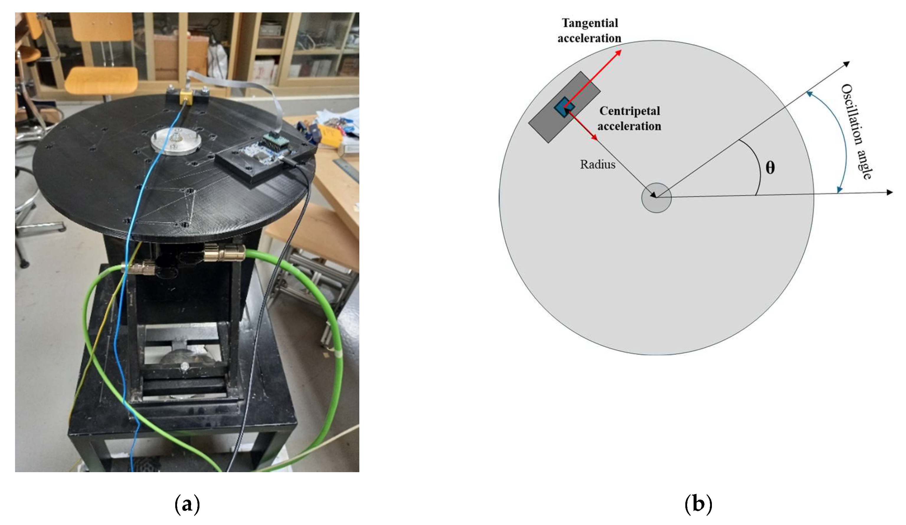
Figure 2.
Pictures of the support used to orient the MEMS axes on different positions with respect to the tangential and the centripetal accelerations.
Figure 2.
Pictures of the support used to orient the MEMS axes on different positions with respect to the tangential and the centripetal accelerations.
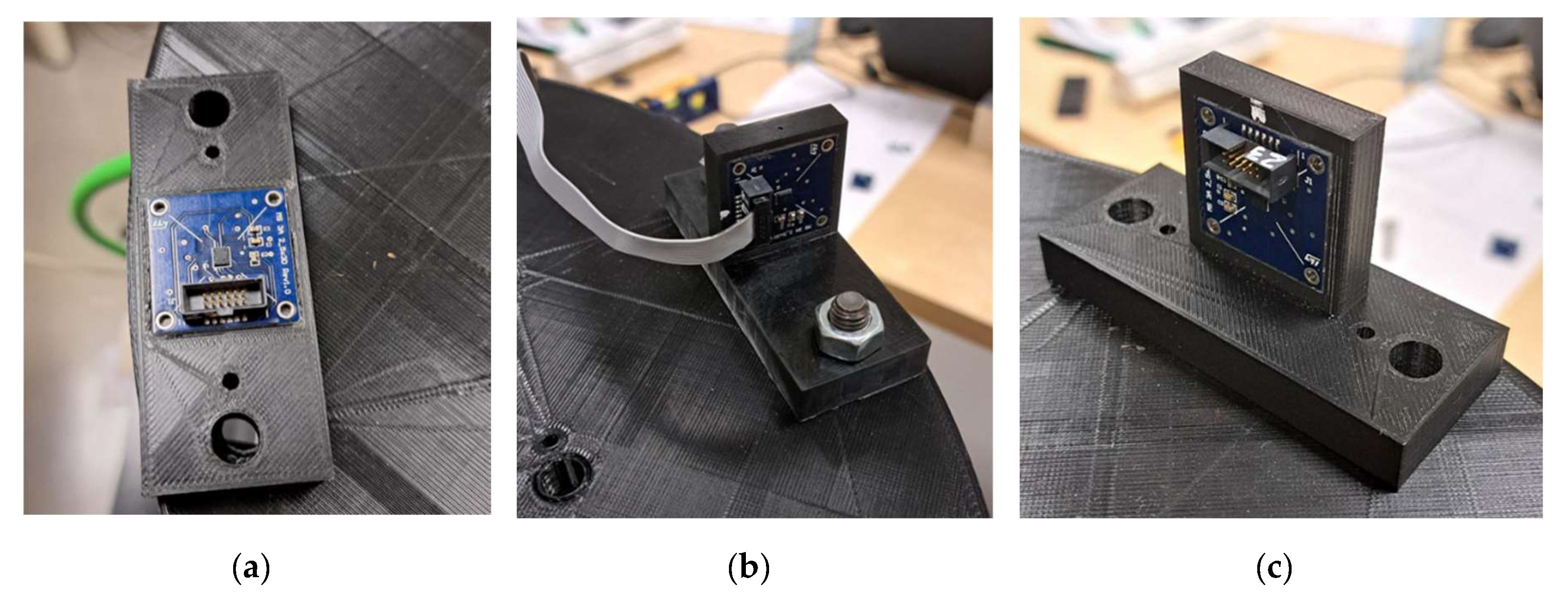
Figure 3.
Scheme of the test bench: a) lateral view; b) top view. The indication of x-y-z axis refer to the measuring reference systems.
Figure 3.
Scheme of the test bench: a) lateral view; b) top view. The indication of x-y-z axis refer to the measuring reference systems.
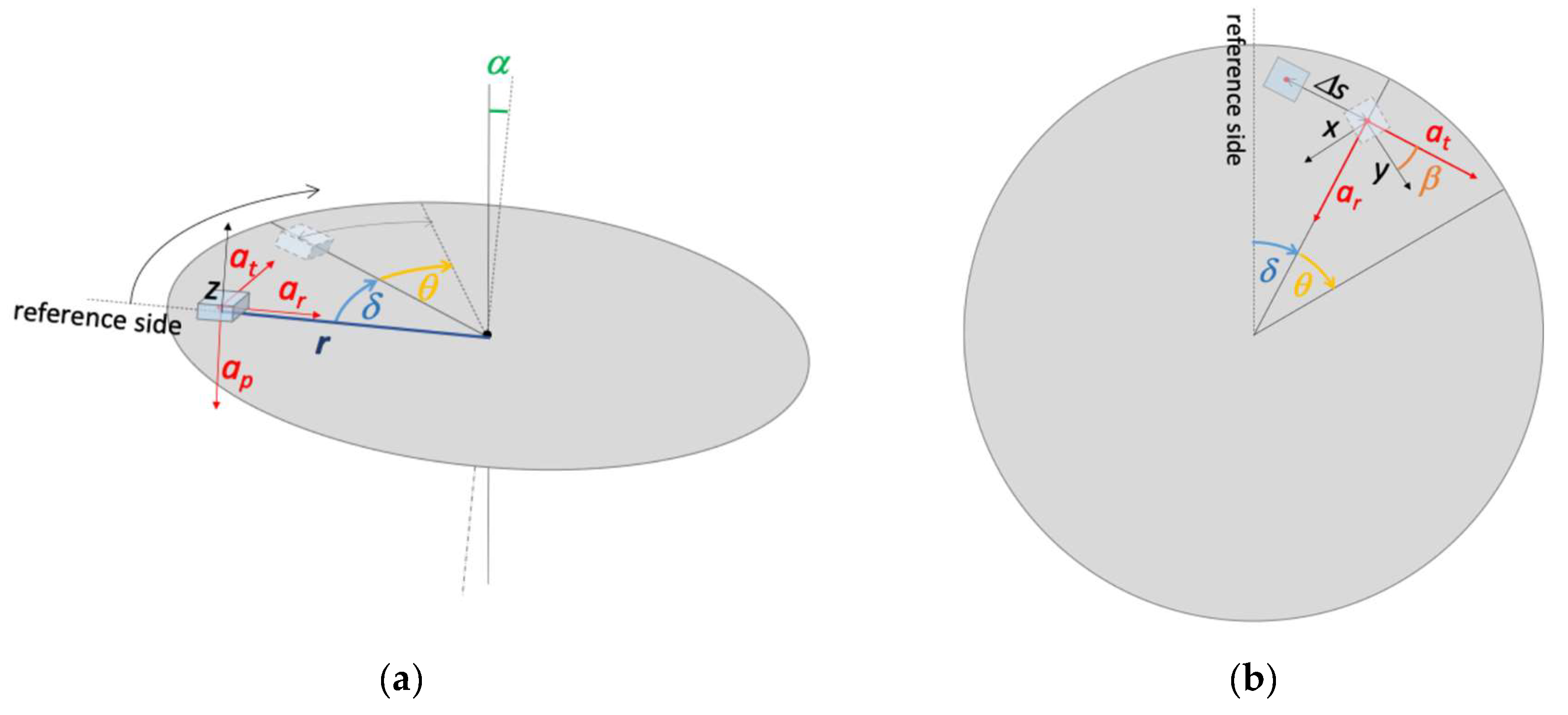
Figure 4.
Diagram of the procedure for the evaluation of the uncertainty contribution due to geometrical imperfections of the bench.
Figure 4.
Diagram of the procedure for the evaluation of the uncertainty contribution due to geometrical imperfections of the bench.
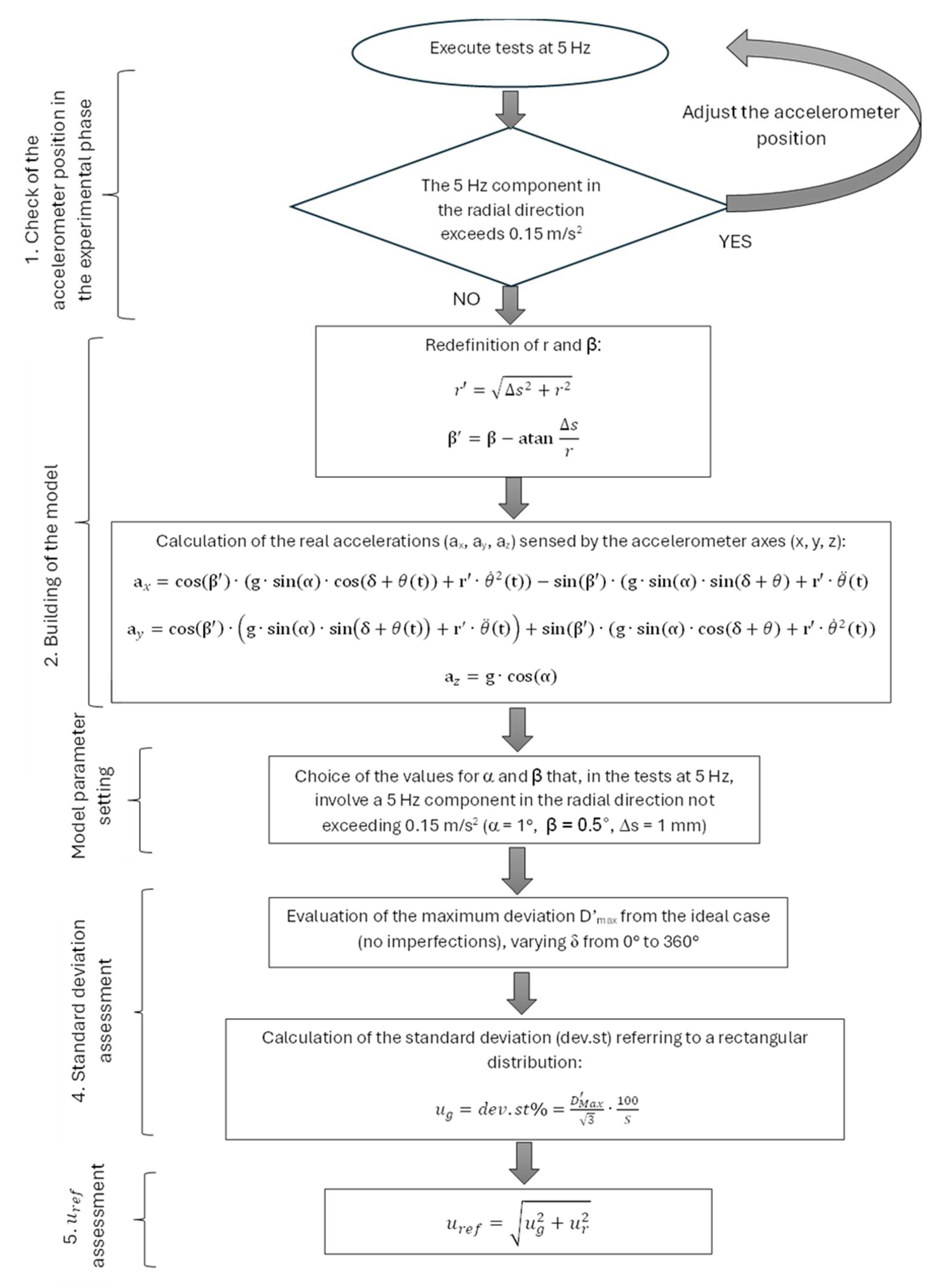
Figure 5.
Linearity of the X-axis (a), Y-axis (b), and Z-axis (c) of one of the MEMS accelerometers. The reference comes from the encoder signal.
Figure 5.
Linearity of the X-axis (a), Y-axis (b), and Z-axis (c) of one of the MEMS accelerometers. The reference comes from the encoder signal.
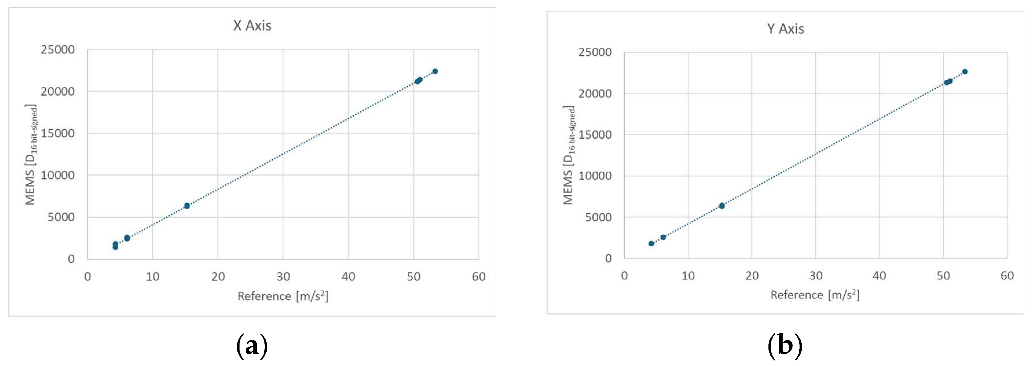
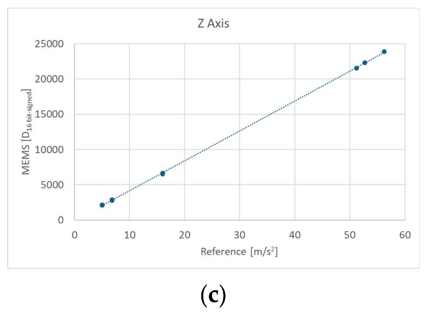
Figure 6.
Evaluated sensitivity values for each axis of each accelerometer.

Figure 7.
Evaluated sensitivities of all the studied MEMS considering a single value for each accelerometer.
Figure 7.
Evaluated sensitivities of all the studied MEMS considering a single value for each accelerometer.
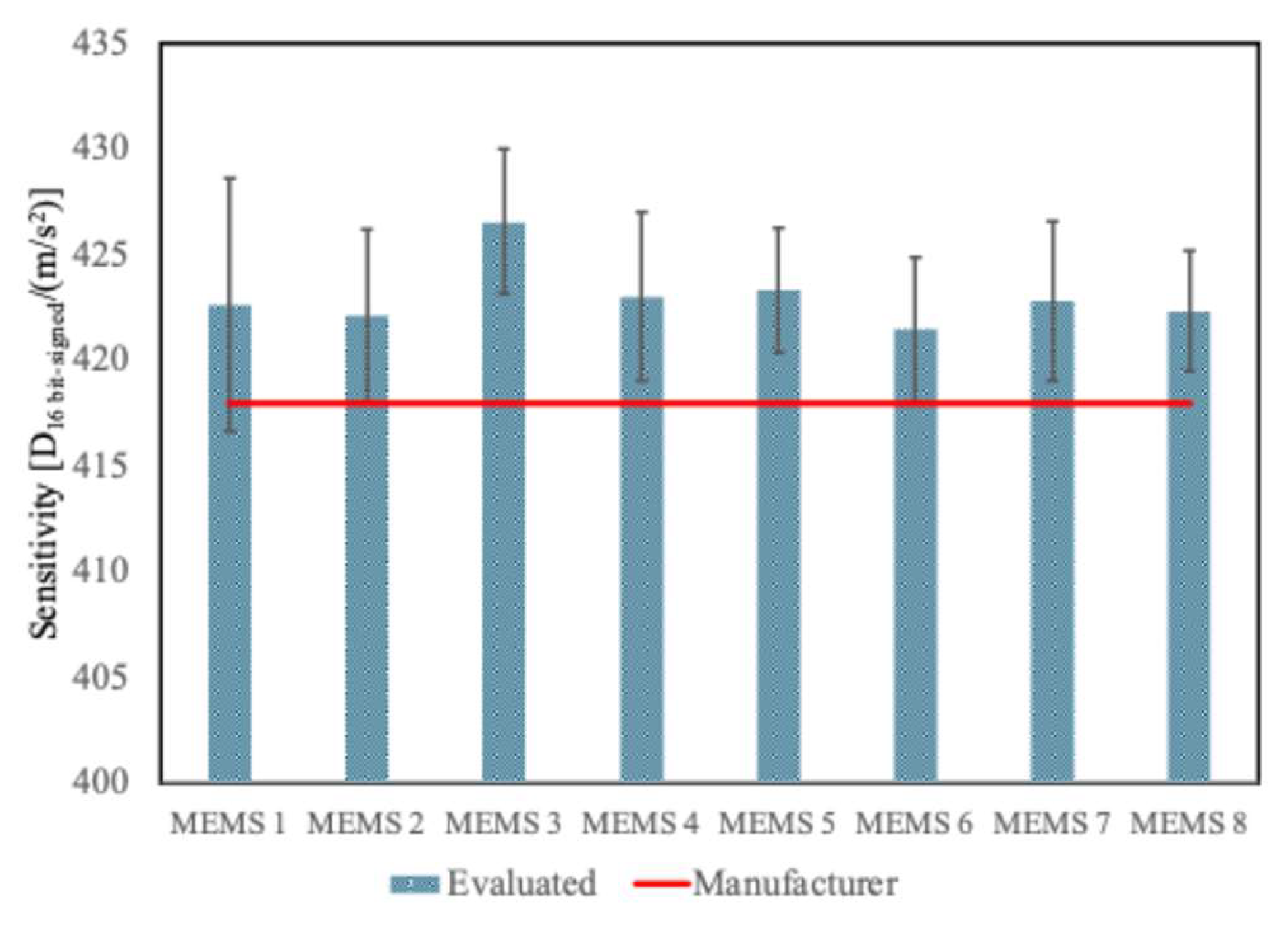
Figure 8.
Evaluated single sensitivity value for all MEMS independently of the axis or sensor compared to the manufacturer provided one.
Figure 8.
Evaluated single sensitivity value for all MEMS independently of the axis or sensor compared to the manufacturer provided one.
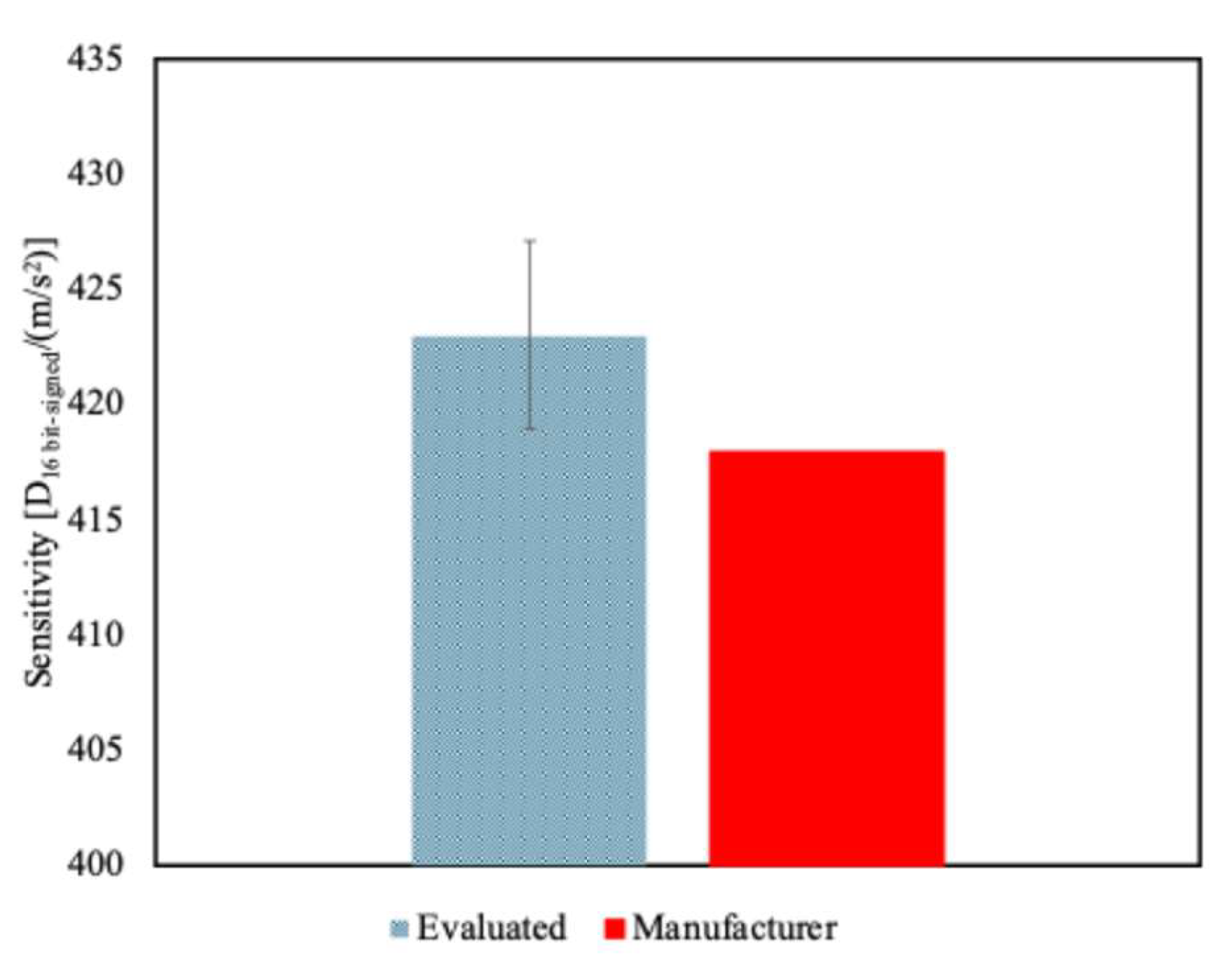

Table 1.
Description of the model parameters.
| Parameter | Description |
|---|---|
| α | Angle of inclination of the axis of rotation with respect to the vertical |
| β | Rotation angle of the accelerometer on the plane of the disk around its axis |
| Δs | Tangential displacement of the accelerometer |
| r | Distance of the sensitive element from the rotation axis |
| at | Tangential acceleration at the sensitive element position |
| ar | Radial acceleration at the sensitive element position |
| ap | Acceleration perpendicular to the disc surface (gravity component) |
| δ | Initial angular position of the accelerometer |
| θ | Angular position assumed by the accelerometer during oscillations, from the initial angular position δ |
Table 2.
Standard uncertainty budget.
| Type of contribution | Symbol | Estimation |
|---|---|---|
| Repeatability | ur | 0.05% |
| Linearity | ul | 0.05% |
| Reference | uref | 0.3% |
| Calibration Uncertainty | uc | 0.3% |
Table 3.
Uncertainty estimates for the sensitivity calculated on the basis of groups of data.
| Case | Group of data | Overall uncertainty |
|---|---|---|
| 1 | Single axes, single accelerometer | X: 0.8% Y: 0.6% Z: 0.7% |
| 2 | Single accelerometer | 0.9% |
| 3 | All accelerometer | 1% |
Disclaimer/Publisher’s Note: The statements, opinions and data contained in all publications are solely those of the individual author(s) and contributor(s) and not of MDPI and/or the editor(s). MDPI and/or the editor(s) disclaim responsibility for any injury to people or property resulting from any ideas, methods, instructions or products referred to in the content. |
© 2025 by the authors. Licensee MDPI, Basel, Switzerland. This article is an open access article distributed under the terms and conditions of the Creative Commons Attribution (CC BY) license (http://creativecommons.org/licenses/by/4.0/).
Copyright: This open access article is published under a Creative Commons CC BY 4.0 license, which permit the free download, distribution, and reuse, provided that the author and preprint are cited in any reuse.


