
Submitted:
29 October 2024
Posted:
29 October 2024
You are already at the latest version
Abstract
This paper presents an effective Levenberg-Marquardt procedure for modeling accelerometers used in the energy industry. The proposed procedure applies the results of accelerometer calibration methods commonly used in engineering practice using stationary or portable calibrators. These methods are extended here to more advanced solutions, which will constitute the basis for further research (both practical and theoretical) into improving the accuracy of accelerometers, which play an extremely important diagnostic function in the operation of machines, devices and the wide range of components used in the energy industry.
Keywords:
Levenberg-Marquardt procedure
; accelerometer
; accelerometer modelling
; energy industry
1. Introduction
Accelerometers have very important functions in applications in the energy industry, especially in the field of monitoring and diagnostics of the operation of machines and devices [1,2]. They play an important role in the early detection of damage by monitoring the operation of bearings in generators, engines, turbines, and various types of pumps and compressors [3]. Such sensors play a particularly important role in wind power plants, where they are used to monitor rotor vibrations caused by damage, balancing errors or the influence of atmospheric factors [4,5]. They are also very important components of hydroelectric power plants, as they detect vibrations of rotors or other moving elements [6]. Nuclear power plants are used for early detection of earthquakes or seismic effects, which negatively affect the operation of this type of power plant [7]. In addition, they are used to monitor transmission infrastructure to ensure the stability of high-voltage lines and supporting structures [8,9], and are indispensable diagnostic elements designed to detect leaks in oil or gas pipelines by monitoring changes in pressure or flow dynamics [10,11].
Due to the wide range of very important applications of accelerometers in the energy industry, systematic control systems are necessary, as their improper operation would disrupt the correct diagnostics and monitoring of the energy infrastructure [12]. Accelerometer control is carried out by means of calibration, which is carried out using specialised stationary calibrators or portable calibrators, which are becoming increasingly popular. This calibration is carried out by determining two basic characteristics [13,14]:
- – Linearity, which represents the dependence of the response signal amplitude on the excitation signal at a constant excitation frequency;
- – Amplitude-frequency response, which represents the relationship between the output signal amplitude to the input signal amplitude ratio and the changes in frequency over the range covering the accelerometer's operating frequency band.
However, in addition to the abovementioned calibration methods, which are traditionally applied in engineering practice, a very important role is also played by the elimination of dynamic error during the operation of the accelerometer at the diagnostic station [15]. The dynamic error is then the result of stimulating the accelerometer with dynamically changing undetermined signals, i.e. signals that are not repeatable as a function of time [16,17,18]. The dynamic error is typically eliminated using deconvolution filters, which perform inverse transformations [19]. However, such a transformation is only possible when the parameters of the mathematical model of the accelerometer (usually a second-order differential equation) are determined by modelling. This can be performed by determining the amplitude-frequency response of the corresponding accelerometer, but with the need to regulate the frequency over a range that exceeds the resonance state [20].
This paper presents a method of modelling accelerometers based on an iterative Levenberg-Marquardt procedure, which is used for regression of the amplitude-frequency response measurement points according to the least squares principle [21,22]. This procedure combines the Gauss-Newton and steepest descent methods and is therefore extremely effective for nonlinear regression tasks such as determining the amplitude-frequency response. The solutions presented in this paper are based on the measurement points of this response and are obtained by using the same calibrator as applied in the classical calibration of accelerometers.
Section 2 introduces some theoretical background to accelerometer modelling using second-order differential equations, derives mathematical formulas related to the amplitude-frequency response, and presents a detailed discussion of applying the Levenberg-Marquardt procedure to accelerometer modelling. Chapter 3 gives the calibration and modelling results of two selected accelerometers types. An example of the use of the deconvolution algorithm to eliminate the dynamic error of an accelerometer is also presented.
The solutions presented here constitute a new approach to accuracy tests of accelerometers in energy applications and can be successfully used in engineering practice, as a supplement to commonly applied calibration methods based on this type of sensor, and in theoretical studies of the optimisation of mathematical models of accelerometers, elimination of the dynamic error, and determination of the upper limit of the dynamic error, among others [20]. These solutions can significantly improve the diagnostic measurements performed by accelerometers in energy applications.
2. Materials and Methods
The mathematical model of the accelerometer is described by a second-order differential equation, as follows:
where and denote the static amplification factor, pulsation of natural undamped vibrations and damping factor, respectively.
The Laplace transform of the above equation with zero initial conditions gives
where denotes a Laplace operator, and is the imaginary number.
A simple transformation of Eq. (2) gives the formula
which represents the transfer function for the accelerometer [23].
When` Eq. (3) is considered as the accelerometer frequency response, we have
where and represent the amplitude-frequency and phase-frequency responses of the accelerometer. The following equations represent these responses:
and
where [rad/s], and [Hz] is the frequency [23].
In the following, we present graphical dependencies and mathematical relations that constitute the basis for modelling the accelerometer based on the amplitude-frequency response.
Figure 1 shows an exemplary amplitude-frequency response as a function of frequency, where and denote the resonance frequency and resonance peak, respectively. These parameters are typical variables for accelerometer modelling based on the amplitude-frequency response.
The resonant frequency is obtained by equating the following derivative to zero:
Simplification of Eq. (7) gives
and as a result,
The ordinate value corresponds to defines the resonance peak
For the frequency to be a real number, the following conditions must be met:
and hence
Solving Eq. (10) gives
Substituting Eq. (13) into Eq. (9) gives
By substituting Eqs. (13) and (14) into Eq. (5), as a function of the frequency , we obtain
which enables modelling of the accelerometer based on its amplitude-frequency response and using the Levenberg-Marquardt procedure.
The Levenberg-Marquardt procedure is an iterative method that allows us to determine the vector of unknown parameters using the following formula
where
and and are the Jacobian matrix of the dimension , the unit matrix with dimensions , the vector of the searched parameters of the accelerometer model, a scalar with a value that changes over successive iterations, and the error, while and denotes the total number of iterations. The parameter denotes the time quantisation step, where while the error determines the regression rate of the measurement points of the amplitude-frequency response obtained using the equation given by Eq. (15) and the least squares method [22].
The Levenberg-Marquardt procedure is carried out in two main steps:
Step 1 (:
1. Select the initial values of the vector
2. Set the initial value of the parameter (e.g. ).
3. Check the error
4. Calculate Eq. (17) and then Eq. (16).
5. Determine the values of vector
Step 2 (:
1. Update the values of the vector
2. Calculate Eq. (17) and then Eq. (16) and determine the values of vector .
3. Calculate the error
4. Compare the value of error for steps and If the error for step is is higher or equal than for step then multiply the parameter by the assumed value (e.g ) and return to point 2. If the error for step is lower than for step then divide the parameter by the parameter and then return to point 1. If the value of the error does not increase over the two consecutive stages within the accepted tolerance, then the stop condition is triggered.
3. Results and Discussion
This section presents a method of generating the measurement points of the amplitude-frequency response given by Eqs. (5) and (15) using the 9110D series portable calibrator [24].
Figure 2 shows the front panel of the portable calibrator, which enables accurate calibration of a wide range of accelerometers. This calibrator carries out 'back-to-back' calibration, in which the tested accelerometer is mounted directly on a reference accelerometer of a higher class than the one being tested. In this case, the reference accelerometer is a quartz ICP type sensor. The generated frequency range is 5–10 kHz, with a maximum load of 100 g. The maximum amplitude for a signal with a frequency of 100 Hz realised for the case of a calibrator without a load is 20 g/pk, which corresponds to a value of 196 The maximum load of the calibrator is 800 g. This calibrator is equipped with an intuitive user interface and display, which makes it easy to configure and monitor the calibration process. It also calculates and displays the sensitivity of the test sensor on the screen in real time, and has a built-in ICP input for calibrating typical piezoelectric sensors [24].
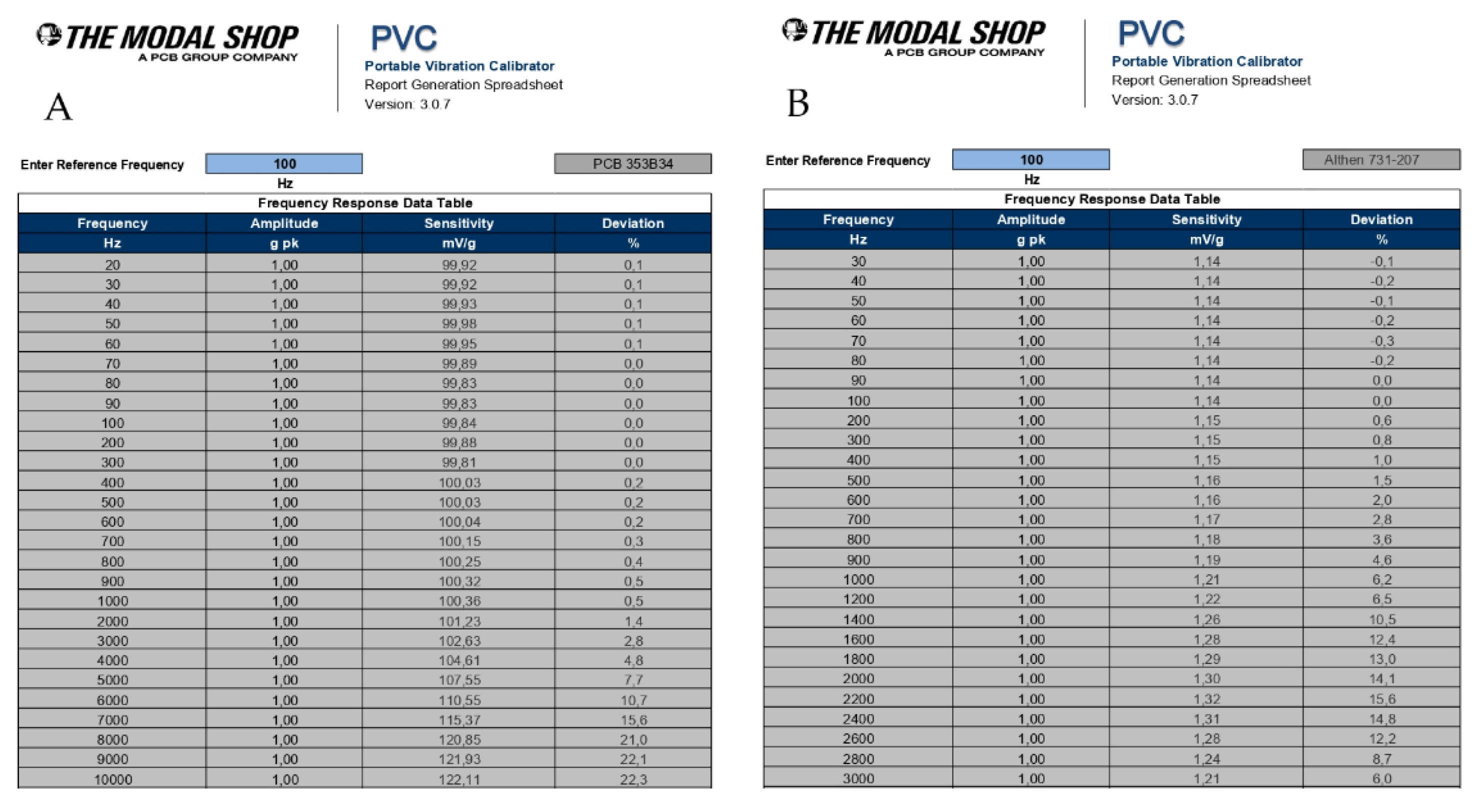
After calibrating the tested accelerometer over the selected frequency range, a table of measurement points is generated using dedicated software installed on a portable computer. This table contains four columns, which represent the frequencies [Hz], excitation amplitudes [g/pk], sensitivities [V/g] and deviations [%]. The measurement data are transferred via a USB drive from the calibrator's memory to the computer, and are loaded into the software used to generate the calibration certificate.
Table 1 shows the measurement data obtained for the two tested accelerometers. Panels A and B contain the data for the PCB 353B34 and Althen 731–207 accelerometers, which were tested for frequencies in the ranges 20–10,000 Hz and 30–3,000 Hz, respectively. For both accelerometers, the sensitivity and deviation values were determined for the 27 frequency values of the input excitation signal at a constant amplitude of 1 g/pk.
The PCB 353B34 accelerometer was tested with a step of 10 Hz up to a frequency of 100 Hz, and then with a 100 Hz step up to a frequency of 1 kHz, and finally with a 1 kHz step up to a frequency of 10 kHz. The Althen 731–207 accelerometer was tested up to a frequency of 1 kHz with the same steps as for the PCB 353B34 accelerometer, while in the frequency range above 1 kHz, the step was 200 Hz.
Next, the measurement data given in Table 1 were transformed using the same software into graphical form, representing the calibration certificates and the amplitude-frequency responses. Both responses are presented on a logarithmic scale here due to the wide range of frequencies considered for the input excitation signal. Figure 3 shows the calibration cerificates obtained for the PCB 353B34 (left) and Althen 731–207 (right) accelerometers.
The 5% deviations of the amplitude-frequency responses given in the corresponding datasheets for the PCB 353B34 and Althen 731–207 accelerometers are equal to 4 kHz and 650 Hz, respectively [25,26]. The certificate calibrations in Figure 3 confirm that for PCB 353B34, the 5% deviation of the above response exactly corresponds to the value declared in the datasheet, while for the Althen 731–207 accelerometer, the 5% deviation is equal to 900 Hz. This means that both accelerometers are functional and can be approved for further use.
In order to determine the parameters of the model given in Eq. (3) for both accelerometers, the Levenberg-Marquardt procedure was used in accordance with Eqs. (16) and (17) based on the measured data presented in Table 1. Figure 4 shows the regression results for the amplitude-frequency responses for the PCB 353B34 and Althen 731–207 accelerometers. This regression is presented on a logarithmic scale, in the same way as the calibration certificates in Figure 3.
When implementing the Levenberg-Marquardt procedure, the following assumptions were made:
- −
- The initial values of the parameters and were set to 100 mV/g, 9 kHz, 123 mV/g and 1.14 mV/g, 2.2 kHz, 1.33 mV/g for the PCB 353B34 and Althen 731–207 accelerometers, respectively;
- −
- The initial value of the parameter was set to ;
- −
- The value of parameter was set to two.
Transforming the amplitude-frequency response into a function of the parameters and rather than the parameters and makes the Levenberg-Marquardt procedure both easy to initialise and, more importantly, effective. This is due to the ease of estimating the initial values of the parameters and based on the measurement points of the amplitude-frequency response.
We denote the parameters of the models obtained for the accelerometers as and . The values of these parameters are 99.8 mV/g, 9898 Hz, 122.6 mV/g and 1.14 mV/g, 2.2 kHz, 1.32 mV/g for the PCB 353B34 and Althen 731–207 accelerometers, respectively.
We denote as the relationship between the error, which is given by the following equation:
where and denotes the number of measurement points of the amplitude-frequency response . is the function given in Eq. (15) and calculated for the parameters and
Figure 5 shows the relationship between the error given by Eq. (18) and the frequency , for the PCB 353B34 and Althen 731–207 accelerometers.
From Figure 5, it can be seen that the highest regression inaccuracy of the amplitude-frequency response occurs for values of the frequency of 8 kHz for the PCB 353B34 accelerometer and 3 kHz for the Althen 731–207.
The mean square error (MSE), which represents the accuracy of the regression of measurement points, was determined based on the following relation:
where denote the measurement data.
The values obtained for the MSE were equal to 0.241 and 53.9 for the PCB 353B34 and Althen 731–207 accelerometers, respectively. We recalculated the parameter values and for both accelerometers based on the parameter values and using Eqs. (13) and (14), and obtained = 12.98 kHz and = 0.457 for the PCB 353B34 and = 3.12 kHz and = 0.502 for the Althen 731–207.
The results of accelerometer modelling obtained by applying the Levenberg-Marquardt procedure offer a basis for the implementation of deconvolution methods aimed at eliminating the dynamic error. By representing Eq. (3) in the form of the equations of state, we have:
The algorithm for deconvolution of the input signal in digital form, after quantisation of the accelerometer output signal to its digital equivalent , has the following form [27]:
where
The estimate is obtained based on the parameter with steps equal to and , while the auxiliary parameters are obtained with a step equal to The initial value of the parameter is assumed to be equal to zero.
The matrix is calculated using the following equation:
where
and
is the identity matrix, while and are the base of the natural logarithm and the step for quantisation of the time , which corresponds to the accelerometer testing time.
Figure 6 shows the results of applying the deconvolution algorithm given in Eqs. (21) and (22).
The results of implementing the deconvolution algorithm presented in Figure 6 show that by modelling the accelerometer using the Levenberg-Marquardt procedure, it is possible to easily and effectively eliminate the dynamic error resulting from the non-ideal amplitude-frequency response for the frequency range of an accelerometer, i.e. one that does not have a constant value of the amplification factor for this range. The deconvolution algorithm allows for reconstruction of the shape of the signal at the accelerometer input based on the signal recorded at its output.
6. Conclusions
This paper describes the application of the Levenberg-Marquardt procedure for modelling accelerometers intended for applications in the energy industry. An example illustrating the modelling of two selected accelerometers, PCB 353B34 and Althen 731–207, has been presented. The research results obtained here indicate the high effectiveness of the proposed procedure and demonstrate that it offers an alternative to the Monte Carlo method, which requires the use of pseudo-random generators and has a major disadvantage in terms of significant computational time. This is due to the fact that in the proposed solution, the parameters of the accelerometer model, which are the initial parameters for the Levenberg-Marquardt procedure, are determined with considerable accuracy based on the measurement points of the amplitude-frequency response.
As a result of applying the Monte Carlo method, the values obtained for the parameters and were 2% lower, 5% higher and 1% lower for the PCB 353B34 accelerometer, respectively. For the Althen 731–207 accelerometer, the values of these parameters were 3% lower, 4% lower and 2% higher, respectively. These differences are due to the random nature of the Monte Carlo method and to the iterative way of performing calculations in the Levenberg-Marquardt procedure.
The solutions presented in this paper are based on the results of accelerometer calibration obtained using practical experiments, and may constitute a basis for further theoretical research in the field of optimisation of mathematical models of accelerometers and for practical research on eliminating the influence of dynamic error in order to increase the accuracy of this type of sensor.
Author Contributions
Conceptualisation, K.T.; methodology, K.T.; software, K.T.; validation, K.T., K.O., J.S. and J.K.; formal analysis, K.T, K.O., J.S. and J.K.; investigation, K.T; resources, K.T; data curation, K.T., K.O., J.S. and J.K.; writing – original draft preparation, K.T.; writing – review and editing, K.T.; visualisation, K.T.; supervision, K.T.; project administration, K.T.; funding acquisition, K.T.
Funding
This research was conducted at the Faculty of Electrical and Computer Engineering, Krakow University of Technology, and was financially supported by the Ministry of Science and Higher Education, Republic of Poland (grant no. E-1/2023).
Institutional Review Board Statement
Not applicable.
Informed Consent Statement
Not applicable.
Data Availability Statement
MDPI Research Data Policies.
Conflicts of Interest
The authors declare no conflict of interest.
References
- Ji, C. and Sun, W. Special Issue on Process Monitoring and Fault Diagnosis. Processes. 2024, 12, 1–4. [CrossRef]
- Ghazali, M.H.M and Rahiman, W. Vibration Analysis for Machine Monitoring and Diagnosis: A Systematic Review. Shock Vib. 2021, 1–25. [CrossRef]
- Wang, L. and Powrie, H. 9 – Advanced Techniques for Bearing Condition Monitoring. Electric Vehicle Tribology. 2024, 153–181. [CrossRef]
- Pryor, S.C. and Barthelmie, R.J. Wind Shadows Impact Planning of Large Offshore Wind Farms. Appl. Energy. 2024, 359, 1–12. [CrossRef]
- Beiter, P., Rand, J.T., Seel, J., Lantz, E., Gilman, P. and Wiser, R. Expert Perspectives on the Wind Plant of the Future. Wind Energy. 2022, 25/8, 1363–1378. [CrossRef]
- Nakai, M, Masumoto, T. and Asaeda, T. Strategic Siting of Hydroelectric Power Plants to Power Railway Operations with Renewable Energy. Sustainability. 2024, 16, 1–16. [CrossRef]
- Dawson, K. and Sabharwall, P. Light Water Reactor Nuclear Power Plant Commodity Cost Driver Analysis. Int. J. Nucl. Energy. 2020, 14/1, 34–49. [CrossRef]
- Nielsen, S., Østergaard, P.A. and Sperling, K. Renewable Energy Transition, Transmission System Impacts and Regional Development—A Mismatch between National Planning and Local Development. Energy. 2023, 278, 1–12. [CrossRef]
- Maroufmashat, A. and Fowler, M. Transition of Future Energy System Infrastructure; Through Power-to-Gas Pathways. Energies. 2017, 10, 1–22. [CrossRef]
- Peng, S., Zhang, Z., Ji, Y. and Shi, L. Optimization of Oil Pipeline Operations to Reduce Energy Consumption Using an Improved Squirrel Search Algorithm. Energies. 2022, 15, 1–19. [CrossRef]
- Stöhr, T., Reiter, V., Scheikl, S., Klopcic, N., Brandstätter, S. and Trattner, A. Hydrogen Quality in Used Natural Gas Pipelines: An Experimental Investigation of Contaminants According to ISO 14687:2019 Standard. Int. J. Hydrog. Energy. 2024, 67, 1136–1147. [CrossRef]
- Härtel, S., Gnam, J.P., Löffler, S. and Bös, K. Estimation of Energy Expenditure using Accelerometers and Activity-Based Energy Models—Validation of a New Device. Eur. Rev. Aging Phys. Act. 2011, 8, 109–114, ISSN: 1861-6909.
- Nez, A., Fradet, L., Laguillaumie, P., Monnet, T. and Lacouture, P. Comparison of Calibration Methods for Accelerometers used in Human Motion Analysis. Med. Eng. Phys. 2016, 38/11, 1289–1299. [CrossRef]
- Sinha, J.K. On Standardisation of Calibration Procedure for Accelerometer. Int. J. Hydrogen Energy. 286/1–2, 417–427. [CrossRef]
- Dichev, D., Diakov, D., Zhelezarov, I., Valkov, S., Ormanova, M., Dicheva, R. and Kupriyanov, O. A Method for Correction of Dynamic Errors When Measuring Flat Surfaces. Sensors. 2024, 24/16, 1–20. [CrossRef]
- Tomczyk, K. and Layer, E. Energy Density for Signals Maximising the Integral-Square Error. Measurement. 2016, 90, 224–232. [CrossRef]
- Dichev, D., Koev, H., Bakalova, T. and Louda, P. A Model of the Dynamic Error as a Measurement Result of Instruments Defining the Parameters of Moving Objects. Meas. Sci. Rev. 2014, 14, 183–189. [CrossRef]
- Dudzik, M., Tomczyk, K. and Jagiełło, A.S. Analysis of the Error Generated by the Voltage Output Accelerometer Using the Optimal Structure of an Artificial Neural Network. 19th International Conference on Research and Education in Mechatronics. June 2018, 7–11. [CrossRef]
- Tolooshams, B., Mulleti, S., Ba, D. and Eldar, Y. Learning Filter-Based Compressed Blind-Deconvolution. IEEE Trans. Signal Process. 2022, 1–12. [CrossRef]
- Tomczyk, K. Procedure Proposal for Establishing the Class of Dynamic Accuracy for Measurement Sensors using Simulation Signals with One Constraint. Measurement. 2021, 178, 1–8. [CrossRef]
- Boos, E., Gonçalves, D.S. and Bazán, F.S. Levenberg-Marquardt Method with Singular Scaling and Applications. Appl. Math. Comput. 2024, 474. [CrossRef]
- Tomczyk, K. Levenberg-Marquardt Algorithm for Optimization of Mathematical Models according to Minimax Objective Function of Measurement Systems. Metrol. Meas. Syst. 2009, 16/4, 599–606, ISSN 0860-8229.
- Tomczyk, K. and Layer, E. Accelerometer Errors in the Measurement of Dynamic Signals. Measurement. 2015, 60, 292–298. [CrossRef]
- Datasheet for portable calibrator 9110D series: https://www.modalshop.com/docs/themodalshoplibraries/datasheets/9110d-portable-vibration-calibrator-datasheet-ds-0103.pdf?sfvrsn=202f7b45_7 (accessed: 3 October 2024).
- Datasheet for PCB 353B34 accelerometer: https://www.pcb.com/products?m=353b34 (accessed: 3 October 2024).
- Datasheet for Althen 731–207 accelerometer: https://www.althensensors.com/uploads/products/datasheets/731-207-low-frequency-seismic-vibration-sensors-en.pdf (accessed: 3 October 2024).
- Layer. E. and Tomczyk, K. Signal Transforms in Dynamic Measurements. Springer Verlag. 2015, ISBN-13: 9783319365343.
Figure 1.
Example of an amplitude-frequency response of an accelerometer.
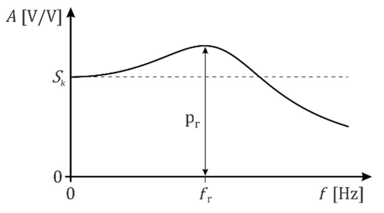
Figure 2.
Front panel of the series 9110D portable calibrator.
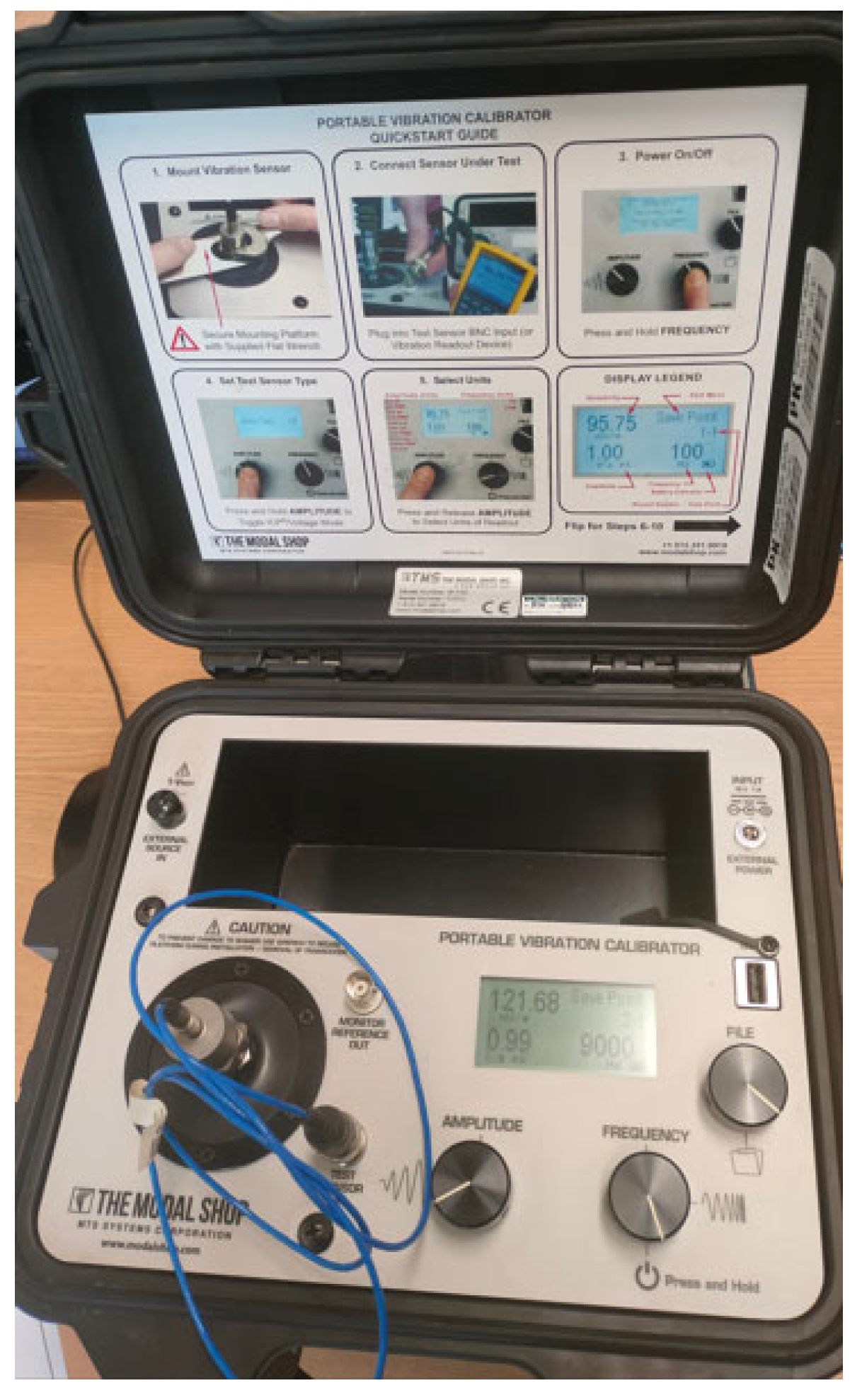
Figure 3.
Calibration certificates for the PCB 353B34 and Althen 731–207 accelerometers.
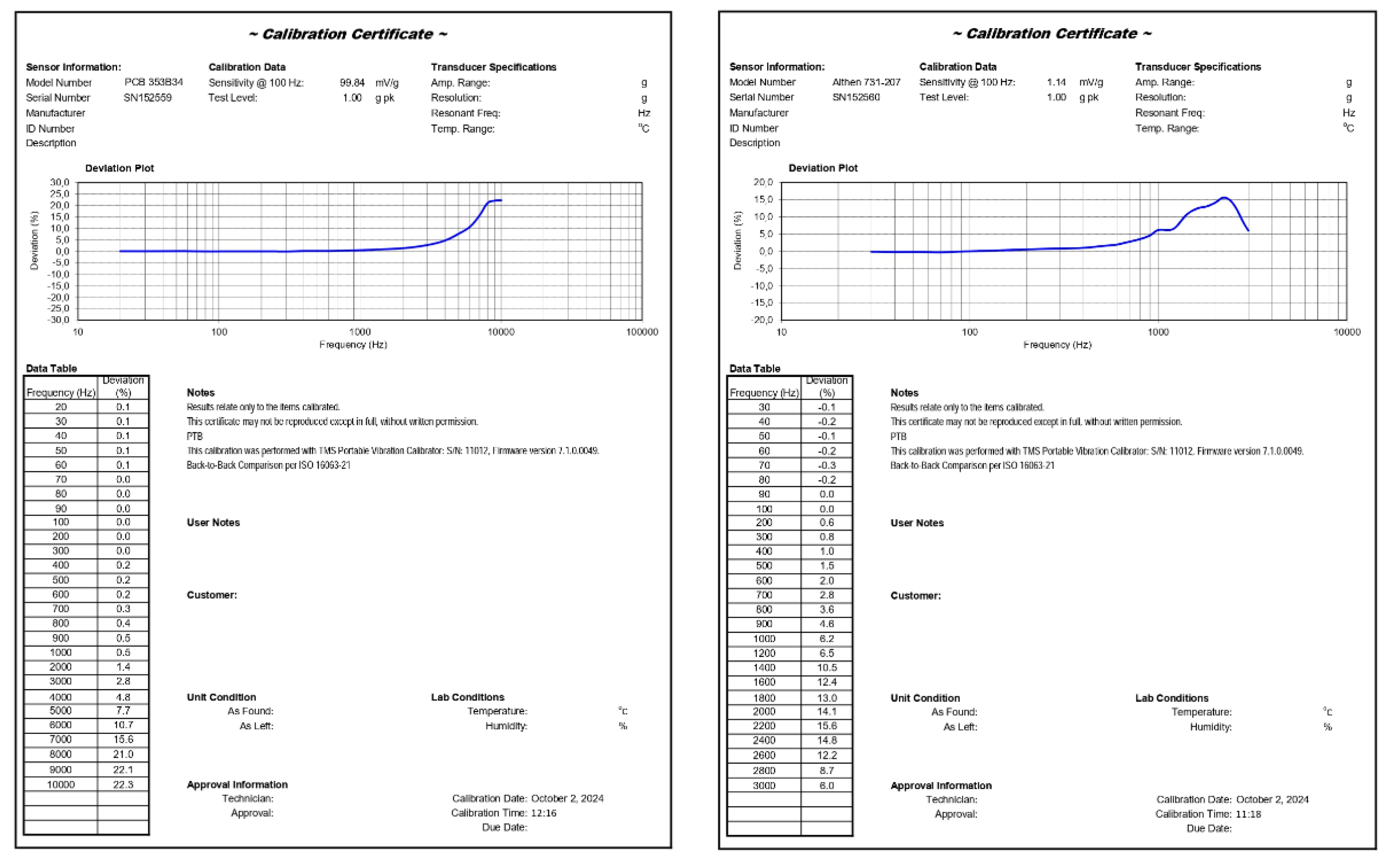
Figure 4.
Regression of the amplitude-frequency responses for the (a) PCB 353B34 and (b) Althen 731–207 accelerometers.
Figure 4.
Regression of the amplitude-frequency responses for the (a) PCB 353B34 and (b) Althen 731–207 accelerometers.
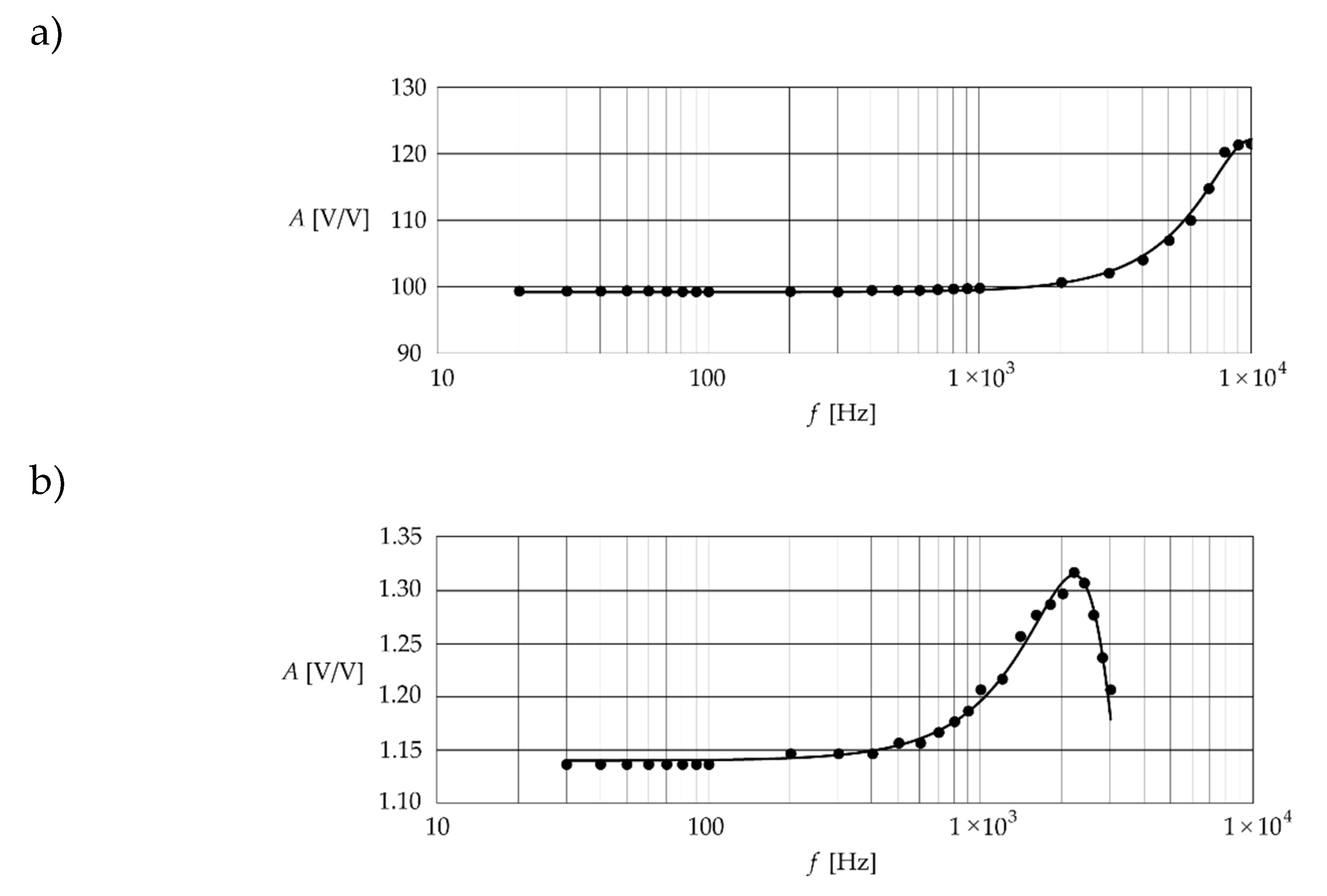
Figure 5.
Relationship between error and frequency for the (a) PCB 353B34 and (b) Althen 731–207 accelerometers.
Figure 5.
Relationship between error and frequency for the (a) PCB 353B34 and (b) Althen 731–207 accelerometers.
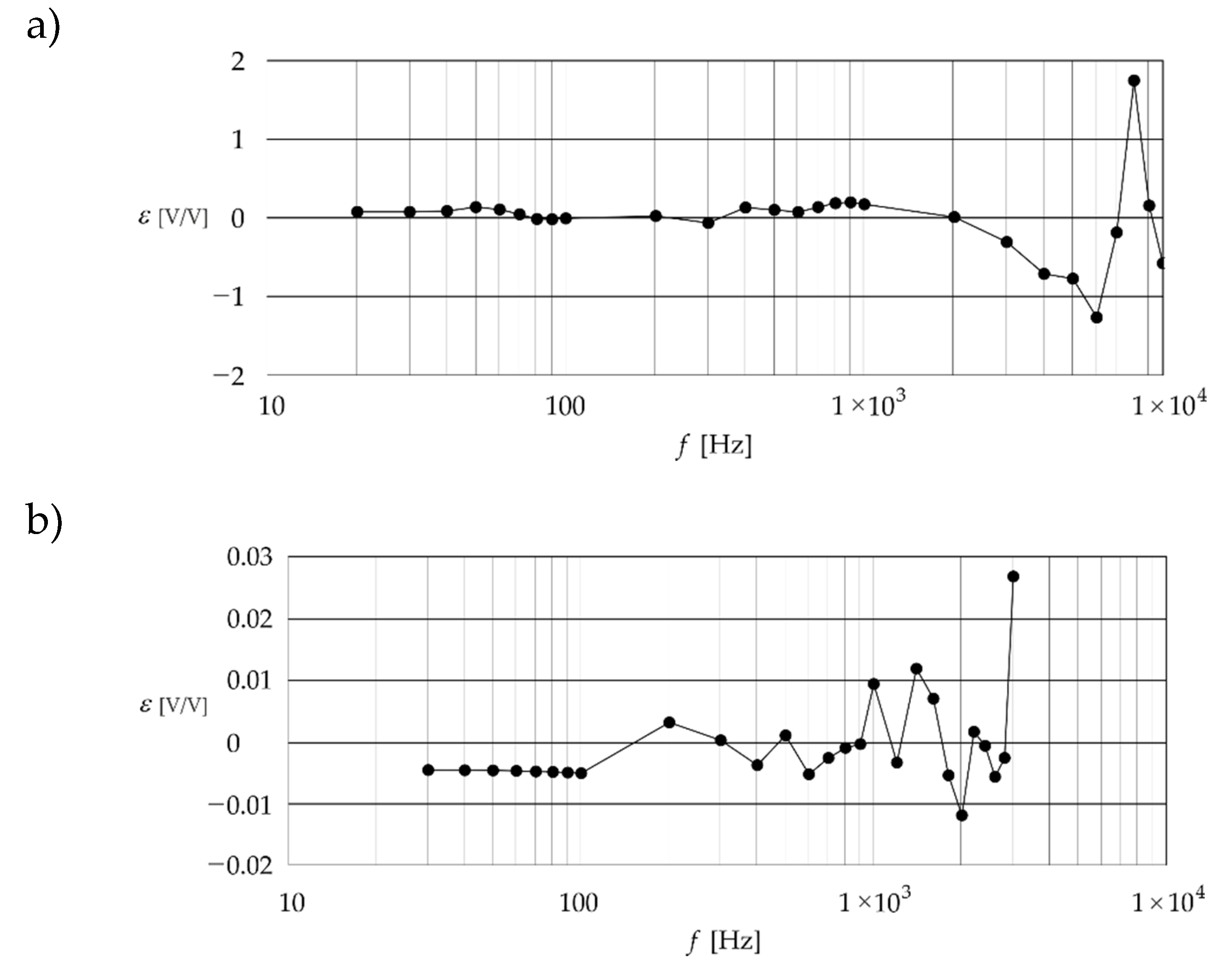
Figure 6.
Signal as a result of deconvolution of the output signal
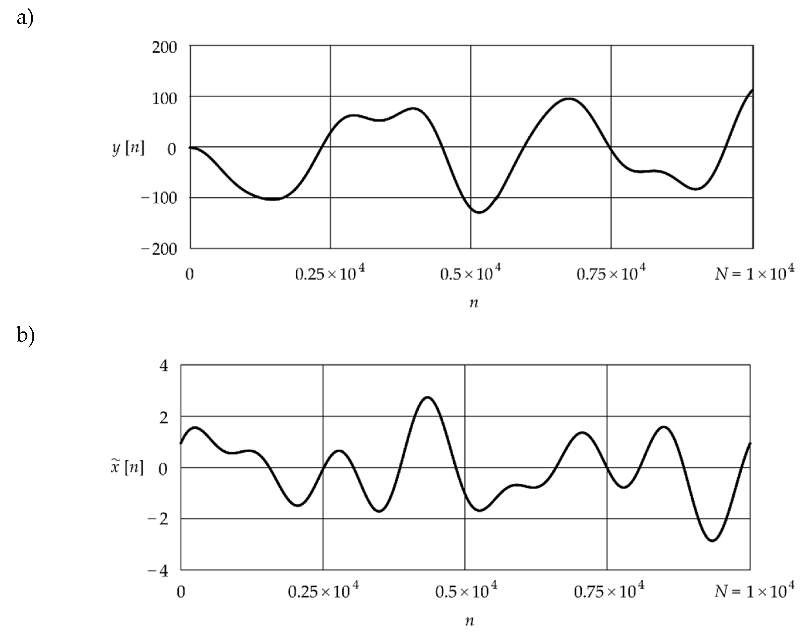

Table 1.
Measurement data for the PCB 353B34 (panel A) and Althen 731–207 (panelB) accelerometers.
Disclaimer/Publisher’s Note: The statements, opinions and data contained in all publications are solely those of the individual author(s) and contributor(s) and not of MDPI and/or the editor(s). MDPI and/or the editor(s) disclaim responsibility for any injury to people or property resulting from any ideas, methods, instructions or products referred to in the content. |
© 2024 by the authors. Licensee MDPI, Basel, Switzerland. This article is an open access article distributed under the terms and conditions of the Creative Commons Attribution (CC BY) license (http://creativecommons.org/licenses/by/4.0/).
Copyright: This open access article is published under a Creative Commons CC BY 4.0 license, which permit the free download, distribution, and reuse, provided that the author and preprint are cited in any reuse.


