
Submitted:
21 January 2025
Posted:
22 January 2025
You are already at the latest version
Abstract
The balanced flowmeter not only inherits the advantages of the orifice plate flowmeter but also stabilizes the flow field, reduces permanent pressure loss, and effectively increases the cavitation threshold. To deeply analyze flow characteristics through the perforated plate and achieve performance optimization for the liquid hydrogen (LH2) measurement, a numerical calculation framework based on the Mixture model, Realizable turbulence closure, and Schnerr-Sauer cavitation model is established. The model is first evaluated by comparing with the liquid nitrogen (LN2) experimental results of a self-developed balanced flowmeter as well as the measuring setup. The flow coefficient and pressure loss coefficient are especially concerned and the comparison with the orifice plane is made with the cavitation and non-cavitation conditions. The cavitation cloud and temperature contours are also present to illustrate the difference of measuring the upper limit of Re between water, LN2, and LH2 flow. The results show that compared to LN2 and water, LH2 has a larger cavitation threshold, indicating a wider range of Re number measurements.
Keywords:
Balanced flowmeter
; Perforated plate
; CFD
; Liquid hydrogen
1. Introduction
In the production, storage, transportation, and trade of cryogenic fluids such as liquid nitrogen (LN2) and liquid hydrogen (LH2), flow rate measurement is essential, which requires accurate, wide range, and reliable detection and maintenance. The orifice flowmeter realizes flow rate measurement according to the linear relationship between the pressure difference before and after the throttling orifice and the volume flow rate square. This kind of flowmeter has no moving parts, is simple, reliable, and low cost, and has been widely used. Compared with the traditional orifice flowmeter, the balanced flowmeter uses a perforated plate instead of a single orifice plate, which not only inherits the advantages of the latter but also can stabilize the flow field, reduce pressure loss, and delay cavitation occurrence, consequently, it shows a wider measuring range ratio and accuracy [1]. Therefore, it gradually replaces the latter to obtain more and more extensive applications.
Although the balanced flowmeter has been extensively studied with water as the working fluid [2,3,4]. For the application of the flowmeter to cryogenic fluids, the physical properties of cryogenic fluids differ greatly from that of water, as shown in Table 1 [5], and the temperature in the storage and transportation process of LN2 and LH2 is often close to the saturation temperature, so it is more prone to trigger cavitation [6]. The thermal effect of the cryogenic cavitation process cannot be ignored, thus, the LN2 and LH2 balanced flowmeter often presents more complex flow characteristics than that of water, requiring special optimization and calibration.
The application of a balanced flowmeter to cryogenic fluids is relatively late compared to the orifice type one. As early as 2006, Kelley et al. [7] invented a balanced plate for liquid oxygen measurement. They reported that compared with the orifice type, the upstream straight pipe length of the balanced one is required to be less than 0.5d, the pressure recovery rate is increased by 100%, the accuracy is improved by 10 times, and the noise intensity is reduced by 15 times [8]. In 2016, Liu et al. [9] studied the influence of fluid types on flow coefficient and static pressure loss coefficient through simulation. The results show that the lower limit of the Reynolds number of cryogenic fluids in the self-similar region is relatively close to that of water, but the cryogenic fluids have a higher upper limit of the Reynolds number. The pressure drop depends on the shape of the perforated plate and the physical properties of the fluid. Jin et al. [10] also carried out numerical research on the effects of hole distribution on measuring accuracy. They designed a plate with a central distribution of circular holes and pointed out that the plate with a slightly larger diameter central hole is more suitable for LH2 measurement than the plate with an equal hole diameter. In 2017, Shaaban et al. [11] designed a new balanced flowmeter with improved LH2 distribution by carrying out multi-dimensional and multi-objective optimization through numerical simulation. The results show that the flowmeter has improved flow coefficient, static pressure loss coefficient, and cavitation characteristics compared with the flowmeter designed by Jin et al. [10]. In 2018, Wang Jie [12] used LN2 as a working fluid to compare the performance of a balanced flowmeter under different inlet temperatures and outlet pressures by numerical method. The results show that a higher upper limit of Re number can be obtained in the self-similar region by reducing the inlet temperature or increasing the outlet pressure. While, for the experimental study of the cryogenic balanced flowmeter, few research results have been reported until now, except with the work by Tian [13] in 2016, who carried out an experimental study using LN2 as a working fluid.
To explore the flow characteristics of LH2 through the perforated plate in a balanced flowmeter, this paper established a numerical calculation framework based on the “single-phase flow” Mixture model, Realizable turbulence closure, and Schnerr- Sauer cavitation model. The thermal effect with cryogenic cavitation was considered. To evaluate the model, two balanced flowmeters and an LN2 flowrate experimental setup were designed and built to measure the flow coefficient and pressure loss coefficient. Then, based on the validated model, the flow process of the perforated plate under non-cavitation and cavitation conditions was investigated with water, LN2, and LH2 as the working fluids. The cavitation cloud, turbulence distribution, and temperature contours are present with the three fluids, and their effects on the measuring range are analyzed. The results can help to understand the mechanisms and characteristics of the LN2 and LH2 balanced flowmeter.
2. Numerical Model
Conservation Equations
When the pressure drops to the saturation value corresponding to the local temperature, cavitation will be triggered and the generated bubble cloud will detach from the wall and flow downstream of the perforated plate with the mainstream fluid. Simultaneously, the temperature will drop inside the cavitation regime. Thus, it is necessary to establish a mathematical model considering cavitation with thermal effects in the simulation. The calculation for cavitating flow in a perforated plate adopts the homogeneous model. It simplifies the "two-phase fluid" to "single-phase one" and ignores the slip velocity between the two phases, which means that the two phases share the same velocity. The inlet Re numbers for the working conditions are in the range of 104~106, which is a compressible turbulent flow. Thus, the conservation equations of continuity, momentum, energy, and vapor mass transport of the mixture are as follows:
1) Mass conservation qutation
Here, uj is the velocity and ρm and is the vapor fraction weighted average density of the mixture, which is calculated as and the same below:
α is the phase fraction, and subscripts v and l are vapor and liquid phases, respectively.
2) Momentum equation
Here,p is pressure, is gravitational acceleration. μm and μt is the laminar and turbulent viscosity of the two-phase mixture, respectively.
3) Energy equation
Here, hm is the enthalpy of the mixture, λm, and λt is the laminar and turbulent thermal conductivity, respectively. T is temperature and SE is the volume heat source due to phase change:
SE=-ht·R
Here, ht is the latent heat of phase change, and R is the net mass transfer rate between the phases.
4) Vapor volume transport equation
Here, RE and RC are the mass sources due to evaporation and condensation, respectively.
In addition, the ideal gas equation is used to calculate the vapor density. The other physical properties of fluids in the simulation, such as density ρl, dynamic viscosity μ, specific heat capacity cp, thermal conductivity λm, and saturation pressure pv are all functions of temperature, obtained from REFPROP 8.0 [5].
5) Turbulent closure
Due to the Reynolds stress in the Realizable k-ε model being more in line with mathematical constraints, consistent with turbulence mechanisms, and providing better descriptions of streamline and vortex characteristics, the turbulent model has been widely used to simulate cryogenic cavitating flow. The equations for turbulent kinetic energy k and turbulent kinetic energy dissipation rate ε are as follows.
Where, ,,,Gk is the turbulent kinetic energy generated by the average velocity gradient, Gb is the turbulent energy generated by buoyancy, and YM is the total turbulent energy dissipation rate due to the compressible effect. The constant terms in the model are: σk=1.0, σε=1.2, Cμ=0.09, C1=max[0.43, η/(η+5)], C2=1.9, C1ε=1.44.
6) Cavitation model
The modeling of cryogenic cavitation needs to consider the thermodynamic effects. The Schnerr-Sauer model considers the thermodynamic effects and has proved that when the bubble number density is nb=108, the model can better predict the cavitating flow of cryogenic fluids [14]. The final form equation is [15]:
3. Model Validation
The modeled geometry consists of a perforated plate and the upstream and downstream pipelines with an inner diameter of D=50 mm. Due to the symmetrical structure of the plate, to ensure both high efficiency and accuracy of the simulation, the model is simplified to a quarter of the total. Figure 1 shows the three-dimensional structure and cross-sectional view of the computational domain. To ensure the full development flow upstream and complete recovery of static pressure downstream, the lengths of the straight pipes upstream and downstream of the plate are set to 10D and 15D, respectively.
The equivalent diameter ratio β=0.1-0.75 is recommended, β=De/D, De is the equivalent diameter of the total opening area of the perforated plate. Correspondingly, the single hole size and distribution of perforated plates are preliminarily designed, as shown in Figure 2, which consists of a central hole and a circle of uniformly distributed small holes around it. Among them, D1=D2=10 mm and Dr=30.86 mm are used to represent the diameter of the central hole, surrounding holes, and distributed circle, respectively. t= 3 mm is the plate thickness.
The sub-zone grid scheme is adopted, that is, the grid inside the holes and the surroundings is specially densified, while the grid of the pipelines upstream and downstream are sparsed to save computing resources, as shown in Figure 3.
The inlet and outlet of the pipeline are set as velocity inlet and pressure outlet boundary conditions respectively. During the calculations, through fixed outlet pressure and adjustable inlet velocity, different inlet Re numbers.
The coupling between pressure and velocity adopts the "Coupled" algorithm. The discretization of the pressure and vapor phase volume fraction terms respectively adopts the "PRESSO!" and "QUICK" algorithms; The discretization of momentum, energy, and turbulence terms all adopts the second-order upwind algorithm. The convergence satisfies the following criteria simultaneously: (1) the residual values of the continuity and momentum equation are less than 10-3, and that of other indicators is less than 10-6; (2) The error of inlet and outlet volume flowrate is less than 0.1%.
To verify grid independence, grid numbers 1007340, 1519930, 2032520, and 2545110 are checked for calculation. The main difference between them is the number of nodes inside the holes of the plate. LN2 was used as the working fluid with inlet velocities of 2.4m/s, 3.2m/s, 4.0m/s, 4.8m/s, and 5.6m/s, which includes non-cavitation and cavitation conditions. The flow coefficient C and static pressure loss coefficient ζ are obtained, as shown in Figure 4, where C is defined as the ratio of measured flow rate to theoretical value, and ζ =ΔP/(0.5ρu2), ΔP is the pressure difference between the tap. The changes in C and ζ for grid 2032520 and 2545110 are less than 0.3% and 0.5%, respectively. Therefore, to improve computational speed, the following calculations adopt a mesh scheme with a grid number of 2032520.
According to the geometric parameters in Figure 2 and concerning the international standard ISO 5167-2 [13], we designed and manufactured a DN50 balanced flowmeter, as shown in Figure 5. the parameters are listed in Lable 2.

Table 2.
Geometrical parameters for the test perforated plate.
| Type | Inner diameter D (mm) | β | Thickness t (mm) |
Number of surrounding holes N |
D1/D2 |
Dr (mm) |
| Orifice | 50 | 0.6 | 3 | 0 | \ | \ |
| Perforated | 8 | 1 | 32.26 |
Due to the scarcity of experimental data for LH2 balanced flowmeters, we constructed a DN50 LN2 experimental rig for flowrate measurement based on the standard flowmeter, as shown in Figure 6. The main components include: an injection Dewar with a volume of 300L and rated pressure of 0.6MPa, a standard LN2 flowmeter (Hoffer-hfc2000, Accuracy: ± 0.2% FS), a vacuum chamber with the test flowmeter inside, a cryogenic control valve, and a collection Dewar. The LN2 is pressurized out of the Dewar by the high-pressure nitrogen gas, and due to the vertical flow of LN2 from bottom to top, the single-phase state and measurement accuracy of the standard cryogenic flowmeter are ensured. The temperature is measured by a PT100 thermometer with an accuracy of ± 0.05k.
Figure 7 shows the numerical and experimental results of the flow coefficient C and static pressure loss coefficient ζ of the orifice and perforated plate with different Re. Compared with orifice plate. It is found that the average flow coefficient C of the perforated plate increased by 16.1%, and the average static pressure loss coefficient ζ decreased by 9.8%. Thus, the preferred porous plate can be better used for the measurement of LN2 flow. The quantitative deviation of numerical results compared to the experimental one is about 5%, which may be caused by the fact that the working conditions in the actual measurement are difficult to be completely consistent with those in the numerical simulation. Overall, the simulation results are consistent with the experimental results qualitatively, and the accuracy of the numerical model is verified.
4. Modeling and Analysis of LH2 Balanced Flowmeter
Taking the above developed perforated plate as the research object, water, LN2, and LH2 are selected and modeled for comparison with the inlet temperature is 300K, 77.36K, and 20.37K, respectively, and the out pressure is all set as 0.2MPa. The results are shown in Figure 8 and Figure 9. It can be seen that compared with water, the variation range of flow coefficient C and static pressure loss coefficient ζ of LN2 before the onset of cavitation is similar and smaller, the average C value decreases by 1.0%, the average ζ value increases by 1.9%, while, the upper limit of Re number ReU for LN2 fluid increases from 2.99 × 10⁵ to 10.65 × 10⁵. Compared with LN2, the variation of the C and ζ of LH2 under non-cavitating conditions are relatively consistent, the average C and ζ are relatively close, while the ReU increases show a significant improvement from 10.65 × 10⁵ to 37.82 × 10⁵. This means that the Re range of LH2 is greatly improved compared to LN2. In addition, when Re<10.65×10⁵, due to the almost identical C and ζ values of LH2 and LN2, the flowmeter can be directly used for the measurement of two fluids. The C value calibrated with LN2 has an error of 0.4% when directly used for LH2, which can be eliminated by correction.
Figure 10 shows the axial velocity and turbulence intensity contours of the three fluids under non-coitation conditions. It can be seen that compared with water, at the same inlet velocity, the velocity of LN2 and LH2 in the hole is slightly higher, the area of the vortex zone at the hole inlet and downstream of the perforated plate is slightly larger, and the turbulence intensity at the two places is also slightly higher. In addition, Figure 11 shows the cavitation and turbulence intensity contours of the three fluids under the cavitation condition. It indicates that the LN2 is more sensitive to cavitation than the other two fluids, and the turbulence intensity downstream of the perforated plate is also high. However, as the inlet velocity continues to increase, the pressure drop of all fluids through the plate, as well as the cavitation intensity, also continues to increase. Figure 12 shows the axial cavitation cloud and temperature contours of LH2, which show that the cavitation process of LN2 and LH2 is accompanied by a decrease in temperature. Therefore, compared with water, the LN2 and LH2 flow slightly increase the losses at the entrance of the hole and downstream of the perforated plate. In the non-cavitation condition, the flow field characteristics of LN2 and LH2 are relatively consistent, but in the cavitation condition, the onset of cavitation of LN2 occurs earlier. The cavitation vapor in the orifice reduces the effective flow area and, therefore, leads to higher static pressure loss.
5. Conclusions
The numerical study of a cryogenic balanced flowmeter with LN2 and LH2 as working fluid was carried out. The computational framework was based on the Mixture "single-phase flow" model, the Realizable turbulence model, and the Schnerr Sauer cavitation model. The model was verified by comparing it with the experimental data of the LN2 flow rate. Then, the flow field characteristics of the perforated plate under non-cavitation and cavitation conditions are simulated and compared between the results of water, LN2, and LH2. Also, the measurement performance of the orifice plate and perforated plate was compared. The following conclusions were obtained:
1. In non-cavitation conditions, the pressure drop coefficient hardly changes with Re; Under cavitation conditions, cavitation first occurs at the entrance of the hole, which leads to a decrease in the effective flow area of the liquid and an increase in static pressure loss. Compared with the orifice plate, the perforated plate significantly increases the Re upper limit of the non-cavitation zone, thus significantly expanding the measurement range.
2. Different working fluids affect measurement stability and Re upper limit of the balanced flowmeter. Compared with water, LN2 can obtain a relatively stable flow coefficient C, but cavitation occurs earlier and the measurement upper limit is lower compared to LH2. The lower density of LH2 results in a lower pressure drop and higher measurement limit.
Acknowledgments
This work is supported by the National Key Research and Development Program of China (No.2022YFB4002900) and the Natural Science Foundation of Zhejiang Province (BMHY25A020001).
References
- Malavasi, S.; Messa, G.V.; Fratino, U.; et al. On cavitation occurrence in perforated plates. Flow Measurement and Instrumentation 2015, 41, 129–139. [Google Scholar] [CrossRef]
- Zhao, T.; Zhang, J.; Ma, L. A general structural design methodology for multi-hole orifices and its experimental application. Journal of Mechanical Science and Technology 2011, 25, 2237–2246. [Google Scholar] [CrossRef]
- Mehmood, M.A.; Ibrahim, M.A.; Ullah, A.; et al. CFD study of pressure loss characteristics of multi-holed orifice plates using central composite design. Flow Measurement and Instrumentation 2019, 70, 101654. [Google Scholar] [CrossRef]
- You, K.; Lee, H.; Cho, J. Effects of Chamfered Perforated Plate on Pressure Loss Characteristics. Journal of the Korean Society for Aeronautical & Space Sciences 2019, 47, 779–786. [Google Scholar]
- Lemmon, E.W.; Huber, M.L.; McLinden, M.O. Reference fluid thermodynamic and transport properties–REFPROP Version 8.0. NIST standard reference database, 2007, 23.
- Wei, A.; Yu, L.; Qiu, L.; et al. Cavitation in cryogenic fluids: A critical research review. Physics of Fluids 2022, 34, 101303. [Google Scholar] [CrossRef]
- Kelley, A.R.; Van Buskirk, P.D. Balanced orifice plate: U.S. Patent 7,051,765[P]. 2006-5-30.
- Kelley A, R. Balanced Flow Metering and Conditioning: Technology for Fluid Systems[C]. Instrumentation Symposium for the Process Industries. 2006, 77842, 1–6. [Google Scholar]
- Liu, H.; Tian, H.; Chen, H.; et al. Numerical study on performance of perforated plate applied to cryogenic fluid flowmeter. Journal of Zhejiang University-Science A 2016, 3, 230–239. [Google Scholar] [CrossRef]
- Jin, T.; Tian, H.; Gao, X.; et al. Simulation and performance analysis of the perforated plate flowmeter for liquid hydrogen. International Journal of Hydrogen Energy 2017, 42, 3890–3898. [Google Scholar] [CrossRef]
- Shaaban, S. Design and optimization of a novel flowmeter for liquid hydrogen. International Journal of Hydrogen Energy 2017, 42, 14621–14632. [Google Scholar] [CrossRef]
- Wang Jie. Study on the influencing factors of flow characteristics of perforated plate in cryogenic balanced flowmeter[D]. Zhejiang University, 2018. [In Chinese].
- Tian Hong. Research on the characteristics of perforated plate flowmeters applied to cryogenic fluid[D]. Zhejiang University, 2016. [In Chinese].
- Zhu, J.; Chen, Y.; Zhao, D.; et al. Extension of the Schnerr–Sauer model for cryogenic cavitation. European Journal of Mechanics-B/Fluids 2015, 52, 1–10. [Google Scholar] [CrossRef]
- Schnerr, G.H.; Sauer, J. Physical and numerical modeling of unsteady cavitation dynamics[C] //Fourth international conference on multiphase flow. New Orleans, LO, USA: ICMF New Orleans, 2001, 1.
Figure 1.
Three-dimensional structure and cross-sectional view of the computational domain.
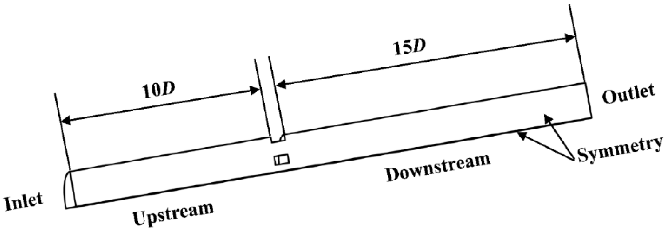
Figure 2.
Geometric parameters of perforated plate.
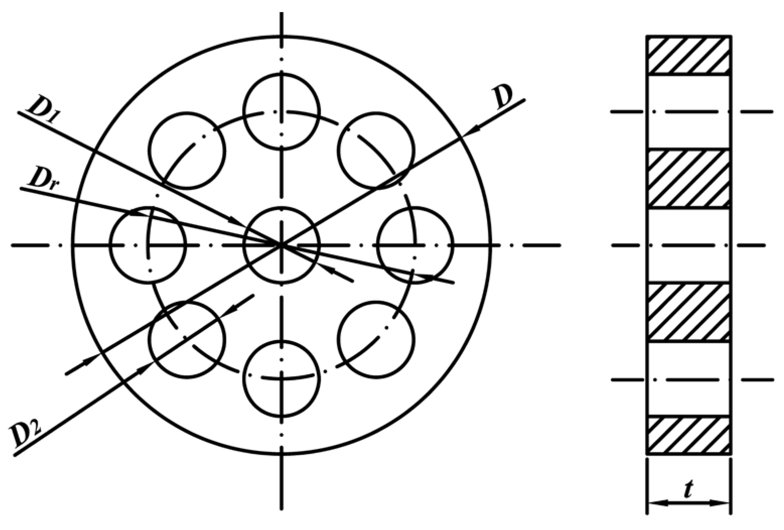
Figure 3.
Grid scheme for computational domain.
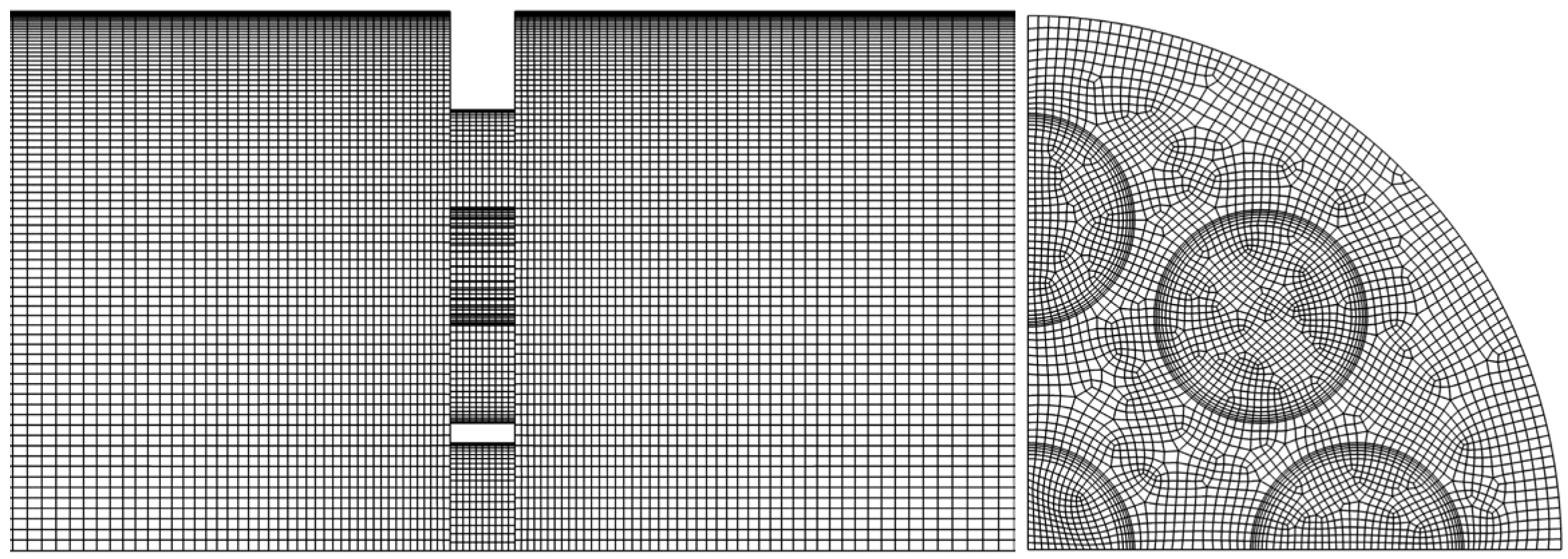
Figure 4.
Grid-independent verification.
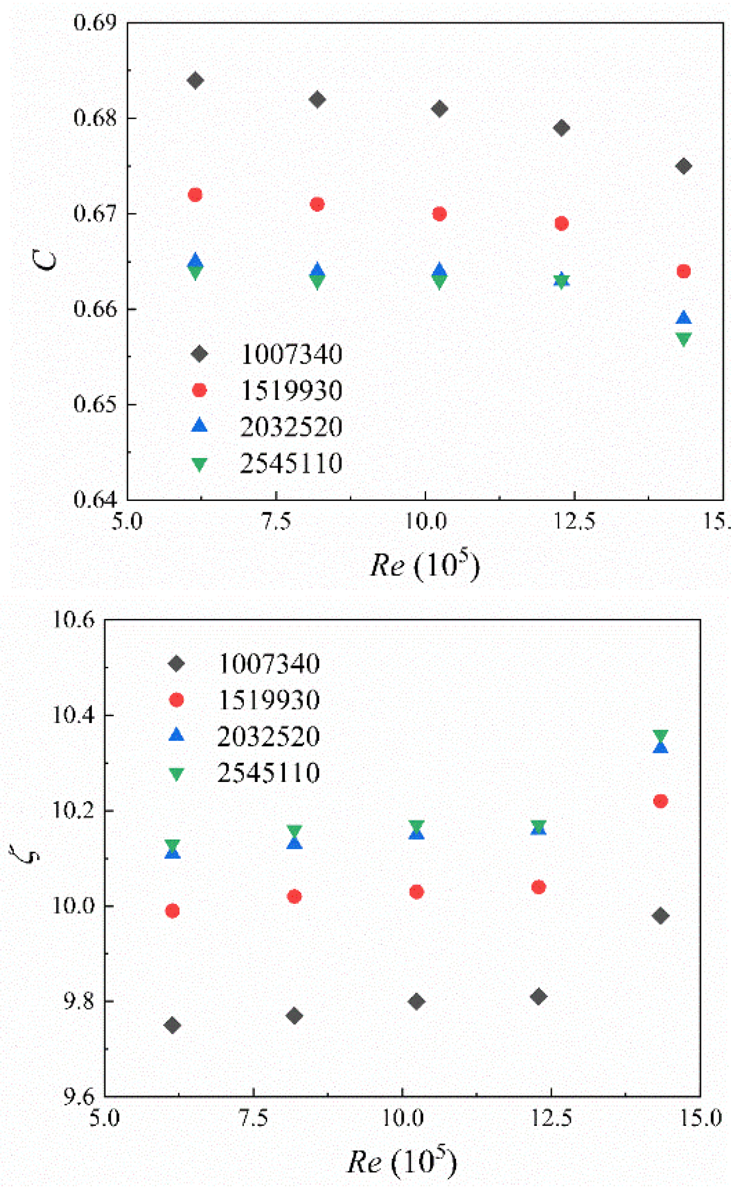
Figure 5.
Designed cryogenic balanced flowmeter.
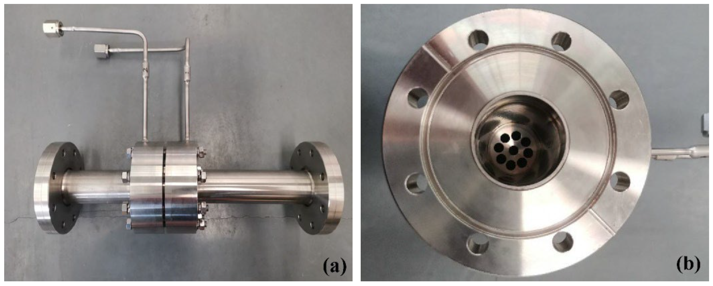
Figure 6.
LN2 flow rate experimental rig(Left) and schematic (Right).
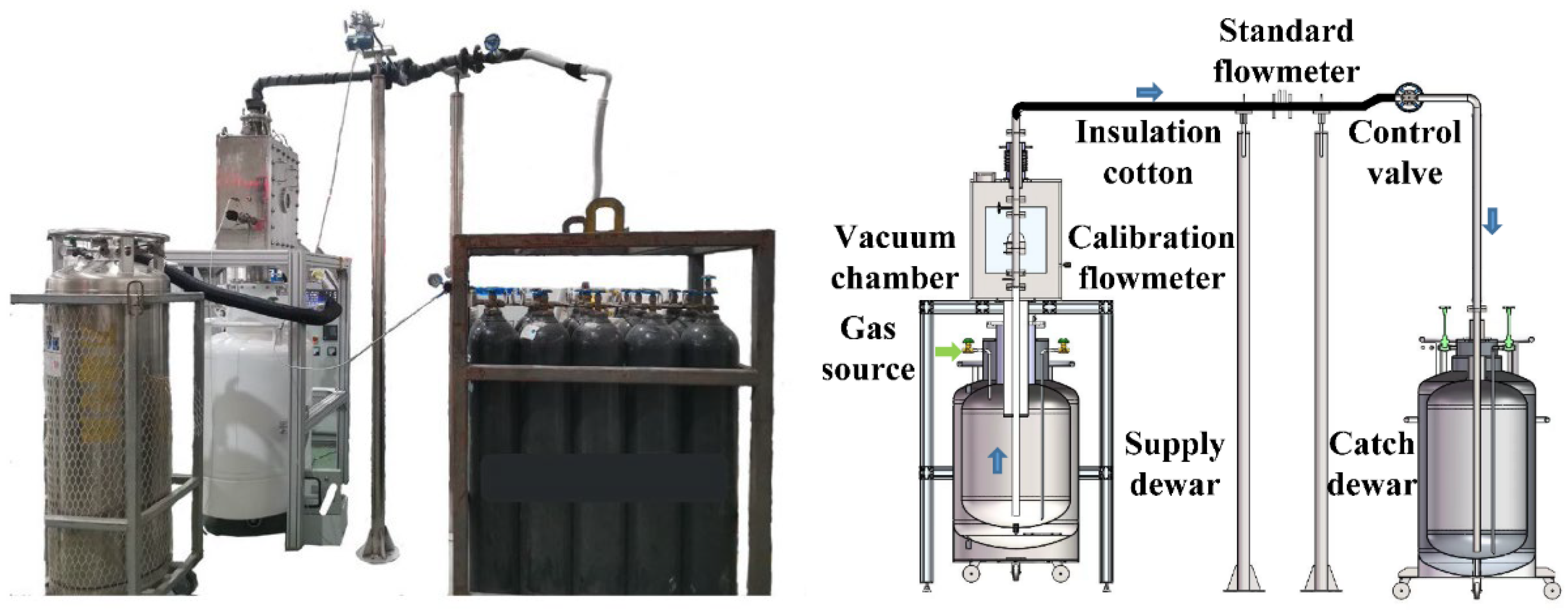
Figure 7.
Comparision of simulation with experiments for the orifice and perforated plane with LN2.
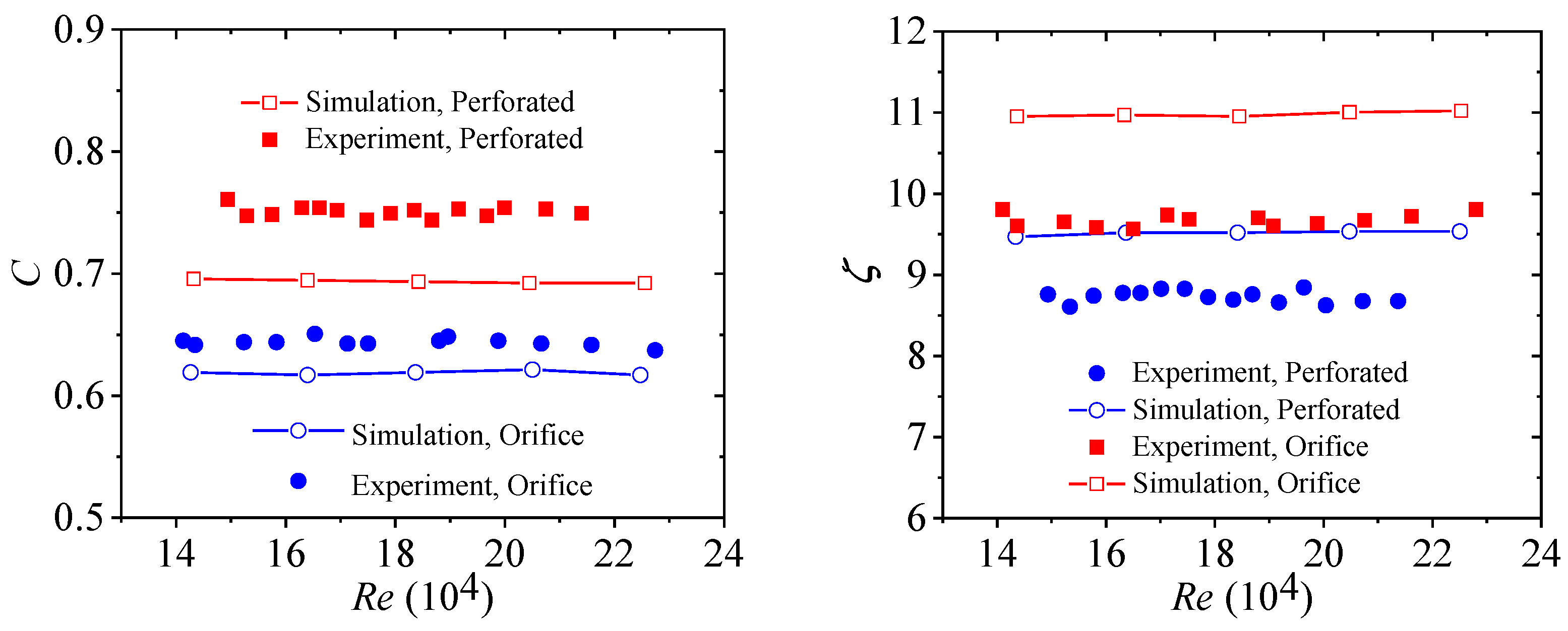
Figure 8.
Comparison of performance at different flow rates with water and LN2.
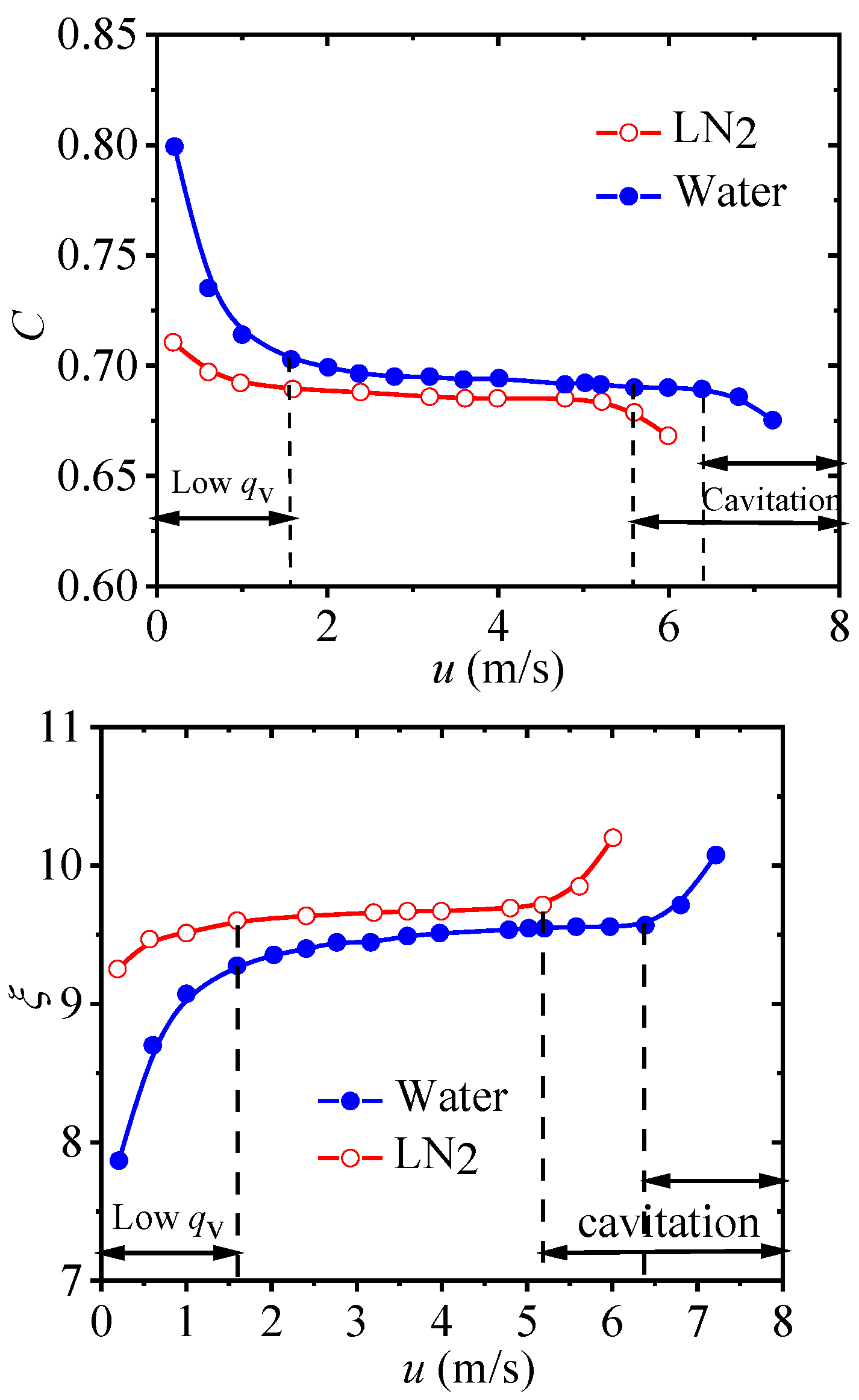
Figure 9.
Comparison of performance at different flow rates with LN2 and LH2.
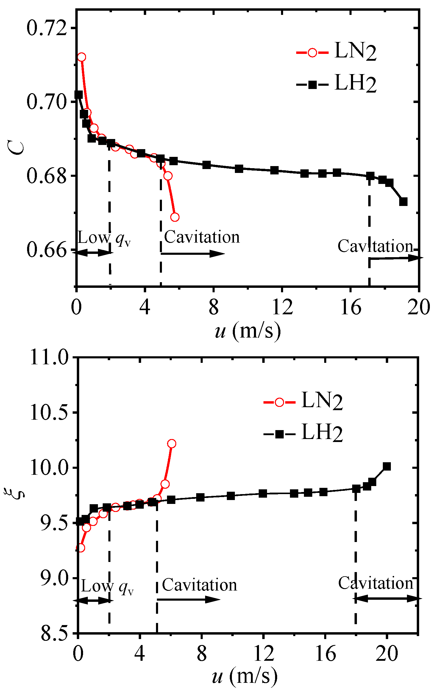
Figure 10.
Axial velocity and turbulence intensity contours of water, LN2, and LH2 (u=4m/s).
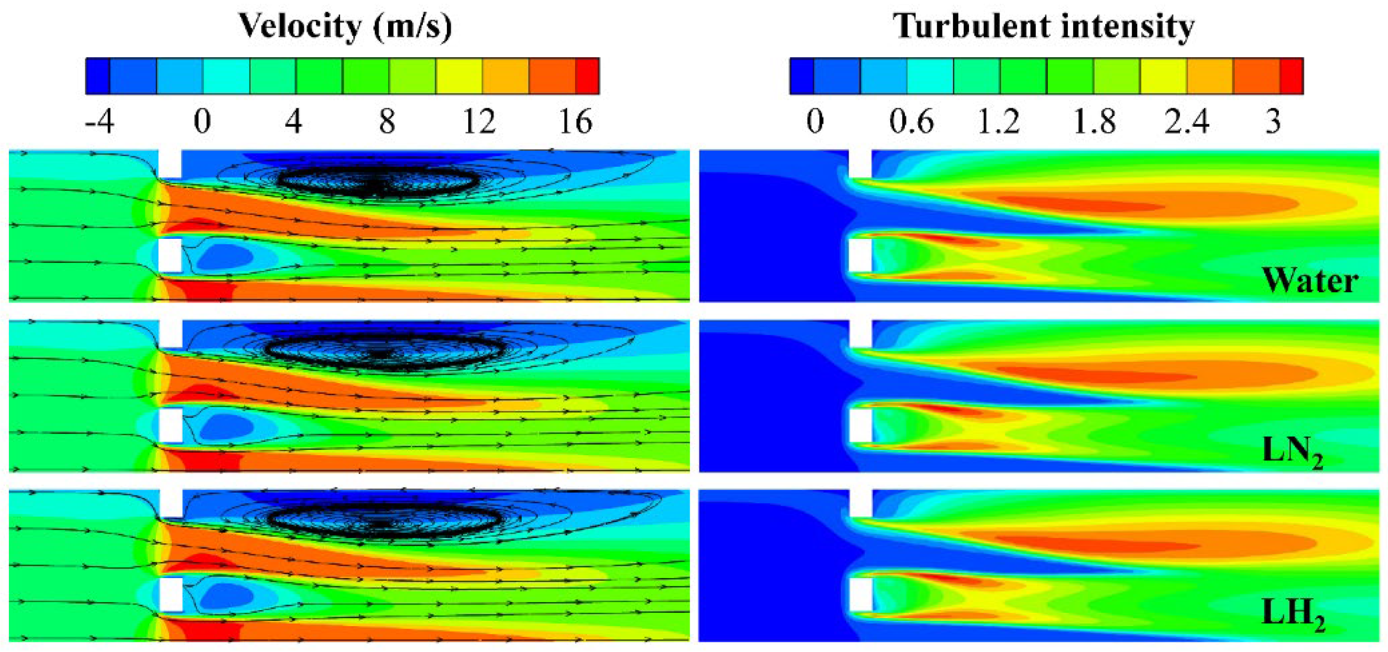
Figure 11.
Cavitation and turbulence intensity coutours of water, LN2 and LH2 (u=6 m/s).
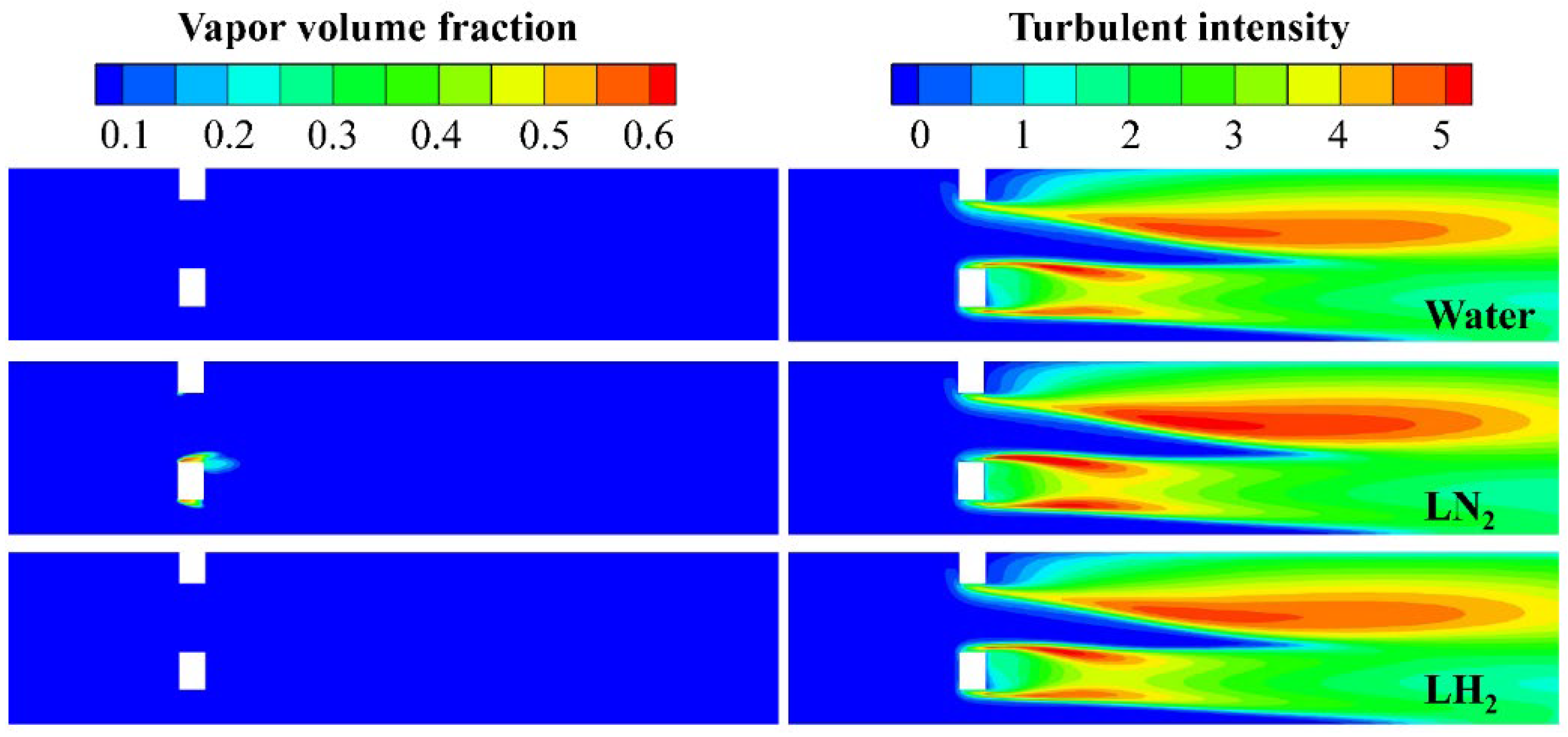
Figure 12.
Cavitation and temperature contours of LH2.
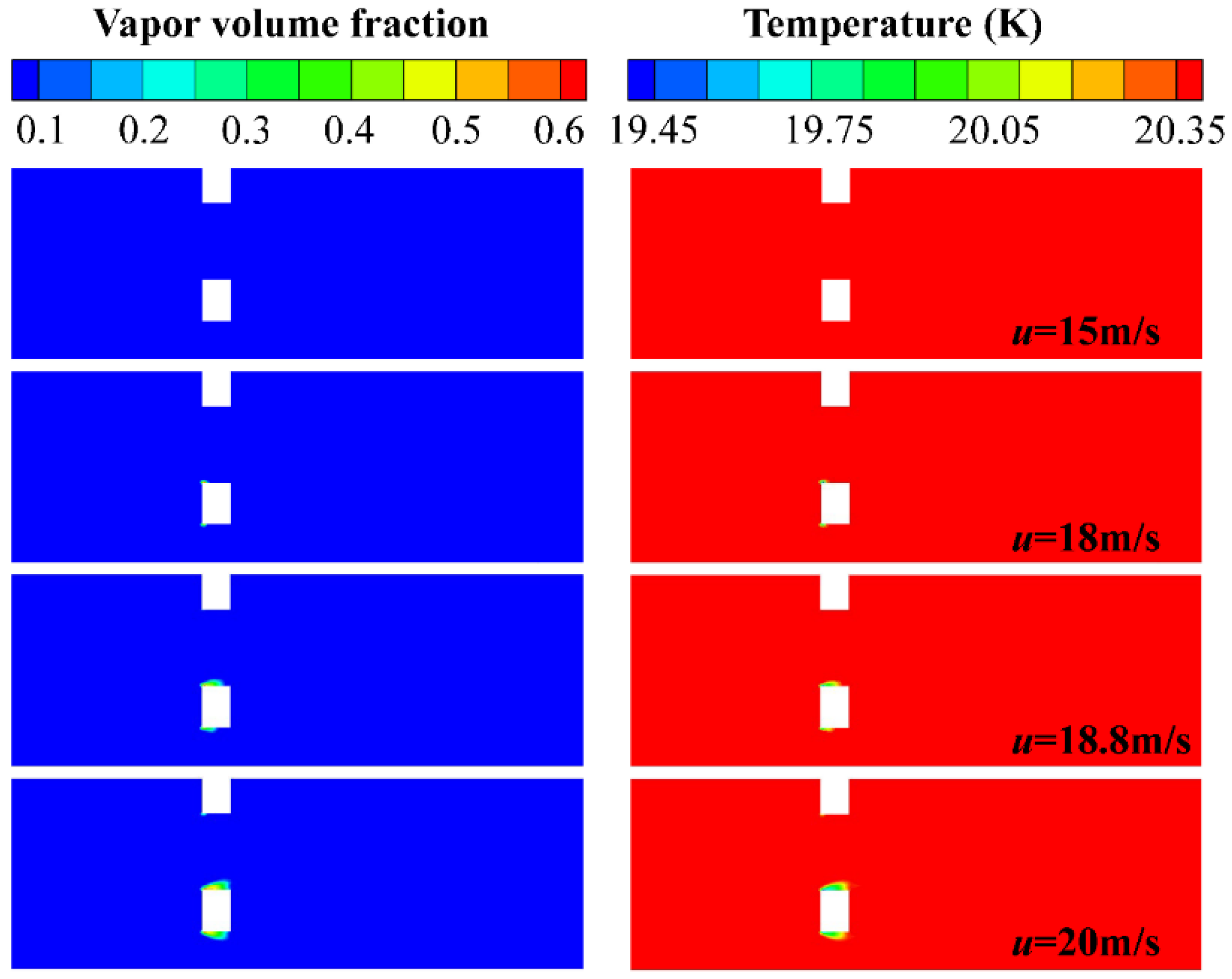
Table 1.
Involved physical properties of water, LN2, and LH2 at standard pressure [5].
Table 1.
Involved physical properties of water, LN2, and LH2 at standard pressure [5].
| Physical properties | H2O | LN2 | LH2 |
| Temperature (K) | 300 | 77.36 | 20.37 |
| Density (kg/m3) | 997 | 807 | 71 |
| Saturation pressure (Pa) Dynamic viscosity (10-4 m2/s) |
3537 0.01004 |
101384 0.00199 |
101324 0.00188 |
Disclaimer/Publisher’s Note: The statements, opinions and data contained in all publications are solely those of the individual author(s) and contributor(s) and not of MDPI and/or the editor(s). MDPI and/or the editor(s) disclaim responsibility for any injury to people or property resulting from any ideas, methods, instructions or products referred to in the content. |
© 2025 by the authors. Licensee MDPI, Basel, Switzerland. This article is an open access article distributed under the terms and conditions of the Creative Commons Attribution (CC BY) license (http://creativecommons.org/licenses/by/4.0/).
Copyright: This open access article is published under a Creative Commons CC BY 4.0 license, which permit the free download, distribution, and reuse, provided that the author and preprint are cited in any reuse.


