
Submitted:
18 January 2025
Posted:
21 January 2025
You are already at the latest version
Abstract
To gain a more detailed understanding of the specific properties of complex shaped technical aerosols, it is necessary to measure more than one equivalent quantity. This paper presents a new method to determine the two-dimensional distribution of two distinct particle properties: the Centrifugal Differential Mobility Analyzer (CDMA). It is capable of measuring both, the mobility and the Stokes equivalent diameters as a comprehensive two-dimensional distribution. To achieve this, the techniques of the Aerodynamic Aerosol Classifier and the Differential Mobility Analyzer are combined in a single device. The inversion of the data is conducted using the projection onto convex sets approach. For a valid interpretation of the results, it is essential to comprehend the operational mode of the CDMA including a profound knowledge about particle transport in the classifying section as well as in the inlet and outlet regions. Consequently, this paper presents some flow simulations of the measuring device and detailed experimental investigations of the transfer functions to evaluate a first prototype of this device. The resulting findings serve as a foundation for the calculation of a fully two-dimensional distribution with regard to the mobility and Stokes equivalent diameter. This is demonstrated with some exemplary measurements, e.g. of aggregates at different sintering stages.
Keywords:
Centrifugal Differential Mobility Analyzer
; 2D-Measurements
; particle characterization
; moving reference frame CFD-simulation
; calculation of transfer funnctions
1. Introduction
Advances in technology nowadays often require the availability of increasingly sophisticated methodology. Regarding the characterization of nanoparticles, the small dimensions drastically limit their direct investigation. Therefore, in most cases, an equivalent size is established. An equivalent diameter for example, is the diameter, a spherical particle would have regarding the obtained feature (e.g. electrical mobility). Naturally, this results in manifold potential equivalence values. To gain a more comprehensive understanding of a particle collective, it is possible to simultaneously determine multiple quantities. This can be achieved, for instance, using scanning electron microscopy (SEM) or tandem configurations, where one equivalent size can be initially measured and subsequently another one. However, these methods are complex in terms of the equipment which makes them expensive, require a high degree of expertise, or have poor statistical properties regarding sample size. To facilitate the combined measurement of multiple quantities, the CDMA (Centrifugal Differential Mobility Analyzer) was developed. The CDMA is a combination of an Aerodynamic Aerosol Classifier (AAC) ([1] and a Dynamic Mobility Analyzer (DMA) [2], which enables the simultaneous measurement of the equivalent mobility diameter and the equivalent Stokes diameter, thus yielding a two-dimensional distribution of these two variables. Subsequently, additional parameters, such as the effective density or the fractal dimension, can be determined, giving information on particle shape as well [3,4,5].
2. Theoretical Fundamentals
Like the DMA and AAC, the CDMA is composed of two concentric cylinders arranged concentrically, guiding a sheath air flow (c.f. cross-section of the CDMA in Figure 1). When an aerosol volume flow is applied to the inner cylinder (c.f. Figure 1, detail A), the particles are moved toward the outer cylinder by centrifugal and electrical forces. At the end of the classification chamber, (c.f. Figure 1, detail B), the particles are sampled, so that particles matching the predetermined properties are counted. Assuming Stokes’ drag force, the force equilibrium results in:
represents the particle charge, E denotes the electric field magnitude, is the particle mass, represents the centrifugal acceleration, denotes the dynamic viscosity, is the mobility diameter, denotes the particle drift velocity, and Cu is the Cunningham slip correction factor. The deterministic description of the particle path is achieved by rearranging and integrating equation (1).
U represents the voltage, denotes the rotational velocity, and are the outer and inner radii, is the radius at which the particle enters, y is the position of the particle in the direction of the length L, is the sheath air volume flow, is the aerosol volume flow, is the particle relaxation time and Z is the particle mobility. With
and
the particle path for each variable can be calculated from the volume flow ratio and the applied rotational velocity and voltage. is the mobility required for a particle entering at the center of the aerosol inlet to be sampled exactly at the center of the outlet [6]. describes the same behavior, but for the relaxation time [1].
is the particle density, is the Stokes equivalent diameter, n is the number of charges carried by a particle, e is an elementary charge and is the excess gas volume flow. Relating the particle properties Z and to the characteristic mean values of the actual operation point and lead to the normalized mobility or the normalized particle relaxation time, respectively.
For further information, see [7].
3. Design
Figure 1 shows a cross-section of the CDMA. The aerosol is fed from the left side, enters through the center bore, and flows through a small gap to the inlet of the classification channel A. The sheath air is fed between two ferrofluidic seals on the left side. Then it passes through 8 axial holes into the CDMA, where it mingles with the aerosol volume flow at A. Together the flows pass through the classification zone. At point B, the excess volume flow continues the inner cylinder, flows to the center and exits through a center bore on the right side. The sample air is extracted in the radial direction at point B. Then, the sample flows through small channels until it leaves the CDMA through a small hole between the ferrofluidic seals on the right side. Voltage can be applied through a carbon-sliding contact on the outer cylinder, the speed is applied by a belt drive mounted on the left side [7].
4. Numerical Flow Simulations
CFD simulations were performed under the assumption of incompressible flow using the k- SST-model with OpenFOAM. Since there are eight symmetrically arraanged inlet pipes for the sheath air, the flow domain can be reduced to an eighth of the whole geometry, as shown in Figure 2.
The symmetry interfaces were defined as periodic interfaces, so fluxes across the interfaces were admitted. The boundary condition at the walls is a zero-slip boundary condition (Dirichlet boundary condition for the velocity). The aerosol inlet, sheath air, and excess air are also defined as Dirichlet boundary conditions. In this case, the velocity is not set to zero but to values that correspond to the desired flow rate in or out of the domain at the respective in- or outlet. The aerosol inlet and the excess air outlet have a plug-flow velocity profile, while the inlet of the sheath air is modeled with a fully developed laminar flow. The sample outlet is defined by the Neumann condition; thus the mass balance is always maintained.
The rotation is implemented by a single rotating frame approach, using the ’SRFSimpleFoam’ solver to calculate the velocity fields. The flow ratio (, ) is considered in the following simulation results.
4.1. Flow Behavior Without Rotation
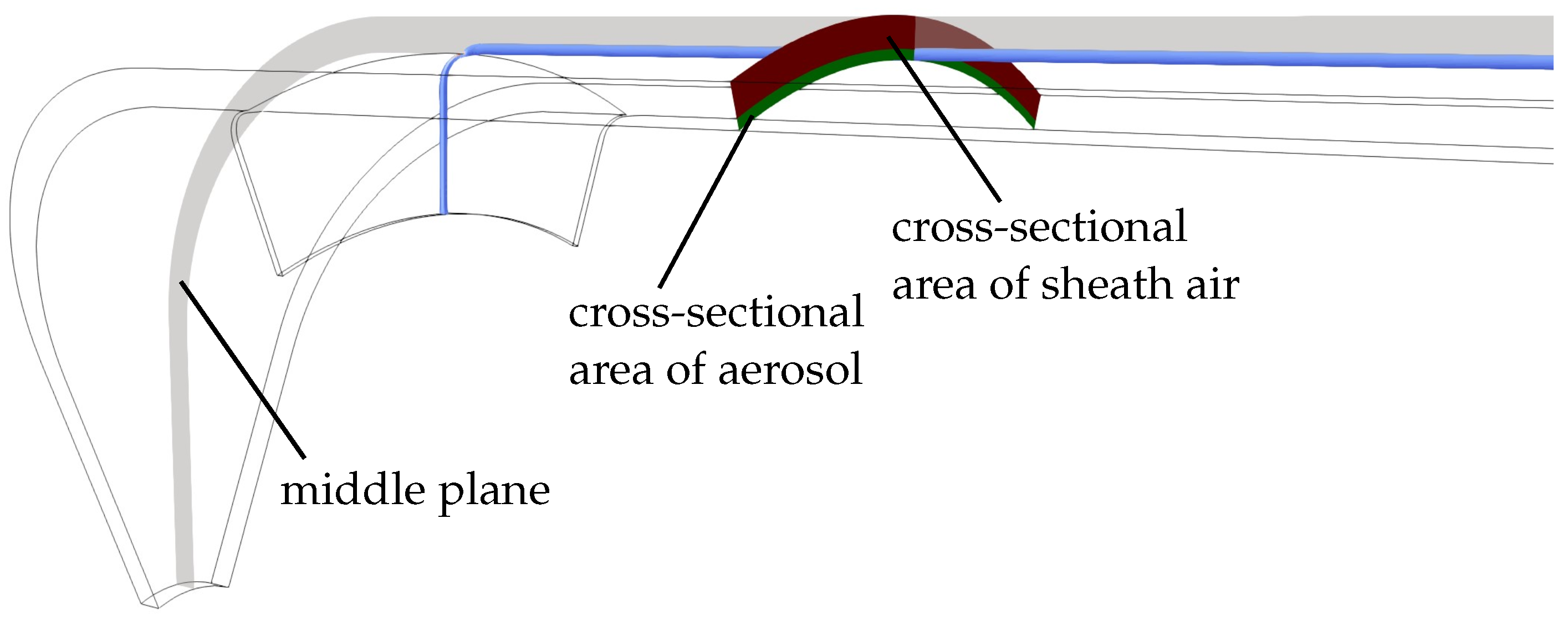
To investigate the radial symmetry of the flow, Figure 3 shows the flow pattern at different positions. Here, x is the absolute position in axial direction, where is at the inlet of the sheath air. For reasons of clarity the velocities in axial direction in the highlighted planes are color coded. On the right side the calculated vectors are shown exemplary to emphasize that there is only flow in the axial direction. At the axial coordinate , the deflection of the sheath air ends. The second plane from the left is located directly before the aerosol joins the sheath air. It can be observed that the flow profile is symmetrical across the gap width, with no significant deviations in the circumferential direction. Additionally, there is only a slight change in the axial direction. However, due to the limitations of this representation, it is challenging to accurately quantify the data. Figure 4 provides a more detailed illustration of the axial velocity at the center of the gap, which allows for a more precise analysis of the circumferential direction (white lines of Figure 3).
At , which is upstream of the aerosol inlet, the velocity distribution is slightly irregular, due to the influence of the deflection arc. However, immediately at the beginning of the transfer domain at , the velocity distribution becomes quite regular. Further downstream, when the aerosol is inserted, the velocity in the axial direction increases because the volumetric flow rate is higher while the cross-section remains constant. Because there is no change in the circumferential direction, it is valid to represent the velocity in the axial direction in the transfer domain by using velocity values from the middle plane of the investigated flow domain if no rotation is applied.
Figure 5 shows the streamlines at for this middle plane. There appears to be no cross mixing, but the streamlines of the particle laden flow widen to a certain extent. There are two reasons. First, the flow has a little radial component since the outlet/inlet is very short. Second, the CDMA is constructed that for , so the two streams would perfectly fill the space. A of means that there is relatively more of that needs to occupy more space. Additionally, this will be increased through the presence of a flow profile, because if there is a laminar flow profile over the gap, the velocity in the middle is much higher, so there is more fluid transported over time.
4.2. Flow Behavior with Rotation
Figure shows the axial flow profiles in the circumferential direction analogous to Figure 4, but for certain values of rotational velocity of the outer cylinder. It can be observed that, at low speeds, the flow profile distribution over the circumference is homogeneous. At higher rotational speeds, a larger flow length is required until a homogeneous flow profile is achieved over the circumference. The axial velocity also increases with increasing speed, at least during the initial phase of the classification zone (x = 0.151 m). This can be attributed to a higher volume flow at the inner boundary due to the elevated pressure at the outer boundary. Consequently, the resulting velocities are higher. Although an inhomogeneous velocity profile was identified over the circumferential direction, the difference in flow velocity at each location was found to be insignificant (with a maximum deviation of around the value at ). Consequently, only the results from the center plane are discussed below.
The flow of the sheath air through the arc ahead of the transfer domain is displayed at a rotational speed of in Figure 6. The displayed vectors represent the relative velocity and are directed in the opposite direction to the rotation. This is because the flow continuously experiences a higher circumferential velocity while traveling in the positive radial direction. While having only a density of about , air experiences mass inertia and cannot instantly adopt its flow direction to the increased circumferential velocity. Thus, the flow appears to move against the direction of rotation based on the relative velocity. At the end of the deflection arc, the flow of the sheath air remains at the respective level of circumferential velocity and eventually adopts its flow direction in the axial direction (right hand side, Figure 6).
The resulting velocity vector needs more traveling distance to point only in the axial direction. This relation is displayed in Figure 7. The vectors of the relative velocity on the middle plane are displayed from a top-down perspective for different rotation numbers.
With increasing rotational speed, the pressure increases at the outer wall when the sheath air arc is left. In Figure 8 axial velocity fields of the cases for 0, 475, and 2000 rpm are compared.
It can be observed that the effective flow cross-section for the flow in the axial direction decreases with increasing rotational speed. This resulted in a shifted velocity profile toward the inner wall of the transfer domain and higher peak velocities. Downstream in the axial direction, the effective cross-section widens up to the geometrically available cross-section. This results in a more symmetric profile for the axial velocity.
5. Derivation of Ideal Transfer Functions from the CFD Simulation
To investigate the influence of the flow profile on the classification the transfer function was derived directly from CFD data. The determination of a transfer function for specific CDMA operating parameters (at fixed voltage and velocity) is a stepwise process. First, for a given particle size (e.g. the smallest to be investigated), the entry point of the particles is varied, and the corresponding trajectories are calculated to see which particles will reach the classification zone. Second, the particle size is varied according to a given particle collective. The transfer probability for one particle size is then given by the number of successfully traversed particles divided by the number of entry points :
The particle size can then be converted into the mobility Z, particle relaxation time or their normalized values (), respectively.
The particle trajectory was calculated using CFD data (c.f. Figure 9). A virtual time step was defined for a trajectory. For every node (black points in Figure 9) the velocity data is known. The algorithm searches the nearest data point to the particle and uses the velocity given there to calculate the way the particle is traveling in axial direction. In radial direction the velocity is computed neglecting diffusion and inertia of the particle, the way of the particle in radial direction could be calculated using the particle size, radial position, and operating parameters of the CDMA (c.f. equation (2)).
Figure 10 shows successfully sampled particle trajectories (green) and deposited ones. It is obvious that the resolution of the simulation depends on the number of streamlines, the duration of the virtual time steps and the number of particle sizes investigated. However, this increases with computational cost, thus a compromise must be made.
5.1. Ideal Transfer Function
To compare the simulated results with theoretical values, we use ideal transfer functions. The ideal two-dimensional transfer function was derived from streamline functions by Rüther (forthcoming2).
is the ratio of aerosol volume flow to sheath air volume flow , is the ratio of the gap width to the mean radius, is the ratio of the inner radius to the outer radius and A is a substitution.
This results in a two-dimensional distribution, displayed in Figure 11. As the computing power would be too immense for a complete two-dimensional simulation as described in Section 5 only the transfer functions for and (red, dashed lines) and the transfer function for spherical particles (red solid line) are investigated.
5.2. Simulated Transfer Functions for and
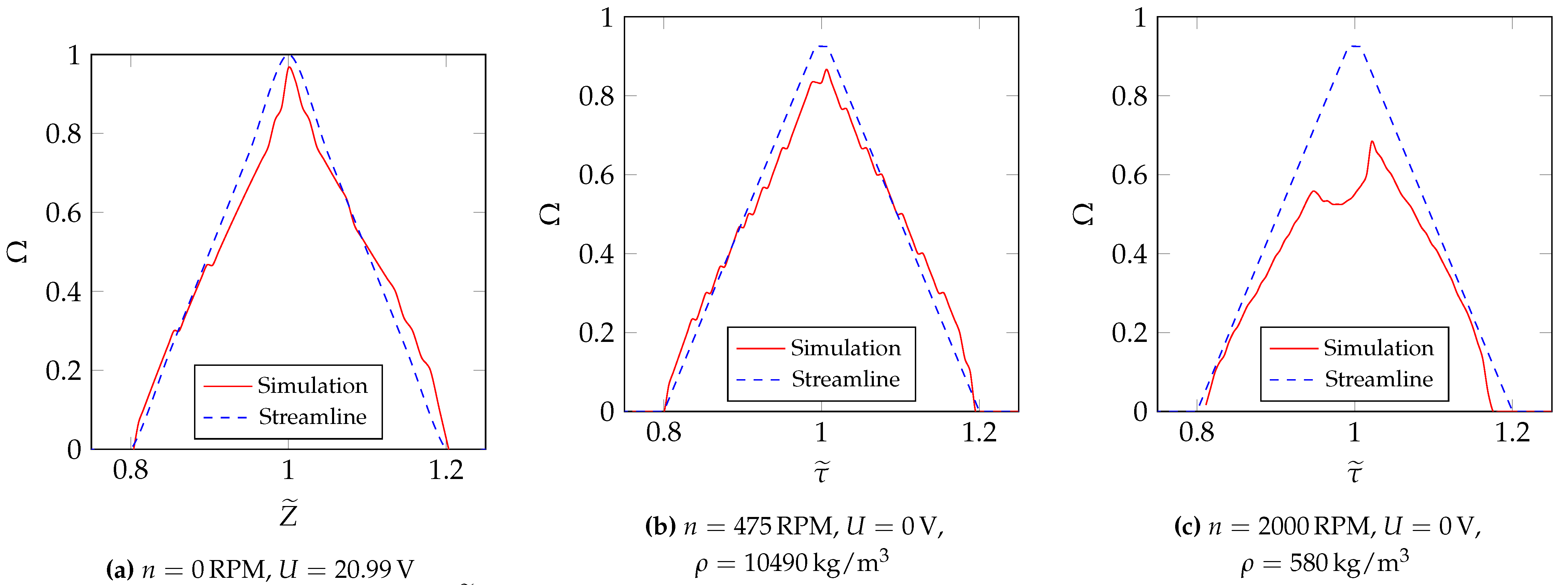
The transfer functions illustrated in Figure were calculated at different densities. and are unity at a particle size of . It is evident that the simulation results exhibit several discernible stages, which can be attributed to the limited resolution, particularly the restricted number of particle trajectories per particle size. An investigation of the pure electrical mode (see Figure ) revealed a high degree of agreement between the transfer functions. The minor discrepancies can be attributed to the flow field. Figures and illustrate the transfer functions at different speeds in purely rotational mode. The transfer functions exhibit a high degree of agreement for the case of (see Figure ). The transfer function is slightly lower, indicating a slightly higher separation. As the speed increases (cf. Figure ), the relative position of the transfer function remains consistent, although the initially distorted flow profile increases the likelihood of particle separation.
5.3. Simulated Transfer Functions for Different CDMA Operating Parameters
To extend the investigation of the transfer functions not only for the transfer functions at and , the combination of applying both, voltage and rotational velocity is examined, too. To simply the two-dimensional transfer function to a one-dimensional transfer function, which then can be investigated, perfectly spherical particles are used. Here, following dependency emerges (see red solid line in Figure 11):
Varying the operating parameters results in a shift of that line, resulting in the transfer functions shown in Figure . The simulated transfer functions are again very close to the ideal transfer functions but are smaller in height.
This indicates that the transfer functions derived from the simulation are accurately represented by the theoretical calculation. Furthermore, the results demonstrate that a laminar flow profile within the CDMA has no significant impact on the transfer behavior. At higher speeds, distortion of the transfer function occurs when the flow profile is not yet fully developed.
A significantly greater influence is observed when the boundary condition of a constant particle flow density at the inlet is assumed by assuming a constant particle flow density and a laminar flow profile at the aerosol inlet. This behavior is already described in (Rüther, forthcoming2), but could also be supported by a simulation in a subsequent study.
6. Measurement of Transfer Functions
Consequently, after the simulative validation of the ideal transfer functions, the next step must be experimental validation.
6.1. Theory
Like shown in Rüther et al. ([7]) tandem setup comprising a DMA and a CDMA is employed to determine the transfer functions (c.f. Figure 12). Following the assumption of a broad distribution of the test aerosol, the ratio of the number concentrations ( and after the CDMA classification) can be described as follows [8]:
The transfer functions in general are well described by Gaussian functions (Rüther, forthcoming2). being the parameters of the Gaussian function, the transfer function of the pre-classifying DMA , and the transfer function of the CDMA , can be described as follows:
Thus, equation (15) can be simplified analogous to [7]:
This means that measuring the ratio while varying the voltage or rotational velocity of the CDMA (i.e. varying the ), makes it possible to determine the transfer function by simply fitting a Gaussian function to the measurement data [7].
However, for this purpose, the transfer function of the pre-classifying DMA must be precisely determined. The exact approach to achieve this is described in Appendix B, so that and are determined as follows:
This procedure for determining the transfer function of a DMA-DMA setup can be applied to a DMA-AAC setup as well. In the case of spherical particles, the mobility of the first DMA can be converted into the particle relaxation time. Defining the transfer functions as follows:
The following parameters can then be determined by applying equation A1.
These values can be used to calculate the transfer functions for the CDMA according to equation 17.
6.2. Production of the Test Aerosol and Measurement Setup
A method for producing an aerosol of a relatively immutable, broad particle size distribution over an extended period was developed using a setup comprising two hot-wall reactors with an agglomeration tube positioned between them (see Figure 12). Silver is is melted and evaporated at a temperature of within the front hot-wall reactor. The air saturated with silver is extracted from the hot-wall reactor via an air flow. The flow rate () was regulated by a mass flow controller (MFC). During the cooling phase, the solution becomes supersaturated, resulting in the formation of silver particles. Subsequently, larger agglomerates are formed in the agglomeration tube, which are ultimately sintered into spherical particles in the second hot-wall reactor at .
Subsequently, the spherical particles are pre-classified in a DMA, which is set to a specific mobility value. The aerosol then passes through valve . Opening and simultaneously bypasses the CDMA, allowing the number concentration to be determined directly by the CPC. Conversely, when both valves are closed, the aerosol passes through the CDMA, which was programmed to run sweeps for the voltage and the rotational velocity. This allows the number concentration to be determined as a function of the operating parameters .
6.3. Determination of the Transfer Function Parameters for and at Different -Values
Figure illustrates the parameters of the CDMA transfer function over a range of operational parameters for . Figure illustrates the parameters of the CDMA transfer function over a range of operational parameters for . Considering the influence of diffusion, particularly in the case of the CDMA geometries (where the gap width is small, thereby necessitating a substantial diffusion component), the diffusion-related transfer functions, can be calculated in (Rüther, forthcoming2). Using these influences adjusting the measurement values. Additionally, Rüther et al. ([7]) demonstrated that at specific points in the CDMA, increased separation occurs due to peak values in the electric fields and the centrifugal field at the sample outlet. These values were also calculated and the measured values corrected accordingly.
Besides these adjustments, a direct relation between particle size and deposition is evident in Figure . Moreover, a reduction in deposition is evident at elevated aerosol volume flows. It is noteworthy that values exceeding 1 were observed, which can be attributed to potential measurement errors or inaccuracies in the determination of the transfer function of the pre-classifying DMA.
Moreover, the width of the transfer function is nearly identical to the calculated ideal width (cf. Figure ). However, the measurement series for exhibits a slight elevation for particles, which can also be attributed to measurement errors. This is because only a negligible number of particles were counted at , as this was at the edge of the particle size distribution of the test aerosol.
The width of the transfer function (Figure ) is comparable to the results obtained from the DMA experiments, which are presented in Figures to .
The transfer functions for are illustrated in Figure . It is important to note that for , there is no measurable transfer function. This is due to particle separation occurring at the outlet due to the prevailing centrifugal forces. Thus, each measurement series comprises only two data points [7].
Figure illustrates the maximum height of the transfer functions. Despite the corrections, the transfer function remains dependent on the particle size and the prevailing flow conditions. This finding is particularly relevant in the context of rotational operation, because even small imperfections, such as deviations in production, a non-concentric alignment of both cylinders, and similar factors have a greater impact on the flow field, generating this dependency. The measurement was conducted over the entire CDMA (including transport to and from the measurement gap), thus precluding the possibility of correcting all undetermined losses. However, no direct correlation could be established, and thus, no equivalent loss length for diffusion, as would be present when flowing through a pipe, could be determined.
Figure illustrates the width of the transfer function. The measured values displayed do not exhibit a correlation with the beta values as the range of variation is too big. This can be attributed to the inaccuracies and the big losses of the CDMA system. In comparison to , a notable shift in the transfer function (c.f. Figure ) is present. This indicates a dependency to particle size, volume flows or rotational speed.
6.4. Determination of the Transfer Function Parameters for and at
Since a complete investigation of all parameters would be very time-consuming, it is better to focus on a more detailed investigation of the targeted operating conditions ( at ). As part of this investigation, the transfer functions for particles of varying sizes are measured once more under the aforementioned conditions. The resulting data is presented in Figure .
After correction, it can be observed that the height of the transfer functions (see Figure ) is highly stable for all particle sizes investigated and exhibits a similar magnitude for both operating modes. It is notable that the width of the transfer functions exhibits a slight upward deviation for larger particles, which can be attributed to the relatively low particle number for particles exceeding . Moreover, the correlation between displacement and particle size, speed, and voltage can be determined.
The results are then transferred to the actual measurement operation and the kernel matrix is calculated (see (Rüther, forthcoming3)). This is achieved by forming an average value from all measured values with regard to the height, using the ideal width as the basis for the width. The shift can be corrected by a straight line drawn through the measured values.
7. Measurement Results and Analysis of Two-Dimensional Size Distributions for Different Sintering Stages of Silver Nanoparticles
The results from Section 6 are now employed in the calculation of the kernel matrix, which is analogous to that described by (Rüther, forthcoming3). Subsequently, the two-dimensional distribution is calculated using a POCS algorithm (Rüther, forthcoming3).
7.1. Production of the Aerosol and Measurement Setup for Two-Dimensional Distributions
The first measurements of a two-dimensional particle size distribution are carried out using the same test aerosol from Section 6.2 but with no pre-classifying DMA. Figure 13 shows the setup. In this study, the sintering stage should be influenced by the temperature of the sintering furnace. Here, temperatures of , , , , , and are used.
7.2. Derivation of Further Properties
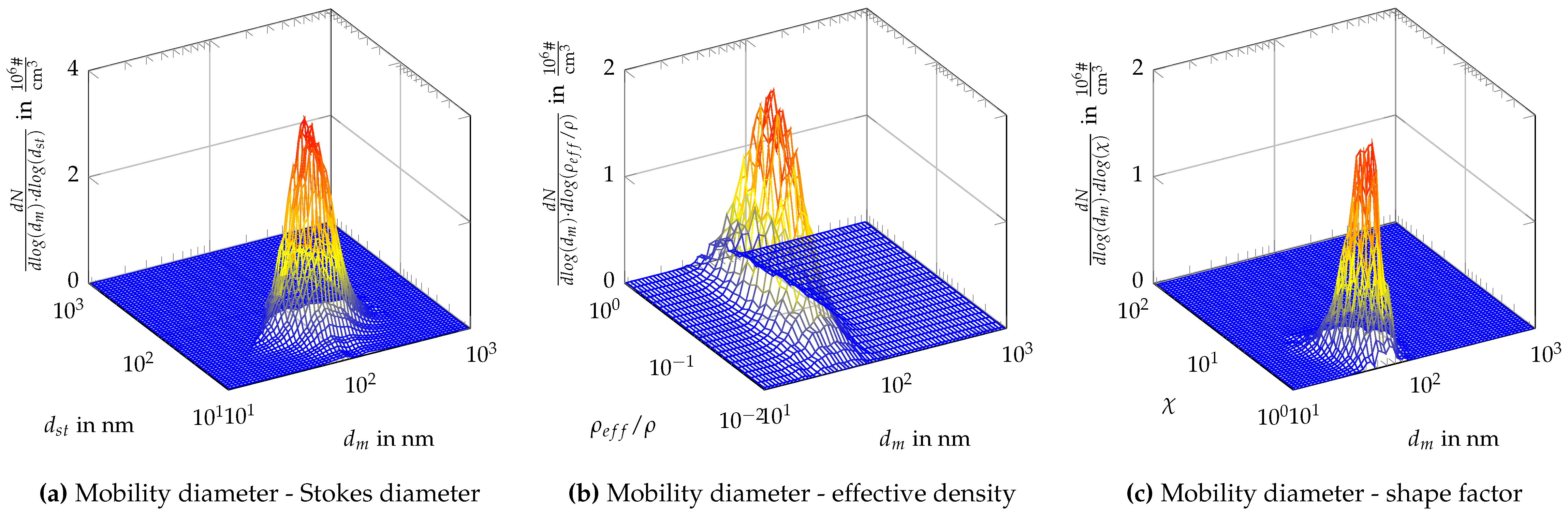
From the two-dimensional distribution of the mobility and Stokes diameter, it is possible to derive other quantities like the aerodynamic and volume equivalent diameters, the effective density or the shape factor [9].
These relations are used to calculate further the two-dimensional distributions which are displayed and discussed.
7.3. Measurement Results
Figure to show the two-dimensional distributions of the forementioned quantities at different sintering temperatures. At high sintering temperatures, the relative effective density and shape factor for each particle are close to 1. The -distribution shows a bi-sectional distribution as we obtain almost perfectly spherical particles. For lower sintering temperatures, the relative effective density becomes lower, and the shape factor becomes larger, showing more irregularly shaped particles (c.f. Figures to , for more sintering stages in between). The use of this additional information about the particle shape could lead to a better understanding of the process. So the absorption or reaction coefficients can be manipulated trough the particle production process, for generating more effective particles.
8. Conclusions
The proposed methodology for determining two-dimensional property distributions has significant potential for both research and industrial processes. With these additional insights, the behavior of the particle systems can be more comprehensively understood. The Centrifugal Differential Mobility Analyzer can measure two-dimensional distributions regarding the mobility and Stokes diameter and thus enabling the investigation of the spatial distribution of different other characteristic property values. The functionality of the prototype was validated and then meticulously characterized to identify potentials for further improvements. Nevertheless, it is feasible with high accuracy to determine the actual transfer functions, thereby enabling data inversion on this basis. The data inversion is highly robust and yields plausible results (Rüther, forthcoming3), that can be converted into further property distributions. In comparison with one-dimensional measurement techniques, the CDMA offers a substantial increase in the amount of information obtained. Consequently, the next step must be the construction of an enhanced version, which will exhibit significantly fewer losses and therefore provide significantly better measurement values [7], reduce the diffusion by using a lager gap (Rüther, forthcoming2) and enhance the flow field within the CDMA at enhanced rotational speeds. The implementation of the scanning mode enables a substantial reduction in the measurement time, thereby rendering the entire measurement process less susceptible to errors i.e. fluctuations at the test aerosol generation process. Subsequent investigations should also cover the further validation of results, such as the actual particle sizes and effective density, using scanning electron microscopy (SEM) images. If a known particle shape is known, it is feasible to determine the charge distribution and the Cunningham slip correction, thereby establishing a novel methodology for determining these variables, particularly for non-spherical particles. Furthermore, combining the CPC with a Faraday-Cup-electrometer result in more information and thus in the stabilization of the data inversion. The presented study focuses on the determination of particle shape. Therefore, it is essential to determine the density with a high degree of precision. However, in the case of unknown particle systems, no information that allows the actual shape to be determined is available. Integration with additional measurement systems could enable access to a three-dimensional distribution of properties. For instance, it may be feasible to examine the scattered light behavior of particles in conjunction with the CPC or to integrate mass spectrometry.
Conflicts of Interest
The authors declare no conflict of interest.
Abbreviations and Nomenclature
Abbreviations
The following abbreviations are used in this manuscript:
| CDMA | Centrifugal Differential Mobility Analyzer |
| DMA | Differential Mobility Analyzer |
| AAC | Aerodynamic Aerosol Classifier |
| CPC | Condensation Particle Counter |
| lpm | liters per minute |
| RPM | Rounds per minute |
| MFC | Mass-flow Controller |
Nomenclature
| particle charge | |
| E | electric field |
| particle mass | |
| centrifugal acceleration | |
| dynamic viscosity | |
| n | number of particle charges |
| particle relaxation time | |
| nominal particle relaxation time | |
| normalized particle relaxation time | |
| particle mobility | |
| nominal particle mobility | |
| normalized particle mobility | |
| mobility equivalent diameter | |
| aerodynamic equivalent diameter | |
| stokes equivalent diameter | |
| volume equivalent diameter | |
| diameter of a sherical particle | |
| aerosol volume flow | |
| sheath air volume flow | |
| sample volume flow | |
| excess air volume flow | |
| L | length of the CDMA transfer path |
| inner radius | |
| maximum radius at which the particles enter | |
| outer radius of the aerosol air streamlines | |
| inner radius of the sampling air streamlines | |
| particle drift velocity | |
| y | length coordinate in axial direction |
| Cunningham slip correction factor | |
| U | voltage |
| particle density | |
| virtual assumed density of | |
| effective density | |
| angular speed | |
| transfer function | |
| ratio of to | |
| ratio of the gap width to the mean radius | |
| ratio of to | |
| total number of simulated streamlines | |
| number of sucessfully traversed streamlines | |
| fit parameters for the height of a Gaussian function | |
| fit parameters for the width of a Gaussian function | |
| fit parameters for the shift of a Gaussian function | |
| width of the transfer function | |
| shape factor |
Appendix A. Further Illustration of the CFD Simulation
Figure A1.
Schematic drawing of the flow sections and the middle plane
Appendix B. Transfer Function Parameter Determination
As it is very important to know the transfer function of the pre-classifying DMA precisely when measuring the transfer function via a tandem setup (see equation (15)), this section describes how this transfer function can be determined in advance.
For this purpose, three identical DMAs (Long DMA TSI 3081) were measured in each constellation in the tandem setup. The aerosol used was a silver aerosol, which was produced as in section 3 (please mention that equation (15) is only applicable for brought particle size distributions at the inlet of the first DMA. Otherwise, the distribution must be included in the calculation). Assuming that the transfer function can be well described by a Gaussian function (Rüther, forthcoming2) for two identical DMA’s . Since is the varried parameter for the data points to fit on, in this special case, must be set to one, and the resulting shift then is twice as high. Thus, simplify equation (17) for two identical DMA’s results in:
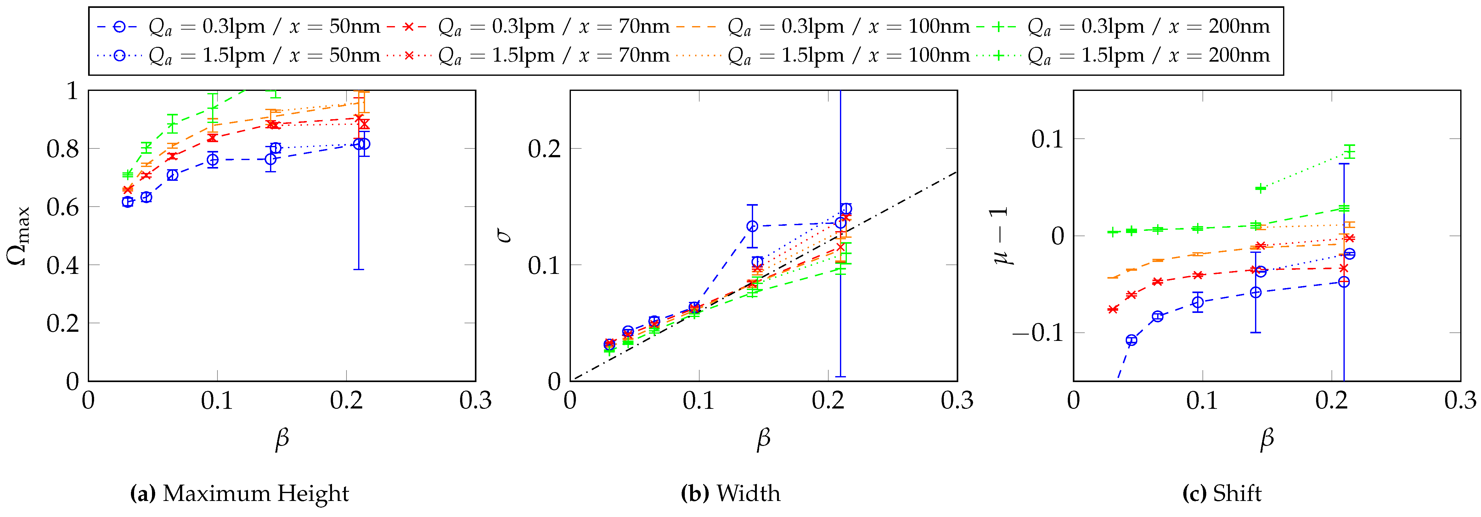
To obtain comparative values that were as valid as possible, the aerosol volume flow rate was varied to 0.3 and 1.5 lpm, as well as the sheath air volume flow rate was varied to different values. This was done to ensure the most accurate and valid results possible. This method enabled the analysis of different beta values. The series of measurements were conducted at particle sizes of 50, 70, 100, and 200 nm. For every measuring point, the mean value was calculated from three individual measurements, resulting in a measured parameter set for every setting (see Figure ). To determine the characteristic parameters of every DMA, the mean value of was first determined for every DMA-DMA combination. The c has a linear dependency to so that a linear regression is applied to obtain a regression constant for every combination, so that . Table A1 lists the values for and if the tandem setup consists of two identical DMAs. It can be seen that the values for the combinations differ from each other, but there is some regularity.

Table A1.
Values for and assuming two identical DMA’s in a tandem setup.
| DMA combination | 1-2 | 1-3 | 2-1 | 2-3 | 3-1 | 3-2 |
|---|---|---|---|---|---|---|
| 0.6778 | 1.0173 | 0.6964 | 1.0443 | 0.8622 | 0.8950 | |
| 1.0282 | 1.0568 | 1.0261 | 1.0504 | 0.9900 | 0.9891 |
To obtain the real parameters for every DMA, a system of equations is required. For the widths of the transfer function, we follow by comparing the coefficients of equations (A1) and (17):
And therefore:
Thus, it is possible to set up a system of equations, where is the solution vector for each combination, while and are the unknown variables.
The same can be done for :
Here, is the solution vector. Since the DMA’s were interchanged in every direction the system of equations was overdetermined, so the solution was a least squares regression.
The height a of the transfer function for the pre-classifying DMA is not important, because it is omitted from equation (17). This yields the parameters taken for the DMAs as shown in Table A2.
Table A2.
Parameters of the analysed DMA’s.
| DMA | 1 | 2 | 3 |
|---|---|---|---|
| k | 0.5732 | 0.5988 | 0.7818 |
| 1.0154 | 1.0117 | 1.0080 |
Here, it is shown that DMA1 and DMA2 are near, but DMA3 has a much higher value for k, which yields in broader transfer function. This is also proved in Figures to , where it can be seen that for the figures where DMA3 is the second DMA, is much higher, while for the other diagrams the width is around the theoretically ideal line (black dashed line).
Moreover, the maximum height of the transfer functions is decreasing with decreasing values for . This is because, for smaller transfer functions, the influence of diffusion is increasing. There is also a clear tendency from small to large particles at the maximum height, which is caused by diffusion. For some measurement points the maximum height exerts one. Here, DMA3 is the pre-classifying DMA. This indicates that there are discrepancies in the determination of the parameters or measurement errors.
The shift does not seem to have major dependencies on the -values but seems to be influenced by the particle size or the volume flows itself. This is caused by deviations in the applied voltage of the system.
DMA1 appears to have the best properties, thus it was selected as the pre-classifying DMA for the CDMA transfer function measurements.
Figure A2.
Measured transfer function parameters of the the DMA combination 1-2, with 95% confidence interval derived out of three samples.
Figure A2.
Measured transfer function parameters of the the DMA combination 1-2, with 95% confidence interval derived out of three samples.
Figure A3.
Measured transfer function parameters of the the DMA combination 1-3, with 95% confidence interval derived out of three samples.
Figure A3.
Measured transfer function parameters of the the DMA combination 1-3, with 95% confidence interval derived out of three samples.
Figure A4.
Measured transfer function parameters of the the DMA combination 2-1, with 95% confidence interval derived out of three samples.
Figure A4.
Measured transfer function parameters of the the DMA combination 2-1, with 95% confidence interval derived out of three samples.
Figure A5.
Measured transfer function parameters of the the DMA combination 2-3, with 95% confidence interval derived out of three samples.
Figure A5.
Measured transfer function parameters of the the DMA combination 2-3, with 95% confidence interval derived out of three samples.
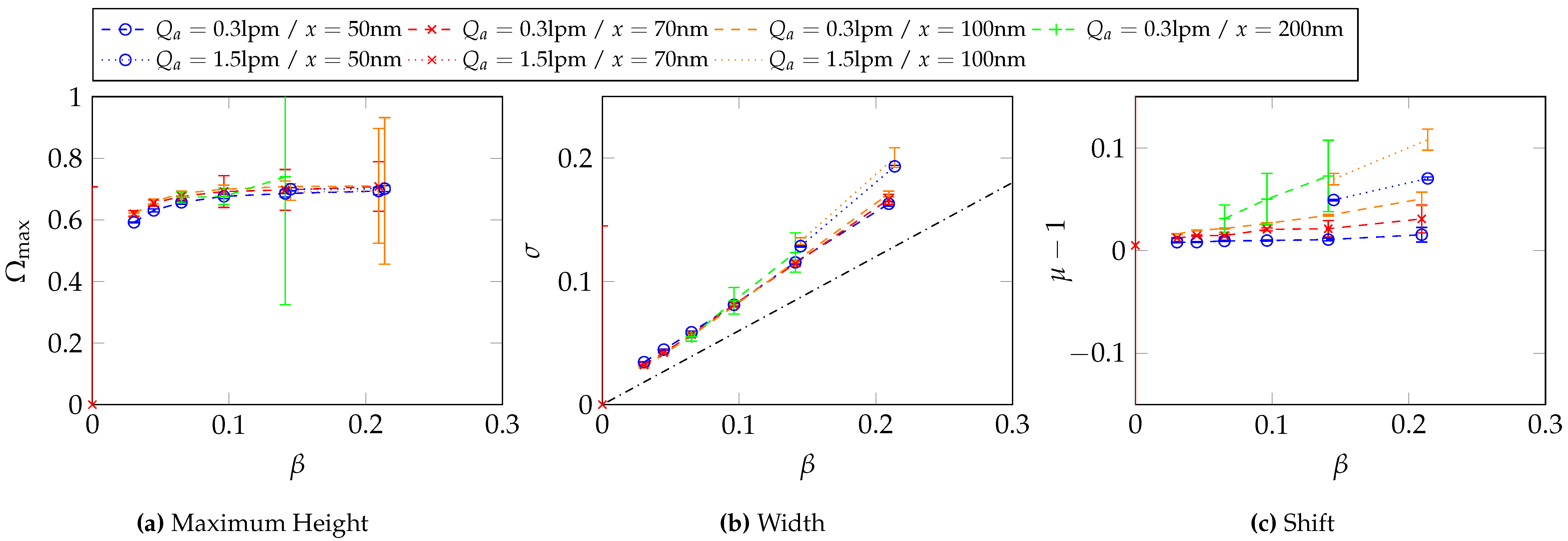
Figure A6.
Measured transfer function parameters of the the DMA combination 3-1, with 95% confidence interval derived out of three samples.
Figure A6.
Measured transfer function parameters of the the DMA combination 3-1, with 95% confidence interval derived out of three samples.
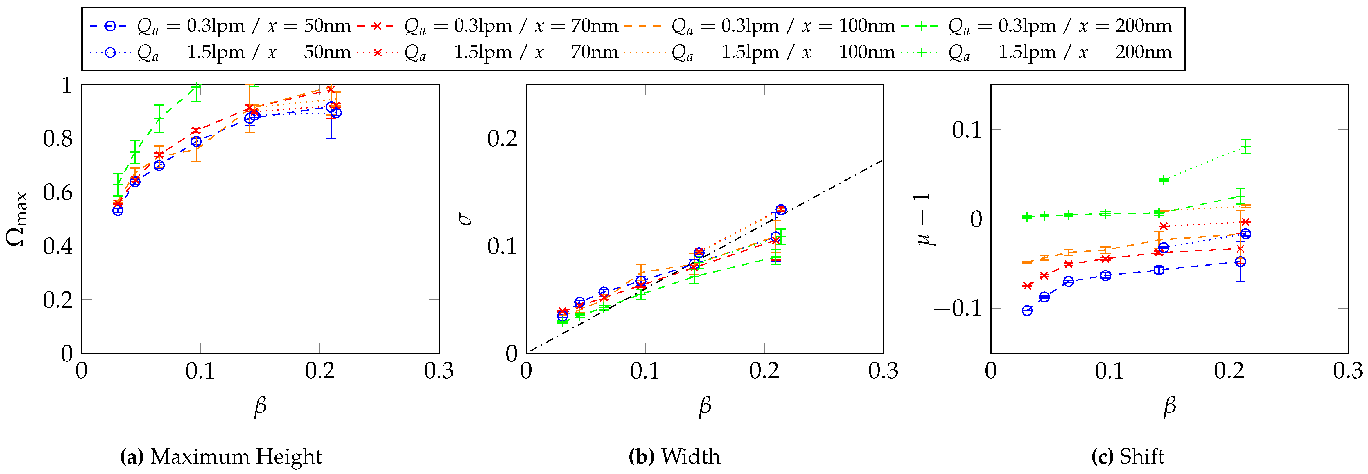
Figure A7.
Measured transfer function parameters of the the DMA combination 3-2, with 95% confidence interval derived out of three samples.
Figure A7.
Measured transfer function parameters of the the DMA combination 3-2, with 95% confidence interval derived out of three samples.
Appendix C. Two-Dimensional Property Distribution for Agglomerated Silver Particles Treated at Different Sintering Temperatures
Figure A8.
Measurement results for silver particles at a sintering temperature of 250 °C.
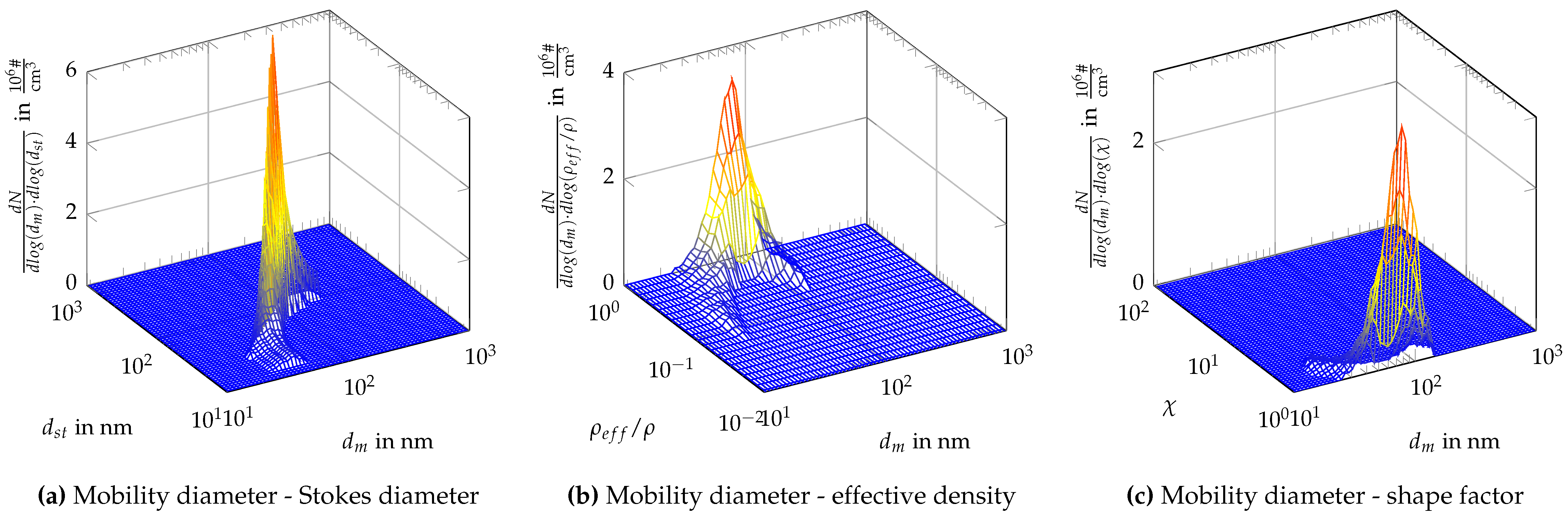
Figure A9.
Measurement results for silver particles at a sintering temperature of 100 °C.
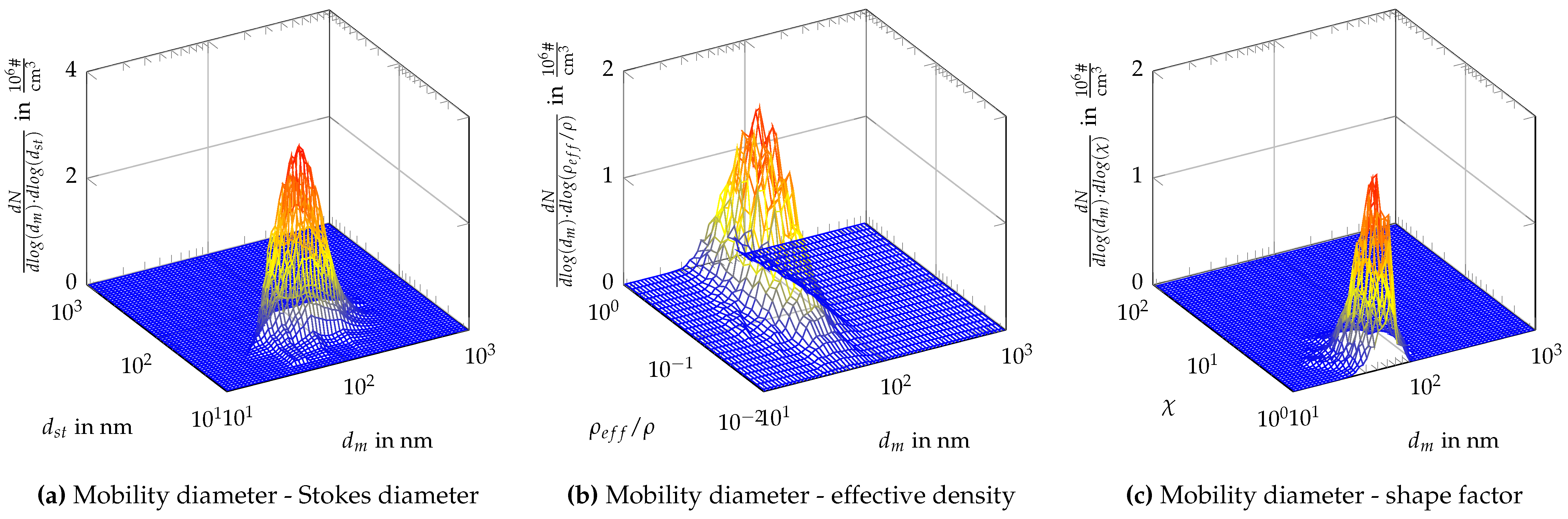
Figure A10.
Measurement results for silver particles at a sintering temperature of 60 °C.
References
- Tavakoli, F.; Olfert, J.S. Determination of particle mass, effective density, mass–mobility exponent, and dynamic shape factor using an aerodynamic aerosol classifier and a differential mobility analyzer in tandem. Journal of Aerosol Science 2014, 75, 35–42. [Google Scholar] [CrossRef]
- Knutson, E.O.; Whitby, K.T. Aerosol classification by electric mobility: apparatus, theory, and applications. Journal of Aerosol Science 1975, 6, 443–451. [Google Scholar] [CrossRef]
- Park, K.; Dutcher, D.; Emery, M.; Pagels, J.; Sakurai, H.; Scheckman, J.; Qian, S.; Stolzenburg, M.R.; Wang, X.; Yang, J.; et al. Tandem Measurements of Aerosol Properties—A Review of Mobility Techniques with Extensions. Aerosol Science and Technology 2008, 42, 801–816. [Google Scholar] [CrossRef]
- Slowik, J.G.; Stainken, K.; Davidovits, P.; Williams, L.R.; Jayne, J.T.; Kolb, C.E.; Worsnop, D.R.; Rudich, Y.; DeCarlo, P.F.; Jimenez, J.L. Particle Morphology and Density Characterization by Combined Mobility and Aerodynamic Diameter Measurements. Part 2: Application to Combustion-Generated Soot Aerosols as a Function of Fuel Equivalence Ratio. Aerosol Science and Technology 2004, 38, 1206–1222. [Google Scholar] [CrossRef]
- Tavakoli, F.; Olfert, J.S. An Instrument for the Classification of Aerosols by Particle Relaxation Time: Theoretical Models of the Aerodynamic Aerosol Classifier. Aerosol Science and Technology 2013, 47, 916–926. [Google Scholar] [CrossRef]
- Stolzenburg, M.R. An Ultrafine Aerosol Size Distribution System. Disseratation, University of Minnesota, Minnesota, 1988.
- Rüther, T.N.; Rasche, D.B.; Schmid, H.J. The Centrifugal Differential Mobility Analyser – A new device for determination of two-dimensional property distributions. [CrossRef]
- Li, W.; Li, L.; Chen, D.R. Technical Note: A New Deconvolution Scheme for the Retrieval of True DMA Transfer Function from Tandem DMA Data. Aerosol Science and Technology 2006, 40, 1052–1057. [Google Scholar] [CrossRef]
- DeCarlo, P.F.; Slowik, J.G.; Worsnop, D.R.; Davidovits, P.; Jimenez, J.L. Particle Morphology and Density Characterization by Combined Mobility and Aerodynamic Diameter Measurements. Part 1: Theory. Aerosol Science and Technology 2004, 38, 1185–1205. [Google Scholar] [CrossRef]
Figure 1.
Cross-section of the CDMA prototype [7]
Figure 1.
Cross-section of the CDMA prototype [7]
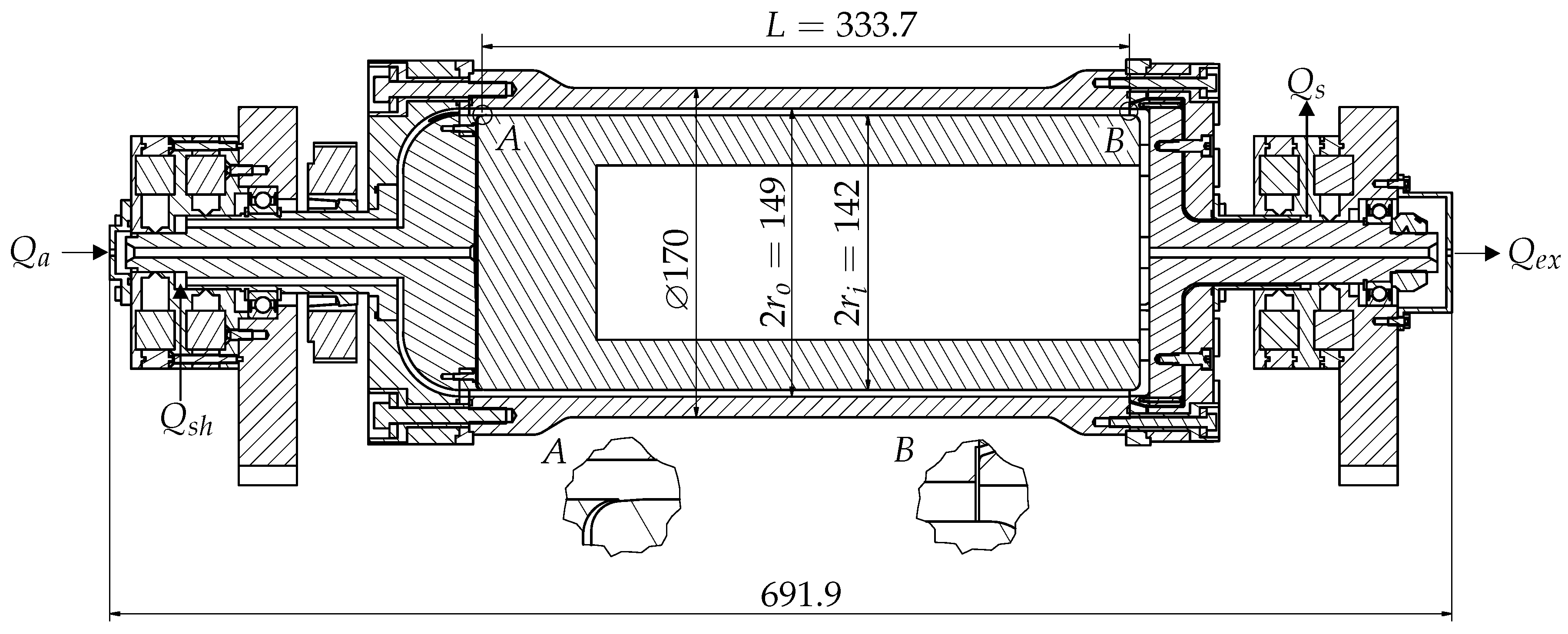
Figure 2.
An eighth of the flow domain used for the calculations including the boundary conditions.
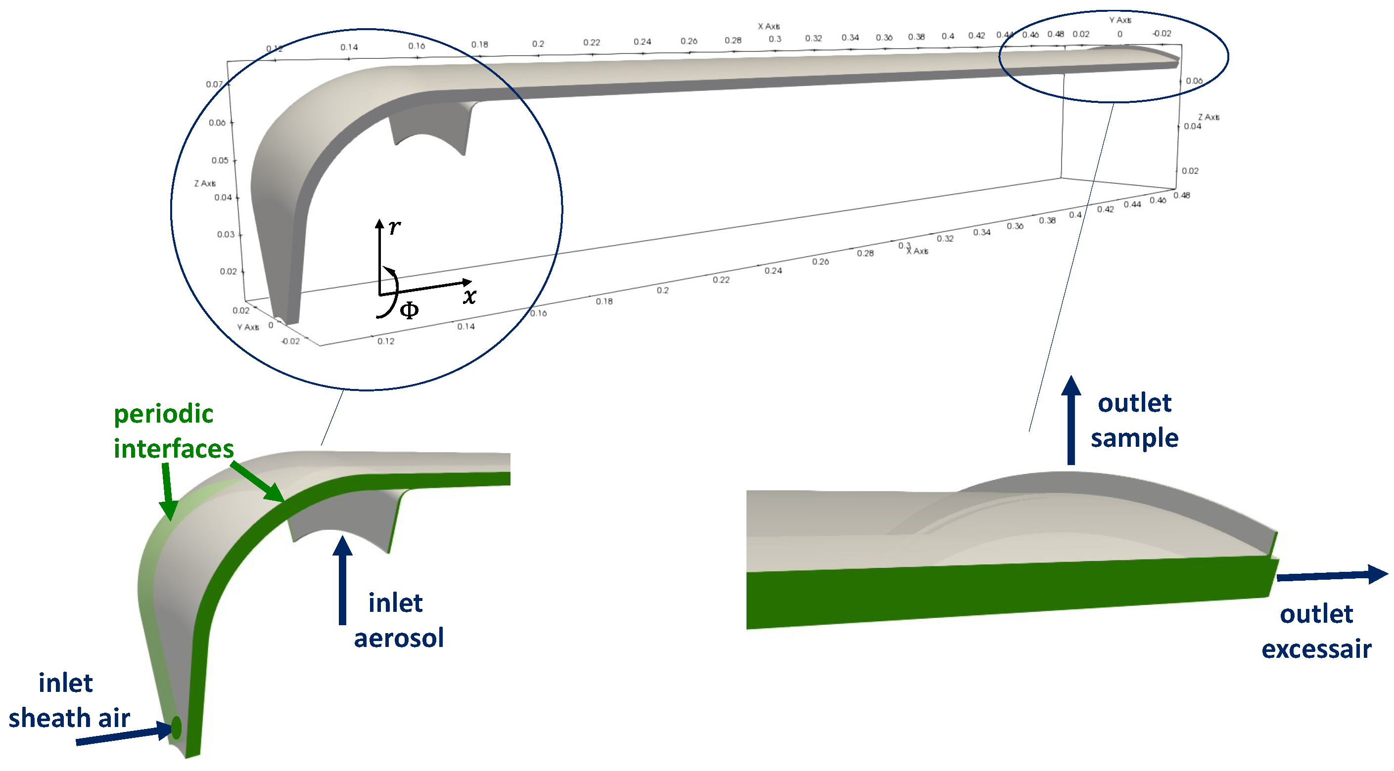
Figure 3.
Cross-sections of the axial flow at different axial coordinates in the proximity of the aerosol inlet. White lines within the displayed planes represent the sources for the plots in Figure 4.
Figure 3.
Cross-sections of the axial flow at different axial coordinates in the proximity of the aerosol inlet. White lines within the displayed planes represent the sources for the plots in Figure 4.
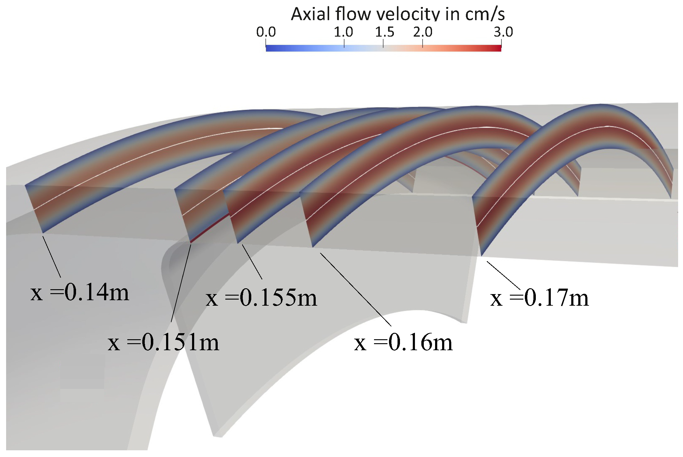
Figure 4.
Plots of the axial velocities for 0 RPM at the middle of the gap () at different axial coordinates. The rotational coordinate represents the angle relative to the middle plane (c.f. Figure A1). Source of the plots are the white lines displayed in Figure 3.
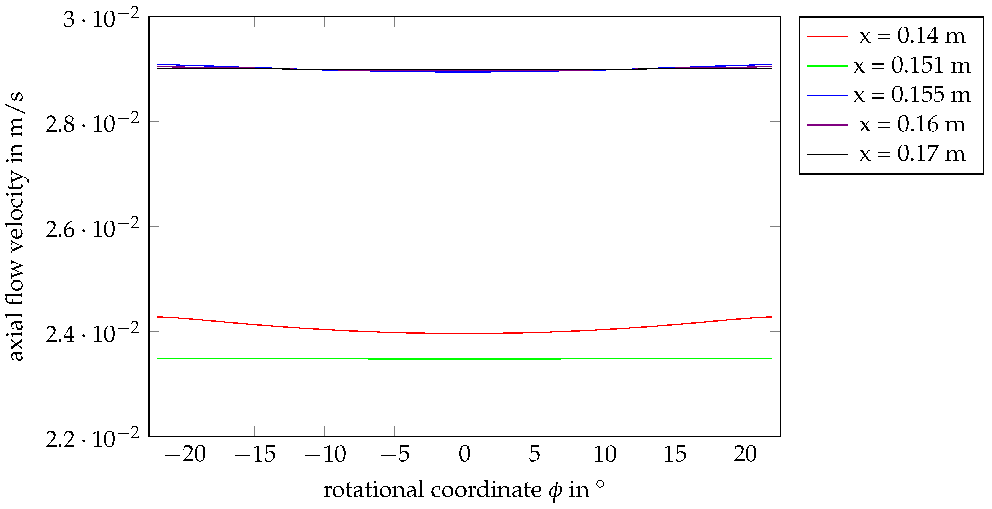
Figure 5.
Streamlines along the middle plane of the flow domain, for 0.3 lpm and 1.5 lpm. The bottom set of streamlines is starting from the aerosol inlet while the upper one ends at the sample outlet.
Figure 5.
Streamlines along the middle plane of the flow domain, for 0.3 lpm and 1.5 lpm. The bottom set of streamlines is starting from the aerosol inlet while the upper one ends at the sample outlet.
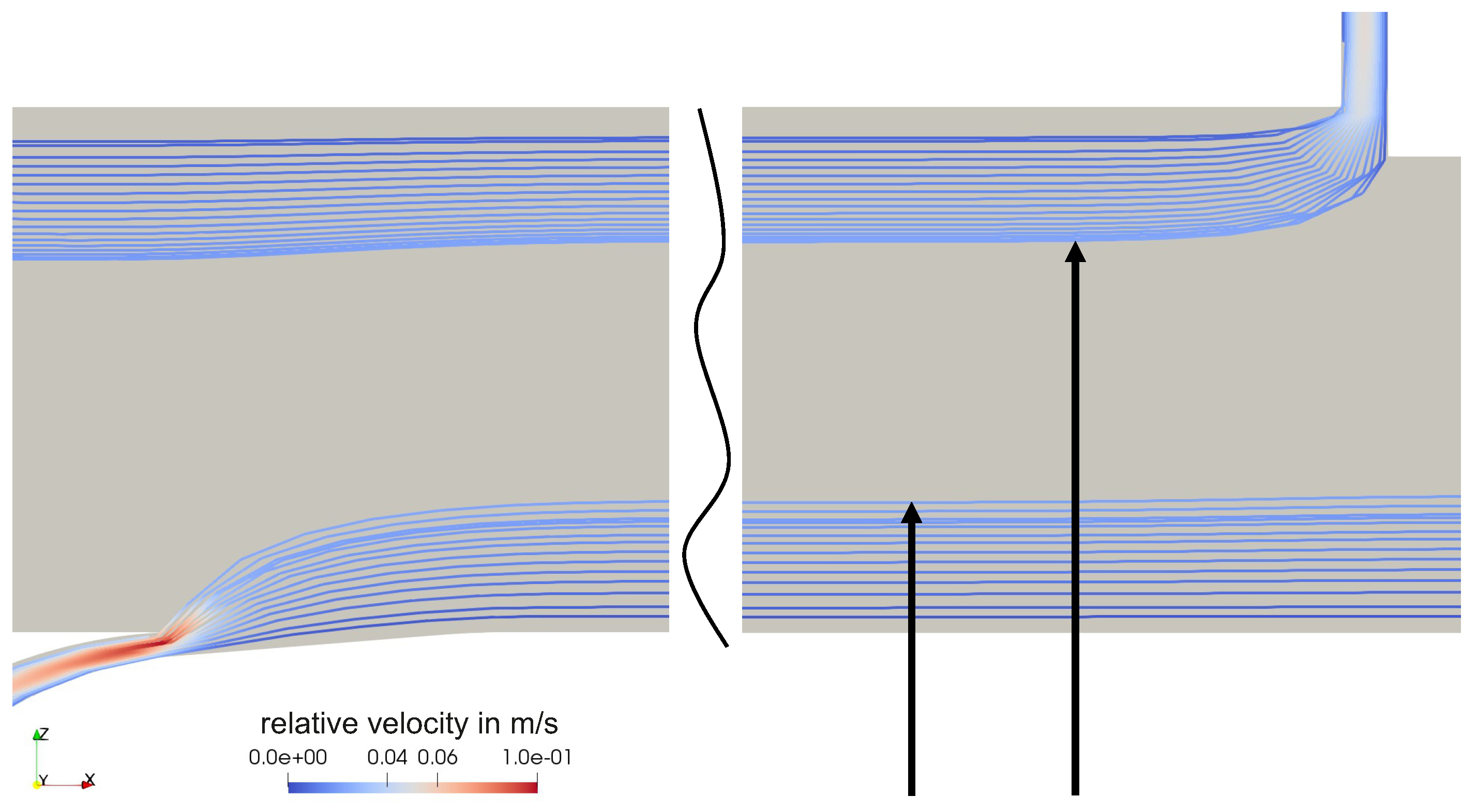
Figure 6.
The effective cross-section for the axial flow reduces with increasing rotational speed. This might be the case as the air builds up at the outer wall due to centrifugal forces.
Figure 6.
The effective cross-section for the axial flow reduces with increasing rotational speed. This might be the case as the air builds up at the outer wall due to centrifugal forces.
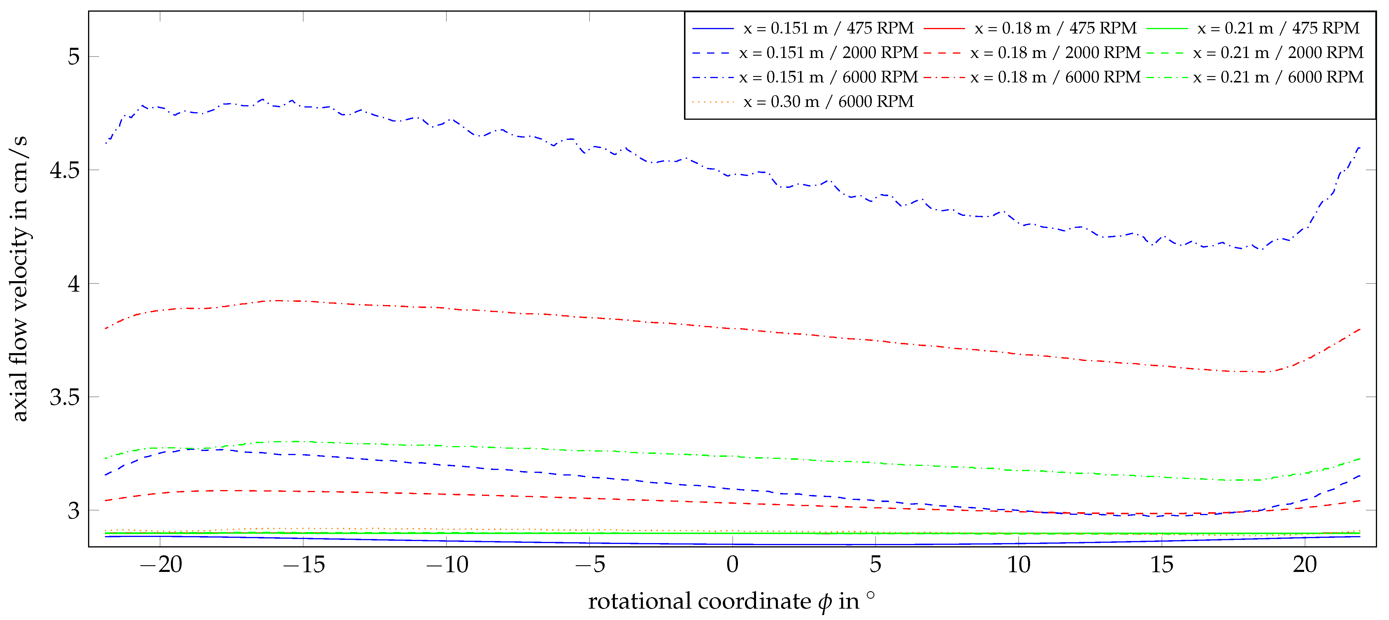
Figure 7.
With increasing rotation number, it takes longer for the flow do adopt its direction to the rotational speed when flowing through the transfer domain.
Figure 7.
With increasing rotation number, it takes longer for the flow do adopt its direction to the rotational speed when flowing through the transfer domain.
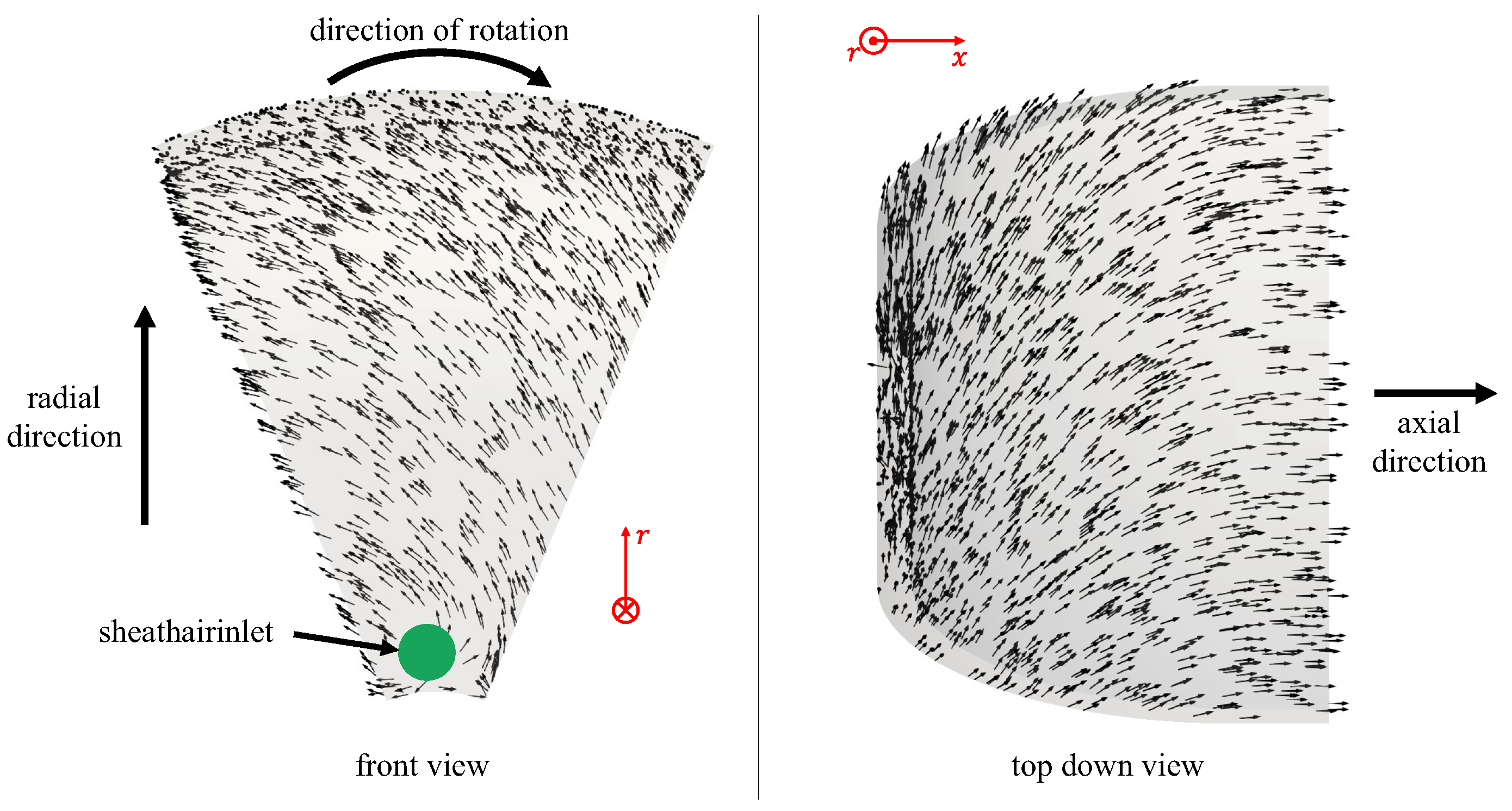
Figure 8.
The effective cross-section for the axial flow reduces with increasing rotational speed. This might be the case as the air builds up at the outer wall due to centrifugal forces.
Figure 8.
The effective cross-section for the axial flow reduces with increasing rotational speed. This might be the case as the air builds up at the outer wall due to centrifugal forces.
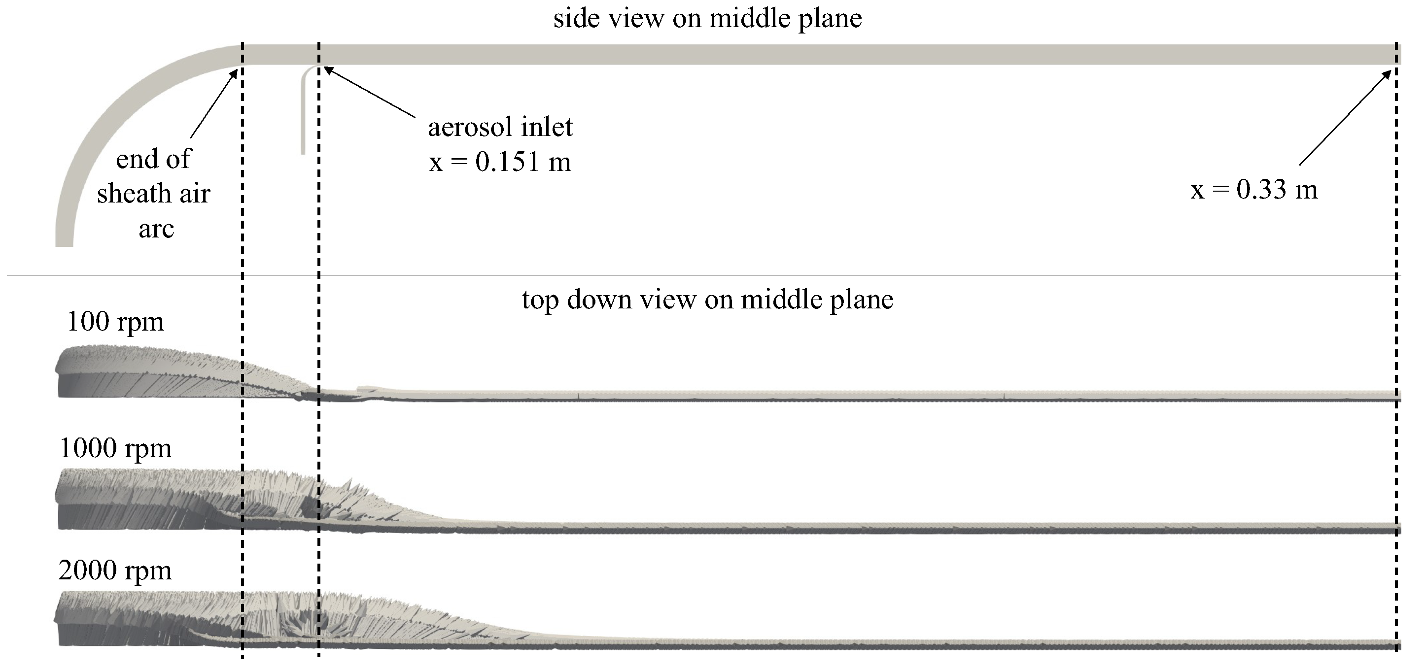
Figure 9.
The beginning of an exemplary trajectory calculated by the algorithm. In this figure, the available data points for flow values are displayed in black. The actual particle trajectory is plotted in green, while the data points, that have been accessed by the algorithm are plotted in red.
Figure 9.
The beginning of an exemplary trajectory calculated by the algorithm. In this figure, the available data points for flow values are displayed in black. The actual particle trajectory is plotted in green, while the data points, that have been accessed by the algorithm are plotted in red.
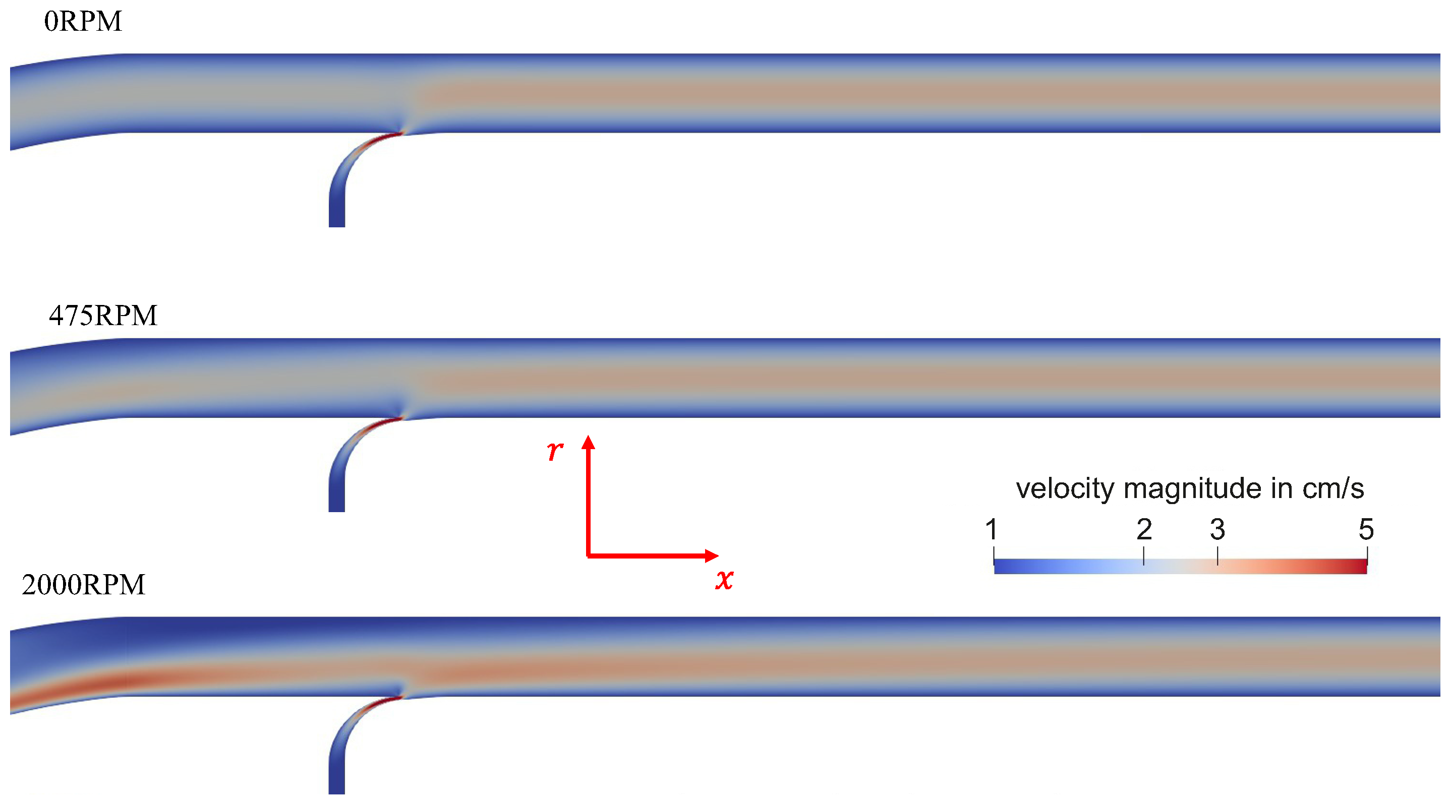
Figure 10.
Trajectories labeled in green are successfully sampled as they end within the axial coordinates of the sample outlet. The trajectories labeled in red are not classified as their last axial coordinate is larger than the axial position of the outlet.
Figure 10.
Trajectories labeled in green are successfully sampled as they end within the axial coordinates of the sample outlet. The trajectories labeled in red are not classified as their last axial coordinate is larger than the axial position of the outlet.
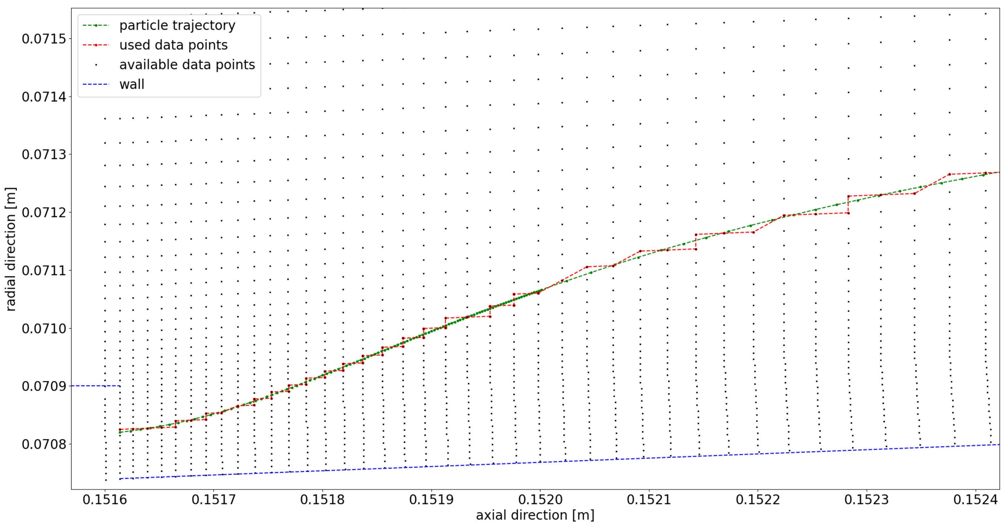
Figure 11.
Ideal two-dimensional transfer function with and . The dashed red lines represent transfer functions for and . The solid red line represents the transfer function of one pair of operating parameters if only spherical particles were present.
Figure 11.
Ideal two-dimensional transfer function with and . The dashed red lines represent transfer functions for and . The solid red line represents the transfer function of one pair of operating parameters if only spherical particles were present.
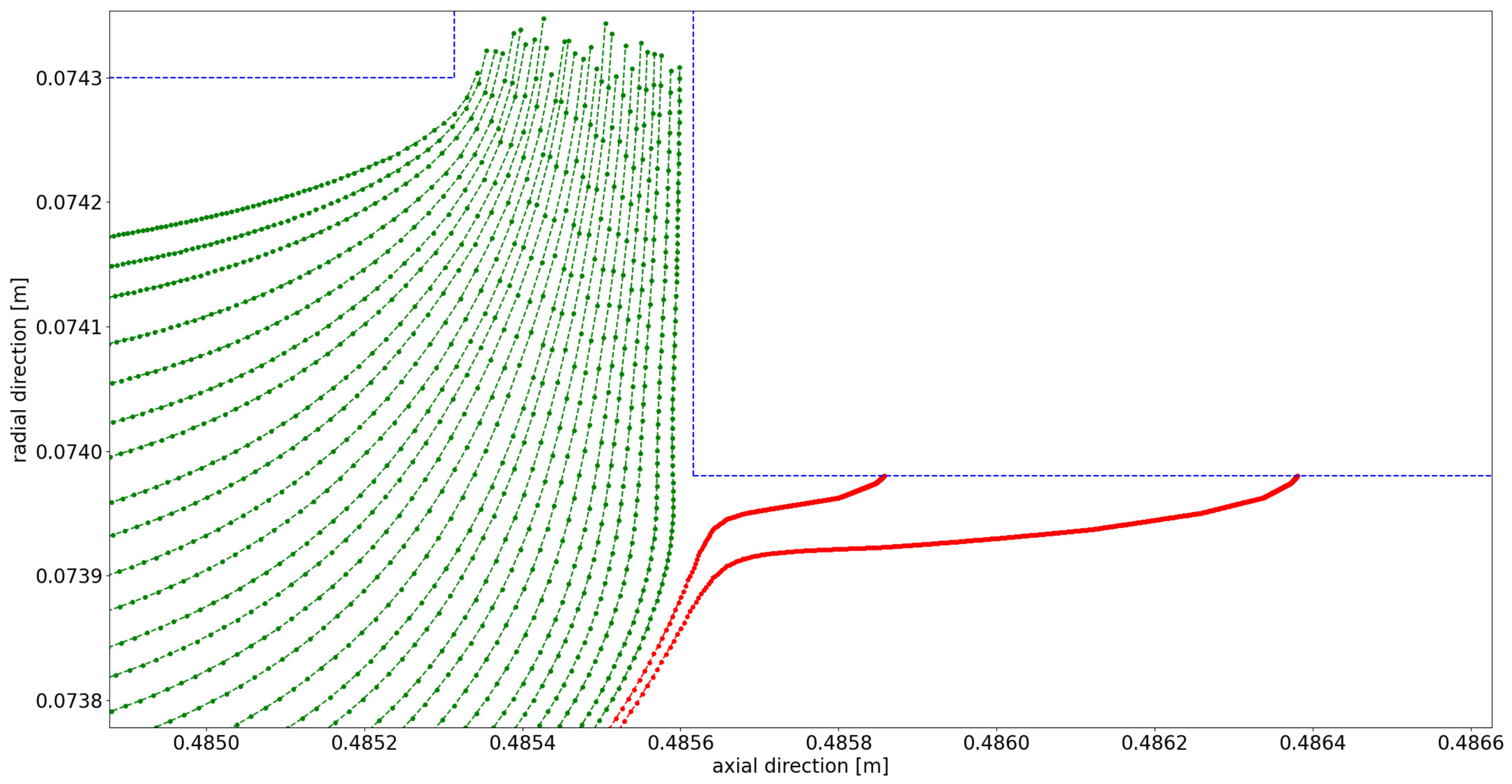
Figure 12.
Schematic of the entire experimental setup: Test aerosol production with two tubefurnaces (Nabertherm) and an agglomeration tube and the consecutive setup consisting of a classifier (TSI 3080) with a DMA (TSI 3081), CDMA and CPC (TSI 3775) for the measurement of a transfer function [7].
Figure 12.
Schematic of the entire experimental setup: Test aerosol production with two tubefurnaces (Nabertherm) and an agglomeration tube and the consecutive setup consisting of a classifier (TSI 3080) with a DMA (TSI 3081), CDMA and CPC (TSI 3775) for the measurement of a transfer function [7].
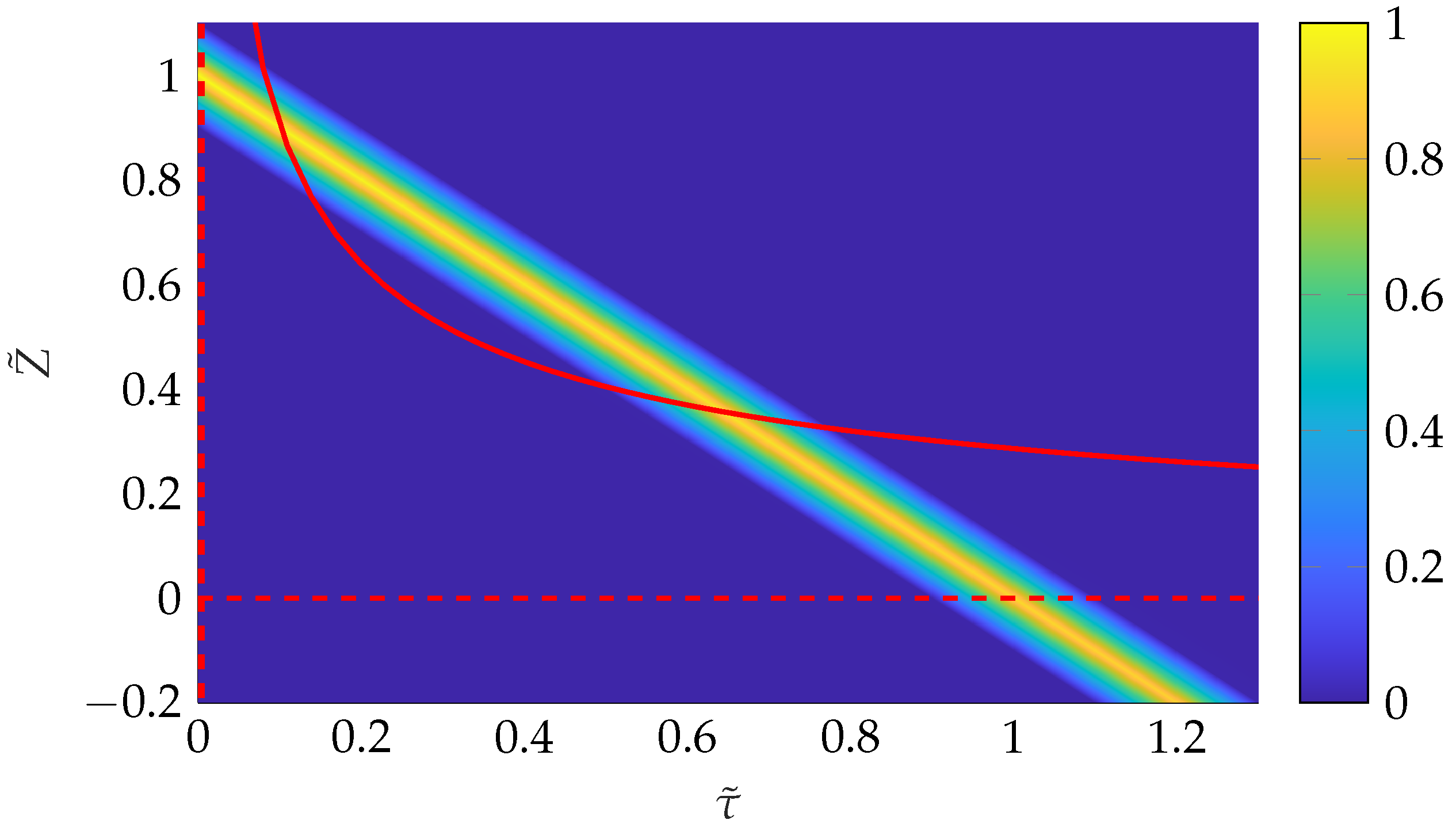
Figure 13.
Schematic of the experimental setup for investigation of the two-dimensional distribution at different sintering stages: Test aerosol production with a tube-furnace (Nabertherm) at (Nabertherm) an agglomeration tube and a sintering tube-furnace (Nabertherm) at , , , , and . Followed by the CDMA (Rüther, forthcoming1) with a classifier (TSI 3080) providing the voltage and sheath air, and a CPC (TSI 3775).
Disclaimer/Publisher’s Note: The statements, opinions and data contained in all publications are solely those of the individual author(s) and contributor(s) and not of MDPI and/or the editor(s). MDPI and/or the editor(s) disclaim responsibility for any injury to people or property resulting from any ideas, methods, instructions or products referred to in the content. |
© 2025 by the authors. Licensee MDPI, Basel, Switzerland. This article is an open access article distributed under the terms and conditions of the Creative Commons Attribution (CC BY) license (http://creativecommons.org/licenses/by/4.0/).
Copyright: This open access article is published under a Creative Commons CC BY 4.0 license, which permit the free download, distribution, and reuse, provided that the author and preprint are cited in any reuse.


