
Submitted:
16 January 2025
Posted:
16 January 2025
You are already at the latest version
Abstract
This work investigates the potential of a sorption-based thermal energy storage (TES) system for enhancing the integration of renewable energy and waste heat recovery in key sectors—industry, transport, and buildings. Sorption-based TES systems, which utilize reversible sorbent-sorbate reactions to store and release thermal energy, offer long-term storage capabilities with minimal losses. A thermodynamic model, supported by experimental data, evaluates the efficiency of various working pairs under different operating conditions. Key findings demonstrate that water-based solutions (e.g., zeolite and silica gel composites) perform well for residential and transport applications, while methanol-based solutions, such as LiCl-silica/methanol, maintain higher efficiency in industrial contexts. Short-term storage shows higher energy efficiencies compared to long-term applications, and the choice of working pairs significantly influences performance. Industrial applications face unique challenges due to extreme operating conditions, limiting the viable solutions to water-based working pairs. This research highlights the capability of sorption-based TES systems to reduce greenhouse gas emissions, improve energy efficiency, and facilitate a transition to sustainable energy practices. The findings contribute to developing cost-effective and reliable solutions for energy storage and renewable integration in various applications.
Keywords:
sorption-based thermal energy storage
; renewable energy integration
; waste heat recovery
; thermodynamic efficiency analysis
; adsorption
1. Introduction
Although 2020 emissions were lower than in 2019 as a result of the COVID-19 crisis and subsequent countermeasures [1], greenhouse gas (GHG) concentrations in the atmosphere continue to rise, with the immediate reduction in emissions predicted to have a minor long-term influence on climate change.
In 2023, global GHG emissions increased by 1.3% compared to 2022, reaching a new high of 57.1 GtCO2e. The annual percentage increase is higher than the average value recorded in the last decade (2010-2019), equal to 0.8%. Total GHG emissions are dominated by fossil carbon dioxide (CO2) emissions (from fossil fuels and carbonates). According to preliminary estimates, fossil CO2 emissions in 2023 set a new high of 38.8 GtCO2 [2]. In contrast, global GHG emissions in 2030 need to be approximately 25% and 55% lower than in 2017 to put the world on a least-cost pathway to limiting global warming to 2 °C and 1.5 °C, respectively [3].
Global CO2 emissions are above the targets set by the agreements on Mitigation of Climate Change and the national governments. The major reason is that although energy efficiency considerably improved and renewables have been installed at a large scale, this was overcompensated by economic growth resulting in an increase of emissions.
One of the combinations that have aroused the most interest is the exploitation of solar heat by using thermal energy storage (TES), which has been widely studied and simulated in different research papers. Zhu et al. [6], for instance, investigated the performance of sensible-type thermocline TES for civil and industrial scenarios using a two-dimensional flow and heat transfer model of a single-tank TES system providing useful findings for the design of heat storage for solar integration in industry. In Ref. [7] the authors reviewed the integration strategies of solar heat in industrial processes by studying heating systems, solar collectors and thermal storage. It was found that for the food, beverage, and agriculture sectors, 51% of solar process heat integration occurs at the supply level and 27.3% at the process level. Biencinto et al. [8] proposed an innovative thermal storage system to support the contribution of the solar field to the industrial heat demand. They simulated a TES based on the latent heat of the solid-solid transition of pentaglycerine by means of TRNSYS software. Annual simulations have been performed using meteorological data from Graz (Austria) and Plataforma Solar de Almería (Spain). Results showed that annual heat demand covered with solar energy could be increased by 7% in Graz and by 12% in Almeria by using 3 h of latent heat storage.
In particular, the study in this paper introduces one of the most promising innovative heat storage technology, the sorption-based TES, for application in different fields.
However, a few studies available in the literature investigated the potential of such a class of systems. Years ago, Kronauer et al. [9] presented a mobile TES system working with Zeolite in an open cycle that can utilize industrial waste heat to easily transfer large amounts of thermal energy where a stable connection through a pipe is not possible. The storage “cartridge” contains 14 tons of Zeolite with a storage capacity of 2.3 MWh (@ 60°C): the authors demonstrated that is possible to reduce energy cost down to 73 €/MWh considering a small-scale mass production.
Such technology can effectively increase the exploitation of renewables (i.e., solar thermal energy to cover heat demand) with the scope to set or increase renewable energy integration and flexibility in selected and suitable industrial processes. Moreover, the long-term heat storage as well as the combined cold & heat storage can be realized by sorption-based TES. Recently, some zeolite composite materials have been applied to the long sorption heat storage, demonstrating a heat storage density of up to 0.3 kWh/kg [10,11]. However, such materials are still under development, not commercially available and expensive.
The present study aims to evaluate the potential of advanced energy storage systems (based on cheap and widely available sorption materials) for renewables and waste heat integration. The analysis is based on the calculation of the storage efficiency of the sorption-based TES through a thermodynamic model based on experimental measurements. In particular, the thermodynamic model allows the identification of the best working pairs through a comparative analysis between different options. The three fields of application that contribute most to global CO2 emissions have been taken into consideration: industry, transport and buildings [12]. The overall impact is to enhance primary energy savings, leading to reduced greenhouse gas (GHG) emissions and fossil fuel utilization, thus contributing to energy security and supply, reduction in CO2 and pollutant emissions and reaching reliable and cost-effective solutions.
2. Concept Description
The studied system is based on a sorption storage technology, which relies on the reversible reaction, associated with a high amount of thermal energy, occurring between a sorbent and a sorbate. Such a process is limited by the slow reaction kinetics, because of the large amount of heat associated as well as the heat and mass transfer diffusion resistance within the material. However, this feature is extremely useful in an industrial-type application, since it allows the reaction to be safely controlled and the discharge power to be regulated precisely.
In the proposed concept, heat from a renewable energy source (e.g., solar heat) is employed to drive a desorption process, which means that incoming heat is stored in the form of adsorption potential energy. Moreover, the heat is stored without any loss until the refrigerant fluid (adsorbate) is kept separated from the adsorbent enabling the long-term storage of the renewable energy.
Generally, there are two system configurations for adsorption TES: closed and open cycle [13]. The studied heat storage system belongs to the closed-cycle sorption storage category.
Figure 1 reports the working phases of closed adsorption. During the charging phase, the adsorber, in which the adsorbent material is saturated with adsorbate, is regenerated by exploiting heat, e.g., heat coming from the solar field. The desorbed vapour is then condensed in the condenser, and the heat of condensation, Qcond, is either dissipated in the ambient or delivered to a proper load if the temperature level is adequate. Once the charging process is completed, and the adsorbent material is dry, the connection between the condenser and adsorber is closed. In this condition, the system can keep the stored energy for an indefinite time since the thermal energy is stored as adsorption potential between adsorbate and adsorbent material. To recover the stored thermal energy the connection between the liquid adsorbate reservoir, which in this phase acts as an evaporator, and the adsorber is again opened. During this discharging phase, the adsorbate is evaporated adsorbing heat from the ambient, Qevap, or providing a cooling useful effect to a specific user. Then, the vapour fluxes to the adsorber and, since the adsorption process is exothermic, the heat stored is released to the load. It is self-evident that in this heat storage system the adsorbate is continuously condensed/evaporated in a closed device without any mass exchange with the ambient; this feature ensures the proper functioning of the adsorption TES system also in dry climates.
Figure 2 and Figure 3 depict an example of the proposed concept integrated into an industrial context. It consists of the coupling of a Concentrating Solar Field (CSF) with advanced sorption storage (which uses water as refrigerant). As previously explained, the phase changer acts alternatively as an evaporator or condenser during the different phases. Indeed, during the operation of the system, two distinct phases can be distinguished:
- Charging phase: the heat provided by the solar field, at the maximum temperature level in the system, feeds the sorption storage system and the high-temperature (HT) user into the industrial process. In the sorption storage system, the adsorbent material is heated and desorbed until it reaches the maximum temperature. The refrigerant desorbed (water) is condensed in the phase changer and the heat of condensation is released in the ambient through an air/water cooler.
- Discharging phase: when the solar heat is not available anymore, the system operates as depicted in Figure 3. The heat absorbed by the HT user cools down the storage. When the reactor is cooled until its pressure drops below the phase changer pressure, the adsorbent material begins adsorbing refrigerant vapour from the phase changer (acting as an evaporator) and releases the stored heat. The needed heat of evaporation can be provided at Low Temperature (LT) by an industrial process that needs to be cooled (I.C.E., air compressors, mould cooling, etc.). The sorption storage system is preferably used in this way because, by actively cooling processes during discharge, the heat of evaporation is a “useful heat” too. This leads to a heat storage efficiency > 1, which means that the storage system is actively saving additional energy. If there is no process available to be cooled, the heat of evaporation may be absorbed from the air. In this case, the storage efficiency is < 1 and the advantage compared to common sensible pressurised water storage is a much higher storage density and lower thermal losses.
It is worth spending some further explanation to better clarify this point. In TES systems, the energy storage efficiency is defined as the ratio of useful energy output to the energy input (see next section). For sorption-based TES systems, the efficiency can exceed 1 in specific configurations and operating conditions due to the active cooling effect and energy recovery mechanisms. Indeed, during the discharging phase, the evaporator absorbs heat from a low-temperature source (e.g., ambient air or a cooling process). This heat, along with the stored thermal energy, is delivered to the loads (at different temperatures). The additional heat absorbed from the surroundings increases the total useful energy output, allowing the efficiency to surpass 1. This phenomenon is similar to the performance of heat pumps, where low-grade heat is effectively upgraded for useful applications.
Moreover, in a well-designed TES system, heat released during condensation in the condenser can be recovered and reused, either for preheating or other low-temperature applications. Similarly, the adsorption process releases significant exothermic heat, which can also be utilized. These mechanisms allow for enhanced utilization of the input energy.
By leveraging these effects, sorption-based TES systems can achieve efficiencies greater than 1, effectively providing more useful energy than direct input energy, thus maximizing energy savings and reducing waste.
3. Estimation of Storage Performance
The estimation of the performance for a preliminary evaluation of the potentialities of the proposed system has been carried out through a simplified and robust mathematical model. The model used for the study has the objective of describing a thermodynamic cycle of a storage unit, usually represented in a Clapeyron diagram (see Figure 4), to determine the corresponding efficiency and allow the comparison of different adsorbent materials.
As already introduced in the previous sections, the basic storage sorption cycle consists of four phases grouped in the two typical stages of a storage system: the charging phase consisting of isosteric heating (Phase 1), isobaric desorption (Phase 2), the discharging phase consisting of an isosteric cooling (Phase 3), and isobaric adsorption (Phase 4).
To facilitate the study, the following assumptions have been made:
- the temperatures of the evaporator and condenser are constant and are indicated as Tev and Tcond;
- the minimum and maximum temperatures of the cycle are known: Tmin ≡ T1 and Tmax ≡ T3;
Once Tev and Tcond are known, the pressure of the evaporator and condenser (Pev and Pcond) can be determined. The equilibrium of adsorbent and adsorbate can be described by several models reported in literature (e.g., Freundlich’s model, Dubinin-Radushkevich, etc.), however in this study, the Clausius-Clapeyron phenomenological law has been implemented [14], as it revealed to be adequate to describe the adsorbent/adsorbate equilibrium for the more promising working pairs identified for application in a storage unit.
An iterative procedure has been used to determine the uptake: the maximum and minimum uptake values, which correspond to the two isosteric conditions of the thermodynamic cycle, are established based on the thermal-pressure conditions. The Newton-Raphson method is used to calculate the uptake from the non-linear equation describing the equilibrium between adsorbent and adsorbate:
where A(w) and B(w) are third-order polynomials, calculated through coefficients determined experimentally and which depend on the working pair:
The temperatures T2 and T4, corresponding respectively to the start of Phase 2 and start of Phase 4 of the cycle, can be determined as a function of the operating conditions:
The mentioned calculations allow the determination of the three values (pressure, temperature and uptake) that allow the identification of the four points that define the thermodynamic cycle of the storage system.
Knowledge of these values allows the calculation of storage efficiency.
3.1. Determination of the Storage Energy Efficiency
Storage efficiency is a parameter calculated to compare different TES systems. In its most classical definition, storage energy efficiency can be described as the ratio between the useful energy and the input energy of the storage system [15]:
In this paper, the storage efficiency is calculated considering the best case, in which it is possible to recover both the heat exiting the condenser (for heating operations) and the heat required by the evaporator (for cooling operations). The efficiency evaluation refers to two fundamental conditions. The first one is for short-term storage (ideally with zero storage time); the efficiency calculation is described by the following formula:
The second condition represents long-term (ideally infinite) storage. In this case, the stored sensible heat related to the four phases of the thermodynamic cycle is totally dissipated. The useful heat is therefore reduced to the heat associated with the condenser and the evaporator, in addition to the adsorption heat (Qh):
The calculation of heat flows follows the indications given in Ref. [16]. The heat of the condenser and evaporator can be calculated as a function of temperature:
is the latent heat of the refrigerant at temperature T, relative to the amount of refrigerant desorbed:
Qsv refers to the sensible heat released (or supplied) to cool (or heat) the vapour until it reaches the condensation (or adsorption) temperature:
where represent the specific heat of the refrigerant vapour and the temperature Tavg is defined as:
The term Qi, for i = 1 – 4, represents the total heat associated with each of the four phases that make up the storage cycle, and is made up of three contributions:
with β = 0 for the isosteric heating and cooling phases (i = 1,3) and β = 0 for the isobaric desorption and adsorption phases (i = 2,4); γ is equal to zero for i = 1,2,3 while for Phase 4 (isobaric adsorption) it is γ = 1.
Qs,i represents the sensible heat associated with heating or cooling the adsorbent bed. It consists of a term relating to the adsorbent rich in adsorbed refrigerant and a term relating to the metal mass present in the bed (ϕ represents the metal/adsorbent mass ratio):
where w(T) is equal to wmax for i = 1 and it is equal to wmin for i = 3, while for i = 2,4 an average value between wmin and wmax is considered.
The equivalent specific heat is a function of the uptake and the temperature and can be calculated as:
where C(w) and D(w) are second order polynomials described by experimental coefficients specific for each working pair:
The experimental coefficients ci and di are not available for all the considered working pairs. In these cases the equivalent specific heat can be calculated as a linear combination between the specific heat of the dry adsorbent and the refrigerant [17]:
where the specific heat of the adsorbed refrigerant is considered equal to that of the non-adsorbed refrigerant in the liquid state, as indicated in Ref. [18].
Qh represents the heat of desorption supplied or the heat of adsorption released and is calculated using the following equation:
where ΔH is the adsorption/desorption enthalpy, calculated as:
where B is the experimental coefficient described previously (see Equation (2b)), R is the universal gas constant and Mv is the molecular mass of the adsorbate.
4. Simulation Results
The formulas described in the previous section allow us to build a thermodynamic model used to evaluate the energy efficiency of the TES system. The model offers the possibility of carrying out a comparative study between various working pairs used in different working conditions. The working conditions considered refer to three different possible applications of the TES system: buildings, transport and industry. Each application is characterized by different boundary conditions expressed in terms of different temperature levels, reported in Table 1.
Several working pairs were selected, consisting of different adsorbent materials and three refrigerants: methanol, ethanol and water. Not all working pairs can be used for the three applications considered. In fact, for some working pairs the boundary conditions identify uptake values outside the valid range. This happens especially for industrial applications, where the working conditions are extreme for many solutions. Table 2 shows the working pairs considered acceptable for each application (for practical reasons, each pair is associated with an identification code).
The next paragraphs summarize the main results obtained for the three selected applications. For each of these, the thermodynamic model is used to simulate two operating conditions:
- Short-therm storage (t = 0);
- Long-term storage (t = ∞);
As described by the formulas presented in the previous section, the amount of energy stored and made available by the TES system also depends on the amount of metal mass present in the adsorbent bed. To take into account this dependence, the following parameter, the metal/adsorbent mass ratio, is introduced:
For each case considered, the storage efficiency is calculated for different values assumed by ϕ (i.e., η0 for ϕ = 0, η1 for ϕ = 0.5, η2 for ϕ = 1, η3 for ϕ = 2 and η4 for ϕ = 3).
4.1. Determination of Experimental Coefficients
The calculation of the energy efficiency of the storage system requires the identification of the values assumed by the experimental coefficients (ai, bi, ci, di) that appear in the formulas provided above. The first two coefficients (ai and bi, with i = 0−3) are necessary for the calculation of A(w) (see Equation (2a)) and B(w) (Equation (2b)), which define the adsorbent-adsorbate equilibrium equation (Equation (1)), while ci and di (with i = 0-2) are used to calculate the equivalent specific heat of the working pair, as shown in Equations (14), (15a) and (15b). These coefficients are identified experimentally by calorimetric technique described in Ref. [17]. The experimental analyses were conducted on a thermo-gravimetric apparatus installed in the CNR-ITAE laboratories. This apparatus allows to replicate the main phases of the thermodynamic cycle, measuring the equilibrium curves and the heat flows. Table 3 and Table 4 show the coefficient values that were obtained for each working pair considered.
As anticipated in the previous section, the coefficients ci and di are available only for some working pairs (unlike ai and bi, whose values are available for all solutions). For pairs whose coefficients are not available, the equivalent specific heat is calculated as described by the Equation (16) reported previously.
4.2. Buildings
Table 5 shows the values that define the thermodynamic sorption cycle for each working pair used in the residential application.
Figure 5 shows the energy efficiencies of short-term storage, as the mass of metal present in the adsorbent bed varies. In general, the most promising values are associated with the use of water as a refrigerant; in particular the most promising working pairs are the zeolite DDZ70 UOP/water (CM13) and the composite CaCl2-silica/water (CM09) solutions. The first one offers the best performance in the absence of metal mass (η0 = 3.46), but undergoes a strong reduction as ϕ increases. Methanol or ethanol based solutions generally show lower efficiencies, except for the composite LiCl-silica/methanol solution (CM04), which is characterized by a rather limited reduction in performance as the metal mass increases: for ϕ = 3 this is the working pair with the best performance, with a storage energy efficiency of 2.65. Figure 6 instead shows the efficiency values in the case of long-term storage (ideally infinite). The zeolite DDZ70 UOP/water solution (CM13) is still the best choice for ϕ = 0, but has again a very critical reduction in the presence of metal mass. The LiCl-silica/methanol mixture (CM04) appears to be even more promising than in the case of short-term storage: it is the working pair with the highest performance for ϕ > 1. Despite presenting good efficiency values, ethanol-based solutions (CM06, CM08) tend to strongly degrade their performance as ϕ and storage time increase.
Figure 7 shows the trend of the storage efficiency of the four most promising working pairs as a function of ϕ, for both cases considered: the water-based working pairs (CM09, CM12, CM13) are more sensitive to the presence of a metal mass in the adsorbent bed, with a significant reduction in performance compared to the methanol-based pairs (e.g., CM04).
4.3. Transport
The points of the thermodynamic cycle characteristic of a possible application of the TES system in the field of mobility are presented in Table 6.
The performances obtained from the simulations on the thermodynamic model are summarized in Figure 8 (for short-term storage) and in Figure 9 (for long-term storage). The conclusions reached for the residential sector remain generally valid. The most interesting difference concerns the Zeolite AQSOA FAM Z02/water mixture (CM12), which already in the previous case appeared to be a promising solution. The application in the field of mobility highlights the characteristic strengths of this working pair: unlike other water-based solutions (e.g., CM09, CM13), the mixture offers performances that resist well to the increase in storage time and ϕ, as clearly shown in Figure 10.
4.4. Industry
In industrial application, high working temperatures and pressures (indicated in Table 7) severely limit the use of many solutions. Among all the working pairs considered, only two (both with water as a refrigerant) are usable: Zeolite SAPO 34 Tianjin/water (CM14) and Silica gel Sorbsil/water (CM17).
Figure 11 and Figure 12 show the energy efficiency of the TES system in the application in industrial environment. In each case considered, the silica gel Sorbsil/water mixture (CM17) represents the optimal choice in terms of performance, although the use of Zeolite SAPO 34 Tianjin as adsorbent (CM14) causes a smaller efficiency loss in the passage from ϕ = 0 to ϕ = 3 (in percentage terms, 16.90% compared to 20.47%); the efficiency loss is more similar in the case of long-term storage (29.08% versus 31.29%), as shown in Figure 13.
5. Conclusions
The development of the thermodynamic model of the adsorption TES system allowed a comparative analysis between different working pairs, through the simulation of three operating conditions. The results obtained have highlighted the high potential in terms of energy efficiency for these advanced thermal storage systems. In particular, the following points summarize the main conclusions reached:
- Water-based solutions generally offer good performance, particularly in the case of zeolite DDZ70 UOP/water and composite CaCl2-silica/water. Despite this, they tend to significantly reduce the efficiency of the system as the metal mass present in the adsorption bed increases (with some exceptions, such as the Zeolite AQSOA FAM Z02/water mixture);
- TES systems using working pairs with methanol as refrigerant show a higher inertia in terms of energy efficiency as the metal mass in the adsorbent bed increases. In particular, the LiCl-silica/methanol solution proves to be a good solution in the case of ϕ higher than 1, especially for long-term storage, being also a little sensitive to the increase in accumulation time;
- The ethanol-based solutions analyzed are not recommended, as their use leads to energy efficiencies that decrease significantly as ϕ and storage time increase;
- The transition from short-term storage (t=0) to long-term storage (t=∞) causes a clear decrease in efficiency. The percentage decrease is particularly high for ethanol-based working pairs, while it is limited when using water and (especially) methanol as refrigerant. In all cases, the reduction is clearly accentuated in the presence of a significant metal mass in the adsorbent bed;
- In the case of application of the TES adsorption system in the residential sector, the working couples consisting of zeolite DDZ70 UOP/water and composite CaCl2-silica/water are the best for low metal/adsorbent mass ratios, while for higher ratios LiCl-silica/methanol shows good results;
- In the case of transport applications, simulations led to similar conclusions to those reached in the residential case. The LiCl-silica/methanol mixture offers even better performance, resulting in many cases the most recommended choice. In the case of long-term storage, the Zeolite AQSOA FAM Z02/water solution arouses great interest, in particular for high values of ϕ;
- For industrial applications, the selection of working pairs is highly critical, due to the critical working conditions, which do not allow the use of many solutions. The only acceptable mixtures among those taken into consideration are the water-based ones, with Zeolite SAPO 34 Tianjin or Silica gel Sorbsil as refrigerant. The latter offers the best performance in terms of energy efficiency, in all the cases considered.
Funding
This study received funding from the European Union - Next-GenerationEU - National Recovery and Resilience Plan (NRRP) – Mission 4, Component 2, Investment N. 1.1, Call PRIN 2022 PNRR D.D. 1409 14-09-2022 – Advanced Thermal Energy Storages On Large Ships (ATOL) – CUP N. B53D23027050001 (Prot. P2022JYLAC).
Conflicts of Interest
The authors declare no conflicts of interest
Abbreviations
The following abbreviations are used in this manuscript:
| GHG | GreenHouse Gas |
| TES | Thermal Energy Storage |
| CSF | Concentrating Solar Field |
| HT | High-Temperature |
| LT | Low-Temperature |
References
- United Nations Environment Programme. Emissions Gap Report 2021: The Heat Is On – A World of Climate Promises Not Yet Delivered. Nairobi, Kenya, 2021. https://www.unep.org/emissions-gap-report-2021.
- United Nations Environment Programme. Emissions Gap Report 2024: No more hot air … please! With a massive gap between rhetoric and reality, countries draft new climate commitments. Nairobi, Kenya, 2024. https://www.unep.org/emissions-gap-report-2024.
- Delbeke, J.; Runge-Metzger, A.; Slingenberg, Y.; Werksman, J. The paris agreement, Towar. a Clim. Eur. Curbing Trend. 2019, 24–45. [Google Scholar] [CrossRef]
- Crespo A.; Barreneche C.; Ibarra M.; Platzer W. Latent thermal energy storage for solar process heat applications at medium-high temperatures – A review, Solar Energy 2019, 192. [CrossRef]
- Koçak B.; Fernandez A.I.; Paksoy H. Review on sensible thermal energy storage for industrial solar applications and sustainability aspects, Solar Energy 2020, 209. [CrossRef]
- Zhu, C.; Zhang, J.; Wang, Y.; Deng, Z.; Shi, P.; Wu, J.; Wu, Z. Study on Thermal Performance of Single-Tank Thermal Energy Storage System with Thermocline in Solar Thermal Utilization. Appl. Sci. 2022, 12, 3908. [Google Scholar] [CrossRef]
- Tasmin, N.; Farjana, S.H.; Hossain, M.R.; Golder, S.; Mahmud, M.A.P. Integration of Solar Process Heat in Industries: A Review. Clean Technol. 2022, 4, 97–131. [Google Scholar] [CrossRef]
- Biencinto, M.; Bayón, R.; González, L.; Christodoulaki, R.; Rojas, E. Integration of a parabolic-trough solar field with solid-solid latent storage in an industrial process with different temperature levels. Applied Thermal Engineering 2021, 184. [Google Scholar] [CrossRef]
- Krönauer, A.; Lävemann, E.; Brückner, S.; Hauer, A. Mobile Sorption Heat Storage in Industrial Waste Heat Recovery. Energy Procedia 2015, 73. [Google Scholar] [CrossRef]
- Hongois, S.; Kuznik, F.; Stevens, P.; Roux, J.-J. Development and characterisation of a new MgSO4−zeolite composite for long-term thermal energy storage. Sol Energy Mater Sol Cell 2011, 95. [Google Scholar] [CrossRef]
- Whiting, G.T.; Grondin, D.; Stosic, D.; Bennici, S.; Auroux, A. Zeolite–MgCl2 composites as potential long-term heat storage materials: influence of zeolite properties on heats of water sorption. Sol Energy Mater Sol Cell 2014, 128, 289–295. [Google Scholar] [CrossRef]
- International Energy Agency, World Energy Outlook 2024, IEA, Paris, France, 2024. https://www.iea.org/reports/world-energy-outlook-2024, (Annex A).
- Vasta, S.; Brancato, V.; La Rosa, D.; Palomba, V.; Restuccia, G.; Sapienza, A.; Frazzica, A. Adsorption heat storage: State-of-the-art and future perspectives. Nanomaterials 2018, 8(7), 522. [Google Scholar] [CrossRef] [PubMed]
- Pons M.; Grenier Ph. A phenomenological adsorption equilibrium law extracted from experimental and theoretical considerations applied to the activated carbon + methanol pair. Carbon, 1986 24 (5), 615–625. [CrossRef]
- Al-Amayreh, M.I.; Alahmer, A. Efficiency enhancement in direct thermal energy storage systems using dual phase change materials and nanoparticle additives. Case Studies in Thermal Engineering 2024, 59. [Google Scholar] [CrossRef]
- Freni, A.; Maggio, G.; Sapienza, A.; Frazzica, A.; Restuccia, G.; Vasta, S. Comparative analysis of promising adsorbent/adsorbate pairs for adsorptive heat pumping, air conditioning and refrigeration. Applied Thermal Engineering 2016, 104, 85–95. [Google Scholar] [CrossRef]
- Frazzica, A.; Sapienza, A.; Freni, A. Novel experimental methodology for the characterization of thermodynamic performance of advanced working pairs for adsorptive heat transformers. Applied Thermal Engineering 2014, 72, 229–236. [Google Scholar] [CrossRef]
- Aristov Y. Adsorptive transformation of heat: principles of construction of adsorbents database, Appl. Therm. Eng. 2012 42 (2012), 18-24. [CrossRef]
Figure 1.
Working phases of a closed adsorption heat storage cycle: (a) charging phase and (b) discharging phase [13].
Figure 1.
Working phases of a closed adsorption heat storage cycle: (a) charging phase and (b) discharging phase [13].
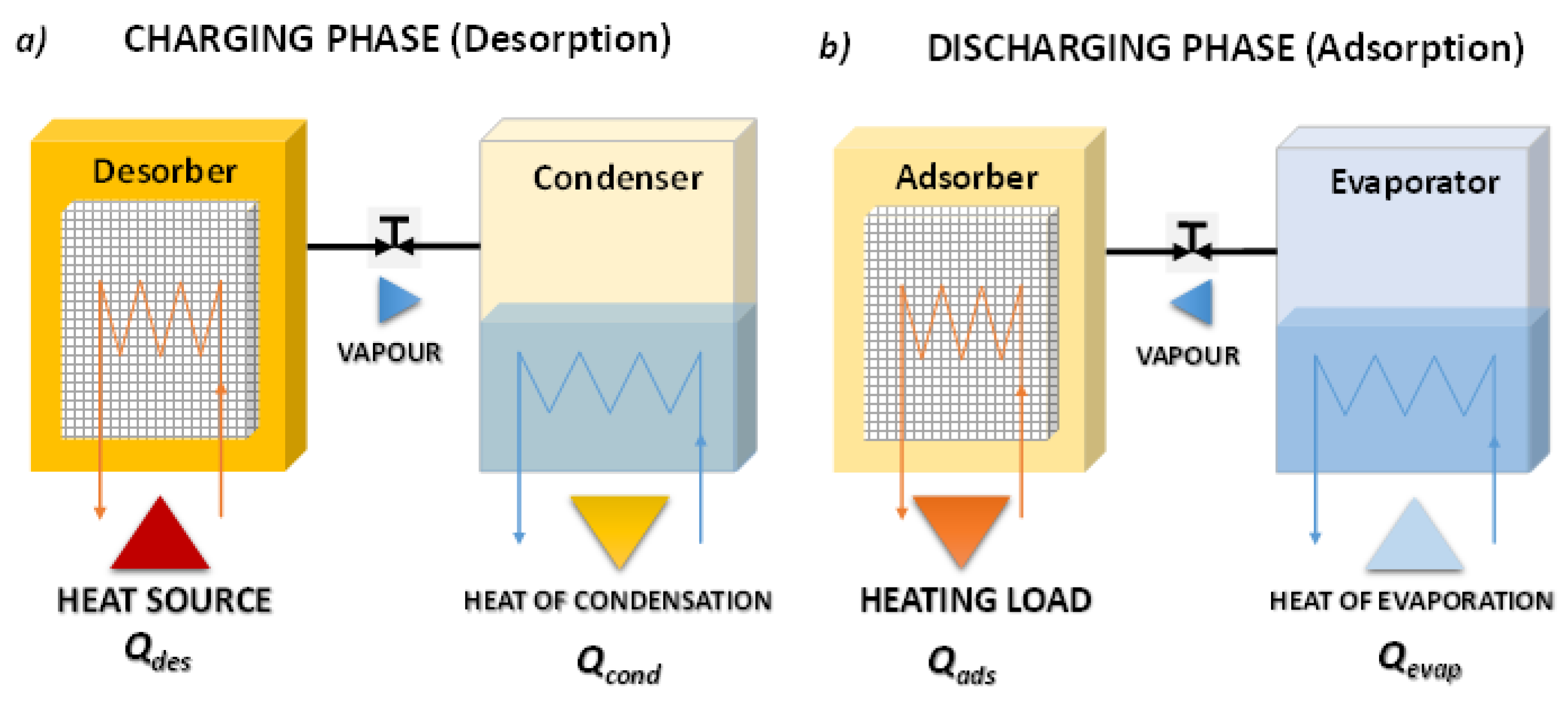
Figure 2.
The charging phase of an adsorption TES system combined with a concentrated solar field.
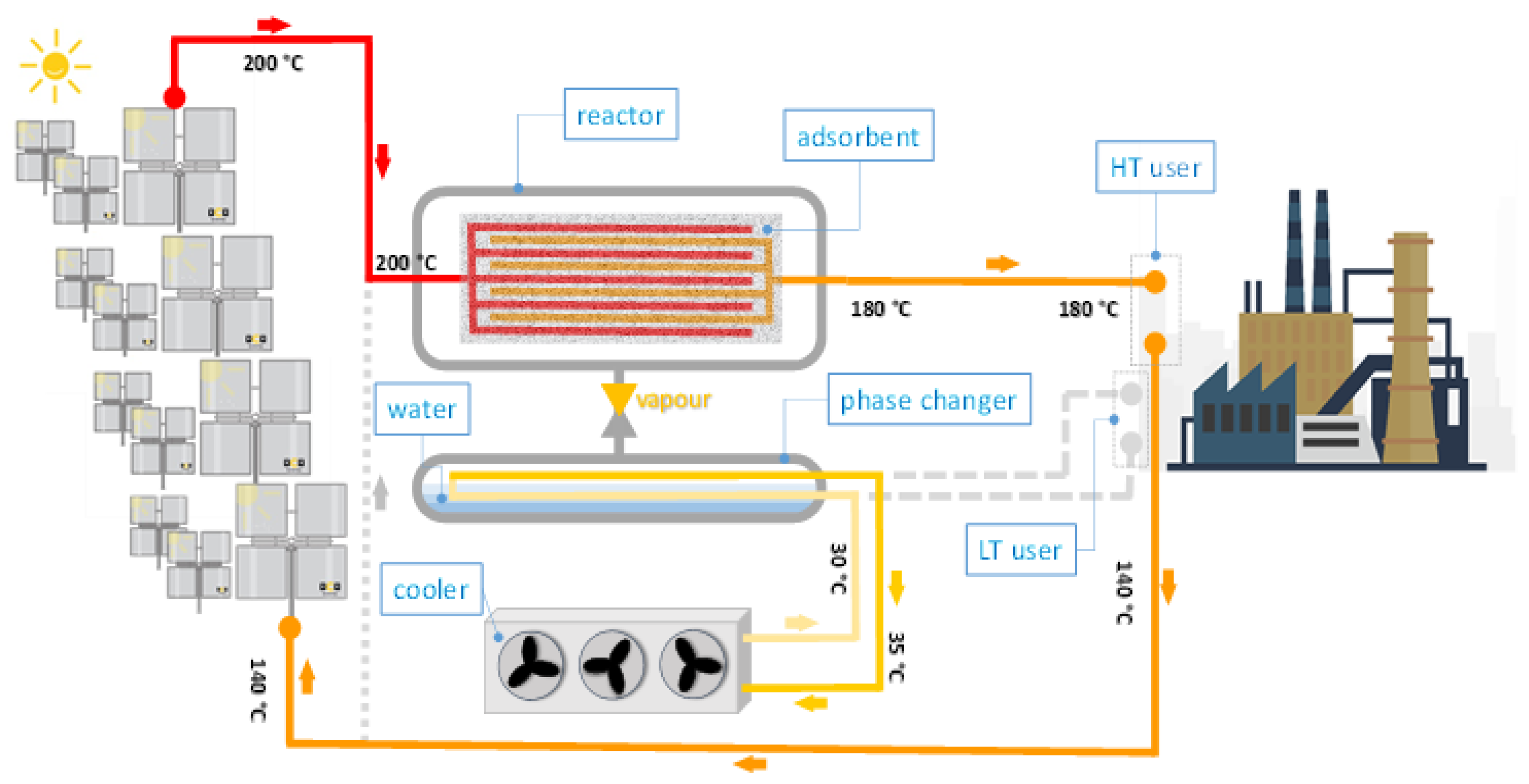
Figure 3.
The discharging phase of an adsorption TES system combined with a concentrated solar field.
Figure 3.
The discharging phase of an adsorption TES system combined with a concentrated solar field.
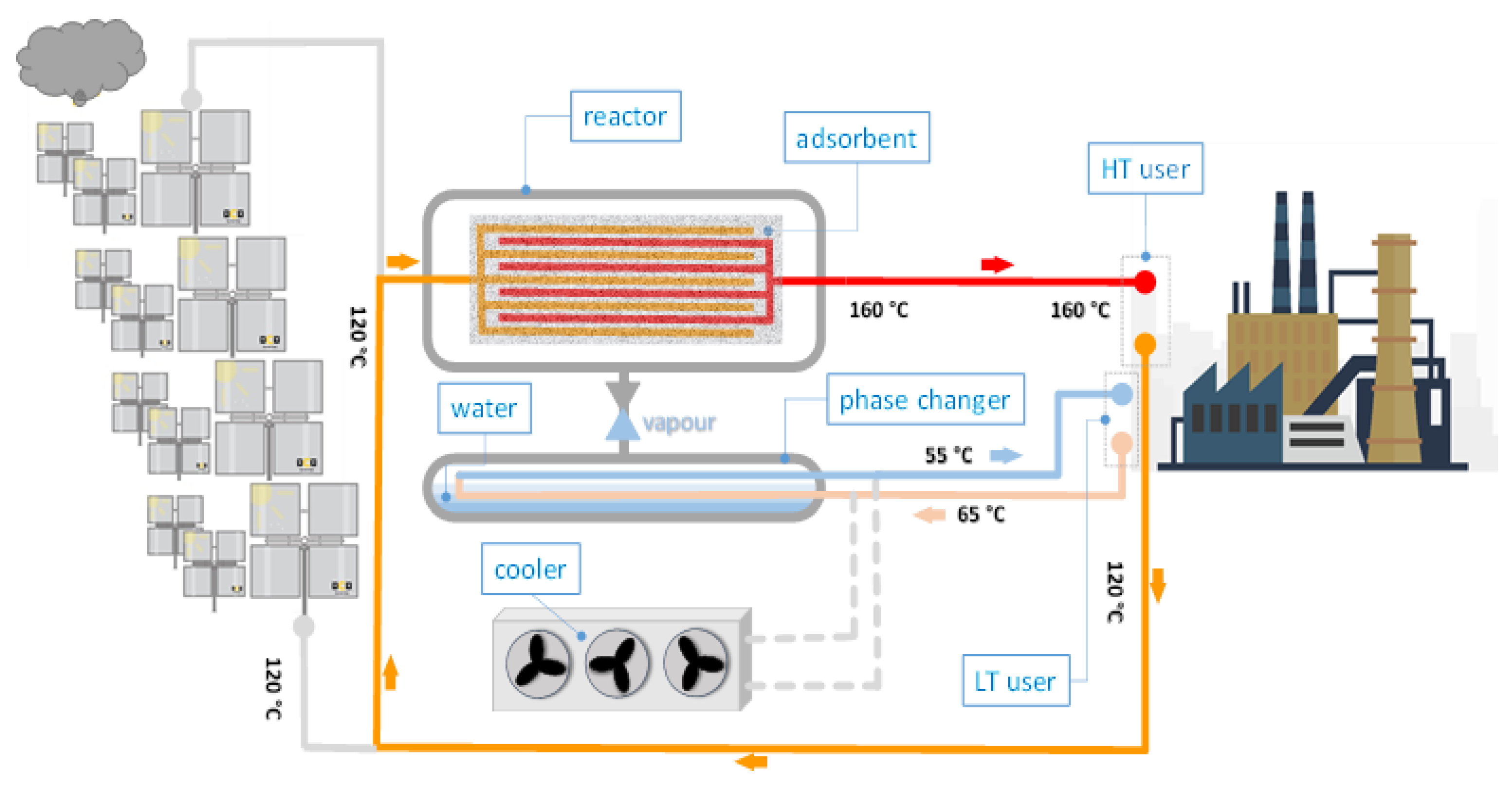
Figure 4.
Thermodynamic cycle of an adsorption storage unit.
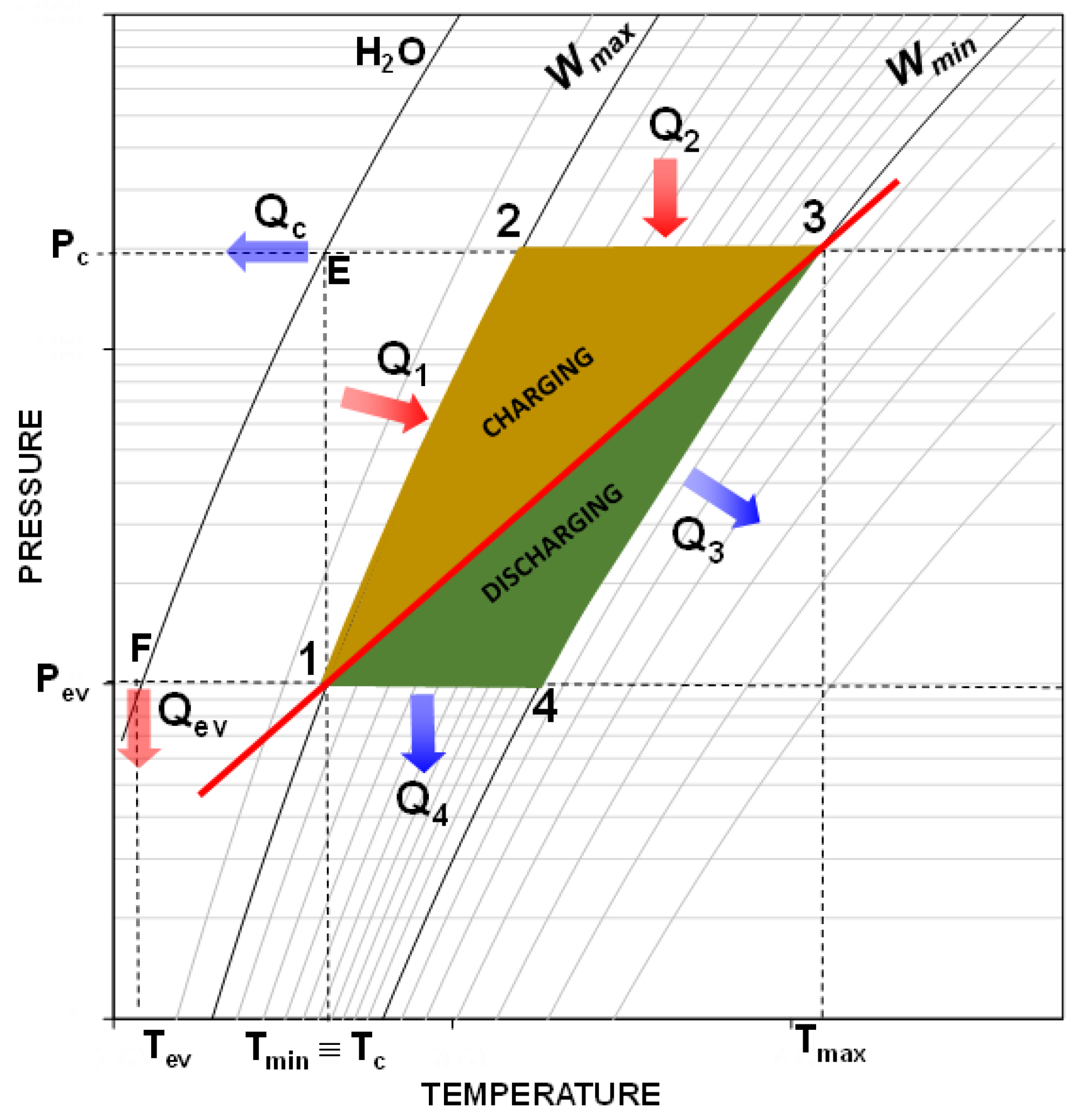
Figure 5.
Energy efficiency of short-term storage, for residential application (with ϕ = 0; 0.5; 1; 2; 3).
Figure 5.
Energy efficiency of short-term storage, for residential application (with ϕ = 0; 0.5; 1; 2; 3).
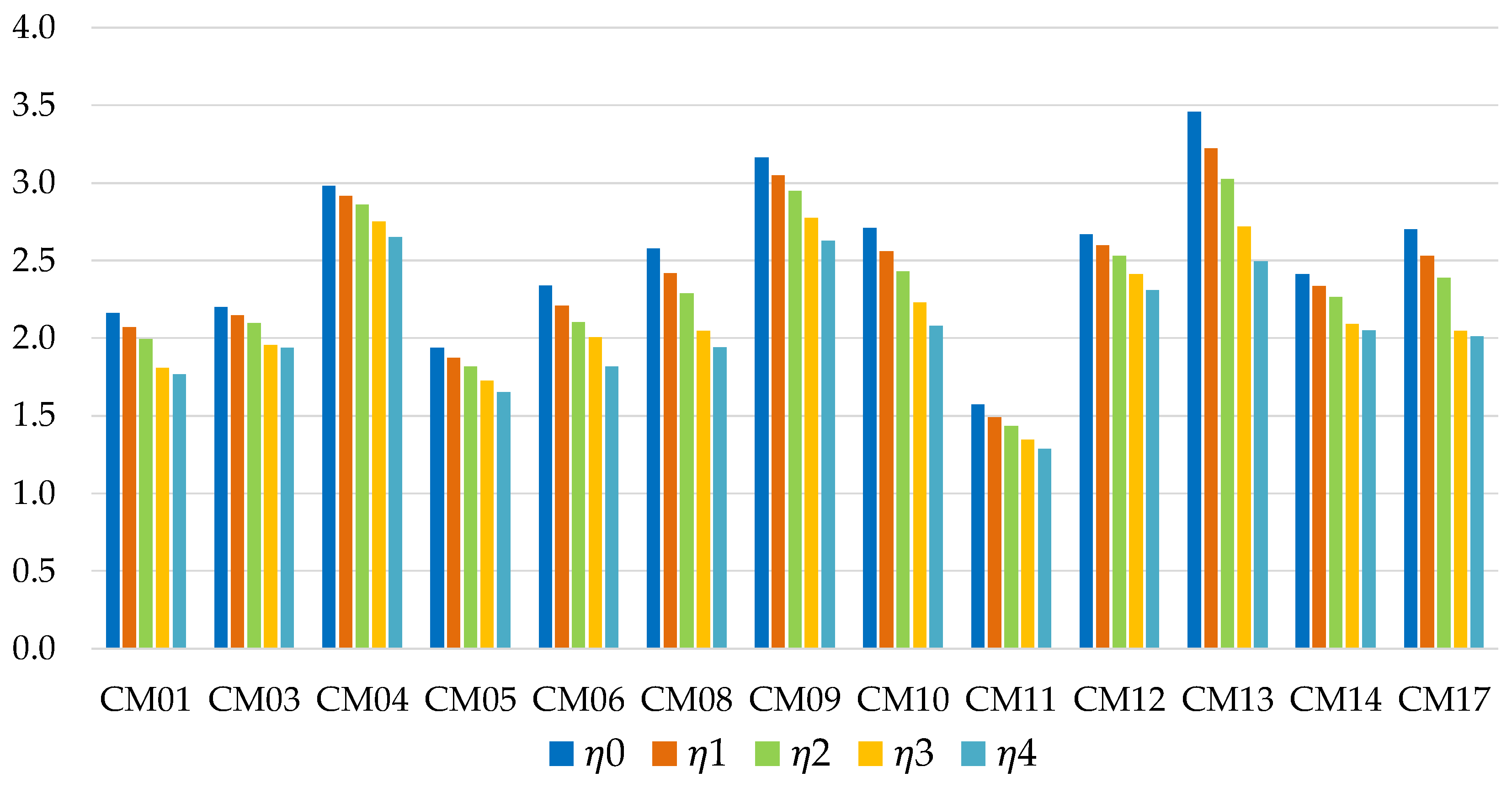
Figure 6.
Energy efficiency of long-term storage, for residential application (with ϕ = 0; 0.5; 1; 2; 3).
Figure 6.
Energy efficiency of long-term storage, for residential application (with ϕ = 0; 0.5; 1; 2; 3).
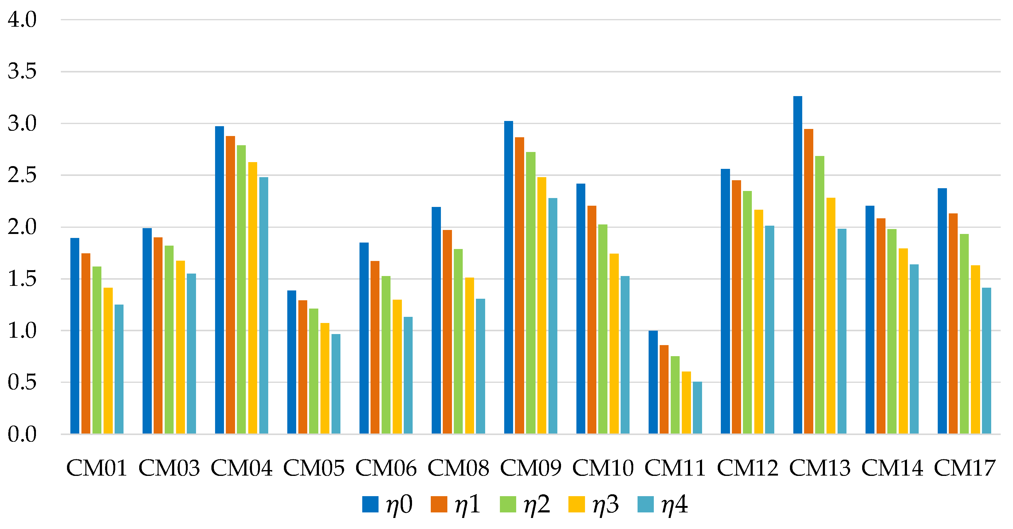
Figure 7.
Storage efficiency vs. metal/adsorbent mass ratio for residential sector: (a) short-term storage (b) long-term storage.
Figure 7.
Storage efficiency vs. metal/adsorbent mass ratio for residential sector: (a) short-term storage (b) long-term storage.
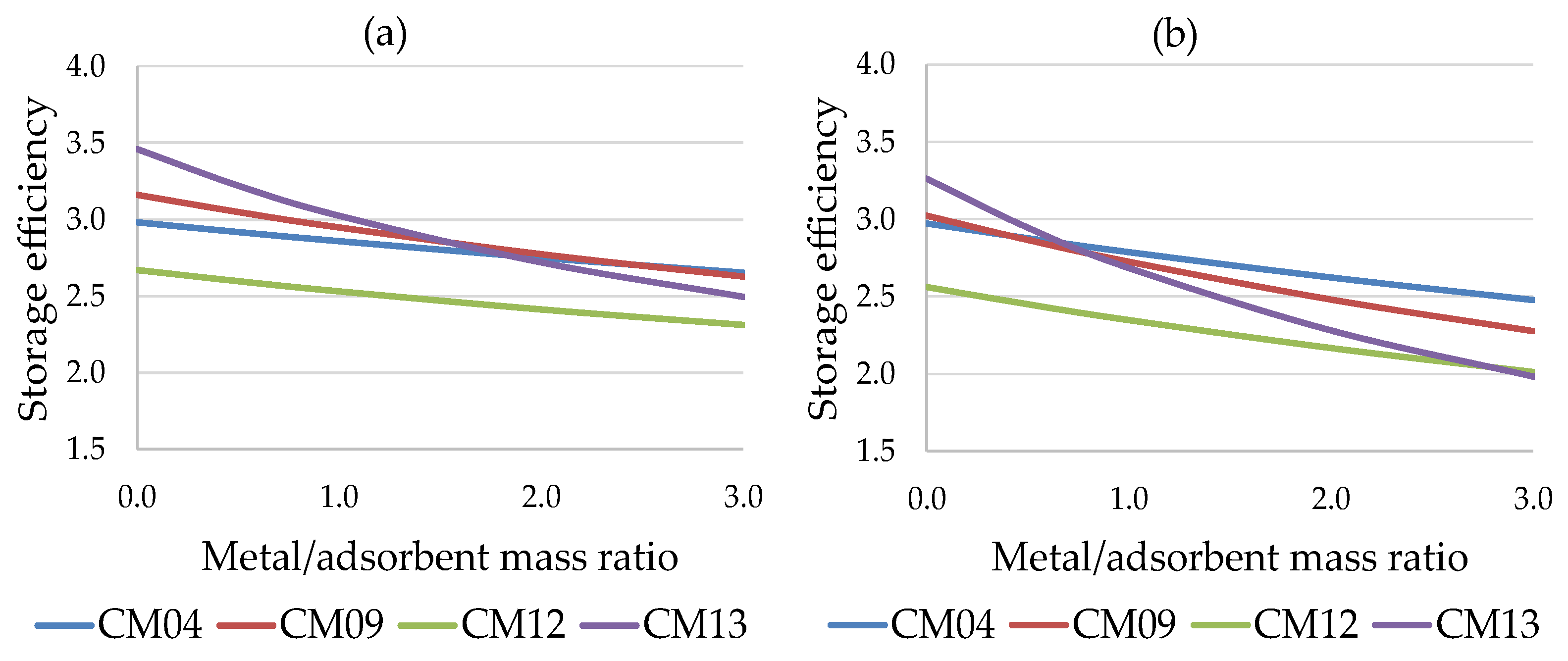
Figure 8.
Energy efficiency of short-term storage, for transport application (with ϕ = 0; 0.5; 1; 2; 3).
Figure 8.
Energy efficiency of short-term storage, for transport application (with ϕ = 0; 0.5; 1; 2; 3).
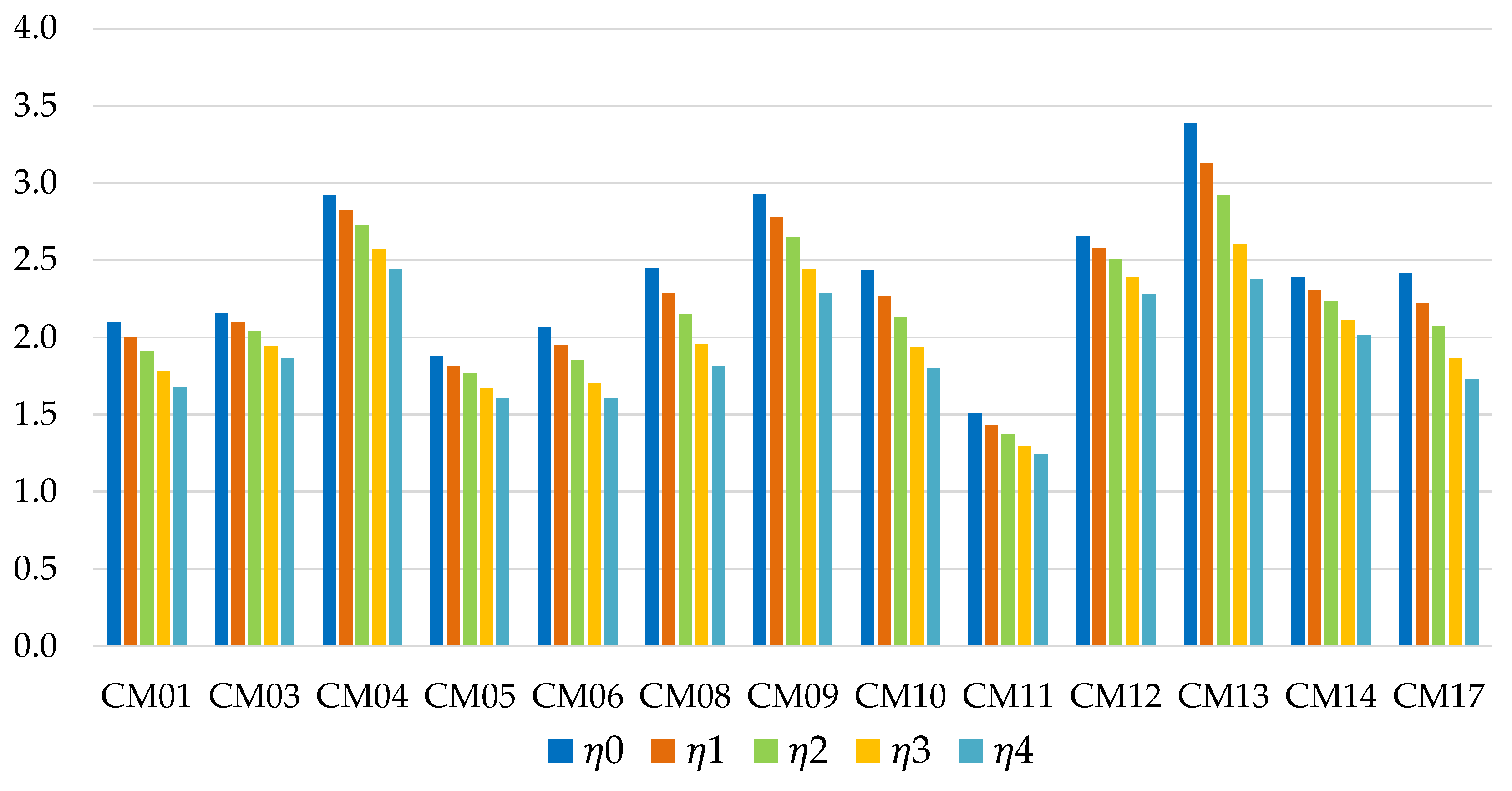
Figure 9.
Energy efficiency of long-term storage, for transport application (with ϕ = 0; 0.5; 1; 2; 3).
Figure 9.
Energy efficiency of long-term storage, for transport application (with ϕ = 0; 0.5; 1; 2; 3).
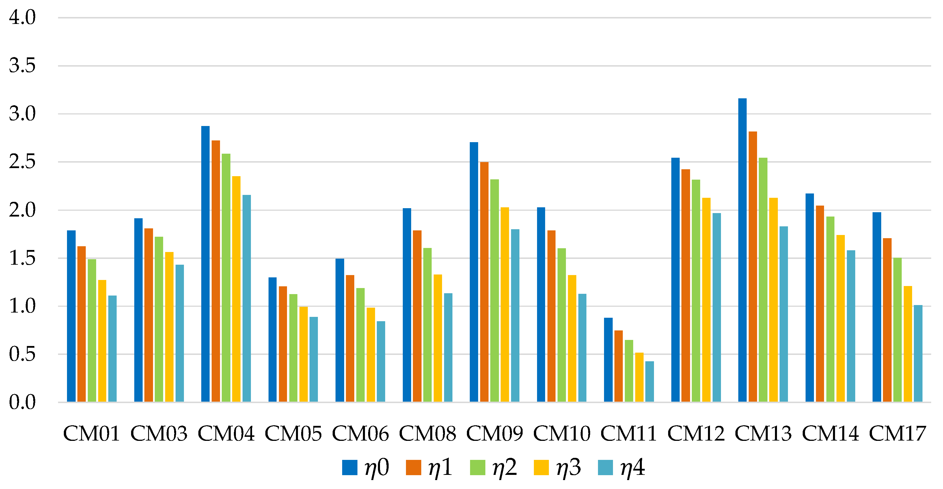
Figure 10.
Storage efficiency vs. metal/adsorbent mass ratio for transport sector: (a) short-term storage (b) long-term storage.
Figure 10.
Storage efficiency vs. metal/adsorbent mass ratio for transport sector: (a) short-term storage (b) long-term storage.
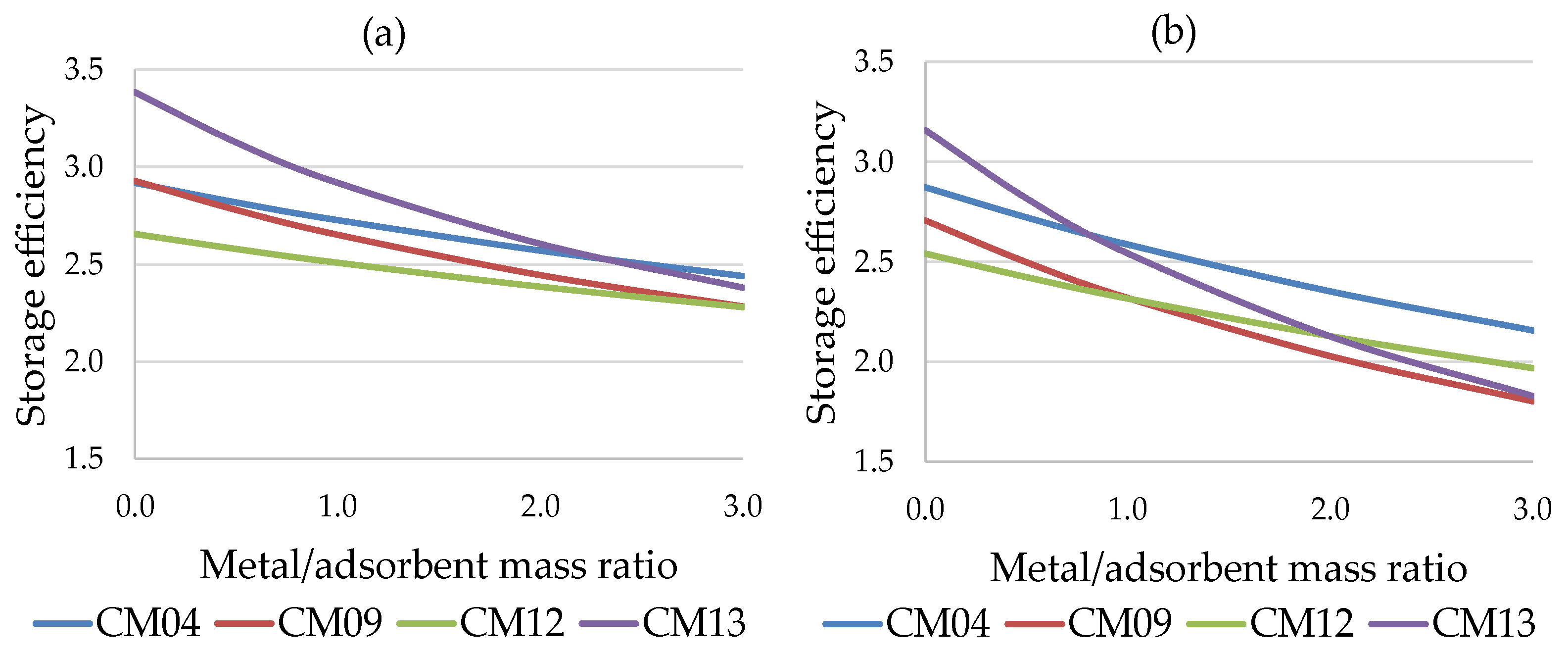
Figure 11.
Energy efficiency of short-term storage, for industrial application (with ϕ = 0; 0.5; 1; 2; 3).
Figure 11.
Energy efficiency of short-term storage, for industrial application (with ϕ = 0; 0.5; 1; 2; 3).
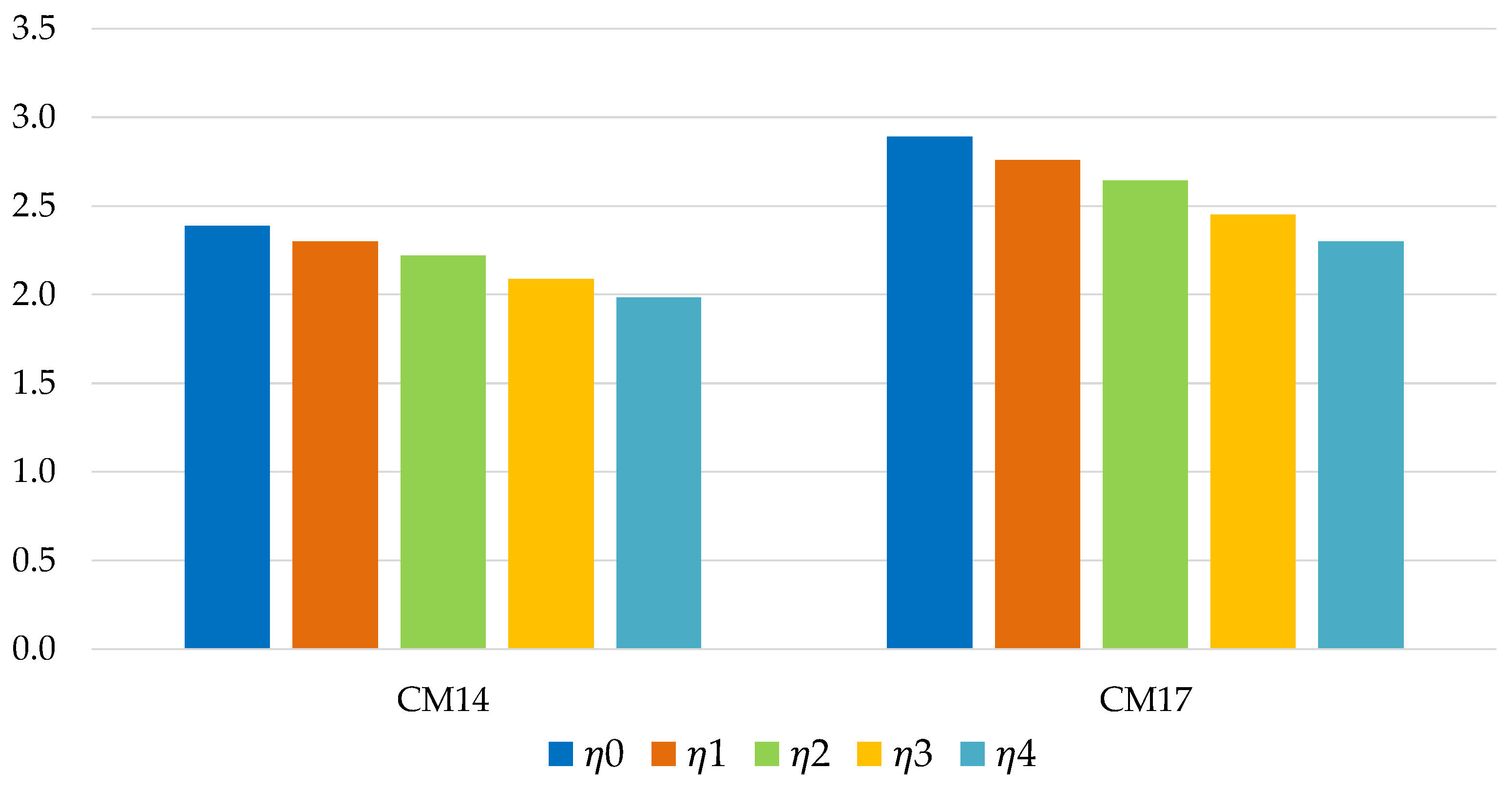
Figure 12.
Energy efficiency of long-term storage, for industrial application (with ϕ = 0; 0.5; 1; 2; 3).
Figure 12.
Energy efficiency of long-term storage, for industrial application (with ϕ = 0; 0.5; 1; 2; 3).
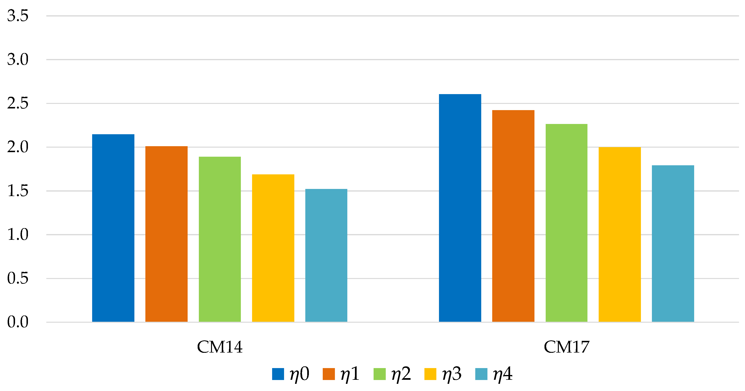
Figure 13.
Storage efficiency vs. metal/adsorbent mass ratio for industrial sector: (a) short-term storage (b) long-term storage.
Figure 13.
Storage efficiency vs. metal/adsorbent mass ratio for industrial sector: (a) short-term storage (b) long-term storage.
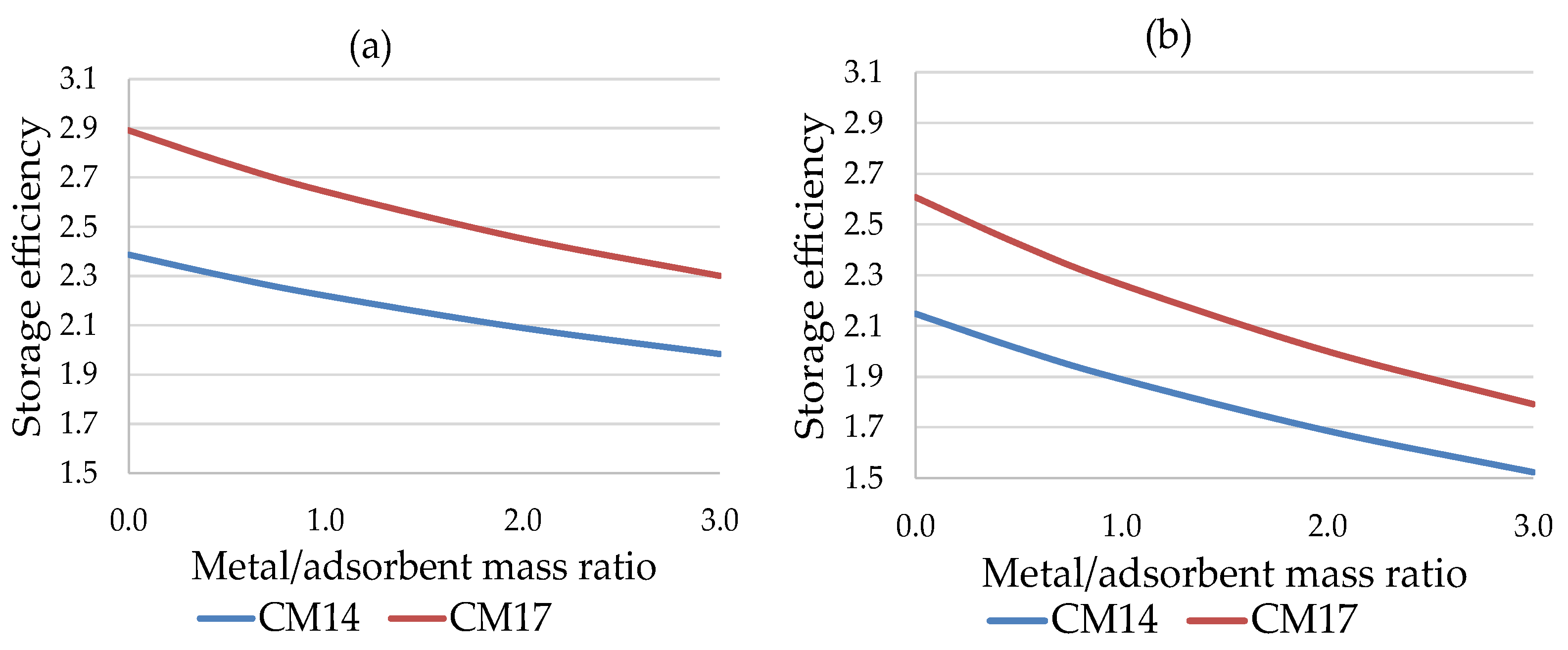

Table 1.
Boundary conditions of each application.
| Buildings | Transport | Industry | |
| Tev (°C) | 15 | 10 | 50 |
| Tcond (°C) | 40 | 40 | 60 |
| TA (°C) | 40 | 40 | 60 |
| TC (°C) | 90 | 90 | 190 |
Table 2.
Acceptable and unacceptable working pairs for the applications considered.
| Buildings | Transport | Industry | |||
| CM01 | Methanol | Activated Carbon AC35 CECA | ✓ | ✓ | × |
| CM02 | Composite CaCl2-silica | × | × | × | |
| CM03 | Composite LiBr-silica | ✓ | ✓ | × | |
| CM04 | Composite LiCl-silica | ✓ | ✓ | × | |
| CM05 | Zeolite CBV 901 | ✓ | ✓ | × | |
| CM06 | Ethanol | Activated Carbon SRD 1352/3 | ✓ | ✓ | × |
| CM07 | Carbon Fibers FR20 | × | × | × | |
| CM08 | Composite LiBr-silica | ✓ | ✓ | × | |
| CM09 | Water | Composite CaCl2-silica | ✓ | ✓ | × |
| CM10 | Composite LiBr-silica | ✓ | ✓ | × | |
| CM11 | Zeolite 4A | ✓ | ✓ | × | |
| CM12 | Zeolite AQSOA FAM Z02 | ✓ | ✓ | × | |
| CM13 | Zeolite DDZ70 UOP | ✓ | ✓ | × | |
| CM14 | Zeolite SAPO 34 Tianjin | ✓ | ✓ | ✓ | |
| CM15 | Composite Ca(NO3)2-silica | × | × | × | |
| CM16 | Zeolite AQSOA FAM Z01 | × | × | × | |
| CM17 | Silica gel Sorbsil | ✓ | ✓ | ✓ | |
Table 3.
Experimental coefficients (ai and bi) for adsorbent-adsorbate pairs.
| a0 | a1 | a2 | a3 | b0 | b1 | b2 | b3 | |
| CM01 | 20.33 | 0.0653 | -1.67E-03 | 5.24E-05 | -6003.6 | 63.15 | -2.606 | 0.0405 |
| CM02 | 15.95 | 0.2604 | -6.26E-03 | 4.83E-05 | -3616 | -72.54 | 1.831 | -0.01427 |
| CM03 | 20.19 | 0.1146 | -3.70E-05 | -2.80E-05 | -6237.4 | -9.61 | -0.106 | 9.42E-03 |
| CM04 | 17.68 | 0.2519 | -6.84E-03 | 5.26E-05 | -4358.6 | -71.03 | 2.006 | -0.0152 |
| CM05 | 16.31 | 1.366 | -1.51E-01 | 6.12E-03 | -4136.7 | -333.75 | 35.917 | -1.4372 |
| CM06 | 13.5 | 0.9116 | -3.79E-02 | 4.71E-04 | -4412.1 | -240.21 | 11.153 | -0.1412 |
| CM07 | 18.53 | -0.1591 | 9.37E-03 | -1.85E-04 | -6520.5 | 122.48 | -4.648 | 0.0786 |
| CM08 | 15.53 | 0.8438 | -3.15E-02 | 3.58E-04 | -4549.6 | -243.59 | 9.827 | -0.1075 |
| CM09 | 13.87 | 0.4646 | -1.06E-02 | 8.30E-05 | -3975.9 | -125.5 | 3.149 | -0.0248 |
| CM10 | 12.43 | 0.3657 | -5.38E-03 | 0,00 | -4101.2 | -94.02 | 1.8433 | 0.00 |
| CM11 | 14.9 | 0.9541 | -6.37E-02 | 1.85E-03 | -7698.8 | 214.98 | -18.46 | 0.5126 |
| CM12 | 14.78 | 1.3374 | -6.51E-02 | 1.17E-03 | -5329.1 | -199.59 | 7.202 | -0.0951 |
| CM13 | 8.9 | 2.2294 | -1.47E-01 | 3.34E-03 | -3266.9 | -523.4 | 35.326 | -0.8119 |
| CM14 | 15.89 | 0.8096 | -1.58E-02 | 1.33E-05 | -6113.8 | -26.57 | -7.58 | 0.2559 |
| CM15 | 20.74 | 0.082 | -6.75E-03 | 1.86E-04 | -5965 | -19.18 | 2.676 | -0.0612 |
| CM16 | 2.43 | 5.8543 | -4.87E-01 | 1.26E-02 | -109.15 | -1764.48 | 145.524 | -3.6885 |
| CM17 | 12.17 | 1.4945 | -0.07295 | 1.07E-03 | -4177.6 | -312.34 | 16.776 | -0.2501 |
Table 4.
Experimental coefficients (ci and di) for adsorbent-adsorbate pairs.
| c0 | c1 | c2 | d0 | d1 | d2 | |
| CM01 | ||||||
| CM02 | ||||||
| CM03 | ||||||
| CM04 | 0.4755 | 0.0125 | 0 | 0.0046 | 5E-6 | 0 |
| CM05 | 3.44547 | 0 | 0 | 0.00139 | 0 | 0 |
| CM06 | ||||||
| CM07 | ||||||
| CM08 | ||||||
| CM09 | 0.7111 | 4.325 | -6.662 | 1.288E-3 | 1.024E-3 | 1.1237E-2 |
| CM10 | 0.60 | 2.57 | -0.88 | 1.19E-3 | -0.104E-3 | 0 |
| CM11 | 0.82567 | 4.90113 | -5.29702 | 1.713E-3 | -9.895E-3 | 1.2272E-2 |
| CM12 | 0.7699 | 3.0641 | -4.3529 | 1.6E-3 | 7.2E-3 | 0.0403 |
| CM13 | 0.8489 | 0.0519 | -0.0007 | 0.0016 | -2.12E-05 | 6.74E-07 |
| CM14 | ||||||
| CM15 | 1.5 | |||||
| CM16 | 0.84 | |||||
| CM17 | 0.749000 | 4.18 |
Table 5.
Summary of the simulated cycles (residential sector).
| Working pair | TA (°C) |
TB (°C) |
TC (°C) |
TD (°C) |
Tcond (°C) |
Tev (°C) |
Pev=PA =PD (mbar) |
Pcond=PB =PC (mbar) |
|---|---|---|---|---|---|---|---|---|
| CM01 | 40 | 65.05 | 90 | 61.81 | 40 | 15 | 96.81 | 348.00 |
| CM02 | × | × | × | × | × | × | × | × |
| CM03 | 40 | 67.70 | 90 | 64.70 | 40 | 15 | 96.81 | 348.00 |
| CM04 | 40 | 69.29 | 90 | 56.52 | 40 | 15 | 96.81 | 348.00 |
| CM05 | 40 | 62.63 | 90 | 58.30 | 40 | 15 | 96.81 | 348.00 |
| CM06 | 40 | 61.36 | 90 | 57.22 | 40 | 15 | 42.82 | 178.26 |
| CM07 | × | × | × | × | × | × | × | × |
| CM08 | 40 | 66.86 | 90 | 62.60 | 40 | 15 | 42.82 | 178.26 |
| CM09 | 40 | 68.04 | 90 | 56.42 | 40 | 15 | 17.20 | 74.38 |
| CM10 | 40 | 72.53 | 90 | 56.33 | 40 | 15 | 17.20 | 74.38 |
| CM11 | 40 | 63.42 | 90 | 63.45 | 40 | 15 | 17.20 | 74.38 |
| CM12 | 40 | 60.90 | 90 | 63.18 | 40 | 15 | 17.20 | 74.38 |
| CM13 | 40 | 62.67 | 90 | 59.97 | 40 | 15 | 17.20 | 74.38 |
| CM14 | 40 | 60.69 | 90 | 65.60 | 40 | 15 | 17.20 | 74.38 |
| CM15 | × | × | × | × | × | × | × | × |
| CM16 | × | × | × | × | × | × | × | × |
| CM17 | 40 | 66.24 | 90 | 59.30 | 40 | 15 | 17.20 | 74.38 |
Table 6.
Summary of the simulated cycles (transport sector).
| Working pair | TA (°C) |
TB (°C) |
TC (°C) |
TD (°C) |
Tcond (°C) |
Tev (°C) |
Pev=PA =PD (mbar) |
Pcond=PB =PC (mbar) |
|---|---|---|---|---|---|---|---|---|
| CM01 | 40 | 71.05 | 90 | 56.11 | 40 | 10 | 72.78 | 348.00 |
| CM02 | × | × | × | × | × | × | × | × |
| CM03 | 40 | 71.86 | 90 | 59.53 | 40 | 10 | 72.78 | 348.00 |
| CM04 | 40 | 73.80 | 90 | 49.87 | 40 | 10 | 72.78 | 348.00 |
| CM05 | 40 | 69.64 | 90 | 51.97 | 40 | 10 | 72.78 | 348.00 |
| CM06 | 40 | 71.29 | 90 | 50.65 | 40 | 10 | 31.06 | 178.26 |
| CM07 | × | × | × | × | × | × | × | × |
| CM08 | 40 | 72.53 | 90 | 57.00 | 40 | 10 | 31.06 | 178.26 |
| CM09 | 40 | 75.36 | 90 | 49.72 | 40 | 10 | 12.38 | 74.38 |
| CM10 | 40 | 79.35 | 90 | 49.61 | 40 | 10 | 12.38 | 74.38 |
| CM11 | 40 | 69.00 | 90 | 58.01 | 40 | 10 | 12.38 | 74.38 |
| CM12 | 40 | 66.07 | 90 | 57.70 | 40 | 10 | 12.38 | 74.38 |
| CM13 | 40 | 69.77 | 90 | 53.89 | 40 | 10 | 12.38 | 74.38 |
| CM14 | 40 | 65.36 | 90 | 60.56 | 40 | 10 | 12.38 | 74.38 |
| CM15 | × | × | × | × | × | × | × | × |
| CM16 | × | × | × | × | × | × | × | × |
| CM17 | 40 | 72.66 | 90 | 53.10 | 40 | 10 | 12.38 | 74.38 |
Table 7.
Summary of the simulated cycles (industrial sector).
| Working pair | TA (°C) |
TB (°C) |
TC (°C) |
TD (°C) |
Tcond (°C) |
Tev (°C) |
Pev=PA =PD (mbar) |
Pcond=PB =PC (mbar) |
|---|---|---|---|---|---|---|---|---|
| CM01 | × | × | × | × | × | × | × | × |
| CM02 | × | × | × | × | × | × | × | × |
| CM03 | × | × | × | × | × | × | × | × |
| CM04 | × | × | × | × | × | × | × | × |
| CM05 | × | × | × | × | × | × | × | × |
| CM06 | × | × | × | × | × | × | × | × |
| CM07 | × | × | × | × | × | × | × | × |
| CM08 | × | × | × | × | × | × | × | × |
| CM09 | × | × | × | × | × | × | × | × |
| CM10 | × | × | × | × | × | × | × | × |
| CM11 | × | × | × | × | × | × | × | × |
| CM12 | × | × | × | × | × | × | × | × |
| CM13 | × | × | × | × | × | × | × | × |
| CM14 | 60 | 67.54 | 190 | 174.35 | 60 | 50 | 124.29 | 200.53 |
| CM15 | × | × | × | × | × | × | × | × |
| CM16 | × | × | × | × | × | × | × | × |
| CM17 | 60 | 70.55 | 190 | 170.25 | 60 | 50 | 124.29 | 200.53 |
Disclaimer/Publisher’s Note: The statements, opinions and data contained in all publications are solely those of the individual author(s) and contributor(s) and not of MDPI and/or the editor(s). MDPI and/or the editor(s) disclaim responsibility for any injury to people or property resulting from any ideas, methods, instructions or products referred to in the content. |
© 2025 by the authors. Licensee MDPI, Basel, Switzerland. This article is an open access article distributed under the terms and conditions of the Creative Commons Attribution (CC BY) license (http://creativecommons.org/licenses/by/4.0/).
Copyright: This open access article is published under a Creative Commons CC BY 4.0 license, which permit the free download, distribution, and reuse, provided that the author and preprint are cited in any reuse.


