
Submitted:
15 January 2025
Posted:
16 January 2025
You are already at the latest version
Abstract
The logarithmic derivative is shown to be a useful tool for data analysis in applied sciences because of either simplifying mathematical procedures or enabling an improved understanding and visualization of structural relationships and dynamic processes. In particular, spatial and temporal variations of signal amplitudes can be described independently on their sign by one and the same compact quantity, the inverse logarithmic derivative. In the special case of a single exponential decay function, this quantity becomes directly identical to the decay time constant. Generalized, the logarithmic derivative enables to flexibly describe local gradients of physical or non-physical system parameters by using exponential behavior as a meaningful reference. It can be applied to complex maps of data containing multiple superimposed and alternating ramping or decay functions as, e.g., in the case of time-resolved plasma spectroscopy, multiphoton excitation or spectroscopy. Examples of experimental and simulated data are analyzed in detail together with reminiscences on early activities in the field. Further emerging applications are addressed.
Keywords:
spectroscopy
; data analysis
; logarithmic derivative
; temporal decay
; nonlinear optics
; nonlinear order
; multiphoton processes
; pulsed lasers
; signal processing
; overlapping spectral lines
In memoriam Prof. Johannes Heinrich Hertz (April 3, 1924, Utrecht – August 26, 2010, Berlin)
1. Introduction
The spectroscopic analysis of materials or the study of the dynamics of excitation processes require to efficiently process large amounts of data at high speed. Therefore, a significant data reduction and high feature selectivity by appropriate mathematical procedures are of increasing importance for modern fields like materials research, analytical chemistry, pharmacy, medicine, plasma dynamics, laser physics or nonlinear spectroscopy. It is well known that characteristic properties of spectral data can be filtered out by mathematical derivatives [1,2]. Logarithmic differentiation is of particular interest in natural sciences and engineering because many processes follow exponential rules or contain exponential components. Prominent examples are the decay of radioactive isotopes, the spontaneous light emission of excited atoms, the discharge of capacitors, the growth of populations [3], or heat conduction [4], to mention but a few. Therefore, logarithmic derivatives often directly reveal the key parameters of functions of interest and deserve a closer consideration. For exponentially growing or decaying spatio-temporal gradients, the logarithmic derivative is constant and can be used as characteristic parameter. In dielectric relaxation spectroscopy, e.g., the logarithmic derivative is applied to calculate the real part of the complex permittivity function of multiphase or polymeric materials [5,6], or liquids [7]. Similar mathematical methods help to analyze the conduction properties of superconducting materials [8]. For the temporal analysis of diffusion [9], or for the analysis of cell growth in biology [10], the logarithmic derivative is a useful tool as well. In semiconductor physics, an inverse logarithmic derivative method is used to determine energy gaps and types of electronic transitions [11] or to simulate inelastic scattering [12]. Moreover, a logarithmic derivative lemma is applied to the solution of partial differential equations which are related to complex-valued functions with isolated pole points [13]. Another application in mathematics is to compute Bessel functions of arbitrary order [14]. In the field of mathematical statistics which has essential impact on genetics, psychology, finance etc., the score function which is based on logarithmic derivative plays a central role [15,16]. The score function is the slope of the logarithmic likelihood function the variance of which is well-known as the Fisher information [17]. The relevance of the Fisher information for fundamental physics is to link statistics to extremal principles, e.g., in diffraction optics [17,18] and quantum mechanics. The limit to the standard deviation is given by the Cramér–Rao lower bound which is related to the inverse of the Fisher information matrix [19]. The theoretical description of nuclear collisions and interactions between atoms and molecules was improved by introducing the logarithmic derivative of the wave function [20,21]. Plenty of examples give proof of the capabilities of the mathematical approach.
Moreover, the approach of logarithmic differentiation offers specific advantages from point of view of computation techniques. It simplifies the determination of derivatives of multifactorial products or quotients by transforming them into easier-to-handle sums or differences [22]. This also promises to open new prospects for efficient separation and filtering procedures. In deep machine learning, data mining, astronomical image processing and many other sectors, the logarithmic derivative is a frequently used method for clustering [23,24], or feature selection [25]. The price one has to pay for the simplification of the mathematical procedures, however, is that a differentiation sensitively responds on noise. To improve the analysis of noisy signals, most probable distributions can be selected by additional Bayesian analysis [26].
If the approach of logarithmic derivative is carefully applied, it proves to be an efficient and stimulating technique that extends the capabilities of data processing. Here, the application of the logarithmic derivative and related functions will be demonstrated for selected examples addressing temporal decay processes, the nonlinear order of multiphoton dissociation, and spectroscopy.
2. Logarithmic Derivative and a Generalized Decay Constant
The variation of a signal function f(t) in time domain can be described by appropriate time constants. For example, a single exponential relaxation process (e.g., by spontaneous emission) in a simplistic model is fully characterized by a decay time τ:
To also involve rising parts of the signal (e.g., by populating a radiative level via optical or electrical pumping), eq. (1) has to be generalized. This is possible by using the temporal logarithmic derivative which is defined as
with
The relationship between and f’ enables to differentiate functions by differentiating their logarithm:
The negative inverse of the logarithmic derivative represents a characteristic time τ* which is well suited for a specific description of signals in time domain except of the zeros of the f’(t) where the function is not defined and singularities appear:
In the special case of an exponential decay according to eq. (1), τ* is found to be a constant and identical to τ. In all other cases, however, the time dependent signal can also be described by τ* (t), independently on the sign of the time derivation (i.e., including increasing signal amplitudes). This essential extension makes the negative inverse logarithmic derivative a particularly valuable tool for the analysis of arbitrary temporal functions with exponential components.
The formalism is not restricted to the temporal domain and enables in the same way the determination of characteristic parameters of spatial, spectral or arbitrary other distribution functions of physical quantities where the time coordinate has to be replaced by corresponding parameters, respectively.
3. Examples
3.1. Time-Dependent Spontaneous Emission of Molecular Nitrogen
To understand the complex population dynamics of gas discharges, laser-induced plasma filaments, or gas lasers, relevant time resolved pump and relaxation processes have to be detected. In this case, the logarithmic derivative can be used to describe the temporal evolution of the population of a characteristic molecular level involving both population and depopulation paths. In the following we will demonstrate how the logarithmic derivate can be applied to analyze the temporal development of a diffuse volume plasma in a low-pressure nitrogen laser excited by a high-voltage electrical-discharge.
At the time of pioneering laser studies during the sixties of last century [27], nitrogen lasers were an attractive short-wavelength source because of enabling to easily construct home-made, cost-effective, highly compact devices [28,29]. Lasing at a UV wavelength of 337.1 nm corresponds to the (0,0) transition C3πu → B2πg of diatomic N2 molecules in the second positive system [30]. Further N2 laser vibrational bands were reported for transitions at 357.69 nm (0,1), 371.05 nm (2,4), 315.93 nm (1,0), 380.49 nm (0,2), 405.94 nm (0,3), 375.54 nm (1,3), 399.84 nm (1,4), and 353.67 nm (1,2) [31].
When high-power excimer lasers entered the market and solid state lasers were efficiently frequency converted, the application of nitrogen-lasers was mainly focused on pumping of dye lasers or to provide portable low-power sources for fluorescence spectroscopy and low-power materials processing [29] with repetition rates of up to some kHz and pulse durations in nanosecond or picosecond range. With the availability of femtosecond lasers, however, the remote optical excitation of air filaments moved into the spotlight [32,33,34,35,36,37] which are promising candidates for THz and MIR generation [38], as well as low-jitter laser-triggered switches [39]. Furthermore, nitrogen discharges in capillaries enable to generate x-ray lasing [40]. Motivated by such investigations, nitrogen plasma spectroscopy experienced a remarkable renaissance [41,42]. In diffuse gas discharges, the energy transfer of electrons to N2-molecules strongly depends on nonstationary plasma parameters which are tuned by gas pressure, gas mixture, time-dependent voltage, pre-ionization, electrode profile and distance, electrode material etc. [43,44]. The discharge follows the oscillation of the resonant electrical circuit formed by the capacity, inductivity and plasma resistance [45,46,47]. Simultaneous emission of up to seven laser bands in the second positive band was observed depending on discharge parameters [48].
A direct and highly resolved measurement of the time-dependent current density profile is challenging. Measurements with antennas or Rogowski coils [49] may cause distortions of the discharge or integrate over large volume. If the measurements are performed at sufficiently low gas pressure, the lifetime of the spontaneous emission of the upper level represents, in good approximation, the collision-free case and therefore should follow the upper level population. To properly sample the temporal behavior, the time constant of the detecting system has to be small compared to the characteristic time constants of discharge pumping and radiative transitions, and the electronic jitter has to be negligible as well.
Allow me a short excursion to the history. In the laboratory of Prof. Johannes Heinrich Hertz at the Central Institute for Optics and Spectroscopy (ZOS) of the Academy of Sciences in Berlin who would have had his 100th birthday in 2024, spectroscopic experiments with low-pressure nitrogen lasers were performed during the early 1980s [50]. To optimize the laser efficiency, the energy transfer from an oscillating discharge circuit to the population inversion of the laser plasma had to be analyzed. Lasing in nitrogen was of particular interest, not only because of the relative ease of construction of nitrogen lasers as pump sources for dye lasers but also because of being a cheap and available medium for testing the pre-ionization and switching dynamics of excimer lasers [51]. With thyratron-switched transversal discharges, UV pulses of 0.9 MW were obtained. To optimize the laser parameters, the time dependence of selected spectral bands was used to monitor plasma excitation and decay processes at gas pressures down to 0.7 kPa and peak voltages < 24 kV [52,53]. Figure 1 shows the time delay between the oscillating signals of voltage and spontaneous emission for a selected gas pressure of 4 kPa. Spontaneous emission was measured in small signal regime with a calibrated photomultiplier (time resolution 500 ps, detection wavelength 337.1 nm, amplification factor 107).
The detection wavelength corresponds to the laser transition is representative for the most relevant energy transfer channel for this type of laser. Amplified spontaneous emission (ASE) was suppressed to directly derive time-dependent small signal gain of (0,0) transition of the second positive system (C3πu → B2πg) of the N2 molecules. The corresponding parameters τ*(t) according to eq. (5) are compared in Figure 2.
One can see that, on the basis of the specific mathematical approach, the dynamics of the population inversion can directly be derived from the rising and falling parts of the curves of the plasma fluorescence. The interplay of electronic excitation (depending on electron density and temperature), optical transitions and fluorescence quenching (depending on pressure dependent collisions with molecules and atoms) is very complex. The influence of amplified spontaneous emission (ASE) was minimized by optically dividing the plasma in short sections. Because of low gas pressures, re-absorption was minimized as well. In this way, it was possible to determine the parameter τ* in the small signal regime. The generalized parameter describes the optical response resulting from the counteracting amplification and absorption processes in the non-thermal laser plasma in a compact manner.
In the example presented here, the effective time constants for upper laser level population are reduced down to about 10 ns which is significantly faster compared to the undisturbed lifetime of about 40 ns [54,55,56,57]. In general, replacing “time constants” by time-variant physical quantities enables for the improved simulation and optimization of time-dependent systems (e.g., pulsed gas lasers) on the basis of appropriate theoretical models.
It should be mentioned that the logarithmic derivative in time-domain was also applied to the analysis of time-dependent photoluminescence processes in semiconductors [58]. It was found that different contributions to the carrier relaxation can be separated by analyzing the logarithmic derivative in a confined polynomial model.
3.2. Nonlinear Order of Multiphoton Processes
To The intensity dependence of the multiphoton ionization (MPI) or multiphoton dissociation (MPD) processes in gas under simplifying assumptions (quasi-monochromatic excitation, exact resonance, square-wave pulses, intensity along the interaction zone, collision-free conditions) can be determined by solving the related population balance equations. At sufficiently low intensity far from saturation, with negligible background signal, and if the conversion rate is simply proportional to the intensity, the product concentration C can be assumed to depend exponentially on the excitation intensity Iexc:
where n is the nonlinear order (or exponential index). In general, n may also depend on the intensity and can be described by a modified form of a logarithmic derivation [59,60]
A particular example for a nonlinear photolytical process is presented in Figure 3 by the gas-phase multiphoton dissociation of Mo(CO)6 (molybdenum hexacarbonyl) at XeCl-laser wavelengths around 308 nm and a pulse duration of 7.5 ns. The gas pressure was stabilized at 20 Pa without additional buffer gas. The intensity dependent emission line of the molybdenum atom transition z5P0-a5S (J2=3 to J1=2, wavelength 550.649 nm [61]) is depicted in a double-logarithmic plot [62]. The maximum slope of the quasi-linear part corresponds to a nonlinear exponent of about nmax = 3.3 between laser intensities of 2.5 x 10⁸ W/cm2 and 3.3 x 10⁸ W/cm2 which indicates a sequential multiphoton excitation mechanism involving at least 3 photons. At intensities above 3.3 x 10⁸ W/cm2, saturation behavior is observed. The intensity dependent nonlinear exponents n(IL) along the entire curve can be determined by applying eq. (7). Assuming a dissociation energy of 9.44 eV for a complete release of all ligands [63,64,65] and a 3-step excitation with photon-energies of 4.03 eV, an excess energy of up to 2.59 eV can be expected (in contrast to the values reported in [62] which were calculated for a different photon energy). The experimentally detected nonlinear order widely confirms this model and an additional contribution of a 4-photon excitation channel seems to play a role.
A more detailed information on the excitation mechanisms is provided by determining the nonlinear order as a function of excitation energy (Figure 4).
The indicated nonlinear path to neutral Mo atoms and similar findings for the generation of neutral C2-radicals by the multiphoton dissociation of aromatic compounds [62] lead to the conclusion that atomic or diatomic neutral photolysis products can be obtained in appropriate parameter windows via sequential UV-multiphoton super-excitation of molecules. The parameter windows (intensity, photon energy) for the formation of such reactive and energetic non-ionic fragments are of particular interest for applications in laser-induced thin-film deposition [65,66] or MPD-pumped dissociation lasers [67]. Furthermore, the nonlinear intensity dependence on the basis of the logarithmic deviation can be exploited to determine laser parameters by analyzing the geometry of focal zones via spatial profiles of fragment fluorescence (photochemical power meter) [68,69]. The quantitative interpretation of MPD-induced fluorescence requires a careful spatio-temporal calibration.
3.3. Separation of Overlapping Spectral Peaks
The accurate analysis of spectra is essential because of identifying the chemical signature of substances, e.g., in chromatography, or to monitor chemical reactions. Often this requires a disentanglement of the contributions of overlapping spectral intensity peaks. For this purpose, numerous methods were developed which are based on approximating functions of the line shape (Gaussian, Lorentzian, Pseudo-Voigt, B-spline, Exponentially Modified Gaussian, Poisson, etc.). A comprehensive review of these techniques would exceed the frame of this paper. In many cases, however, only the positions of overlapping peaks have to be determined for a sufficiently meaningful analysis. To process spectra with idealized Gaussian or Lorentzian peaks, derivative functions from first to fourth order were applied [70,71,72,73,74,75,76,77]. It was found that the reliability of these methods is limited so that spectral peaks remain undetected or incorrect positions may be calculated [78,79]. An alternative approach for a more accurate determination of spectral peak coordinates was developed on the basis of the logarithmic derivative [80]. In this paper, the authors demonstrated that the used assumption of Gaussian shape functions (which is the necessary precondition for the mathematical procedure) enables to reliably identify peak positions independently on Lorentzian contributions.
Close to a single spectral peak, the detected spectral intensity S(λ) can be approximated by a Gaussian distribution function (probability density function):
(λ = wavelength, σ = standard deviation, µ = maximum position). The parameter σ is proportional to the half width at half maximum (HWHM)
The derivative of the natural logarithm of the assumed spectral profile according to eq. (8) enables to linearize the problem:
In ref. [79] it is shown how this procedure can easily be extended to the case of Lorentzian line shapes and approximating Gaussian distribution functions can be applied. In the case of multiple overlapping peaks, one can assume
where σi and µi are the HWHM and the positions of the individual peaks, respectively. The superposition of the peaks results in the spectral intensity function
The logarithmic derivative of this sum with respect to the wavelength can be written as
The approach linearizes the problem. Figure 5, Figure 6 and Figure 7 visualize the principle of linearization schematically for two adjacent Gaussian peaks of small spectral distance and equal maximum intensity. The existence of two peaks (Figure 5) is clearly indicated by the different slopes (Figure 6).
Eq. (13) provides the total spectral intensity of the two superposed Gaussian contributions as
The further mathematical procedure for a reliable determination of the peak positions, however, is more complicated and has to be adapted to the ratios of individual HWHMs and distances of the peaks to each other (for the details, see ref. [80]). The error of spectral resolution strongly depends on these parameters. For the example peaks in Figure 5, Figure 6 and Figure 7 it can be shown that the statistical error is too large for a reliable determination of the peak positions for realistic values of experimental noise.
In the following, the frequently occurring case of two overlapping peaks of significantly different HWHMs σ1 and σ2 will be discussed. For the sake of simplicity, it is assumed that S(µ2) = S(µ1). One expects a spectral shift of narrower peaks towards larger peaks because of the asymmetric background (Figure 8 and Figure 9). The trivial solution for a correction would be to subtract one peak to exactly determine the position of the other one. Unfortunately, the information is not a priori available in most cases. The solution can be found on the basis of the linearization by logarithmic derivation.
To determine the original peak positions, one has to solve the complete system of equations which describes the mutual influences by all neighboring spectral lines [80]. In the case of only two overlapping peaks, these equations are
and the related matrix can be written as
with the matrix elements for the exponential contributions
Solving matrix (17) enables for determining the factors (see eq. (11)) which contain the unknown HWHMs. By subtracting the contributions of the neighboring peaks, one can calculate the original spectral peak positions µ1 and µ2, respectively.
4. Conclusions
In summary, the logarithmic derivative was proven to be a simple and efficient tool for transforming scientific data to extract essential properties if the basic processes have a relationship to exponential structures in spatial, temporal or spectral domain. This was demonstrated by a few simple experimental examples. In the language of image processing, data processing with the logarithmic derivative can be interpreted as a specific kind of contrast amplification. In the particular case of temporal data, the negative inverse of the logarithmic derivative is a universal and compact descriptor for both decreasing as well as increasing functions. Here, the mathematical approach supports an unambiguous physical interpretation. A limitation of the inverse function, however, is the appearance of singularities at minima and maxima of signal functions.
In general, processing data with the logarithmic derivative procedure can be applied to any multi-dimensional data set. If this is meaningful, however, depends on the mathematical structure of the related dynamics or relationships and has to be evaluated from case to case. In physical or chemical context, some prior information on relaxation-, growth- or diffusion-type processes is often available and enables to decide if an application is appropriate. The approach could also be interesting for further tasks of signal processing like decoding of phase information in wave trains or super-resolution microscopy if a Gaussian decomposition is possible.
Author Contributions
The authors declare that no support by AI was used.
Funding
No funding to be mentioned.
Institutional Review Board Statement
Not applicable.
Informed Consent Statement
Not applicable.
Data Availability Statement
Data can be provided by the author.
Acknowledgments
The author likes to thank Dr. Martin van Moerstedt-Bock from Max Born Institute for Nonlinear Optics and Short-Pulse Spectroscopy for valuable discussions and Prof. Nathalie Picqué for the institutional support.
Conflicts of Interest
The author declares no conflicts of interest. Funding agencies had no role in the design of the study; in the collection, analyses, or interpretation of data; in the writing of the manuscript; or in the decision to publish the results.
References
- Collier, G.L.; Singleton, F. Infra-red analysis by the derivative method, J. Appl. Chem. 1956, 6, 495–510. [Google Scholar] [CrossRef]
- Dehghani, H.; Leblond, F.; Pogue, B.W.; Chauchard, F. Application of spectral derivative data in visible and near-infrared spectroscopy. Phys. Med. Biol. 2010, 55, 3381–3399. [Google Scholar] [CrossRef]
- Vandermeer, J. How populations grow: the exponential and logistic equations, Nature Education Knowledge 2010, 3(1):15. https://www.nature.com/scitable/knowledge/library/how-populations-grow-the-exponential-and-logistic-13240157/.
- Delfini, L.; Lepri, S.; Livi, R.; Politi, A. Self-consistent mode-coupling approach to one-dimensional heat transport, Phys. Rev. E 2006, 73, 060201. [CrossRef]
- Wübbenhorst, M.; van Turnhout, J. Analysis of complex dielectric spectra. I. One-dimensional derivative techniques and three-dimensional modelling, J. Non-Cryst. Solids 2002, 305, 40–49. https://www.sciencedirect.com/science/artcle/pii/S0022309302010864?via%3Dihub.
- Haspel, H.; Kukovecz, Á.; Kóny, Z.; Kiricsi, I. Numerical differentiation methods for the logarithmic derivative technique used in dielectric spectroscopy, Processing and Application of Ceramics 2010, 4, 87–93. https://iopscience.iop.org/article/10.1088/0957-0233/14/9/401/pdf.
- Kaatze, U. Logarithmic derivative complex permittivity spectrometry, Meas. Sci. Technol. 2003, 14, N55–N58. https://iopscience.iop.org/article/10.1088/0957-0233/14/9/401/pdf.
- Jurelo, A.R.; Menegotto, R.; Costa, de Andrade, A.V.C.; Junior, P.R.; da Cruz, G.K.; Lopes, C.S.; dos Santos, M.; de Sousa, W.T.B. Analysis of fluctuation conductivity of polycrystalline Er1-xPrxBa2Cu3O7-δ superconductors, Brazil. J. Phys. 2009, 39, 667–672. https://www.sbfisica.org.br/bjp/files/v39_667.pdf.
- Siems, U.; Kreuter, C.; Erbe, A.; Schwierz, N.; Sengupta, S.; Leiderer, P.; Nielaba, P. Non-monotonic crossover from single-file to regular diffusion in micro-channels, Sci. Rep. 2015, 1, srep01015. [CrossRef]
- Swain, P.S.; Stevenson, K.; Leary, A.; Montano-Gutierrez, L.F.; Clark, I.B.N.; Vogel, J.; Pilizota, T. Inferring time derivatives including cell growth rates using Gaussian processes, Nature Commun. 2016, 7, 13766. [CrossRef]
- Jarosiński, Ł.; Pawlak, J.; Al-Ani, S.K.J. Inverse logarithmic derivative method for determining the energy gap and the type of electron transitions as an alternative to the Tauc method, Opt. Mat. 2019, 88, 667–673. [CrossRef]
- Manolopulos, D.E. An improved log derivative method for inelastic scattering, J. Chem. Phys. 1986, 85, 6425–6429. [CrossRef]
- Li, B.Q. A logarithmic derivative lemma in several complex variables and its applications, Trans. Amer. Math. Soc. 2011, 363, 6257–6267. [CrossRef]
- Yousif, H.A.; Melka, R. Bessel function of the first kind with complex argument, Comput. Phys. Commun. 1997, 106, 199–206. [CrossRef]
- Fisher, R.A. On the mathematical foundations of theoretical statistics, Philosophical Transactions of the Royal Society A 1922, 222, 309–368. [CrossRef]
- Cox, D.R.; Hinkley, D.V. Theoretical Statistics (Chapman & Hall, 1974). [CrossRef]
- Frieden, B.R. Fisher information as the basis for diffraction optics, Opt. Lett. 1989, 14, 199–201. [CrossRef]
- Yang, F.; Nair, R.; Tsang, M.; Simon, Ch.; Lvovsky, A.I. Fisher information for far-field linear optical superresolution via homodyne or heterodyne detection in a higher-order local oscillator mode, Phys. Rev. A 2017, 96, 063829. [CrossRef]
- Chao, J.; Ward, E.S.; Ober, R.J. Fisher information theory for parameter estimation in single molecule microscopy: tutorial, J. Opt. Soc. Am A 2016, 33, B36–B57. [CrossRef]
- Kohn, W. Variational methods in nuclear collision problems, Phys. Rev. 1948, 74, 1763–1772. [CrossRef]
- Gonze, X.; Käckell, P.; Scheffler, M. Ghost states for separable, norm-conserving, ab initio pseudopotentials, Phys. Rev. B 1990, 41, 12264–12267. https://pure.mpg.de/rest/items/item_3323179/component/file_3513871/content.
- P. J. Schreier and L. L. Scharf, Statistical signal processing of complex-valued data – the theory of improper and noncircular signals, (Cambridge University Press, 2010), pp. 162–164. [CrossRef]
- Tsuda, K.; Kawanabe, M.; Müller, K.-R. Clustering with the Fisher Score, 16th Ann. Conf. on Neural Information Processing Systems (NIPS), Oct. 2003, paper 2292; in: Becker, S.; Thrun, S.; Obermayer, K. (Eds.), Advances in Neural Information Processing Systems 15, 729-736 (MIT Press, Cambridge, USA). https://papers.nips.cc/paper/2292-clustering-with-the-fisher-score.pdf.
- DeNoyer, L. K.; Dodd, J.G. (Eds.) Smoothing and derivatives in Spectroscopy. Handbook of Vibrational Spectroscopy (John Wiley & Sons, 2006).
- Chechile, R.A. Bayesian statistics for experimental scientists – a general introduction using distribution-free methods (MIT Press, Cambridge, 2020). https://mitpress.mit.edu/9780262044585/bayesian-statistics-for-experimental-scientists/.
- Heard, H.G. Ultra-violet gas laser at room temperature, Nature 1963, No. 4907, 667. https://www.nature.com/articles/200667a0.
- Stong, C.L. An unusual kind of gas laser that puts out pulses in the ultraviolet, Sci. Am. 1974, 230, 122–127. https://www.jstor.org/stable/24950104.
- Bergmann, A.; Jansen, S.; Christoffel, S.; Zimmermann, A.; Busch, K.; Hofmann, R. A low-cost setup for microstructuring experiments using a homemade UV laser, Am. J. Phys. 2012, 80, 260–265. [CrossRef]
- G. Herzberg, Molecular Spectra and Molecular Structure. I. Spectra of Diatomic Molecules (Van Nostrand, Princeton, 1950). https://www.scirp.org/reference/referencespapers?referenceid=2333128.
- Subhash, N.; Kartha, S.C.; Sathianandan, K. New vibrational bands in nitrogen laser emission spectra, Appl. Opt. 1983, 22, 3612–3617. [CrossRef]
- Luo, Q.; Liu, W.; Chin, S.L. Lasing action in air induced by ultra-fast laser filamentation, Appl. Phys. B 2003, 76, 337–340. [CrossRef]
- Bergé, L.; Skupin, S.; Nuter, R.; Kasparian; Wolf, J.-P. Ultrashort filaments of light in weakly Ionized, optically transparent media, Rep. Prog. Phys. 2007, 70, 1633–1713. https://iopscience.iop.org/article/10.1088/0034-4885/70/10/R03.
- Dogariu, A.; Michael, J.B.; Scully, M.O.; Miles, R.B. High-gain backward lasing in air, Science 2022, 331, 442–445. https://www.science.org/doi/10.1126/science.1199492. [CrossRef]
- Kartashov, D.; Ališauskas, S.; Andriukaitis, G.; Pugžlys, A.; Schneider, M.; Zheltikov, A.; Chin, S.L.; Baltuška, A. Free-space nitrogen gas laser driven by a femtosecond filament, Phys. Rev. A 2012, 86, 033831. [CrossRef]
- Steinmeyer, G. A breakthrough for remote lasing in air, Physics 2014, 7, 129 (Viewpoint). [CrossRef]
- López, S.; Garcia, A.; Rueda, D.; Oliva, E. 3D modeling of cavity-free lasing in nitrogen plasma filaments, Opt. Express 2023, 31, 8479–8493. [CrossRef]
- Kosareva, O.G.; Andreeva, V.A.; Shipilo, D.E.; Savel’ev, A.B.; Shkurinov, A.P.; Kandidov, V.P.; Makarov, V.A. Terahertz and mid-infrared radiation from femtosecond filaments in gases, in: K. Yamanouchi (Ed.), Progress in photon science - basics and applications, Springer Series in Chemical Physics Vol. 115 (Springer, 2017), pp. 35–43. [CrossRef]
- Rodriguez, M.; Sauerbrey, R.; Wille, H.; Wöste, L.; Fujii, T.; André, Y.-B.; Mysyrowicz, A.; Klingbeil, L.; Rethmeier, K.; Kalkner, W.; Kasparian, J.; Salmon, E.; Yu, J.; Wolf, J.-P. Triggering and guiding megavolt discharges by use of laser-induced ionized filaments, Opt. Lett. 2002, 27, 772–774. [CrossRef]
- Vrba, P.; Vrbová, M.; Bobrova, N.A.; Sasorov, P.V. Modelling of a nitrogen x-ray laser pumped by capillary discharge, Centr. Europ. J. Physics (CEJP) 2005, 3, 564–580. [CrossRef]
- Xu, H.L.; Azarm, A.; Bernhardt, J.; Kamali, Y., Chin, S.L. The mechanism of nitrogen fluorescence inside a femtosecond laser filament in air, Chemical Physics 2009, 360, 171–175. [CrossRef]
- Yao, J.; Xie, H.; Zeng, B.; Chu, W.; Li, G.; Ni, J.; Zhang, H.; Jing, C.; Zhang, C.; Xu, H.; Cheng, Y.; Xu, Z. Gain dynamics of a free-space nitrogen laser pumped by circularly polarized femtosecond laser pulses, Opt. Express 2014, 22, 19005–19013. [CrossRef]
- Kossyi, I.A.; Kostinsky, A. Yu.; Matveyev, A.A.; Silakov, V.P. Kinetic scheme of the non-equilibrium discharge in nitrogen-oxygen mixtures, Plasma Sources Sci. Technol. 1992, 1, 207–220. [CrossRef]
- Fons, J.T.; Schappe, R.S.; Lin, C.C. Electron-impact excitation of the second positive band system (C3Πu-->B3Πg) and the C3Πu electronic state of the nitrogen molecule, Phys. Rev. A 1996, 53, 2239–2247. [CrossRef]
- Persephonis, P.; V. Giannetas, A. Ioannou, J. Parthenios, and C. Georgiades, The time dependent resistance and inductance of the electric discharges in pulsed gas lasers, IEEE J. Quant. Electron. 1995, 31, 1779–1784. [CrossRef]
- Silva, A.V.; Tsui, K.H.; Pimentel, N.P.; Massone, C.A. Plasma electronics in pulsed nitrogen lasers, IEEE J. Quant. Electron. 1992, 28, 1937–1940. https://ieeexplore.ieee.org/document/144487.
- Panchenko, A.N.; Tarasenko, V.F.; Lomaev, M.I.; Panchenko, N.A.; Suslov, A.I. Efficient N2 laser pumped by nanosecond diffuse discharge, Opt. Commun. 2019, 430, 210–218. [CrossRef]
- Castro, M.P.P.; Fellows, C.E.; Massone, C.A. Simultaneous emission of seven bands in the N2 2+ system by current confinement and discharge channel plasma inductance reduction, Opt. Commun. 1993, 102, 53–58. [CrossRef]
- Rogowski, W.; Steinhaus, W. Die Messung der magnetischen Spannung. (Messung des Linienintegrals der magnetischen Feldstärke.), Archiv für Elektrotechnik 1912, 1, 141–150. [CrossRef]
- Grunwald, R.; Hertz, J.H. Über die Kleinsignalgewinnmessung nach Ladenburg-Levy (About the small signal gain measurement after Ladenburg and Levy), Ann. Phys. 1986, 498, 201–212. [CrossRef]
- Lademann, J.; König, R.; Kudryavtsev, Yu.; Albrecht, H.; Fritsch, G.; Grunwald, R.; Winkelmann, G. Ein einfacher Excimerlaser mit automatischer Vorionisation (A simple excimer laser with automatic pre-ionization), Exp. Technik d. Phys. 1984, 32, 235–246.
- Grunwald, R. Untersuchungen der spontanen Emission eines diffusen N2-laser-Plasmas (Investigations of the spontaneous emission of a diffuse N2-laser plasma), (Diploma Thesis, Humboldt University Berlin, 1982, in German).
- Grunwald, R.; Hertz, J.H. Messungen der spontanen Emission an einem diffusen N2-Laserplasma (Measurements of the spontaneous emission of a diffuse N2-laser plasma), Proceedings of 6th Conference Physik und Technik des Plasmas, Leipzig, July 5–8, 1982, 133.
- Becker, K.H.; Engels, H.; Tatarczyk, T. Lifetime measurements of the C3πu state of nitrogen by laser-induced fluorescence, Chem. Phys. Lett. 1977, 51, 111–115. [CrossRef]
- Shemansky, D.E.; Broadfoot, A.L. Excitation of N2 and N2+ systems by electrons–I Absolute transition probabilities, J. Quant. Spectrosc. Radiat. Transfer. 1971, 11, 1385–1400. [CrossRef]
- Lofthus, A.; Krupenie, P.H. The spectrum of molecular nitrogen, J. Phys. Chem. Ref. Data 1977, 6, 113–307. [CrossRef]
- Valk, F.; Aints, M.; Paris, P.; Plank, T.; Maksimov, J.; Tamm, A. Measurement of collisional quenching rate of nitrogen states N2(C3πu, v = 0) and (B2, v = 0), J. Phys. D: Appl. Phys. 2010, 43, 385202. https://hal.science/hal-00569712v1/document. [CrossRef]
- Strak, P.; Koronski, K.; Sakowski, K.; Sobczak, K.; Borysiuk, J.; Korona, K.P.; Suchocki, A.; Monroy, E.; Krukowski, S.; Kaminska, A. Exact method of determination of the recombination mode from time resolved photoluminescence data, arXiv:1709.05249v4 (2017). [CrossRef]
- Eberly, J.H. Extended two-level theory of the exponential index of multiphoton processes, Phys. Rev. Lett. 1979, 42 1049–1052. [CrossRef]
- Allen, L.; McMahon, D. The exponential index of multiphoton processes in two-photon absorption, J. Phys. B: At. Mol. Phys. 1983, 16, L721–L725. [CrossRef]
- Persistent Lines of Neutral Molybdenum ( Mo I ), Basic Atomic Spectroscopic Data, National Institute of Standards and Technology (NIST). https://physics.nist.gov/PhysRefData/Handbook/Tables/molybdenumtable3_a.htm, downloaded Oct. 23, 2024.
- Grunwald, R. Experimentelle Untersuchungen zur XeCl-Laser-induzierten stoßfreien UV-Mehrphotonendissoziation ausgewählter organischer und metallorgansicher Moleküle (Experimental investigations of the XeCl-laser induced collision-free UV multiphoton dissociation of selected organic and metal-organic molecules), PhD Thesis, Humboldt University Berlin (1986) (in German).
- Pilcher, G.; Ware, M.J.; Pittam, D.A. The thermodynamic properties of chromium, molybdenum and tungsten hexacarbonyls in the gaseous state, J. Less-Common Met. 1975, 42, 223. [CrossRef]
- Tyndall, G.W.; Jackson, R.L. Single-photon and multiphoton dissociation of molybdenum hexacarbonyl at 248 nm, J. Phys. Chem. 1991, 95, 687–693. [CrossRef]
- Radloff, W.; Hohmann, H.; Ritze, H.-H.; Paul, R. Excimer laser photolysis of molybdenum hexacarbonyl with buffer gas, Appl. Phys. B 1989, 49, 301–305. [CrossRef]
- Lenz, K.; Grunwald, R.; Weigmann, H.-J. Laser assisted deposition of carbon and polymer layers, Proceedings of the 5th International Conference on Lasers and Their Applications (ILA 5), October 28 – November 1, 1985, Dresden, Germany, 208.
- Grunwald, R.; Hertz, J.H. Nachweis eines optischen Gewinns nach UV-Mehrphotonen-Dissoziation von Molybden-Hexacarbonyl (Detection of an optical gain after UV-multiphoton dissociation of molybdenum hexacarbonyl), Ann. Phys. 1986, 7, Folge 43, No. 6-8, 499–504 (in German). https://onlinelibrary.wiley.com/doi/pdf/10.1002/andp.19864980611.
- Grunwald, R. Intensity dependent geometry of multiple photon dissociation zones, Proceedings of Lasers ’88 conference, Plovdiv, Bulgaria, Oct. 10.-14. 1988, 91–92.
- Grunwald, R. Verfahren und Anordnung zur Leistungsmessung von Laserstrahlung (Method and arrangement for measuring laser power), Patent application documents D-WP G 01 J/ 290 907 6, published Sept. 16, 1987.
- McWilliam, I.G. Derivative spectroscopy and its application to the analysis of unresolved bands, Anal. Chem. 1969, 41, 674–676. [CrossRef]
- Grushka, E.; Monacelli, G.C. Slope analysis for recognition and characterization of strongly overlapped chromatographic peaks, Anal. Chem. 1972, 44, 484–489. [CrossRef]
- Vandeginste, B.G.M.; De Galan, L. Critical evaluation of curve fitting in infrared spectrometry, Anal. Chem. 47, 2124–2134 (1975). https://opg.optica.org/as/abstract.cfm?uri=as-50-10-1235.
- Fleissner, G.; Hage, W.; Hallbrucker, A.; Mayer, E. Improved curve resolution of highly overlapping bands by comparison of fourth-derivative curves, Appl. Spectrosc. 1996, 50, 1235–1245. [CrossRef]
- J. R. Morrey, On Determining spectral peak positions from composite spectra with a digital computer, Anal. Chem. 1968, 40, 905–914. [CrossRef]
- Maddams, W.F.; Mead, W.L. The measurement of derivative i.r. spectra —I. Background studies, Spectrochim. Acta 1982, 38A, 437– 444. [CrossRef]
- Hawkes, S.; Maddams, W.F.; Mead, W.L.; Southon, M.J. The measurement of derivative i.r. spectra —II. Experimental measurements, Spectrochim. Acta 1982, 38A, 445–457. https://api.semanticscholar.org/CorpusID:95135060.
- Holler, F.; Burns, D.H.; Callis, J.B. Direct use of second derivatives in curve-fitting procedures, Appl. Spectrosc. 1989, 43, 877–882. [CrossRef]
- Griffiths, T.R.; King, K.; Hubbard, H.V.S.A.; Schwing-Weill, M.J.; Meullemeestre, J. Some aspects of the scope and limitations of derivative spectroscopy, Anal. Chim. Acta 1982, 143, 163–176. [CrossRef]
- Chen, L.; Garland, M. Computationally efficient curve-fitting procedure for large two-dimensional experimental infrared spectroscopic arrays using the Pearson VII model, Appl. Spectrosc. 2003, 57, 323–330. [CrossRef]
- A. Fernández-González, J. M. Montejo-Bernardo, Natural Logarithm Derivative Method: A novel and easy methodology for finding maximums in overlapping experimental peaks, Spectrochimica Acta Part A 2009, 74, 714–718. [CrossRef]
- Goldston, D. A.; Gonek, S. M.; Montgomery, H. L. Mean values of the logarithmic derivative of the Riemann zeta-function with applications to primes in short intervals, J. Reine Angew. Math. 2001, 537, 105–126 . [CrossRef]
- Farkas, H. M.; Godin, Y. Logarithmic derivatives of theta functions, Israel J. Math. 2005, 148, 253–265 . [CrossRef]
- Yamagata, K. Maximum logarithmic derivative bound on quantum state estimation as a dual of the Holevo bound, J. Math. Phys. 2021, 62, 062203. https://api.semanticscholar.org/CorpusID:235417320. [CrossRef]
Figure 1.
Oscillating and time delayed normalized signals of voltage (V, black squares) and spontaneous emission (SE, red circles) for a discharge pumped nitrogen gas at a pressure 4 kPa (peak voltage: 24 kV). A time delay in the range of 10 ns between excitation and emission was found.
Figure 1.
Oscillating and time delayed normalized signals of voltage (V, black squares) and spontaneous emission (SE, red circles) for a discharge pumped nitrogen gas at a pressure 4 kPa (peak voltage: 24 kV). A time delay in the range of 10 ns between excitation and emission was found.
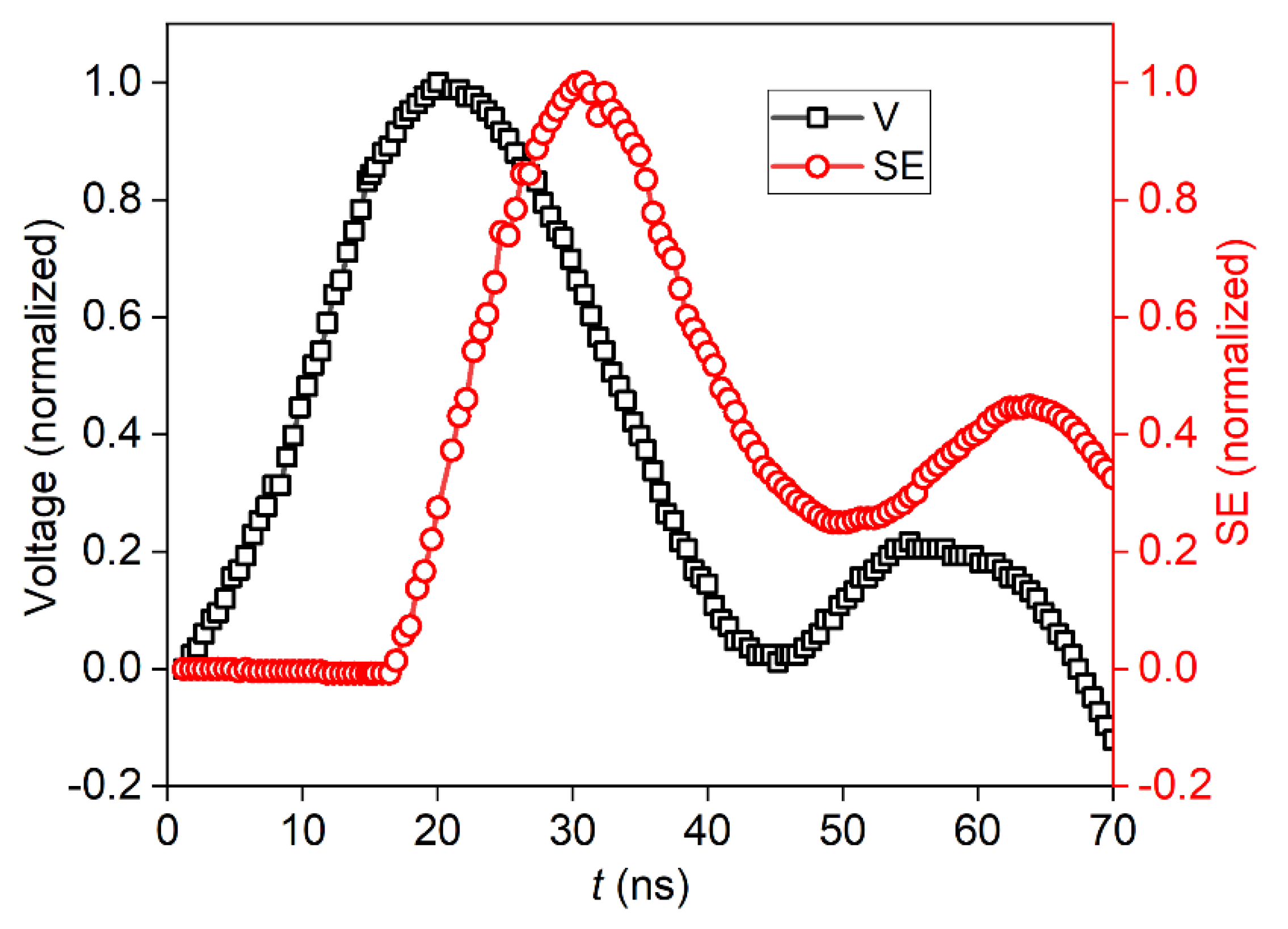
Figure 2.
Generalized time constant: The negative inverse logarithmic derivative τ*(t) of the signals in Figure 1 provides a calibrated temporal information on rising as well as decaying parts. Arrows indicate the half spaces for increasing (negative sign, at the bottom) and decreasing signals (positive sign, on top), respectively.
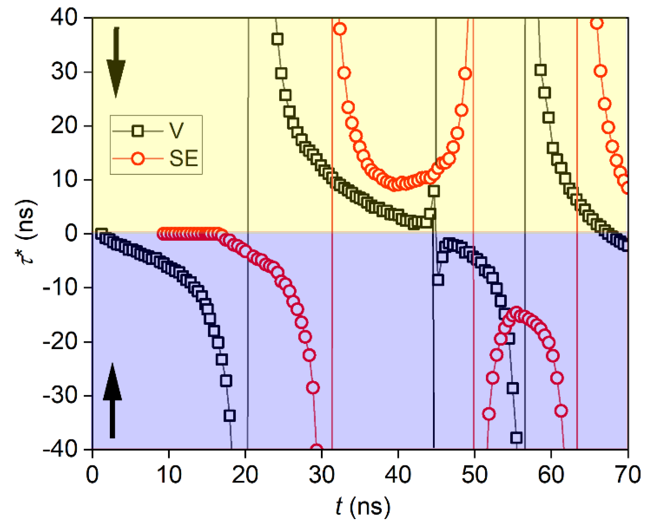
Figure 3.
Intensity dependence of the emission of neutral Mo atoms after UV-multiphoton dissociation of Mo(CO)6 in the gas phase for excitation at 308 nm and detection at 550.649 nm as a double-logarithmic plot [62]. The blue dashed line represents the slope for a maximum nonlinear order of nmax = 3.3 at excitation intensities between 2.5 x 10⁸ W/cm2 and 3.3 x 10⁸ W/cm2.
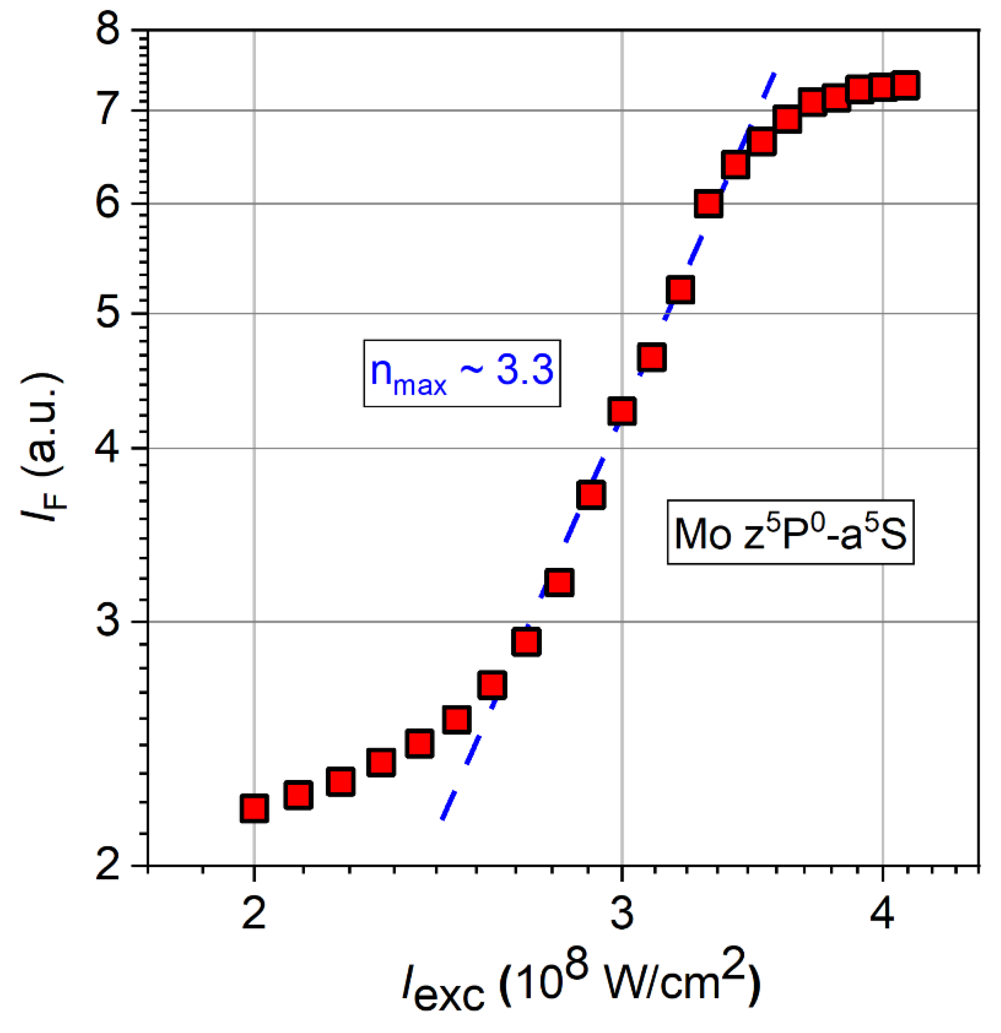
Figure 4.
Nonlinear order as a function of excitation intensity (based on experimental data used in Figure 3). The plateau corresponds to the range of most efficient generation of neutral molybdenum atoms.
Figure 4.
Nonlinear order as a function of excitation intensity (based on experimental data used in Figure 3). The plateau corresponds to the range of most efficient generation of neutral molybdenum atoms.
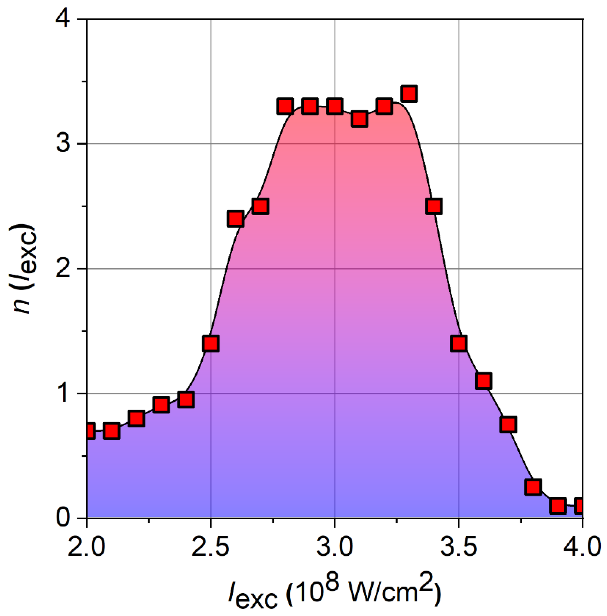
Figure 5.
Two overlapping Gaussian peaks of equal peak intensity and small spectral distance with slightly different HWHMs (σ1 = 10 nm, σ2 = 15 nm) at center wavelengths of µ1 = 500 nm and µ2 = 510 nm, respectively (numerically simulated).
Figure 5.
Two overlapping Gaussian peaks of equal peak intensity and small spectral distance with slightly different HWHMs (σ1 = 10 nm, σ2 = 15 nm) at center wavelengths of µ1 = 500 nm and µ2 = 510 nm, respectively (numerically simulated).
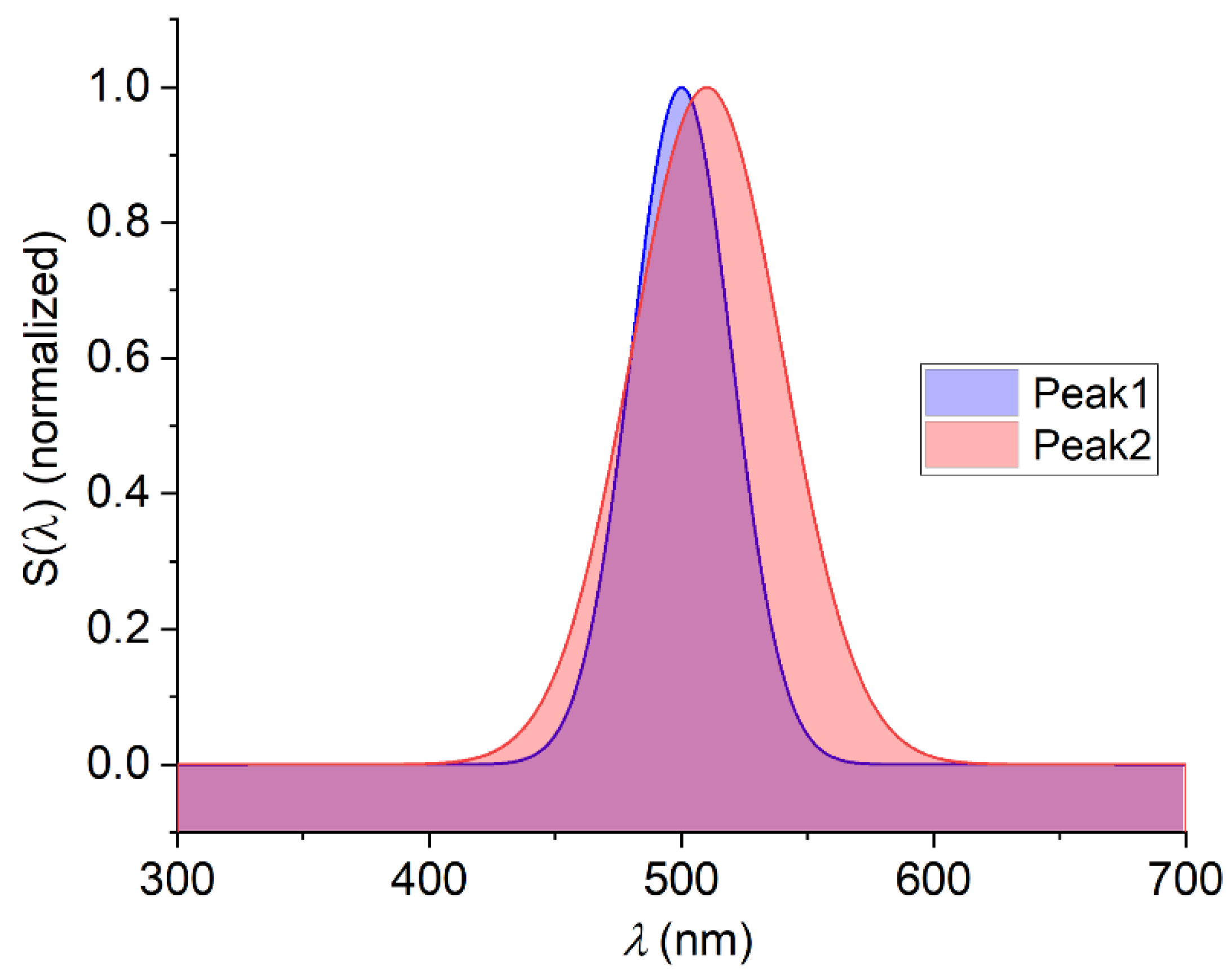
Figure 6.
Resulting total intensity according to the overlapping spectral peaks shown in Figure 5. A slight asymmetry appears. The vertical lines correspond to undistorted peak positions.
Figure 6.
Resulting total intensity according to the overlapping spectral peaks shown in Figure 5. A slight asymmetry appears. The vertical lines correspond to undistorted peak positions.
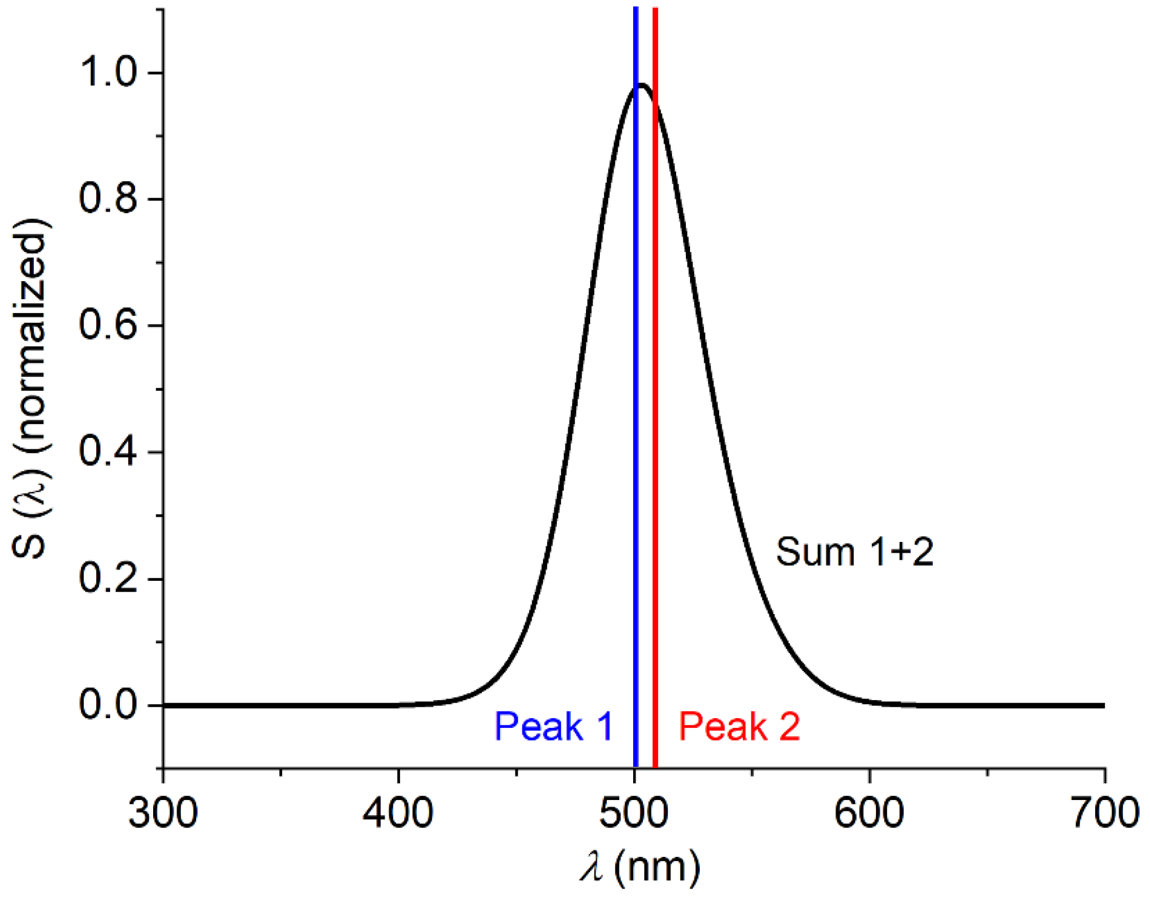
Figure 7.
Linearization of the total spectral intensity by means of the logarithmic derivative due to eq. (13). The slopes can easily be distinguished but the exact determination of peak positions requires further data processing (see ref. [80]). (For a better visualization, slope lines are shifted vertically.).
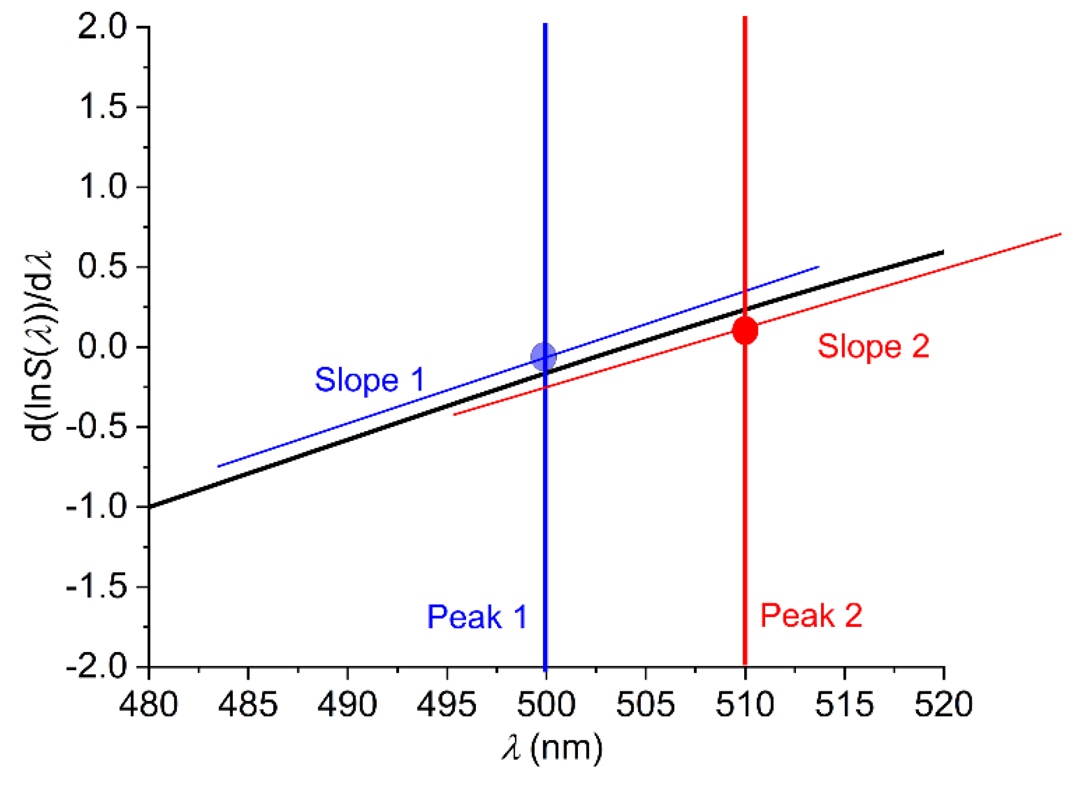
Figure 8.
Simulated superposition of two Gaussian peaks of equal intensity and significantly different HWHMs (σ1 = 200 nm, σ2 = 25 nm) located at wavelengths of µ1 = 500 nm and µ2 = 700 nm (normalized spectral intensities).
Figure 8.
Simulated superposition of two Gaussian peaks of equal intensity and significantly different HWHMs (σ1 = 200 nm, σ2 = 25 nm) located at wavelengths of µ1 = 500 nm and µ2 = 700 nm (normalized spectral intensities).
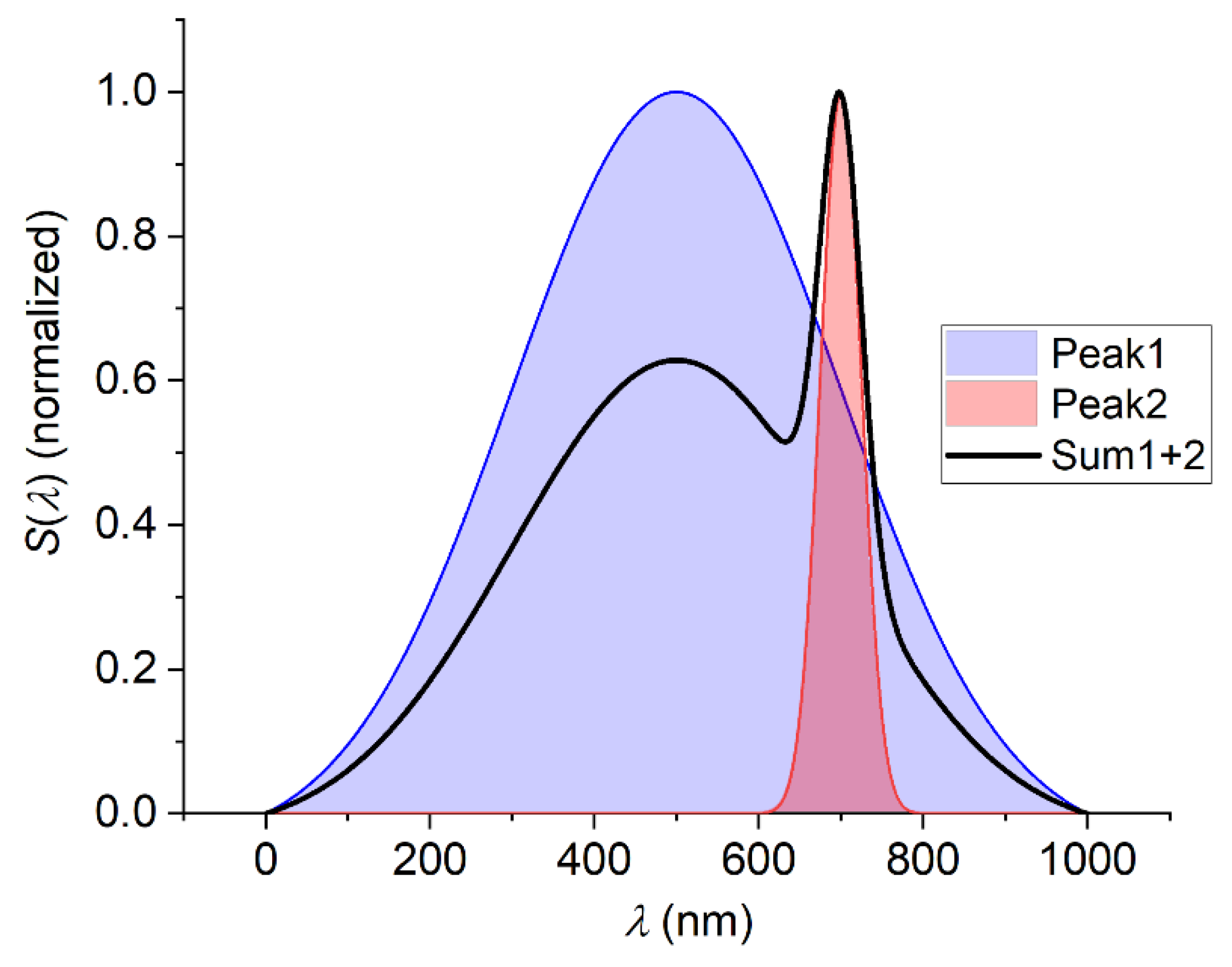
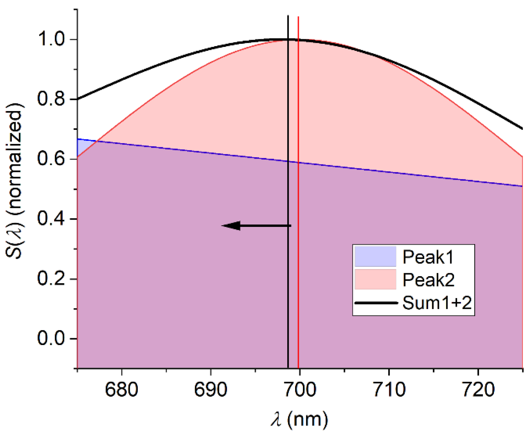
Figure 9.
Magnified region of the spectra in Figure 8 (normalized). Due to numerical simulation, the peak with smaller HWHM (peak 2) is shifted by about Δλ = 2 nm towards the peak with larger HWHM (peak 1) as a result of the asymmetric background (arrow indicates the direction of shift).
Figure 9.
Magnified region of the spectra in Figure 8 (normalized). Due to numerical simulation, the peak with smaller HWHM (peak 2) is shifted by about Δλ = 2 nm towards the peak with larger HWHM (peak 1) as a result of the asymmetric background (arrow indicates the direction of shift).
Disclaimer/Publisher’s Note: The statements, opinions and data contained in all publications are solely those of the individual author(s) and contributor(s) and not of MDPI and/or the editor(s). MDPI and/or the editor(s) disclaim responsibility for any injury to people or property resulting from any ideas, methods, instructions or products referred to in the content. |
© 2025 by the author. Licensee MDPI, Basel, Switzerland. This article is an open access article distributed under the terms and conditions of the Creative Commons Attribution (CC BY) license (http://creativecommons.org/licenses/by/4.0/).
Copyright: This open access article is published under a Creative Commons CC BY 4.0 license, which permit the free download, distribution, and reuse, provided that the author and preprint are cited in any reuse.


