
Submitted:
14 January 2025
Posted:
16 January 2025
You are already at the latest version
Abstract
Wind speed increase in pedestrian-level spaces around high-rise buildings tends to cause uncomfortable and even unsafe wind conditions for pedestrians. Especially, instantaneous strong winds can have a significant impact on the body sensation of pedestrians, and they are usually related to complex flow patterns around buildings. A detailed examination of flow patterns corresponding to instantaneous strong wind events around high-rise buildings is essential to understand the physical mechanism of this phenomenon. To quantitatively evaluate the pedestrian-level wind environment around high-rise buildings, two important indices, speed-up ratio and speed-up area, have usually been introduced. In this study, Large Eddy Simulation (LES) was conducted for square-section building models with different heights H (=100m, 200m and 400m in full-scale) or aspect ratios H/B0 (=2, 4 and 8). Two instantaneous strong wind events providing “maximum speed-up ratio” and “maximum speed-up area” of pedestrian-level wind are investigated based on a conditional-average method. Results indicate that these two instantaneous strong wind events usually do not occur simultaneously. Flow patterns around buildings for the two events are also different: the contribution of downwash tends to be larger for strong wind events providing “maximum speed-up area” showing more three-dimensional characteristics.
Keywords:
flow patterns
; pedestrian-level wind
; strong wind events
; conditional average
; high-rise buildings
1. Introduction
It is known that wind speed increase in pedestrian-level spaces around high-rise buildings tend to cause uncomfortable and even unsafe wind conditions for pedestrians [1,2]. Especially, instantaneous strong winds can have a significant impact on the body sensation of pedestrians, because they provide an indication of the maximal speed that a pedestrian might experience due to unsteady wind flow, and its unexpected nature can affect pedestrian wind comfort more and easily catch people off guard [3,4,5]. Instantaneous strong winds at pedestrian level are usually related to complex flow patterns around buildings. Therefore, a detailed examination of flow patterns corresponding to instantaneous strong wind events around high-rise buildings is essential to understand the physical mechanism of this phenomenon.
Referring to some previous studies on airflows around buildings and pedestrian wind environments, the physical mechanisms of wind speed increase at pedestrian level around buildings are considered to be Venturi effect and the downwash effect. The former originally states that a fluid’s velocity increases when the cross section of a certain mass of fluid decreases along with its passage in fluid dynamics and is usually only used for confined flow in closed channels. Currently, Venturi effect is also used in wind engineering and urban aerodynamics with the meaning of increase in wind speed due to flow constriction [6,7,8] and is typically associated with passages between buildings. In a broad sense, the term “Venturi effect” can be used even for isolated buildings, since narrower paths on two sides of an isolated building than the upstream region causes speed-up phenomenon [9,10].
The latter, downwash effect, generally happens when the approaching boundary layer flows are blocked by the windward surface of a building, causing downwash (or downward flows) on the front and two sides of the building and then accelerate the near-ground flows. Cook [11] concluded that the downward movement of the airflow is mainly due to the pressure gradient between different heights within the windward surface of the building because of wind speed difference in the approaching boundary layer flow, based on comparison of the distribution of surface wind pressure and flow field around a two-dimensional rectangular building model between a uniform turbulence flow (UTF) and a boundary layer flow (BLF). Blocken and Carmeliet [12] explained that two pressure systems determined the flow patterns around a single rectangular building based on the wind tunnel measurement results of Beranek [13]. The first one acts on the windward surface of the building with maximum pressure at the stagnation point and lower pressures on the rest of the surface due to approaching wind speed increase with height and causes a standing vortex that feeds the corner streams. The second one consists of an overpressure zone on the windward side of the building and an under-pressure zone on the leeward side, which causes reverse flow and also contributes to the corner streams [12,13]. It is obvious that the distribution characteristics of surface wind pressure are closely related to flow patterns, especially downwash effect, around buildings. Therefore, it is also necessary to examine the distribution characteristics of a building’s surface wind pressure along with flow patterns corresponding to instantaneous strong winds at pedestrian level around the building.
To quantitatively evaluate the pedestrian-level wind environment around a high-rise building, two important indices, speed-up ratio and speed-up area, have usually been introduced. The concept of speed-up ratio was introduced by Sexton [14] and defined as the ratio between the wind speed at a point around a building and the wind speed at the same point without the existence of a building. Speed-up area is the area of regions where wind speeds increase or speed-up ratio is larger than 1 and is usually near the building corners of the windward side. The magnitude of speed-up ratio reflects the influence degree of a building on the near-ground flow at a certain position. In contrast, the magnitude of speed-up area shows the actual area of high wind speed at pedestrian level around a high-rise building. Tamura et al. [9] found that downwash effect has a greater impact on the expansion of mean speed-up area around an isolated building than Venturi effect, but is comparable to Venturi effect for the maximum mean speed-up ratio, based on measured mean pedestrian-level wind speeds around square-section high-rise buildings with different dimensions (height, width, size) under BLF (Boundary layer flow) and UTF (Uniform turbulence flow) in a wind tunnel.
In this study, Large Eddy Simulation (LES) was performed for isolated high-rise buildings with different heights/aspect ratios to further examine flow patterns around buildings and distribution characteristics of building surface pressure corresponding to instantaneous strong wind events at pedestrian level providing two conditions of “maximum speed-up ratio” and “maximum speed-up area”.
2. Description of Numerical Simulation
2.1. Model Configurations
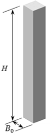
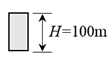
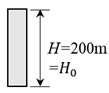
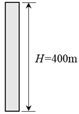
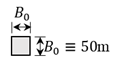
LES was conducted for three square-section buildings with the same width ( in full-scale) but different heights (, 200m and 400m in full-scale), giving aspect ratios , 4 and 8, as shown in Table 1. Here, the building model with height is defined as “reference building model (RBM)”.
2.2. Numerical Setting
The open-source Computational Fluid Dynamic (CFD) code, OpenFOAM (v8), was used. Table 2 lists the calculation conditions for LES. Referring to the commonly used CFD guidelines [15,16], the building width was uniformly discretized into 20 grids, and sufficient distances between building surfaces and boundaries of the computational domain were ensured, in which the cross-section of the computational domain corresponds to the wind tunnel section () of the PIV (Particle Image Velocimetry) test in Lin et al. [17], as shown in Figure 1(a). The mesh stretching ratio was set to 1.08 or less.
The inflow fluctuations were generated by an artificial generation method [18]. Figure 1(b) shows the approaching flow profiles obtained from LES results in an empty computational domain. It can be seen that the turbulence characteristics of the inflow boundary condition were sufficiently maintained and they show good agreement at both the inlet boundary and the origin “O”. The mean wind speed at pedestrian-level () and the top of the RBM () are equal to and , and will be used for normalization in the latter analysis. The power-law exponent of mean wind speed profile was , representing the urban terrain condition. For more information on detailed numerical settings and validation of flow fields around building models from LES based on PIV (Particle Image Velocimetry) measurements, readers can refer to Lin et al. [17].
2.3. Validation of Surface Pressure from LES
Validation of flow fields around building models from LES have been conducted based on PIV measurements in Lin et al. [17], but where building surface pressures were not measured simultaneously. Therefore, in order to validate the accuracy of surface pressures obtain from LES, the pressure coefficients are compared with the wind tunnel experimental results for a square-section building model (Full-scale height , Width ) from the TPU (Tokyo Polytechnic University) database [19]. In this Section 2.3, the subscript “” is added to the parameters to represent the LES results corresponding to the target building model in the TPU database to distinguish them from the LES results used for the latter formal analysis. The pressure coefficient is defined as
where is air density, is the reference pressure set to zero at the outlet boundary and is the mean wind speed at the top of the building model. Mean and standard deviation (std) of statistics of wind pressure coefficients is denoted as and .
The numerical simulation uses the same geometrical scale of 1/400 as the TPU wind tunnel test. It is worth mentioning that the numerical settings for LES are the same as those in Lin at al. [17] except in the computational domain that is equal to , where the cross section is equal to that of the TPU wind tunnel (). Figure 2 compares the approaching flow conditions with those in the TPU wind tunnel test. It can be seen that mean wind speed and turbulence intensity show good agreement, as shown in Figure 2(a). The power spectrum density functions of fluctuating velocities were not reported and are assumed to follow the von Karman spectrum model for the TPU database results. Therefore, the non-dimensional power spectrum density of velocity component at building height obtained from LES is compared with the Karman spectrum (Figure 2(b)), where , , and denote frequency, power spectral density, turbulence scale and standard deviation (std) of velocity component. LES results for generally show good agreement where the normalized frequency is smaller than about 1, which is determined by the computational mesh size.
Figure 3 shows variations of mean and fluctuating (std) wind pressure coefficients, and , around the perimeter of a building at obtained from LES and wind tunnel experiment (Exp.). It is observed that LES results are basically in agreement with experimental results, although LES results on the windward surface are slightly overestimated for mean pressure coefficients and slightly underestimated for fluctuating wind pressure coefficients . Figure 4 compares mean and fluctuating wind pressure coefficients for all the pressure monitoring taps on building surfaces (windward, side, and leeward surfaces) from LES and experimental results in the form of scatter plots. It can be seen that for the mean and fluctuating wind pressure coefficients, the differences between the results from LES and wind tunnel experiment are almost all in the range of . The contour plots in Figure 5 also demonstrate the good agreement and acceptable accuracy for LES results compared with experimental results.
. (a) Mean ; (b) Fluctuating ; (b) Fluctuating ; (b) Fluctuating
3. Definition of Instantaneous Strong Wind Events
In this study, we focus on two instantaneous strong wind events at pedestrian level in full-scale) around buildings providing “maximum speed-up ratio” and “maximum speed-up area”. Instantaneous speed-up ratio at time is defined as ,where , and represent instantaneous velocity components in the x, y and z directions at pedestrian level around a building.
Maximum instantaneous speed-up ratio at pedestrian level around a building occurs at a point near the building corner denoted as Point “G”, as shown in Figure 6(a). Figure 7(a) further shows the time history of instantaneous speed-up ratio at Point “G”, . Instantaneous strong wind events at pedestrian level around a building generally coincide with considerably low-occurrence frequencies. Meanwhile, wind speeds larger than 90th percentile values are generally considered to represent rare but instantaneous strong wind events in pedestrian wind environmental studies (e.g., [20,21,22]). Meanwhile, in order to reduce the risk caused by instantaneous strong wind at pedestrian-level, several wind environment criteria [3,23,24,25] have also been proposed based on a combination of threshold wind speeds and the probabilities of exceeding the corresponding thresholds. In the present study, to capture strong wind events at pedestrian level and to avoid too few data to be lack of representation, the moments when fall within the top 2% of all time-history data (red line in Figure 7(a)) are extracted. Averaged value for the top 2% approximately represent the strong wind event providing “maximum speed-up ratio” of pedestrian-level wind around a building and is denote as .
The time history of instantaneous normalized speed-up area is shown in Figure 7(b), where represents the total area surrounded by the contour line of wind speed ratio (Figure 6(b)). In the present study, a moderate value of was selected and correspondingly, the time history of instantaneous normalized speed-up area is denoted as . Similarly, the moments when falls within the top 2% of all the time-history data (red line in Figure 7(b)) are extracted. The averaged value for the top 2% approximately represents the strong wind event providing “maximum speed-up area” around a building and is denoted as . Correspondingly, three-dimensional flow fields around buildings and wind pressure coefficients on building surfaces for the two strong wind events are extracted to obtain a conditional average.
4. Simulation Results and Analysis
In this section, conditional-average results will be discussed in detail. It is worth mentioning that the definition of pressure coefficient used in the following analysis is a little different from that in Section 2.3. Here, for convenience of comparison between buildings with different height or aspect ratio , the pressure coefficient is defined as
where is the mean wind speed at the top of the “refence building model (RBM)” with aspect ratio , and .
4.1. Determination of Data Acquisition Period
In numerical simulation, the data acquisition period is usually determined based on the statistical stability of the data of interest and the computational cost of the simulation. In this paper, in order to determine the appropriate data acquisition period, the effect of data acquisition period on the probability density distributions and percentile values of and is mainly discussed and shown in Appendix A. It is shown that a data acquisition period of 20min or 1200s in full scale is sufficient to ensure acceptable uncertainty.
4.2. Conditional-Average Results
As shown in Figure 7, it can be seen that the moments corresponding to “maximum speed-up ratio” event and “maximum speed-up area” event mostly do not coincide for the building model with aspect ratio . A similar phenomenon can also be seen for other building models with different heights H or aspect ratios and 8, as shown in Figures. 8 and 9. This phenomenon indicates that the two strong wind events do not occur simultaneously.
Figure 9.
Extraction of maximum-level of speed-up ratio and normalized speed-up area at pedestrian level around the building model with aspect ratio . (a) “Maximum speed-up ratio” event, ; (b) “Maximum speed-up area” event
Figure 9.
Extraction of maximum-level of speed-up ratio and normalized speed-up area at pedestrian level around the building model with aspect ratio . (a) “Maximum speed-up ratio” event, ; (b) “Maximum speed-up area” event
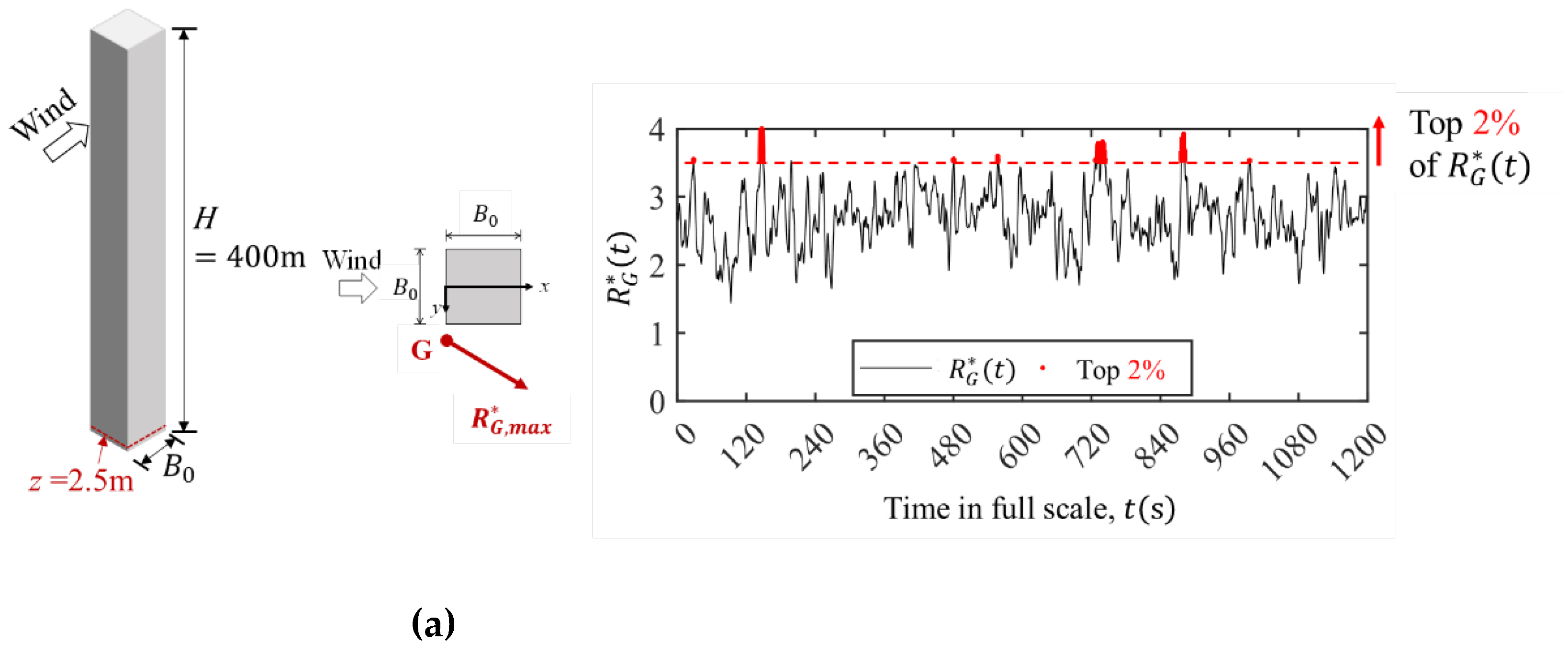
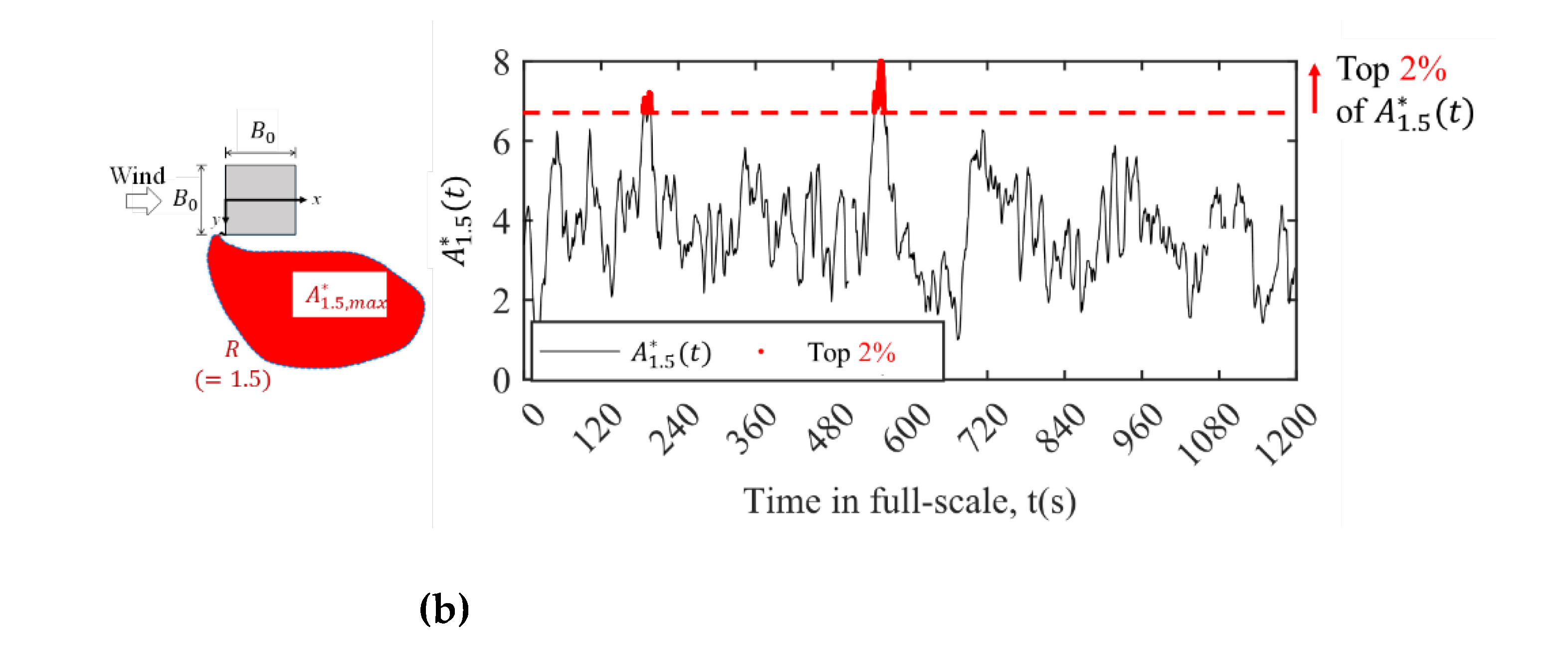
Figure 10 first shows conditional-average results for speed-up ratio vector , pressure coefficient on building surfaces and three-dimensional streamlines for the building model with aspect ratio . For the “maximum speed-up ratio” event, the area with high wind speeds (yellow to red) at pedestrian level is relatively narrow, but values of are large. Meanwhile, positive pressure on the windward surface is generally smaller and the streamlines mostly show two-dimensional characteristics.
In contrast, for the “maximum speed-up area” event, the area with high wind speeds becomes wider (yellow to red). The positive pressure on the upper part of the windward surface is quite large and the difference for the surface pressure with the lower part of windward surface and the negative pressure on the side, i.e., the pressure gradient, is also large. Accordingly, a three-dimensional flow pattern where the wind at higher level descends to near ground level is shown and a strong influence of downwash can be seen.
Figure 11 and Figure 12 further show speed-up ratio vector , pressure coefficient on building surfaces and three-dimensional streamlines for other building models with different heights or aspect ratios and . A similar phenomenon to those for the building model with aspect ratio can also be seen in the building models with different heights or aspect ratios. The difference is that the values of speed-up ratio , the positive pressure on the upper part of the windward surface and its difference with the lower part of the windward surface and the negative pressure on the side, i.e., the pressure gradients, are larger for building models with higher heights or larger aspect ratios . Meanwhile, building models tend to be slender with increase of building height or aspect ratio. The incoming flows easily pass by the sides of the building and the flow around the building tends to be two dimensional [9,26]. Therefore, the difference between conditional average results for two strong events providing “maximum speed-up ratio” and “maximum speed-up area” is more obvious at the lower part for building models with higher heights or larger aspect ratios .
Figure 13 quantitatively summarizes the conditional average results shown in Figures 10~12 for the normalized speed-up ratio at point “G”, and normalized speed-up area at pedestrian level corresponding to the two strong events providing “maximum speed-up ratio” and “maximum speed-up area”. It is obvious that compared to the situation providing “maximum speed-up area” (red color), is larger and is smaller for the situation providing “maximum speed-up ratio” (blue color). Conversely, is larger and is smaller for the situation providing “maximum speed-up area”. Meanwhile, with an increase of aspect ratio , the difference in both and between the two situations providing “maximum speed-up ratio” and “maximum speed-up area” becomes larger.
In addition, instantaneous flow patterns around all building models corresponding to the moments and , when actual maximum speed-up ratio at pedestrian-level and maximum speed-up area happen, are also checked as a reference and shown in Figure 14. Similar phenomena can be seen by comparing conditional average results in Figure 10, Figure 11 and Figure 12 and actual instantaneous results, where downwash flows at the moment for the building model with are most obvious and it may be due to relatively higher approaching flow at front stagnation level and the mediate slenderness of the building model. This also suggests the reasonableness of using the conditional average results to discuss the flow patterns corresponding to the two strong wind events.
In summary, the results above indicate that flow patterns around buildings for strong wind events providing “maximum speed-up ratio” and “maximum speed-up area” are different: the contribution of downwash tends to be larger for “maximum speed-up area” event showing more three-dimensional flow characteristics.
5. Conclusions
LES was conducted for square-section building models with different heightsin full-scale or aspect ratios , and , focusing on two instantaneous strong wind events providing “maximum speed-up ratio” and “maximum speed-up area” of pedestrian-level wind. The following findings were obtained.
Two strong wind events do not occur simultaneously.
Conditional-average flow patterns around buildings for the two instantaneous strong wind events are different: the contribution of downwash tends to be larger for the strong wind event providing “maximum speed-up area” of pedestrian-level wind, showing more three-dimensional flow characteristics.
For building models with different heights or aspect ratios , a similar phenomenon as described above can also be seen. The difference is that the values of speed-up ratio , the positive pressure on the upper part of the windward surface and its difference with the lower part of windward surface and the negative pressure on the side, i.e., the pressure gradient, are larger for building models with higher heights or larger aspect ratios .
Author Contributions
Conceptualization, Yukio Tamura; Data curation, Qiang Lin; Formal analysis, Qiang Lin and Hideyuki Tanaka; Funding acquisition, Qingshan Yang and Yukio Tamura; Investigation, Qiang Lin, Naoko Konno and Hideyuki Tanaka; Project administration, Qingshan Yang; Supervision, Qingshan Yang and Yukio Tamura; Writing – original draft, Qiang Lin and Naoko Konno; Writing – review & editing, Qiang Lin, Naoko Konno, Hideyuki Tanaka and Yukio Tamura. All authors have read and agreed to the published version of the manuscript.
Funding
This research was partially supported by 111 Project of China (B18062, B13002) and the TPU Wind Engineering Joint Usage/ Research Center Project of MEXT Japan (JPMXP0619217840). The authors are grateful for these financial supports.
Institutional Review Board Statement
Not applicable.
Informed Consent Statement
Not applicable.
Data Availability Statement
No supplementary data were produced in this research.
Acknowledgement
The authors wish to thank Prof. Akihito Yoshida from Tokyo Polytechnic University for providing support and reference on pressure coefficients for a square-section building model in TPU aerodynamic database.
Conflicts of Interest
The authors declare no conflict of interest.
Appendix A Data Acquisition Period for Conditional-Average Analysis
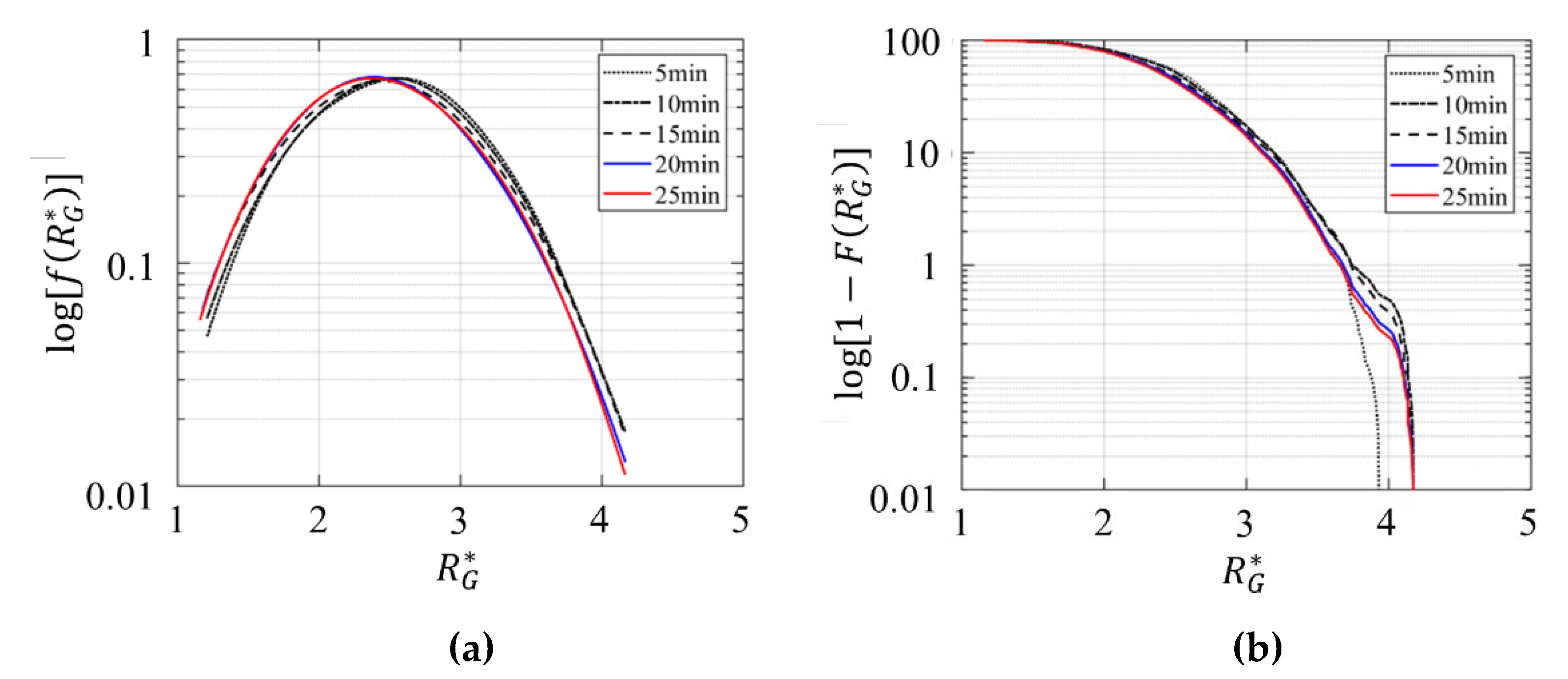
The probability density functions (PDFs) of the and are denoted as and , and corresponding cumulative distribution functions (CDFs) are denoted as and .
Figure A1 and Figure A2 compare PDFs and CDFs over various data acquisition periods (5~25min in full scale) for and , respectively. It can be seen that the differences between PDFs and CDFs at 20min and 25min are negligible (blue and red solid lines). This may indicate that the data acquisition period of 20min in full scale is sufficient to ensure acceptable uncertainty.
Figure A1.
Comparison of (a) probability density function
and (b) cumulative distribution function of the instantaneous wind speed ratio over various data acquisition periods (5~25min in full scale).
Figure A2.
Comparison of (a) probability density function
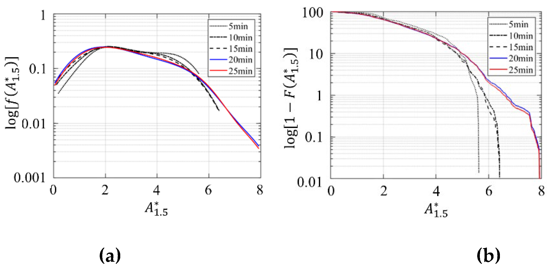
and (b) cumulative distribution function of the instantaneous speed-up area over various data acquisition periods (5~25min in full scale).
References
- Lawson, T.V.; Penwarden, A.D. The Effect of Wind on People in the Vicinity of Buildings. In Proceedings of the In: Proceedings 4th International Conference on Wind Effects on Buildings and Structures; Cambridge University Press; 1975; pp. 605–622. [Google Scholar]
- Wise, A.F.E. Effects Due to Groups of Buildings. Philosophical Transactions of the Royal Society of London. Series A, Mathematical and Physical Sciences 1971, 269, 469–485. [Google Scholar] [CrossRef]
- Hunt, J.C.R.; Poulton, E.C.; Mumford, J.C. The Effects of Wind on People; New Criteria Based on Wind Tunnel Experiments. Building and Environment 1976, 11, 15–28. [Google Scholar] [CrossRef]
- Murakami, S.; Deguchi, K. New Criteria for Wind Effects on Pedestrians. Journal of Wind Engineering and Industrial Aerodynamics 1981, 7, 289–309. [Google Scholar] [CrossRef]
- Vita, G.; Shu, Z.; Jesson, M.; Quinn, A.; Hemida, H.; Sterling, M.; Baker, C. On the Assessment of Pedestrian Distress in Urban Winds. Journal of Wind Engineering and Industrial Aerodynamics 2020, 203, 104200. [Google Scholar] [CrossRef]
- Blocken, B.; Moonen, P.; Stathopoulos, T.; Carmeliet, J. Numerical Study on the Existence of the Venturi Effect in Passages between Perpendicular Buildings. J. Eng. Mech. 2008, 134, 1021–1028. [Google Scholar] [CrossRef]
- Dutt, A.J. Wind Flow in an Urban Environment. Environ. Monit. Assess. 1991, 19, 495–506. [Google Scholar] [CrossRef]
- Gandemer, J. Discomfort Due to Wind near Buildings: Aerodynamic Concepts. National Institute of Standards and Technology 1978. [CrossRef]
- Tamura, Y.; Xu, X.D.; Yang, Q.S. Characteristics of Pedestrian-Level Mean Wind Speed around Square Buildings: Effects of Height, Width, Size and Approaching Flow Profile. J. Wind Eng. Ind. Aerodyn. 2019, 192, 74–87. [Google Scholar] [CrossRef]
- Yang, Q.; Xu, X.; Lin, Q.; Tamura, Y. Generic Models for Predicting Pedestrian-Level Wind around Isolated Square-Section High-Rise Buildings. Journal of Wind Engineering and Industrial Aerodynamics 2022, 220, 104842. [Google Scholar] [CrossRef]
- COOK, N.J. The Designer’s Guide to Wind Loading of Building Structures. I. Background, Damage Survey, Wind Data and Structural Classification; Building Research Establishment report; Butterworths: London, 1985; ISBN 978-0-408-00870-9. [Google Scholar]
- Blocken, B.; Carmeliet, J. Pedestrian Wind Environment around Buildings: Literature Review and Practical Examples. Journal of Thermal Envelope and Building Science 2004, 28, 107–159. [Google Scholar] [CrossRef]
- Beranek, W.J. Wind Environment around Single Buildings of Rectangular Shape. Heron 1984, 29, 1–31. [Google Scholar]
- Sexton, D. 1967.
- Franke, J.; Hellsten, A.; Schlunzen, K.H.; Carissimo, B. The COST 732 Best Practice Guideline for CFD Simulation of Flows in the Urban Environment: A Summary. IJEP 2011, 44, 419. [Google Scholar] [CrossRef]
- Tominaga, Y.; Mochida, A.; Yoshie, R.; Kataoka, H.; Nozu, T.; Yoshikawa, M.; Shirasawa, T. AIJ Guidelines for Practical Applications of CFD to Pedestrian Wind Environment around Buildings. Journal of Wind Engineering and Industrial Aerodynamics 2008, 96, 1749–1761. [Google Scholar] [CrossRef]
- Lin, Q.; Ishida, Y.; Tanaka, H.; Mochida, A.; Yang, Q.; Tamura, Y. Large Eddy Simulations of Strong Wind Mechanisms at Pedestrian Level around Square-Section Buildings with Same Aspect Ratios and Different Sizes. Building and Environment 2023, 243, 110680. [Google Scholar] [CrossRef]
- Okaze, T.; Mochida, A. Cholesky Decomposition–Based Generation of Artificial Inflow Turbulence Including Scalar Fluctuation. Computers & Fluids 2017, 159, 23–32. [Google Scholar] [CrossRef]
- TPU Aerodynamic Database Available online: https://wind.arch.t-kougei.ac.jp/system/eng/contents/code/tpu.
- Ikegaya, N.; Ikeda, Y.; Hagishima, A.; Tanimoto, J. Evaluation of Rare Velocity at a Pedestrian Level Due to Turbulence in a Neutrally Stable Shear Flow over Simplified Urban Arrays. J. Wind Eng. Ind. Aerodyn. 2017, 171, 137–147. [Google Scholar] [CrossRef]
- Kawaminami, T.; Ikegaya, N.; Hagishima, A.; Tanimoto, J. Velocity and Scalar Concentrations with Low Occurrence Frequencies within Urban Canopy Regions in a Neutrally Stable Shear Flow over Simplified Urban Arrays. J. Wind Eng. Ind. Aerodyn. 2018, 182, 286–294. [Google Scholar] [CrossRef]
- Wang, W.; Okaze, T. Statistical Analysis of Low-Occurrence Strong Wind Speeds at the Pedestrian Level around a Simplified Building Based on the Weibull Distribution. Building and Environment 2022, 209, 108644. [Google Scholar] [CrossRef]
- Du, Y.; Mak, C.M.; Kwok, K.; Tse, K.-T.; Lee, T.; Ai, Z.; Liu, J.; Niu, J. New Criteria for Assessing Low Wind Environment at Pedestrian Level in Hong Kong. Building and Environment 2017, 123, 23–36. [Google Scholar] [CrossRef]
- Lawson, T.V. The Widn Content of the Built Environment. Journal of Wind Engineering and Industrial Aerodynamics 1978, 3, 93–105. [Google Scholar] [CrossRef]
- Murakami, S.; Iwasa, Y.; Morikawa, Y. Study on Acceptable Criteria for Assessing Wind Environment at Ground Level Based on Residents’ Diaries. Journal of Wind Engineering and Industrial Aerodynamics 1986, 24, 1–18. [Google Scholar] [CrossRef]
- Tanaka, H.; Lin, Q.; Azegami, Y.; Tamura, Y. Verification of Speed-up Mechanism of Pedestrian-Level Winds Around Square Buildings by CFD. International Journal of High-Rise Buildings 2022, 11, 301–314. [Google Scholar] [CrossRef]
Figure 1.
Approaching flow conditions by LES. (a) Computational domain (cross section corresponds to the wind tunnel section of the PIV test in Lin et al. [17]); (b) Approaching flow profiles at inlet boundary and origin “O”.
Figure 1.
Approaching flow conditions by LES. (a) Computational domain (cross section corresponds to the wind tunnel section of the PIV test in Lin et al. [17]); (b) Approaching flow profiles at inlet boundary and origin “O”.
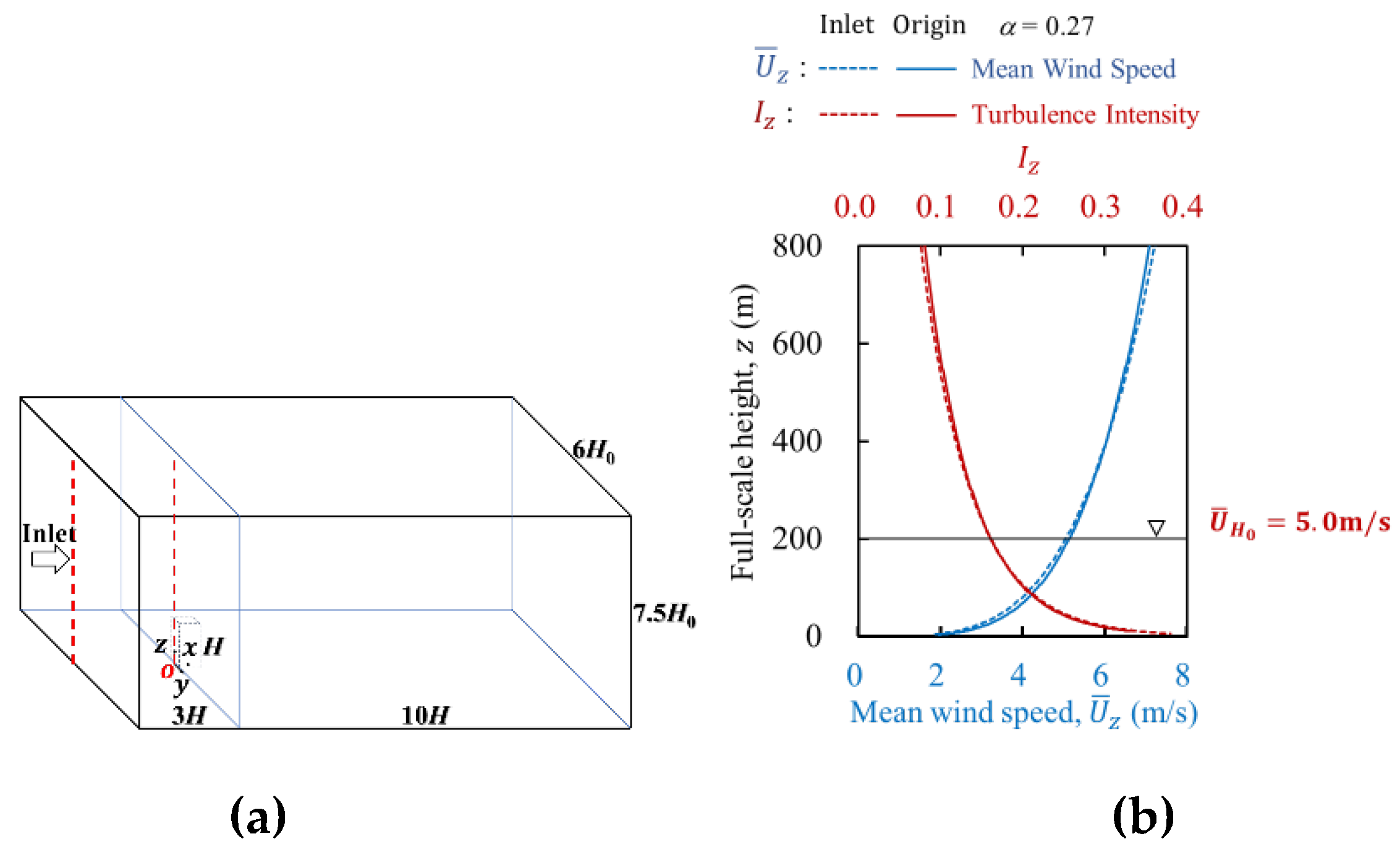
Figure 2.
Approaching flow conditions by experiment (TPU Database) and LES. (a) Computational domain (cross section corresponds to the TPU wind tunnel section); (b) Approaching flow profile; (c) Power spectrum at height of building top, z = Hd = 200m.
Figure 2.
Approaching flow conditions by experiment (TPU Database) and LES. (a) Computational domain (cross section corresponds to the TPU wind tunnel section); (b) Approaching flow profile; (c) Power spectrum at height of building top, z = Hd = 200m.
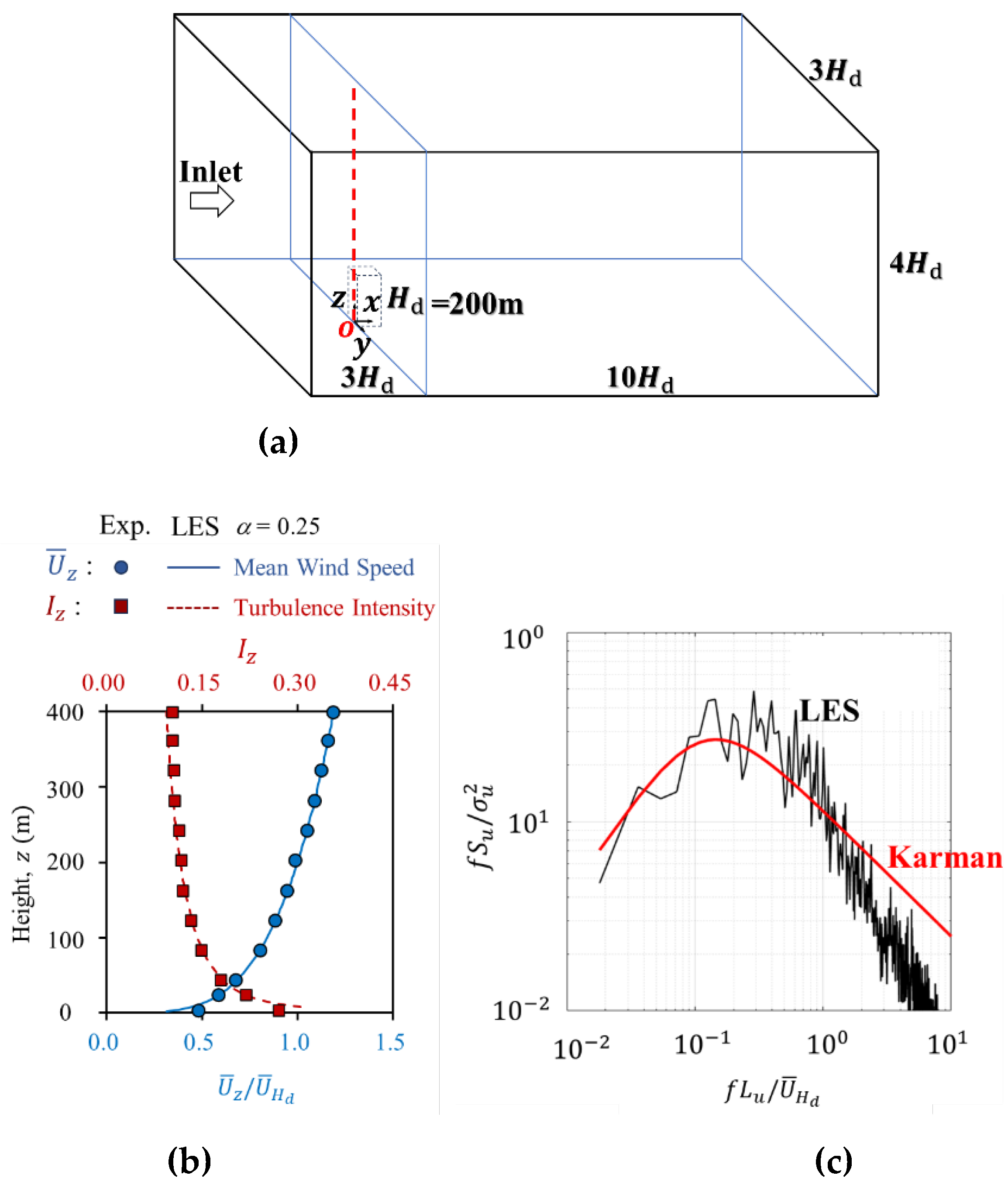
Figure 3.
Wind pressure coefficients around the perimeter of a building at z = 2Hd/3. (a) Mean Cp,d; (b) Fluctuating Cp,d.
Figure 3.
Wind pressure coefficients around the perimeter of a building at z = 2Hd/3. (a) Mean Cp,d; (b) Fluctuating Cp,d.
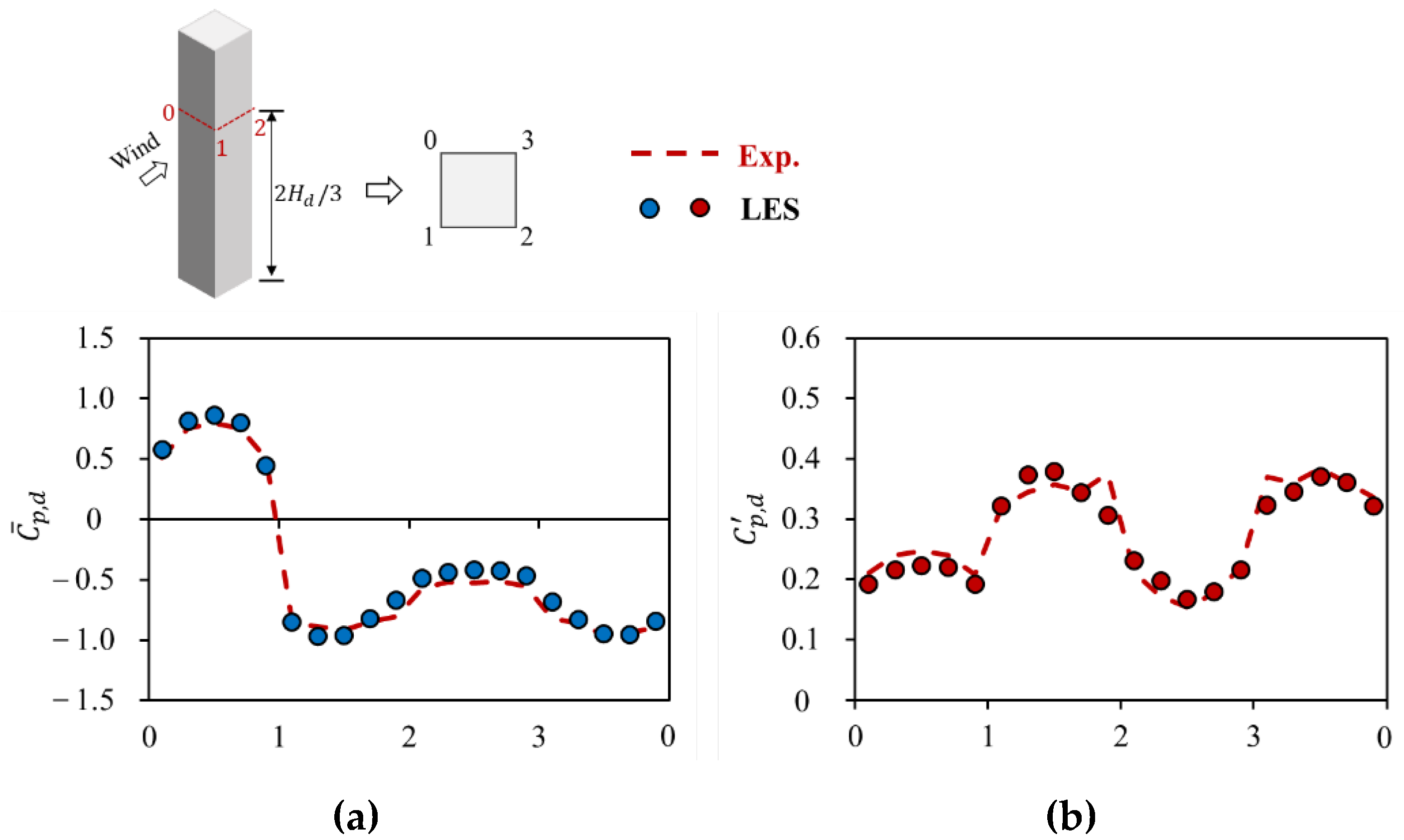
Figure 4.
Comparison of wind pressure coefficients for all the pressure monitoring taps on building surfaces from LES and experimental results. (a) Mean Cp,d; (b) Fluctuating Cp,d.
Figure 4.
Comparison of wind pressure coefficients for all the pressure monitoring taps on building surfaces from LES and experimental results. (a) Mean Cp,d; (b) Fluctuating Cp,d.
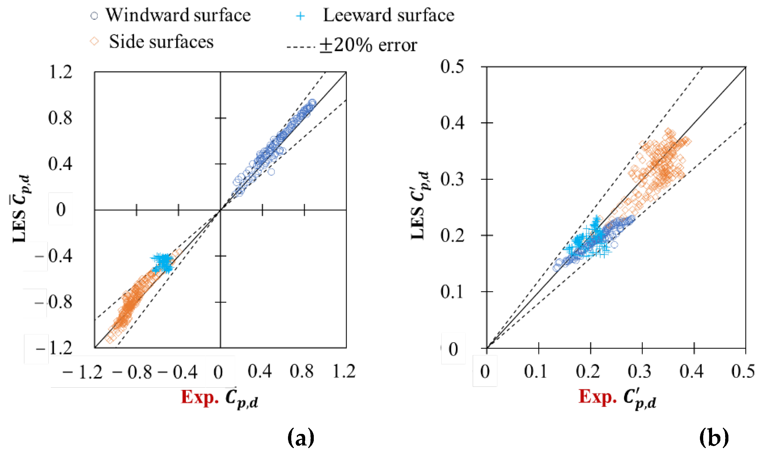
Figure 5.
Comparison of contours of wind pressure coefficients on building surfaces from LES and experimental results. (a) Mean Cp,d; (b) Fluctuating Cp,d.
Figure 5.
Comparison of contours of wind pressure coefficients on building surfaces from LES and experimental results. (a) Mean Cp,d; (b) Fluctuating Cp,d.
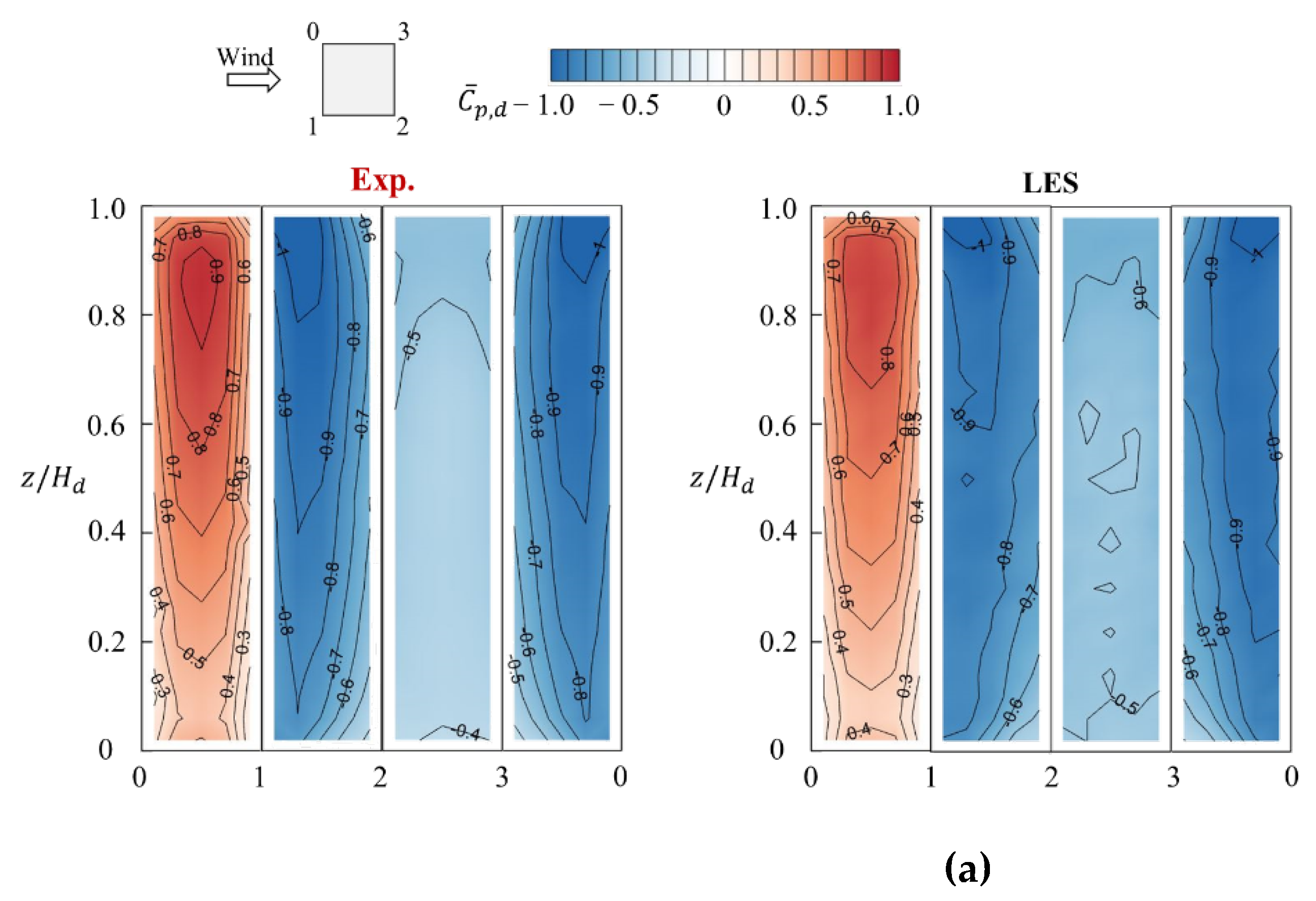
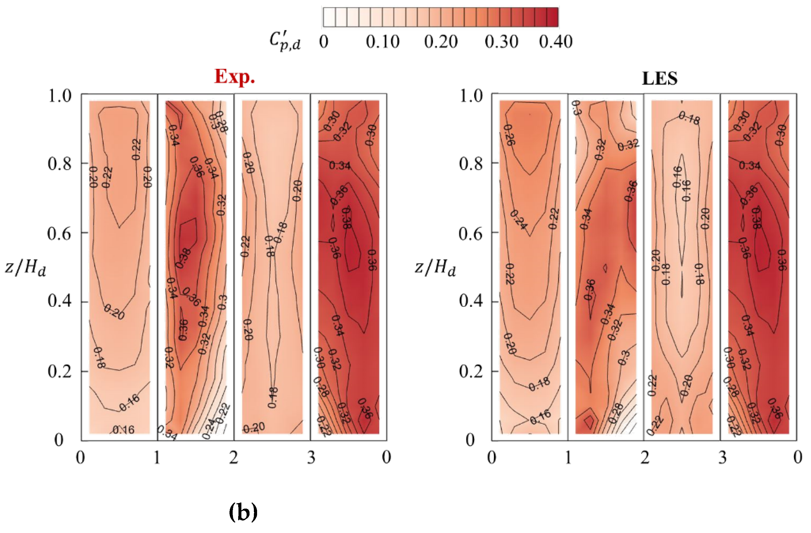
Figure 6.
Definition of (a) Point “G” and (b) normalized instantaneous speed-up area, .
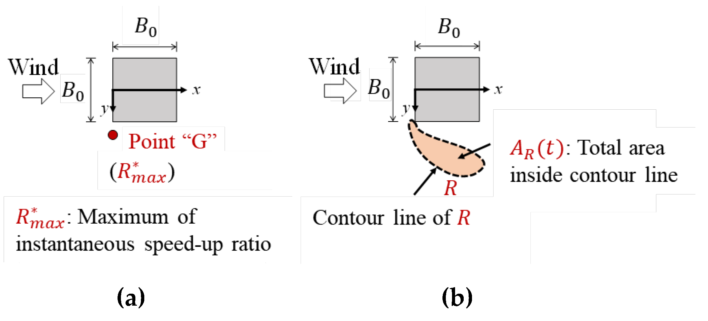
Figure 7.
Extraction of maximum-level of speed-up ratio and normalized speed-up area at pedestrian level around the building model with aspect ratio 2. (a) “Maximum speed-up ratio” event, ; (b) “Maximum speed-up area” event
Figure 7.
Extraction of maximum-level of speed-up ratio and normalized speed-up area at pedestrian level around the building model with aspect ratio 2. (a) “Maximum speed-up ratio” event, ; (b) “Maximum speed-up area” event
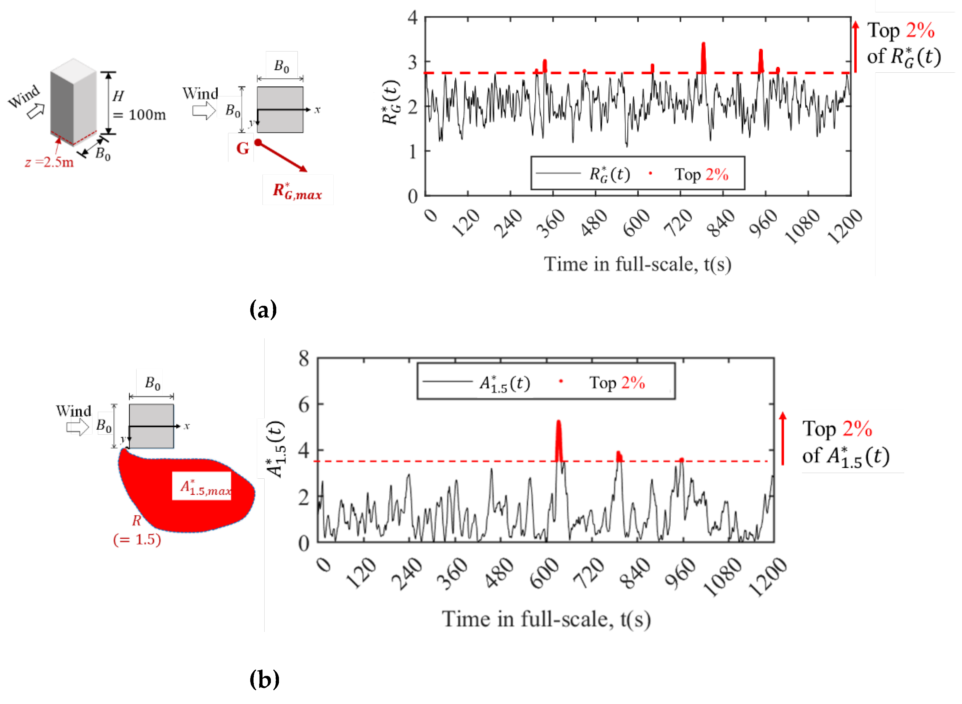
Figure 8.
Extraction of maximum-level of speed-up ratio and normalized speed-up area at pedestrian level around the building model with aspect ratio . (a) “Maximum speed-up ratio” event, ; (b) “Maximum speed-up area” event
Figure 8.
Extraction of maximum-level of speed-up ratio and normalized speed-up area at pedestrian level around the building model with aspect ratio . (a) “Maximum speed-up ratio” event, ; (b) “Maximum speed-up area” event
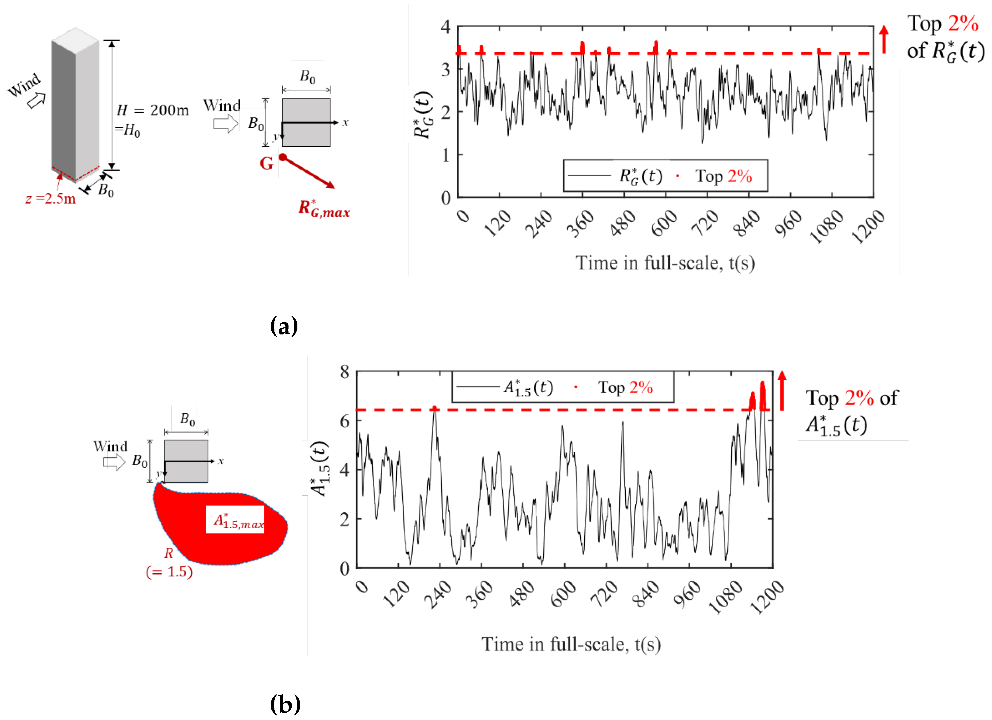
Figure 10.
Conditional-averaged results for strong wind events providing “maximum speed-up ratio” (left) and “maximum speed-up area” (right) for building model with aspect ratio . (a) Conditional-averaged speed-up ratio vector and pressure coefficient on building surfaces; (b) Conditional-averaged streamlines with speed-up ratio.
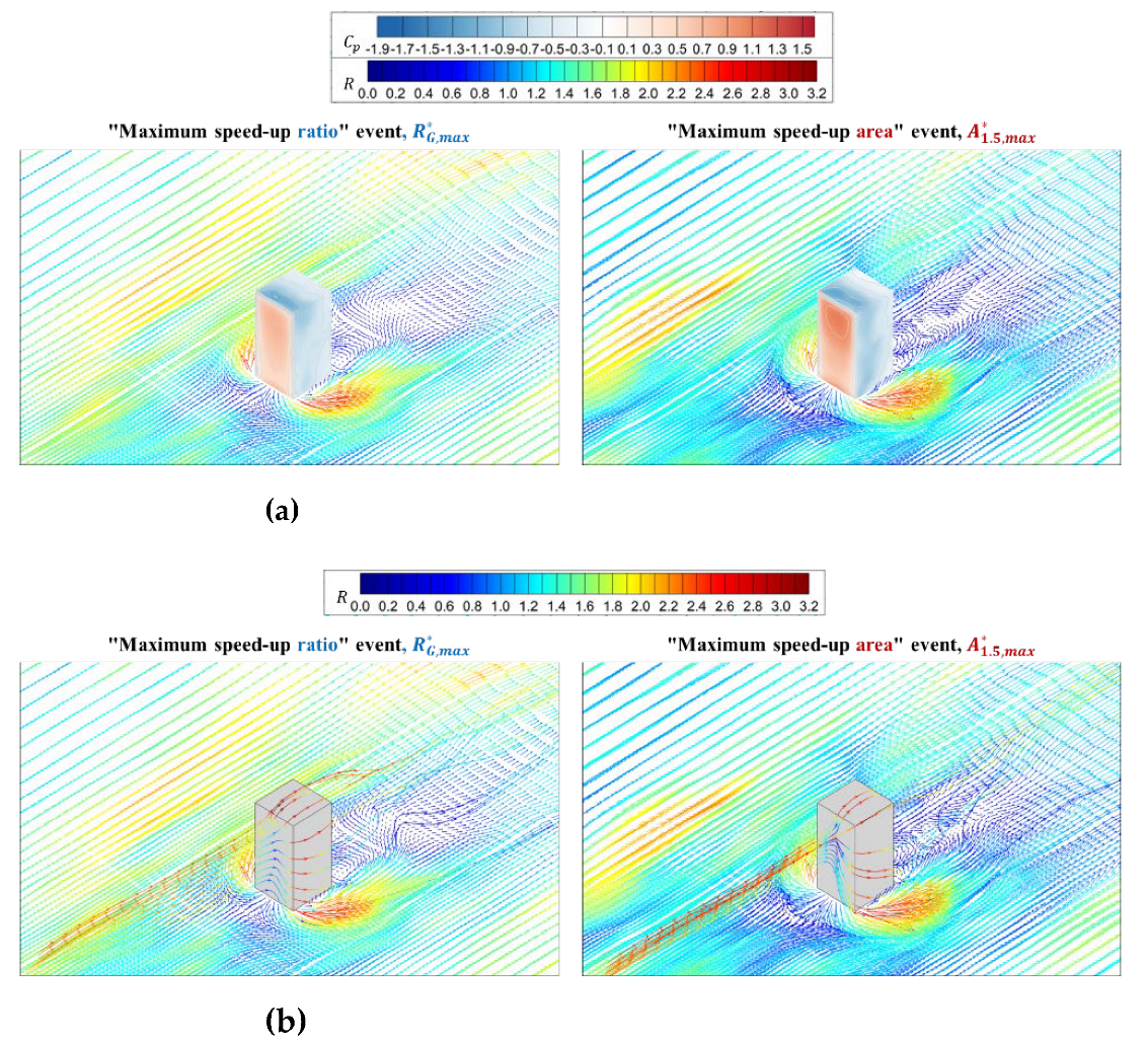
Figure 11.
Conditional-averaged results for strong wind events providing “maximum speed-up ratio” (left) and “maximum speed-up area” (right) for building model with aspect ratio . (a) Conditional-averaged speed-up ratio vector and pressure coefficient on building surfaces; (b) Conditional-averaged streamlines with speed-up ratio.
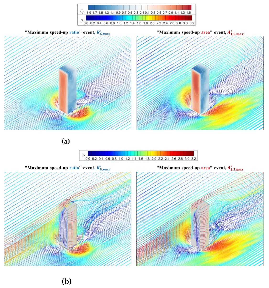
Figure 12.
Conditional-averaged results for strong wind events providing “maximum speed-up ratio” (left) and “maximum speed-up area” (right) for building model with aspect ratio . (a) Conditional-averaged speed-up ratio vector and pressure coefficient on building surfaces; (b) Conditional-averaged streamlines with speed-up ratio.
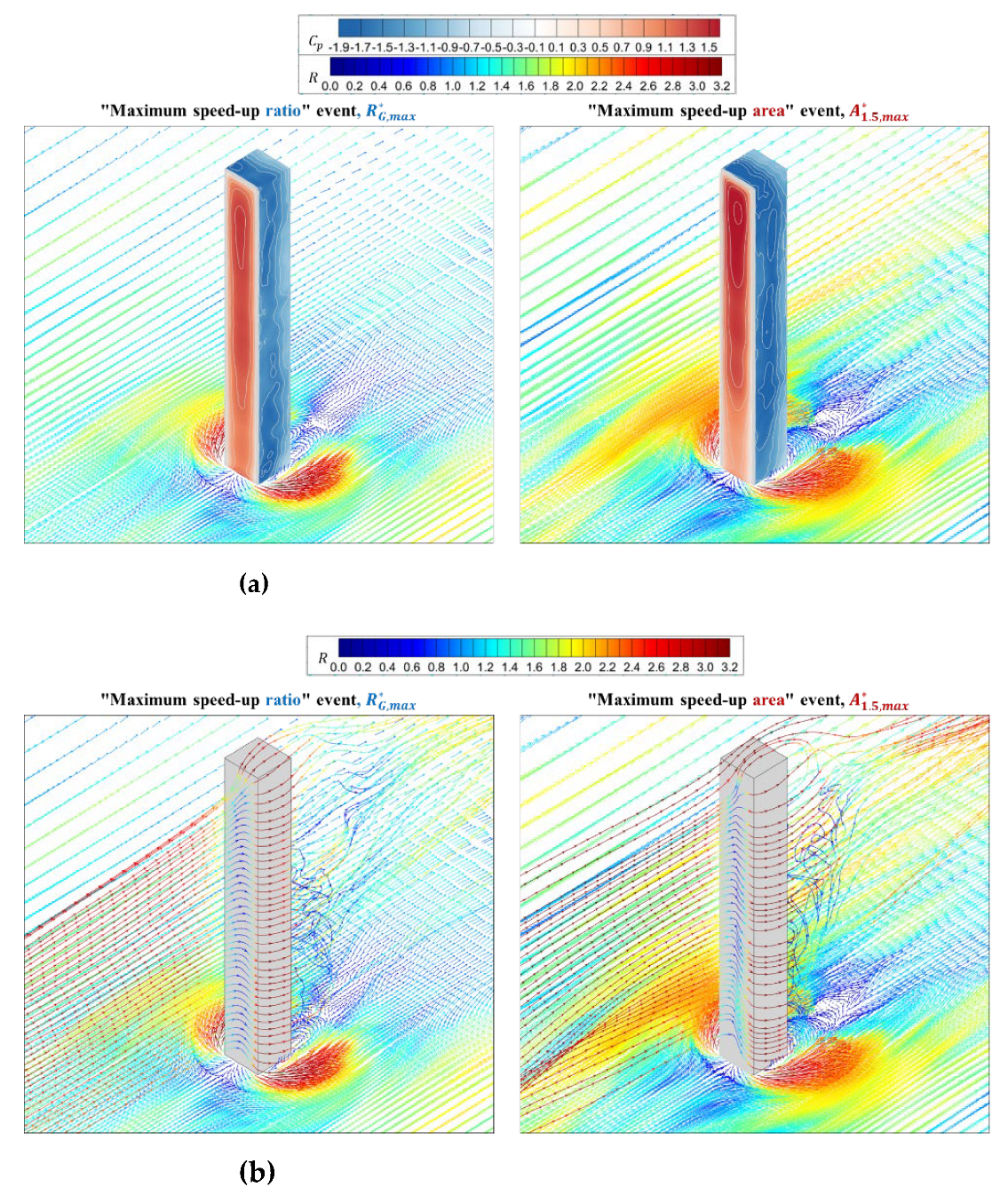
Figure 13.
Conditional average results for normalized speed-up ratio at point “G”, and normalized speed-up area at pedestrian level corresponding to the two strong events providing “maximum speed-up ratio” and “maximum speed-up area” (a) Conditional-averaged ; (b) Conditional-averaged
Figure 13.
Conditional average results for normalized speed-up ratio at point “G”, and normalized speed-up area at pedestrian level corresponding to the two strong events providing “maximum speed-up ratio” and “maximum speed-up area” (a) Conditional-averaged ; (b) Conditional-averaged
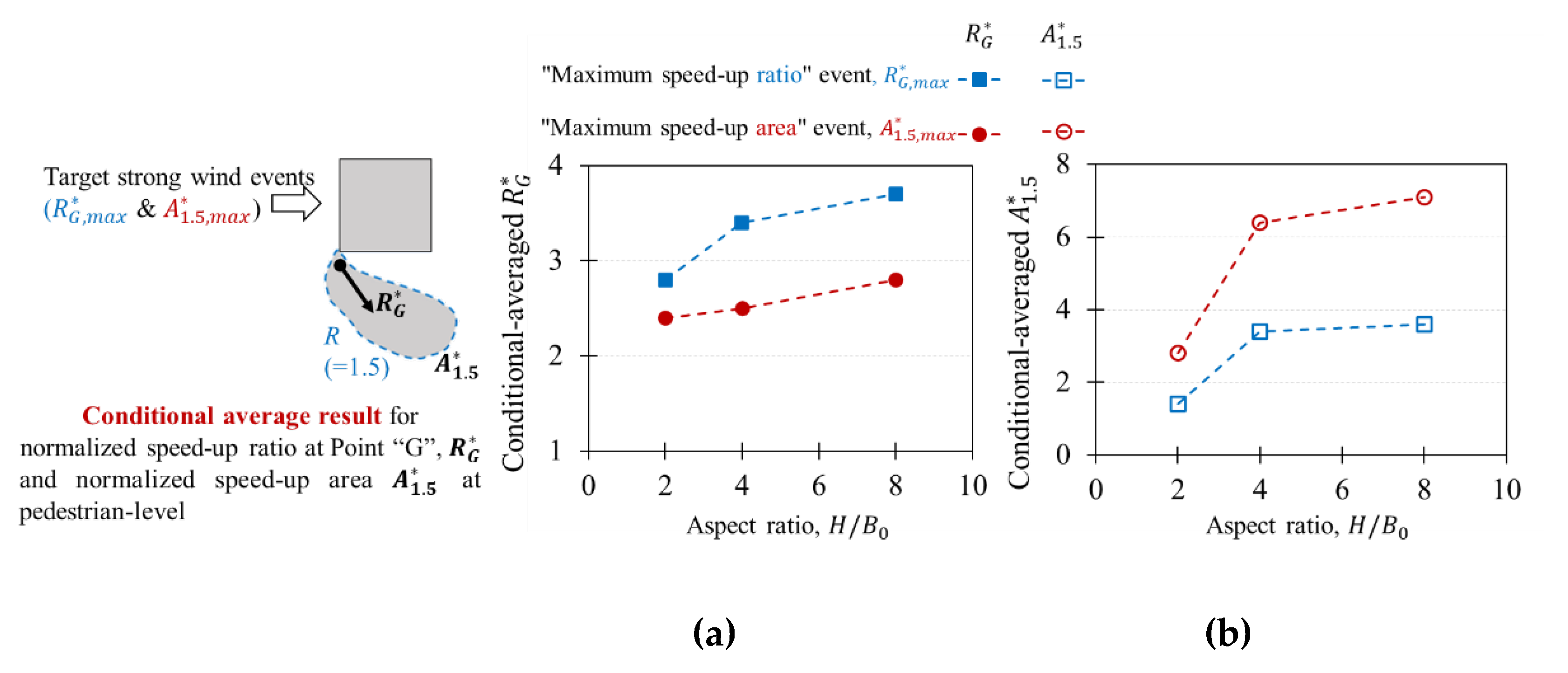
Figure 14.
Instantaneous streamlines with speed-up ratio and pressure coefficient on building surfaces when actual maximum speed-up ratio at pedestrian-level, and maximum speed-up area, happen for building model with aspect ratios and 8. (a) Height, or aspect ratio 2; (b) Height, or aspect ratio 4; (c) Height, or aspect ratio 8.
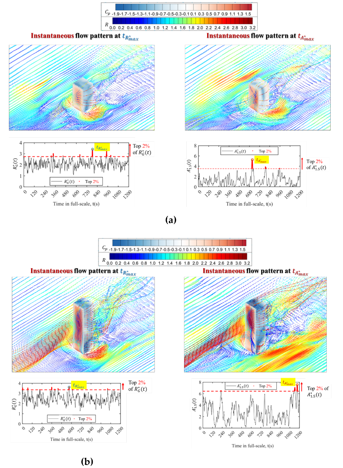
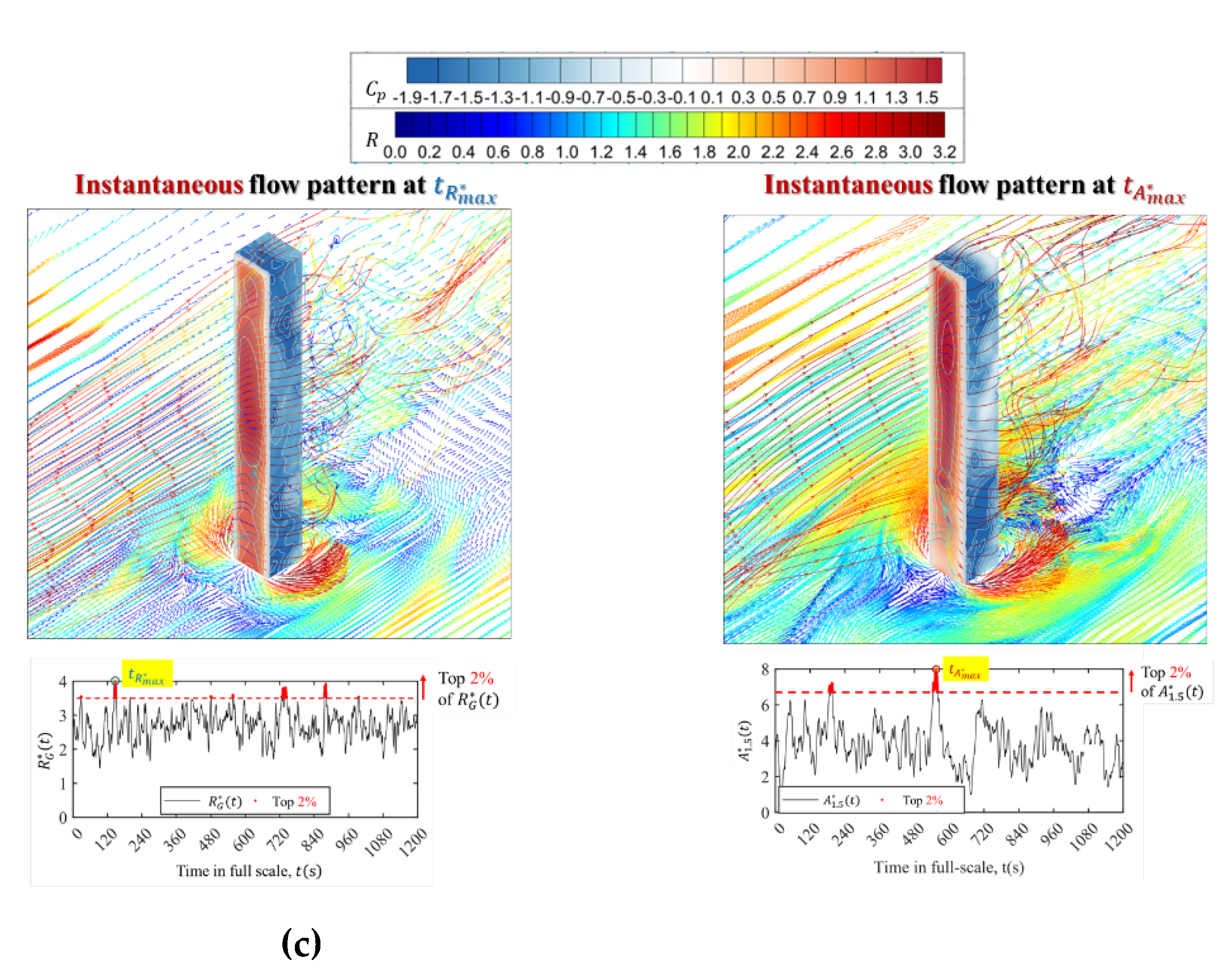

Table 1.
Model configurations.
| Width, B (m) | (Constant) | ||
| Height, H (m) | 100 | 400 | |
| Aspect ratio, | 2 | 4 | 8 |
 |
 |
 |
 |
 |
 |
 |
|
Table 2.
Calculation conditions for LES.
| Code | OpenFOAM v8 |
|---|---|
| Computational domain | |
| SGS model | WALE model |
| Time scheme | Second-order backward |
| Time interval for time advancement | 1×10⁻⁴ s |
| Advection scheme | Second-order central difference (95%)+ First-order upwind difference (5%) |
| Diffusion scheme | Second-order linear difference |
| Pressure solver | PISO |
| Inflow fluctuation | Artificial generation method [18] |
| Outlet boundary | Advective outflow condition |
| Upper & side boundaries | No-slip wall |
| Ground & building boundaries | Spalding’s law |
Disclaimer/Publisher’s Note: The statements, opinions and data contained in all publications are solely those of the individual author(s) and contributor(s) and not of MDPI and/or the editor(s). MDPI and/or the editor(s) disclaim responsibility for any injury to people or property resulting from any ideas, methods, instructions or products referred to in the content. |
© 2025 by the authors. Licensee MDPI, Basel, Switzerland. This article is an open access article distributed under the terms and conditions of the Creative Commons Attribution (CC BY) license (http://creativecommons.org/licenses/by/4.0/).
Copyright: This open access article is published under a Creative Commons CC BY 4.0 license, which permit the free download, distribution, and reuse, provided that the author and preprint are cited in any reuse.


