The General Solution to a System of Tensor Equations over the Split Quaternion Algebra with Applications

1. Introduction

In 1843, William Rowan Hamilton introduced the concept of real quaternions [1] defined by

$$\mathbb{H}=\{q=q_0+q_{1}i+q_{2}j+q_{3}k:i^2=j^2=k^2=-1,ijk=-1,q_0,q_1,q_2,q_3\in \mathbb{R}\},$$

where $\mathbb{H}$ and $\mathbb{R}$ separately denoted the set of real quaternions and the set of real numbers. Quaternions have been utilized in numerous areas, including the analysis of quaternion random signals [2], color image processing [3,4] and face recognition [5]. As theory of quaternion evolved, James Cockle introduced the concept of split quaternions [6] in 1849:

$${\mathbb{Q}}_S=\{q=q_0+q_{1}i+q_{2}j+q_{3}k:q_0,q_1,q_2,q_3\in \mathbb{R}\},$$

where the imaginary identities $i,j,k$ satisfied

$$i^2=-1,j^2=k^2=1,ijk=1,$$

$$ij=-ji=k,jk=-kj=-i,ki=-ik=j.$$

Split quaternions have diverse applications across various fields. In physics, they are used to model spacetime symmetries and rotations in relativity [7]. In computer graphics, split quaternions assist in efficiently handling 3D rotations and transformations [8]. Split quaternions also have applications in control theory, signal processing, and robotics, where they help in representing and solving complex spatial relationships and transformations [9].

Tensors, as mathematical constructs that generalize scalars, vectors, and matrices to higher dimensions, are extensively applied across a wide range of scientific and engineering domains due to their capability to manage complex data structures. In computer vision and image processing, tensors are used to represent multi-dimensional image data, with convolution operations in neural networks being performed as tensor operations [10]. In physics, tensors are fundamental in general relativity for describing spacetime geometry [11] and in electromagnetism for unifying electric and magnetic fields [12]. In machine learning, tensors are core data structures in frameworks like TensorFlow and PyTorch, playing a crucial role in optimization and model training [13,14]. They are also essential in data analysis for dimensionality reduction and feature extraction, particularly within recommendation systems [15]. The multi-dimensional nature of tensors makes them powerful tools for handling complex data, and their significance continues to grow with advancements in computational power and algorithms.

$\mathcal{A}=\left(a_{i_1\cdots i_N}\right)(1\le i_j\le I_j,j=1,...,N)$ presents an N-dimensional tensor, which is a natural extension of the matrix. For N = 1, $\mathcal{A}$ is a vector. For N = 2, $\mathcal{A}$ is a matrix. In recent decades, numerous researchers have made significant contributions to the study of tensors and quaternions. For example, Qi et al. [16,17,18] researched the spectral theory of tensor and tensor eigenvalues. Wang et al. [19,20,21] examined systems of tensor equations within the framework of quaternion algebra. Chen et al. [22,23] derived some solvability conditions and formulated expressions of the general $\eta$-(anti)-Hermitian solution to constrained Sylvester-type matrix equations over the generalized commutative quaternion algebra ${\mathbb{S}}_g$. Gao et al. [24] established the necessary and sufficient conditions for the existence of (anti-)$\eta$-Hermitian solutions to a system of matrix equations over split quaternion algebra. Xie et al. [25] proposed the BiCG algorithm for solving the minimal Frobenius norm solution of generalized Sylvester tensor equation over the quaternions. Yang et al. [26] researched a system of tensor equations over the dual split quaternion algebra with an application.

To the best of our knowledge, there is relatively little research on tensor equations over split quaternions at present. Motivated by the aforementioned research and the existing applications of tensor equation systems over split quaternion algebra, we aim to study the solvability conditions and find the general solution for the following system of split quaternion tensor equations

$$\left\{\begin{array}{c}{\mathcal{A}}_1{\ast }_N{\mathcal{X}}_1={\mathcal{P}}_1,\hfill \\ {\mathcal{X}}_1{\ast }_N{\mathcal{B}}_1={\mathcal{Q}}_1,\hfill \\ {\mathcal{A}}_2{\ast }_N{\mathcal{X}}_2={\mathcal{P}}_2,\hfill \\ {\mathcal{X}}_2{\ast }_N{\mathcal{B}}_2={\mathcal{Q}}_2,\hfill \\ \cdots \hfill \\ {\mathcal{A}}_n{\ast }_N{\mathcal{X}}_n={\mathcal{P}}_n,\hfill \\ {\mathcal{X}}_n{\ast }_N{\mathcal{B}}_n={\mathcal{Q}}_n,\hfill \\ \sum _{t=1}^n{\mathcal{E}}_t{\ast }_N{\mathcal{X}}_t{\ast }_N{\mathcal{F}}_t=\mathcal{H},\hfill \end{array}\right.$$

(1)

where ${\mathcal{A}}_t,{\mathcal{P}}_t,{\mathcal{B}}_t,{\mathcal{Q}}_t,{\mathcal{E}}_t,{\mathcal{F}}_t(t=1,...,n)$ and $\mathcal{H}$ are given quaternion tensors and ${\mathcal{X}}_t(t=1,...,n)$ are unknown split quaternion tensors.

This paper is organized as follows: In Section 2, some basic theories and relevant properties of quaternion tensors are reviewed. In Section 3, we derive some practical necessary and sufficient conditions for the existence of the general solution to the system (1) over ${\mathbb{Q}}_S$. Furthermore, the formula of the general solution to the system (1) is also given when it is solvable. Especially, the unique solution is given when the uniqueness condition is satisfied. In Section 4, two algorithms and one numerical example are given in order to illustrate our results. In Section 5, we provide four algorithms and two examples for color videos encryption and decryption. In Section 6, we make a conclusion to summarize this paper.

In subsequent chapters, the symbols ${\mathbb{R}}^{m\times n}$, ${\mathbb{C}}^{m\times n}$, ${\mathbb{Q}}_S^n$, ${\mathbb{Q}}_S^{m\times n}$ are used to represent the set of all $m\times n$ real matrices, all $m\times n$ complex matrices, all n dimensional split quaternion column vectors and all $m\times n$ split quaternion matrices. The symbol $r\left(A\right)$ denotes the rank of the matrix A. Denote I as the identity matrix and O as the zero matrix with an appropriate size. $\overline{A},A^T,A^{\ast },A^{†}$ denote the conjugate, the transpose, the conjugate transpose and the Moore-Penrose inverse of the matrix A, repectively. Let ${\mathbb{R}}^{I_1\times \cdots \times I_N\times J_1\times \cdots \times J_N},{\mathbb{C}}^{I_1\times \cdots \times I_N\times J_1\times \cdots \times J_N},$ and ${\mathbb{Q}}_S^{I_1\times \cdots \times I_N\times J_1\times \cdots \times J_N}$ represent the set of all corresponding dimensional real tensors, complex tensors, and split quaternion tensors, respectively.

2. Preliminaries

This chapter primarily introduces split quaternion tensors, the Einstein product of split quaternion tensors, the complex representation and related properties of split quaternion matrices and so on. These concepts lay the groundwork for deriving the main conclusions presented in the subsequent chapter.

Definition 1.

 [27] For two split quaternion tensors $\mathcal{A}=\left(a_{i_1\cdots i_N{j}_1\cdots j_L}\right)\in {\mathbb{Q}}_S^{I_1\times \cdots \times I_N\times J_1\times \cdots \times J_L}$ and $\mathcal{B}=\left(b_{j_1\cdots j_L{k}_1\cdots k_M}\right)\in {\mathbb{Q}}_S^{J_1\times \cdots \times J_L\times K_1\times \cdots \times K_M}$, the Einstein product of $\mathcal{A}$ and $\mathcal{B}$ is defined by the operation ${\ast }_L$ via

$${\left(\mathcal{A}{\ast }_L\mathcal{B}\right)}_{i_1\cdots i_N{k}_1\cdots k_M}=\sum _{j_1\cdots j_L}{a}_{i_1\cdots i_N{j}_1\cdots j_L}{b}_{j_1\cdots j_L{k}_1\cdots k_M},$$

where $\mathcal{A}{\ast }_L\mathcal{B}\in {\mathbb{Q}}_S^{I_1\times \cdots \times I_N\times K_1\times \cdots \times K_M}$.

The Einstein product of tensors is closely related to matrix multiplication. We introduce a mapping that establishes an isomorphic relationship between tensors with respect to the Einstein product and matrices with respect to the general matrix product.

Definition 2.

 [28] There exists an isomorphic mapping f from ${\mathbb{Q}}_S^{I_1\times \cdots \times I_N\times J_1\times \cdots \times J_N}$ to ${\mathbb{Q}}_S^{I\times J}$ denoted as

$$\begin{array}{ccc}\hfill f:{\mathbb{Q}}_S^{I_1\times \cdots \times I_N\times J_1\times \cdots \times J_N}& \to & {\mathbb{Q}}_S^{I\times J}\hfill \\ \hfill a_{i_1\cdots i_N{j}_1\cdots j_N}& \mapsto & a_{[i_N+{\sum }_{K=1}^{N-1}(i_K-1){\prod }_{S=K+1}^N{I}_S][j_N+{\sum }_{K=1}^{N-1}\left[(j_K-1){\prod }_{S=K+1}^N{J}_S\right]},\hfill \end{array}$$

where $I=I_1\cdots I_N$ and $J=J_1\cdots J_N$.

It is apparent that f is a one-to-one mapping. Therefore, the inverse mapping $f^{-1}:{\mathbb{Q}}_S^{I\times J}\to {\mathbb{Q}}_S^{I_1\times \cdots \times I_N\times J_1\times \cdots \times J_N}$ exists. Subsequently, we prove that f is an isomorphic mapping.

Proof. 

For $\mathcal{A}=\left(a_{i_1\cdots i_N{j}_1\cdots j_L}\right)\in {\mathbb{Q}}_S^{I_1\times \cdots \times I_N\times J_1\times \cdots \times J_L}$ and $\mathcal{B}=\left(b_{j_1\cdots j_L{k}_1\cdots k_M}\right)\in {\mathbb{Q}}_S^{J_1\times \cdots \times J_L\times K_1\times \cdots \times K_M}$, we need to prove $f\left(\mathcal{A}{\ast }_L\mathcal{B}\right)=f\left(\mathcal{A}\right)·f\left(\mathcal{B}\right)$, where ${\ast }_L$ and · denote the Einstein product and matrix product, respectively.

Through the definition of the Einstein product, then

$${\left(\mathcal{A}{\ast }_L\mathcal{B}\right)}_{i_1\cdots i_N{k}_1\cdots k_M}=\sum _{j_1\cdots j_L}{a}_{i_1\cdots i_N{j}_1\cdots j_L}{b}_{j_1\cdots j_L{k}_1\cdots k_M}.$$

By direct computation, we obtain

$$\begin{array}{ccc}\hfill f\left(\mathcal{A}{\ast }_L\mathcal{B}\right)& =& f\left(\sum _{j_1\cdots j_L}{a}_{i_1\cdots i_N{j}_1\cdots j_L}{b}_{j_1\cdots j_L{k}_1\cdots k_M}\right)\hfill \\ & =& \sum _{j_1\cdots j_L}{a}_{[i_N+{\sum }_{K=1}^{N-1}(i_K-1){\prod }_{S=K+1}^N{i}_S][j_L+{\sum }_{K=1}^{L-1}\left[(j_K-1){\prod }_{S=K+1}^L{j}_S\right]}\hfill \\ & & b_{[j_L+{\sum }_{K=1}^{L-1}\left[(j_K-1){\prod }_{S=K+1}^L{j}_S\right][k_M+{\sum }_{K=1}^{M-1}(i_K-1){\prod }_{S=K+1}^M{i}_S]}\hfill \\ & =& \sum _{j=1}^{J_1\cdots J_N}f{\left(\mathcal{A}\right)}_{ij}f{\left(\mathcal{B}\right)}_{jk}\hfill \\ & =& \left(f\right(\mathcal{A})·f(\mathcal{B}\left)\right).\hfill \end{array}$$

Therefore, f is isomorphic.   □

As f is an isomorphic mapping, utilizing f can convert split quaternion tensors into matrices during operations. In the following, we present the complex representation of split quaternions and split quaternion matrices.

For any split quaternion $q=q_0+q_{1}i+q_{2}j+q_{3}k\in {\mathbb{Q}}_S$, it can be uniquely expressed as $q=c_1+c_{2}j$ where $c_1=q_0+q_{1}i$ and $c_2=q_2+q_{3}i$ are complex numbers, which is known as the complex representation of split quaternion. Noting that $c_{1}j=j\overline{c_1}$ and $c_{2}j=j\overline{c_2}$, we know the algebra of split quaternion is a noncommutative algebra.

Definition 3.

The complex representation of a split quaternion is $q=d_1+d_{2}j\in {\mathbb{Q}}_S$ where $d_1=q_0+q_{1}i,d_2=q_2+q_{3}i\in \mathbb{C}$. Use the symbol g to denote it as

$$g\left(q\right)=\left(\begin{array}{cc}{d}_1& d_2\\ \overline{d_2}& \overline{d_1}\end{array}\right)\in {\mathbb{C}}^{2\times 2}.$$

Similarly, for any given split quaternion matrix A, the complex representation of matrix $A=A_1+A_{2}j\in {\mathbb{Q}}_S^{m\times n}$ where $A_1,A_2\in {\mathbb{C}}^{m\times n},$ is denoted by G as

$$G\left(A\right)=\left(\begin{array}{cc}{A}_1& A_2\\ \overline{A_2}& \overline{A_1}\end{array}\right)\in {\mathbb{C}}^{2m\times 2n}.$$

(2)

Obviously, $G\left(A\right)$ and A correspond one to one. Moreover, considering about its properties, we can summarise this as the following proposition.

Proposition 1.

If $A,B\in {\mathbb{Q}}_S^{n\times n}$ and G is defined in Definition 3, then

(a)

$A=B$ if and only if $G\left(A\right)=G\left(B\right)$;

(b)

$G(A+B)=G\left(A\right)+G\left(B\right)$;

(c)

$G\left(I_n\right)=I_{2n}$;

(d)

$G\left(AB\right)=G\left(A\right)G\left(B\right)$.

Proof. (a), (b) and (c) hold obviously so we just need to prove (d). By computation, on the one hand

$$AB=(A_1+A_{2}j)(B_1+B_{2}j)=A_1{B}_1+A_2\overline{B_2}+(A_1{B}_2+A_2\overline{B_1})j.$$

On the other hand

$$\begin{array}{cc}\hfill G\left(AB\right)& =\left(\begin{array}{cc}{A}_1{B}_1+A_2\overline{B_2}& A_1{B}_2+A_2\overline{B_1}\\ \overline{A_1}\overline{B_2}+\overline{A_2}{B}_1& \overline{A_1}\overline{B_1}+\overline{A_2}{B}_2\end{array}\right)\hfill \\ & =\left(\begin{array}{cc}{A}_1& A_2\\ \overline{A_2}& \overline{A_1}\end{array}\right)\left(\begin{array}{cc}{B}_1& B_2\\ \overline{B_2}& \overline{B_1}\end{array}\right)\hfill \\ & =G\left(A\right)G\left(B\right).\hfill \end{array}$$

   □

In the following, we explore the structure of the operator $vec\left(UXV\right)$.

Definition 4.

 [29] For any $A\in {\mathbb{Q}}_S^{m\times n}$, A can be uniquely expressed as $A=A_{11}+A_{12}i+A_{21}j+A_{22}k$ where $A_{11},A_{12},A_{21},A_{22}\in {\mathbb{R}}^{m\times n}$. It can also be uniquely expressed as $A=A_1+A_{2}j$ where $A_1=A_{11}+A_{12}i,A_2=A_{21}+A_{22}i\in {\mathbb{C}}^{m\times n}$. According to this, we define

$$A=A_1+A_{2}j\cong {\Phi }_A=[A_1,A_2]$$

(3)

where the symbol ≅ denotes an equivalence relation. Define that

$$\widehat{A_1}=\left[\begin{array}{cc}Re\left(A_1\right)& Im\left(A_1\right)\end{array}\right],\widehat{A}=\left[\begin{array}{cccc}Re\left(A_1\right)& Im\left(A_1\right)& Re\left(A_2\right)& Im\left(A_2\right)\end{array}\right].$$

Obviously the following is true.

$$vec\left(\widehat{A_1}\right)=\left[\begin{array}{c}vec(Re\left(A_1\right))\\ vec(Im\left(A_1\right))\end{array}\right],vec\left(\widehat{A}\right)=\left[\begin{array}{c}vec(Re\left(A_1\right))\\ vec(Im\left(A_1\right))\\ vec(Re\left(A_2\right))\\ vec(Im\left(A_2\right))\end{array}\right].$$

Then we focus on main properties related to ${\Phi }_A$ as follows.

Proposition 2.

Let $E,F\in {\mathbb{Q}}_S^{m\times n},H\in {\mathbb{Q}}_S^{n\times s}$ and $p\in \mathbb{R}$. Φ is defined in Definition 4. Then

(a)

$E=F$ if and only if ${\Phi }_E={\Phi }_F$,

(b)

${\Phi }_{E+F}={\Phi }_E+{\Phi }_F,{\Phi }_{pE}=p{\Phi }_E$,

(c)

${\Phi }_{EH}={\Phi }_{E}G\left(H\right)$.

Proof. 

Obviously, (a) and (b) hold so we only need to prove (c). By calculating, we have

$$EH=(E_1+E_{2}j)(H_1+H_{2}j)=E_1{H}_1+E_2\overline{H_2}+(E_1{H}_2+E_2\overline{H_1})j.$$

Then

$$\begin{array}{cc}\hfill {\Phi }_{EH}& =[E_1{H}_1+E_2\overline{H_2},E_1{H}_2+E_2\overline{H_1}]\hfill \\ & =[E_1,E_2]\left[\begin{array}{cc}{H}_1& H_2\\ \overline{H_2}& \overline{H_1}\end{array}\right]\hfill \\ & ={\Phi }_{E}G\left(H\right).\hfill \end{array}$$

   □

Based on this proposition, we then investigate the structure of the operator $vec\left(UXV\right)$.

Theorem 1.

 [29] Suppose that $U=U_1+U_{2}j\in {{\mathbb{Q}}_S}^{m\times n},V=V_1+V_{2}j\in {{\mathbb{Q}}_S}^{s\times t}$ and $X=X_1+X_{2}j\in {{\mathbb{Q}}_S}^{n\times s}$, where $U_1,U_2\in {\mathbb{C}}^{m\times n},V_1,V_2\in {\mathbb{C}}^{s\times t}$ and $X_1,X_2\in {\mathbb{C}}^{n\times s}$. Then

$$vec\left({\Phi }_{UXV}\right)=\left[G{\left(V\right)}^T\otimes U_1,G{\left(Vj\right)}^{\ast }\otimes U_2\right]\left[\begin{array}{c}vec\left({\Phi }_X\right)\\ vec\left({\Phi }_{jXj}\right)\end{array}\right].$$

(4)

The result on $vec\left({\Phi }_{UXV}\right)$ in Theorem 1 about the complex representation of split quaternion matrices product UXV, is an essential tool for transforming the split quaternion matrix equation into the complex matrix equation.

Lemma 1.

For $B=B_1+B_{2}j\in {{\mathbb{Q}}_S}^{r\times t},B_1,B_2\in {\mathbb{C}}^{r\times t}.$ Let

$$K_t=\left[\begin{array}{cccc}{I}_{rt}& i{I}_{rt}& 0& 0\\ 0& 0& I_{rt}& i{I}_{rt}\\ I_{rt}& -i{I}_{rt}& 0& 0\\ 0& 0& I_{rt}& -i{I}_{rt}\end{array}\right],$$

then

$$\left[\begin{array}{c}vec\left({\Phi }_B\right)\\ vec\left({\Phi }_{jBj}\right)\end{array}\right]=K_{t}vec\left(\widehat{B}\right).$$

Proof. 

According to the given conditions, it follows that

$$\begin{array}{cc}\hfill \left[\begin{array}{c}vec\left({\Phi }_B\right)\\ vec\left({\Phi }_{jBj}\right)\end{array}\right]& =\left[\begin{array}{c}vec\left(B_1\right)\\ vec\left(B_2\right)\\ vec\left(\overline{B_1}\right)\\ vec\left(\overline{B_2}\right)\end{array}\right]\hfill \\ & =\left[\begin{array}{cccc}{I}_{rt}& i{I}_{rt}& 0& 0\\ 0& 0& I_{rt}& i{I}_{rt}\\ I_{rt}& -i{I}_{rt}& 0& 0\\ 0& 0& I_{rt}& -i{I}_{rt}\end{array}\right]\left[\begin{array}{c}vec(Re\left(B_1\right))\\ vec(Im\left(B_1\right))\\ vec(Re\left(B_2\right))\\ vec(Im\left(B_2\right))\end{array}\right]\hfill \\ & =K_{t}vec\left(\widehat{B}\right).\hfill \end{array}$$

   □

By Theorem 1 and Lemma 1, we can obtain the following corollary.

Corollary 1.

Suppose $U=U_1+U_{2}j\in {{\mathbb{Q}}_S}^{m\times n},V=V_1+V_{2}j\in {{\mathbb{Q}}_S}^{s\times t}$ and $X=X_1+X_{2}j\in {{\mathbb{Q}}_S}^{n\times s}$ where $U_1,U_2\in {\mathbb{C}}^{m\times n},V_1,V_2\in {\mathbb{C}}^{s\times t}$ and $X_1,X_2\in {\mathbb{C}}^{n\times s}$. Then

$$vec\left({\Phi }_{UXV}\right)=[G{\left(V\right)}^T\otimes U_1,G{\left(Vj\right)}^{\ast }\otimes U_2]K_{s}vec\left(\widehat{X}\right)$$

(5)

Lemma 2.

 [30] With $A\in {\mathbb{R}}^{m\times n}$ and $b\in {\mathbb{R}}^m$, the matrix equation $Ax=b$ has a solution $x\in {\mathbb{R}}^n$ if and only if

$$A{A}^{†}b=b.$$

(6)

In that case, it has the general solution given by

$$x=A^{†}b+(I_n-A^{†}A)y,$$

(7)

where $y\in {\mathbb{R}}^n$ is an arbitrary vector. Especially, it has a unique solution $x=A^{†}b$ if $rank\left(A\right)=n.$

3. Solution of System (1)

From the previous discussion, we now turn our attention to solving the system of split quaternion matrix equations (1). For convenience, we define some useful notations that will be used in the following section. For $t=1,...,n$, we denote $A_t=f\left({\mathcal{A}}_t\right),B_t=f\left({\mathcal{B}}_t\right),P_t=f\left({\mathcal{P}}_t\right),Q_t=f\left({\mathcal{Q}}_t\right),E_t=f\left({\mathcal{E}}_t\right),F_t=f\left({\mathcal{F}}_t\right),H=f\left(\mathcal{H}\right)$, then $A_t=A_{t1}+A_{t2}j,P_t=P_{t1}+P_{t2}j\in {{\mathbb{Q}}_S}^{m\times r},B_t=B_{t1}+B_{t2}j,Q_t=Q_{t1}+Q_{t2}j\in {{\mathbb{Q}}_S}^{r\times k},E_t=E_{t1}+E_{t2}j\in {{\mathbb{Q}}_S}^{l\times r},F_t=F_{t1}+F_{t2}j\in {{\mathbb{Q}}_S}^{r\times w}$ and $H\in {{\mathbb{Q}}_S}^{l\times w}$, where $m=I_1\cdots I_N,r=J_1\cdots J_N,k=K_1\cdots K_N,l=L_1\cdots L_N,w=W_1\cdots W_N$. Set

$$L_1=\left[\begin{array}{cc}G{\left(F_1\right)}^T\otimes E_{11}& G{\left(F_{1}j\right)}^{\ast }\otimes E_{12}\\ G{\left(I\right)}^T\otimes A_{11}& G{\left(Ij\right)}^{\ast }\otimes A_{12}\\ G{\left(B_1\right)}^T\otimes I& G{\left(B_{1}j\right)}^{\ast }\otimes I\\ 0& 0\\ 0& 0\\ 0& 0\\ ⋮& ⋮\\ 0& 0\end{array}\right]K_r,L_2=\left[\begin{array}{cc}G{\left(F_2\right)}^T\otimes E_{21}& G{\left(F_{2}j\right)}^{\ast }\otimes E_{22}\\ 0& 0\\ 0& 0\\ G{\left(I\right)}^T\otimes A_{21}& G{\left(Ij\right)}^{\ast }\otimes A_{22}\\ G{\left(B_2\right)}^T\otimes I& G{\left(B_{2}j\right)}^{\ast }\otimes I\\ 0& 0\\ ⋮& ⋮\\ 0& 0\end{array}\right]K_r,$$

$$\cdots ,L_n=\left[\begin{array}{cc}G{\left(F_n\right)}^T\otimes E_{n1}& G{\left(F_{n}j\right)}^{\ast }\otimes E_{n2}\\ 0& 0\\ 0& 0\\ 0& 0\\ 0& 0\\ ⋮& ⋮\\ 0& 0\\ 0& 0\\ G{\left(I\right)}^T\otimes A_{n1}& G{\left(Ij\right)}^{\ast }\otimes A_{n2}\\ G{\left(B_n\right)}^T\otimes I& G{\left(B_{n}j\right)}^{\ast }\otimes I\end{array}\right]K_r,Z=\left[\begin{array}{c}vec\left({\Phi }_H\right)\\ vec\left({\Phi }_{P_1}\right)\\ vec\left({\Phi }_{Q_1}\right)\\ vec\left({\Phi }_{P_2}\right)\\ vec\left({\Phi }_{Q_2}\right)\\ ⋮\\ vec\left({\Phi }_{P_{n-1}}\right)\\ vec\left({\Phi }_{Q_{n-1}}\right)\\ vec\left({\Phi }_{P_n}\right)\\ vec\left({\Phi }_{Q_n}\right)\end{array}\right].$$

For $t=1,...,n$, we suppose

$$L_{t1}=Re\left(L_t\right),L_{t2}=Im\left(L_t\right),V_1=[L_{11},L_{21},...,L_{n1}],V_2=[L_{12},L_{22},...,L_{n2}]$$

(8)

and

$$Z_1=\left[\begin{array}{c}vec(Re\left({\Phi }_H\right))\\ vec(Re\left({\Phi }_{P_1}\right))\\ vec(Re\left({\Phi }_{Q_1}\right))\\ vec(Re\left({\Phi }_{P_2}\right))\\ vec(Re\left({\Phi }_{Q_2}\right))\\ ⋮\\ vec(Re\left({\Phi }_{P_n}\right))\\ vec(Re\left({\Phi }_{Q_n}\right))\end{array}\right],Z_2=\left[\begin{array}{c}vec(Im\left({\Phi }_H\right))\\ vec(Im\left({\Phi }_{P_1}\right))\\ vec(Im\left({\Phi }_{Q_1}\right))\\ vec(Im\left({\Phi }_{P_2}\right))\\ vec(Im\left({\Phi }_{Q_2}\right))\\ ⋮\\ vec(Im\left({\Phi }_{P_n}\right))\\ vec(Im\left({\Phi }_{Q_n}\right))\end{array}\right],z=\left[\begin{array}{c}{Z}_1\\ Z_2\end{array}\right].$$

(9)

Evidently, the following equation

$$\left[\begin{array}{c}{V}_1\\ V_2\end{array}\right]\left[\begin{array}{c}vec\left(\widehat{X_1}\right)\\ vec\left(\widehat{X_2}\right)\\ ⋮\\ vec\left(\widehat{X_n}\right)\end{array}\right]=z$$

(10)

holds. Now according to Lemma 2 and equation (10), we can give the expression of general solution to the system (1).

Theorem 2.

For $t=1,...,n$, we suppose ${\mathcal{A}}_t,{\mathcal{P}}_t\in {{\mathbb{Q}}_S}^{I_1\times \cdots \times I_N\times J_1\times \cdots \times J_N},{\mathcal{B}}_t,{\mathcal{Q}}_t\in {{\mathbb{Q}}_S}^{J_1\times \cdots \times J_N\times K_1\times \cdots \times K_N}$, ${\mathcal{E}}_t\in {{\mathbb{Q}}_S}^{L_1\times \cdots \times L_N\times J_1\times \cdots \times J_N},{\mathcal{F}}_t\in {{\mathbb{Q}}_S}^{J_1\times \cdots \times J_N\times W_1\times \cdots \times W_N}$ and $\mathcal{H}\in {{\mathbb{Q}}_S}^{L_1\times \cdots \times L_N\times W_1\times \cdots \times W_N}$. For $t=1,...,n$, we denote $A_t=f\left({\mathcal{A}}_t\right),B_t=f\left({\mathcal{B}}_t\right),P_t=f\left({\mathcal{P}}_t\right),Q_t=f\left({\mathcal{Q}}_t\right),E_t=f\left({\mathcal{E}}_t\right),F_t=f\left({\mathcal{F}}_t\right),H=f\left(\mathcal{H}\right)$, then $A_t=A_{t1}+A_{t2}j,P_t=P_{t1}+P_{t2}j\in {{\mathbb{Q}}_S}^{m\times r},B_t=B_{t1}+B_{t2}j,Q_t=Q_{t1}+Q_{t2}j\in {{\mathbb{Q}}_S}^{r\times k},E_t=E_{t1}+E_{t2}j\in {{\mathbb{Q}}_S}^{l\times r},F_t=F_{t1}+F_{t2}j\in {{\mathbb{Q}}_S}^{r\times w}$ and $H\in {{\mathbb{Q}}_S}^{l\times w}$, where $m=I_1\cdots I_N,r=J_1\cdots J_N,k=K_1\cdots K_N,l=L_1\cdots L_N,w=W_1\cdots W_N$. Meanwhile, $V_1,V_2,Z_1,Z_2,z$ are defined in equation (8) and equation (9). Then the system (1) has a set of solutions ${\mathcal{X}}_1,{\mathcal{X}}_2,...,{\mathcal{X}}_n\in {{\mathbb{Q}}_S}^{J_1\times \cdots \times J_N\times J_1\times \cdots \times J_N}$ if and only if

$$\left[\begin{array}{c}{V}_1\\ V_2\end{array}\right]{\left[\begin{array}{c}{V}_1\\ V_2\end{array}\right]}^{†}z=z.$$

(11)

In this case, the set of general solutions can be expressed as

$$\mathcal{X}=\left\{[f^{-1}\left(X_1\right),f^{-1}\left(X_2\right),...,f^{-1}\left(X_n\right)]|\left[\begin{array}{c}vec\left(\widehat{X_1}\right)\\ vec\left(\widehat{X_2}\right)\\ ⋮\\ vec\left(\widehat{X_n}\right)\end{array}\right]={\left[\begin{array}{c}{V}_1\\ V_2\end{array}\right]}^{†}z+\left[I_{4n{r}^2}-{\left[\begin{array}{c}{V}_1\\ V_2\end{array}\right]}^{†}\left[\begin{array}{c}{V}_1\\ V_2\end{array}\right]\right]y\right\},$$

(12)

where y is an arbitrary vector with appropriate size. Furthermore, the system of split quaternion matrix equations (1) has a unique solution if and only if

$$rank\left[\begin{array}{c}{V}_1\\ V_2\end{array}\right]=4n{r}^2.$$

(13)

After calculation, we have

$$\mathcal{X}=\left\{[f^{-1}\left(X_1\right),f^{-1}\left(X_2\right),...,f^{-1}\left(X_n\right)]|\left[\begin{array}{c}vec\left(\widehat{X_1}\right)\\ vec\left(\widehat{X_2}\right)\\ ⋮\\ vec\left(\widehat{X_n}\right)\end{array}\right]={\left[\begin{array}{c}{V}_1\\ V_2\end{array}\right]}^{†}z\right\}.$$

(14)

Proof. 

According to the Corollary 1 and Theorem 2, it follows that

$$\begin{array}{cc}\hfill system\left(1\right)& \iff \left\{\begin{array}{c}\hfill \sum _{t=1}^{n}f\left({\mathcal{E}}_t{\ast }_N{\mathcal{X}}_t{\ast }_N{\mathcal{F}}_t\right)=f\left(\mathcal{H}\right),\\ \hfill f\left({\mathcal{A}}_1{\ast }_N{\mathcal{X}}_1\right)=f\left({\mathcal{P}}_1\right),& f\left({\mathcal{X}}_1{\ast }_N{\mathcal{B}}_1\right)=f\left({\mathcal{Q}}_1\right),\hfill \\ \hfill f\left({\mathcal{A}}_2{\ast }_N{\mathcal{X}}_2\right)=f\left({\mathcal{P}}_2\right),& f\left({\mathcal{X}}_2{\ast }_N{\mathcal{B}}_2\right)=f\left({\mathcal{Q}}_2\right),\hfill \\ \hfill \cdots ,& \cdots \hfill \\ \hfill f\left({\mathcal{A}}_n{\ast }_N{\mathcal{X}}_n\right)=f\left({\mathcal{P}}_n\right),& f\left({\mathcal{X}}_n{\ast }_N{\mathcal{B}}_n\right)=f\left({\mathcal{Q}}_n\right),\hfill \end{array}\right.\hfill \\ & \iff \left\{\begin{array}{c}\sum _{t=1}^n{E}_t{X}_t{F}_t=H,\hfill \\ A_1{X}_1=P_1,X_1{B}_1=Q_1,\hfill \\ A_2{X}_2=P_2,X_2{B}_2=Q_2,\hfill \\ \cdots \hfill \\ A_n{X}_n=P_n,X_n{B}_n=Q_n,\hfill \end{array}\right.\hfill \\ & \iff \left\{\begin{array}{c}\hfill \sum _{t=1}^n{\Phi }_{E_t{X}_t{F}_t}={\Phi }_H,\\ \hfill {\Phi }_{A_1{X}_1}={\Phi }_{P_1},& {\Phi }_{X_1{B}_1}={\Phi }_{Q_1},\hfill \\ \hfill {\Phi }_{A_2{X}_2}={\Phi }_{P_2},& {\Phi }_{X_2{B}_2}={\Phi }_{Q_2},\hfill \\ \hfill \cdots ,& \cdots \hfill \\ \hfill {\Phi }_{A_n{X}_n}={\Phi }_{P_n},& {\Phi }_{X_n{B}_n}={\Phi }_{Q_n},\hfill \end{array}\right.\hfill \\ & \iff L_{1}vec\left(\widehat{X_1}\right)+L_{2}vec\left(\widehat{X_2}\right)+\cdots +L_{n}vec\left(\widehat{X_n}\right)=Z,\hfill \\ & \iff (Re\left(L_1\right)+iIm\left(L_1\right))vec\left(\widehat{X_1}\right)+(Re\left(L_2\right)+iIm\left(L_2\right))vec\left(\widehat{X_2}\right)+\hfill \\ & \cdots +(Re\left(L_n\right)+iIm\left(L_n\right))vec\left(\widehat{X_n}\right)=Z_1+i{Z}_2,\hfill \\ & \iff \left[\begin{array}{cccc}Re\left(L_1\right)& Re\left(L_2\right)& \cdots & Re\left(L_n\right)\\ Im\left(L_1\right)& Im\left(L_2\right)& \cdots & Im\left(L_n\right)\end{array}\right]\left[\begin{array}{c}vec\left(\widehat{X_1}\right)\\ vec\left(\widehat{X_2}\right)\\ ⋮\\ vec\left(\widehat{X_n}\right)\end{array}\right]=\left[\begin{array}{c}{Z}_1\\ Z_2\end{array}\right],\hfill \\ & \iff \left[\begin{array}{c}{V}_1\\ V_2\end{array}\right]\left[\begin{array}{c}vec\left(\widehat{X_1}\right)\\ vec\left(\widehat{X_2}\right)\\ ⋮\\ vec\left(\widehat{X_n}\right)\end{array}\right]=z,\hfill \\ & \iff [{\mathcal{X}}_1,{\mathcal{X}}_2,...,{\mathcal{X}}_n]=[f^{-1}\left(X_1\right),f^{-1}\left(X_2\right),...,f^{-1}\left(X_n\right)].\hfill \end{array}$$

By Lemma 2, we can obtain that the system (1) has a solution if and only if the equation (11) holds. That is to say

$$\left[\begin{array}{c}vec\left(\widehat{X_1}\right)\\ vec\left(\widehat{X_2}\right)\\ ⋮\\ vec\left(\widehat{X_n}\right)\end{array}\right]={\left[\begin{array}{c}{V}_1\\ V_2\end{array}\right]}^{†}z+\left[I_{4n{r}^2}-{\left[\begin{array}{c}{V}_1\\ V_2\end{array}\right]}^{†}\left[\begin{array}{c}{V}_1\\ V_2\end{array}\right]\right]y,$$

which is expressed as the set (12). Moreover, if the equation (11) holds, then the system (1) has a unique solution if and only if

$${\left[\begin{array}{c}{V}_1\\ V_2\end{array}\right]}^{†}\left[\begin{array}{c}{V}_1\\ V_2\end{array}\right]=I_{4n{r}^2}.$$

Equivalently, the equation (13) holds and the set (14) is the unique solution.    □

In the next part, we consider the Moore-Penrose generalized inverse of the column block matrix. Let

$$\begin{array}{cc}\hfill & p=2wl+2nmr+2nkr,\hfill \\ \hfill & K=(I_{4n{r}^2}-V_1^{†}{V}_1)V_2^T,\hfill \\ \hfill & W={(I_p+(I_p-K^{†}K)V_2{V}_1^{†}{V}_1^{†T}{V}_2^T(I_p-K^{†}K))}^{-1},\hfill \\ \hfill & J=K^{†}+(I_p-K^{†}K)W{V}_2{V}_1^{†}{V}_1^{†T}(I_{4n{r}^2}-V_2^T{K}^{†}),\hfill \\ \hfill & {\theta }_1=I_p-V_1{V}_1^{†}+V_1^{†T}{V}_2^{T}W(I_p-K^{†}K)V_2{V}_1^{†},\hfill \\ \hfill & {\theta }_2=-V_1^{†T}{V}_2^T(I_p-K^{†}K)W,\hfill \\ \hfill & {\theta }_3=(I_p-K^{†}K)W,\hfill \end{array}$$

(15)

where n is same as the system (1) and $m,k,r,l,w$ are same in Theorem 2. From the results in [31], we have

$${\left[\begin{array}{c}{V}_1\\ V_2\end{array}\right]}^{†}=\left[\begin{array}{cc}{V}_1^{†}-J^T{V}_2{V}_1^{†}& J^T\end{array}\right],{\left[\begin{array}{c}{V}_1\\ V_2\end{array}\right]}^{†}\left[\begin{array}{c}{V}_1\\ V_2\end{array}\right]=V_1^{†}{V}_1+K^{†}K.$$

(16)

$$I_{2p}-\left[\begin{array}{c}{V}_1\\ V_2\end{array}\right]{\left[\begin{array}{c}{V}_1\\ V_2\end{array}\right]}^{†}=\left[\begin{array}{cc}{\theta }_1& {\theta }_2\\ {\theta }_2^T& {\theta }_3\end{array}\right].$$

(17)

Corollary 2.

 [32] The system of split quaternion matrix equations (1) has a solution $[{\mathcal{X}}_1,{\mathcal{X}}_2,...,{\mathcal{X}}_n]$ if and only if

$$\left[\begin{array}{cc}{\theta }_1& {\theta }_2\\ {\theta }_2^T& {\theta }_3\end{array}\right]z=0.$$

(18)

In this case, the set of general solution of system (1) can be expressed as $\mathcal{X}=$

$$\left\{[f^{-1}\left(X_1\right),f^{-1}\left(X_2\right),...,f^{-1}\left(X_n\right)]|\left[\begin{array}{c}vec\left(\widehat{X_1}\right)\\ vec\left(\widehat{X_2}\right)\\ ⋮\\ vec\left(\widehat{X_n}\right)\end{array}\right]=\left[\begin{array}{cc}{V}_1^{†}-J^T{V}_2{V}_1^{†}& J^T\end{array}\right]z+\left(I_{4n{r}^2}-V_1^{†}{V}_1-K^{†}K\right)y\right\},$$

(19)

where $X_1,X_2,...,X_n\in {{\mathbb{Q}}_S}^{r\times r}$ and y is an arbitrary vector with appropriate size. Furthermore, if the equation (18) holds, then the system (1) has a unique solution $[{\mathcal{X}}_1,{\mathcal{X}}_2,...,{\mathcal{X}}_n]\in \mathcal{X}$ if and only if the equation (13) holds. In this case,

$$\mathcal{X}=\left\{[f^{-1}\left(X_1\right),f^{-1}\left(X_2\right),...,f^{-1}\left(X_n\right)]|\left[\begin{array}{c}vec\left(\widehat{X_1}\right)\\ vec\left(\widehat{X_2}\right)\\ ⋮\\ vec\left(\widehat{X_n}\right)\end{array}\right]=\left[\begin{array}{cc}{V}_1^{†}-J^T{V}_2{V}_1^{†}& J^T\end{array}\right]z\right\},$$

(20)

Corollary 3.

Let the condition be satisfied in Corollary 2. Then the optimization problem

$$\underset{[X_1,X_2,...,X_n]\in X}{min}(\parallel {\Phi }_{X_1}{\parallel }^2+\parallel {\Phi }_{X_2}{\parallel }^2+\cdots +\parallel {\Phi }_{X_n}{\parallel }^2)$$

has a unique minimizer $[X_{1w},X_{2w},\cdots ,X_{nw}]=[f\left({\mathcal{X}}_{1w}\right),f\left({\mathcal{X}}_{2w}\right),\cdots ,f\left({\mathcal{X}}_{nw}\right)]$ that satisfies

$$\left[\begin{array}{c}vec\left(\widehat{X_{1w}}\right)\\ vec\left(\widehat{X_{2w}}\right)\\ ⋮\\ vec\left(\widehat{X_{nw}}\right)\end{array}\right]=\left[\begin{array}{cc}{V}_1^{†}-J^T{V}_2{V}_1^{†}& J^T\end{array}\right]z.$$

(21)

Proof. 

From the solution set (19), we can see that the solution set $\mathcal{X}$ is a nonempty closed convex set. Hence,

$$\begin{array}{cc}& \underset{[X_1,X_2,...,X_n]\in X}{min}(\parallel {\Phi }_{X_1}{\parallel }^2+\parallel {\Phi }_{X_2}{\parallel }^2+\cdots +\parallel {\Phi }_{X_n}{\parallel }^2)\hfill \\ & =\underset{[X_1,X_2,...,X_n]\in X}{min}(\parallel \widehat{X_1}{\parallel }^2+\parallel \widehat{X_2}{\parallel }^2+\cdots +\parallel \widehat{X_n}{\parallel }^2)\hfill \\ & =\underset{[X_1,X_2,...,X_n]\in X}{min}(\parallel vec\left(\widehat{X_1}\right){\parallel }^2+\parallel vec\left(\widehat{X_2}\right){\parallel }^2+\cdots +\parallel vec\left(\widehat{X_n}\right){\parallel }^2)\hfill \\ & =\underset{[X_1,X_2,...,X_n]\in X}{min}{∥\left[\begin{array}{c}vec\left(\widehat{X_1}\right)\\ vec\left(\widehat{X_2}\right)\\ ⋮\\ vec\left(\widehat{X_n}\right)\end{array}\right]∥}^2.\hfill \end{array}$$

By Corollary 2, we have $\left[\begin{array}{c}vec\left(\widehat{X_{1w}}\right)\\ vec\left(\widehat{X_{2w}}\right)\\ ⋮\\ vec\left(\widehat{X_{nw}}\right)\end{array}\right]$ is in the form (21).    □

4. Numerical Exemplification

In this section, we give two numerical algorithms and two numerical examples to solve the system (1).

Algorithm 1 General Solution of System (1)

(1) Input the factors: n. (2) Input the tensors: ${\mathcal{A}}_1,{\mathcal{A}}_2,...,{\mathcal{A}}_n,{\mathcal{P}}_1,{\mathcal{P}}_2,...,{\mathcal{P}}_n\in {\mathbb{Q}}_S^{I_1\times \cdots \times I_N\times J_1\times \cdots \times J_N},$ ${\mathcal{B}}_1,{\mathcal{B}}_2,...,{\mathcal{B}}_n,{\mathcal{Q}}_1,{\mathcal{Q}}_2,...,{\mathcal{Q}}_n\in {\mathbb{Q}}_S^{J_1\times \cdots \times J_N\times K_1\times \cdots \times K_N},{\mathcal{E}}_1,{\mathcal{E}}_2,...,{\mathcal{E}}_n\in {\mathbb{Q}}_S^{L_1\times \cdots \times L_N\times J_1\times \cdots \times J_N},$ ${\mathcal{F}}_1,{\mathcal{F}}_2,...,{\mathcal{F}}_n\in {\mathbb{Q}}_S^{J_1\times \cdots \times J_N\times W_1\times \cdots \times W_N}$ and $\mathcal{H}\in {\mathbb{Q}}_S^{L_1\times \cdots \times L_N\times W_1\times \cdots \times W_N}$. (3) Calculate the marices $A_1,A_2,...,A_n,P_1,P_2,...,P_n\in {{\mathbb{Q}}_S}^{m\times r},B_1,B_2,...,B_n,Q_1,Q_2,...,Q_n\in {{\mathbb{Q}}_S}^{r\times k},E_1,E_2,...,E_n\in {{\mathbb{Q}}_S}^{l\times r},F_1,F_2,...,F_n\in {{\mathbb{Q}}_S}^{r\times w}$ and $H\in {{\mathbb{Q}}_S}^{l\times w}$, where $m=I_1\cdots I_N,r=J_1\cdots J_N,k=K_1\cdots K_N,l=L_1\cdots L_N,w=W_1\cdots W_N$. (4) Calculate $V_1,V_2$ by (8) and z by (9). (5) If both the equation (11) and the equation (13) hold, then calculate the unique solution $[{\mathcal{X}}_1,{\mathcal{X}}_2,...,{\mathcal{X}}_n]\in \mathcal{X}$ by the equation (14). (6) If the equation (11) holds and the equation (13) falses, then calculate $[{\mathcal{X}}_1,{\mathcal{X}}_2,...,{\mathcal{X}}_n]\in \mathcal{X}$ according to (12). (7) Output: $[{\mathcal{X}}_1,{\mathcal{X}}_2,...,{\mathcal{X}}_n]$.

Algorithm 2 General Solution of System (1)

(1) Input the factors: n. (2) Input the tensors: ${\mathcal{A}}_1,{\mathcal{A}}_2,...,{\mathcal{A}}_n,{\mathcal{P}}_1,{\mathcal{P}}_2,...,{\mathcal{P}}_n\in {\mathbb{Q}}_S^{I_1\times \cdots \times I_N\times J_1\times \cdots \times J_N},$ ${\mathcal{B}}_1,{\mathcal{B}}_2,...,{\mathcal{B}}_n,{\mathcal{Q}}_1,{\mathcal{Q}}_2,...,{\mathcal{Q}}_n\in {\mathbb{Q}}_S^{J_1\times \cdots \times J_N\times K_1\times \cdots \times K_N},{\mathcal{E}}_1,{\mathcal{E}}_2,...,{\mathcal{E}}_n\in {\mathbb{Q}}_S^{L_1\times \cdots \times L_N\times J_1\times \cdots \times J_N},$ ${\mathcal{F}}_1,{\mathcal{F}}_2,...,{\mathcal{F}}_n\in {\mathbb{Q}}_S^{J_1\times \cdots \times J_N\times W_1\times \cdots \times W_N}$ and $\mathcal{H}\in {\mathbb{Q}}_S^{L_1\times \cdots \times L_N\times W_1\times \cdots \times W_N}$. (3) Calculate the matrices $A_1,A_2,...,A_n,P_1,P_2,...,P_n\in {{\mathbb{Q}}_S}^{m\times r},B_1,B_2,...,B_n,Q_1,Q_2,...,Q_n\in {{\mathbb{Q}}_S}^{r\times k},E_1,E_2,...,E_n\in {{\mathbb{Q}}_S}^{l\times r},F_1,F_2,...,F_n\in {{\mathbb{Q}}_S}^{r\times w}$ and $H\in {{\mathbb{Q}}_S}^{l\times w}$, where $m=I_1\cdots I_N,r=J_1\cdots J_N,k=K_1\cdots K_N,l=L_1\cdots L_N,w=W_1\cdots W_N$. (4) Calculate $V_1,V_2$ by (8), z by (9) and $p,K,W,J,{\theta }_1,{\theta }_2,{\theta }_3$ by (15). (5) If both the equation (18) and the equation (13) hold, then calculate the unique solution $[{\mathcal{X}}_1,{\mathcal{X}}_2,...,{\mathcal{X}}_n]\in \mathcal{X}$ by the equation (21). (6) If the equation (18) holds and the equation (13) falses, then calculate $[{\mathcal{X}}_1,{\mathcal{X}}_2,...,{\mathcal{X}}_n]\in \mathcal{X}$ according to (19). (7) Output: $[{\mathcal{X}}_1,{\mathcal{X}}_2,...,{\mathcal{X}}_n]$.

Example 1.

Given the split quaternion tensors:

$$\begin{array}{cc}& {\mathcal{A}}_1(:,:,1,1)=\left[\begin{array}{cc}i+k& 1\\ 0& 0.5i+j+2k\\ i+2j+k& i\end{array}\right],{\mathcal{A}}_1(:,:,1,2)=\left[\begin{array}{cc}i& 2i+j+2k\\ 2i+j+k& 4k\\ 1& j+k\end{array}\right],\hfill \\ & {\mathcal{A}}_1(:,:,2,1)=\left[\begin{array}{cc}i& i+j+4k\\ i+k& 2j\\ 0& i+2j+2k\end{array}\right],{\mathcal{A}}_1(:,:,2,2)=\left[\begin{array}{cc}1& j+5k\\ 2i+j+3k& i\\ 0& i+j+k\end{array}\right],\hfill \\ & {\mathcal{A}}_1(:,:,3,1)=\left[\begin{array}{cc}0.5i& 0\\ i+2j+k& 3i\\ 0& 3i+j+k\end{array}\right],{\mathcal{A}}_1(:,:,3,2)=\left[\begin{array}{cc}2i+3k& 0\\ 2j& i+0.5j+4k\\ 1& i\end{array}\right],\hfill \\ & {\mathcal{P}}_1(:,:,1,1)=\left[\begin{array}{cc}7+4.25i-3.5j+3k& 11+3.25i+2.75j+8.5k\\ 6-2.75i+2.5j+1.75k& 9.5+4.5i-j+8.5k\\ 2+2j+2k& -2+4.75i-3j+4k\end{array}\right],\hfill \\ & {\mathcal{P}}_1(:,:,1,2)=\left[\begin{array}{cc}-1.25+7.5i-2.5j+8.5k& 12.5+i+8j+5.75k\\ 7.5-2.25j+4.25k& 13.5+11.5i+1j\\ 5+1.25i+0.5j+4k& 4+3i+5.25j+3.25k\end{array}\right],\hfill \\ & {\mathcal{P}}_1(:,:,2,1)=\left[\begin{array}{cc}-0.5+9.5i+8k& 11+11i+0.5k\\ 13+5i+0.5j+8.5k& 20.5+22i+10j+5.5k\\ 1+3.5i+6j+1k& 5+9i+2.5j+12.5k\end{array}\right],\hfill \\ & {\mathcal{P}}_1(:,:,2,2)=\left[\begin{array}{cc}-2+8.5i-4.5j+4k& 24+8i+2j+3.5k\\ 9+8i+8k& 21.5+10.75i+4.25j+8.5k\\ 2.5+i+3.5j+6.5k& 10+2i+6j+3k\end{array}\right],\hfill \\ & {\mathcal{P}}_1(:,:,3,1)=\left[\begin{array}{cc}7i+7.5k& 1+4i+12j+3k\\ 11j+3k& 9+11i+9j+4.5k\\ i+3j-k& -3+10i+7j+2k\end{array}\right],\hfill \\ & {\mathcal{P}}_1(:,:,3,2)=\left[\begin{array}{cc}-1.5+9.5i-2j+7k& 13+7i+4j+7k\\ 2+4i& 9.5+7i+16j+5k\\ 6+7i+3j+6k& 6+2i+4j+8k\end{array}\right],\hfill \\ & {\mathcal{B}}_1(1,1,:,:)=\left[\begin{array}{cc}i& i+4j+k\\ 0& i+3j+k\end{array}\right],{\mathcal{B}}_1(1,2,:,:)=\left[\begin{array}{cc}k& 5i+j+k\\ 0& i+j+0.5k\end{array}\right],\hfill \end{array}$$

$$\begin{array}{cc}& {\mathcal{B}}_1(2,1,:,:)=\left[\begin{array}{cc}i+3j& 1\\ j+k& i+j+3k\end{array}\right],{\mathcal{B}}_1(2,2,:,:)=\left[\begin{array}{cc}2i+k& 1+k\\ 0& 2+k\end{array}\right],\hfill \\ & {\mathcal{B}}_1(3,1,:,:)=\left[\begin{array}{cc}2j& i+k\\ 1+k& 2i+j\end{array}\right],{\mathcal{B}}_1(3,2,:,:)=\left[\begin{array}{cc}2i+k& 2i+3k\\ j& i\end{array}\right],\hfill \\ & {\mathcal{Q}}_1(:,:,1,1)=\left[\begin{array}{cc}3+2j+7k& 8.5+16i+12.75j+0.5k\\ 1+5.25i+11j+8k& 6-2.5i+j-5.5k\\ 5+13i+13j+3k& 1.5+7i+10j-0.5k\end{array}\right],\hfill \\ & {\mathcal{Q}}_1(:,:,1,2)=\left[\begin{array}{cc}2-0.5i+6.5j-6.5k& 7.75+2.5i+16.75j+11.25k\\ 1+9.25i+2j+7.25k& 3+9i+16.5j-k\\ 4+14i+8j+14k& 5.5+13.5i+4.5j+2k\end{array}\right],\hfill \\ & {\mathcal{Q}}_1(:,:,2,1)=\left[\begin{array}{cc}5-4j+3k& 5+2i+0.5j+3.5k\\ 3+6i-j+2k& 3-i-j\\ 4-3i+5j+6k& 9+2i-2j+6k\end{array}\right],\hfill \\ & {\mathcal{Q}}_1(:,:,2,2)=\left[\begin{array}{cc}-0.25-1.5i-5.5j+4k& 18.25+4i+14.375j+11.75k\\ 9.75i+0.75j+9.75k& 3+3i+9j-1.25k\\ 8+8i+12j+13.5k& 7.5+12i+9.5j+2.25k\end{array}\right],\hfill \\ & {\mathcal{A}}_2(:,:,1,1)=\left[\begin{array}{cc}i+k& 1\\ 0& 0.5i+j+2k\\ i+2j+k& i\end{array}\right],{\mathcal{A}}_2(:,:,1,2)=\left[\begin{array}{cc}2+3i& 2i+2k\\ 1+2i+k& 3k\\ 1+3k& j+0.5k\end{array}\right],\hfill \\ & {\mathcal{A}}_2(:,:,2,1)=\left[\begin{array}{cc}j+2k& i+j+5k\\ 3i+k& 2j+0.25k\\ 0.25+j& 1+i+2j\end{array}\right],{\mathcal{A}}_2(:,:,2,2)=\left[\begin{array}{cc}1+2i& 0.5j+5k\\ 2i+3k& i+3j\\ 0& 2+i+j\end{array}\right],\hfill \\ & {\mathcal{A}}_2(:,:,3,1)=\left[\begin{array}{cc}3+i& 0.5\\ i+j+2k& 2i+3k\\ 0.25+j& 3i+j\end{array}\right],{\mathcal{A}}_2(:,:,3,2)=\left[\begin{array}{cc}0& 2i+j\\ 2j& 0.5+i+j+k\\ 1+j& i+2k\end{array}\right],\hfill \\ & {\mathcal{P}}_2(:,:,1,1)=\left[\begin{array}{cc}-1+3.5i-0.75j+9.5k& -0.5+8.25i+2.75j+2.5k\\ 3+3.75i+1.5j-2.75k& 4-0.5i+4.5j-4.4375k\\ 1.0625+1.25i+0.25j-5.75k& -5.25-0.25i+2.5j+1.5k\end{array}\right],\hfill \\ & {\mathcal{P}}_2(:,:,1,2)=\left[\begin{array}{cc}2.5+8.5i-12j+9k& 26.25+7.5i+7j+4k\\ 11+1.5i-2.5j+7k& 11.25-3.75i-1.5j+3k\\ 15.125+3.75j+8.25k& 3+2.5i-2.5j+13.5k\end{array}\right],\hfill \\ & {\mathcal{P}}_2(:,:,2,1)=\left[\begin{array}{cc}3+7i-3j+10k& 17+3i+6j+3k\\ 5+8i-7j+6k& 10+4i+4.75j+3k\\ 16+0.25i+4.5j+7.5k& -1+2j+6k\end{array}\right],\hfill \\ & {\mathcal{P}}_2(:,:,2,2)=\left[\begin{array}{cc}3+2i-j+6.5k& 24+2.5i+5.5j+4k\\ 10+1.5i-8.5j+6k& 8.25-4.75i-1.5j+2.5k\\ 7+i+5j+1.25k& 4+1.25i-4j+9k\end{array}\right],\hfill \\ & {\mathcal{P}}_2(:,:,3,1)=\left[\begin{array}{cc}3+3i-2.5j+8k& 12.5-4i+6.5j+4k\\ 4-2.5i-4j+0.5k& 9.5-6i-0.75j+1.125k\\ 2.375-4.75i+6.5j+2k& 1.5+2.5i-7.5j+k\end{array}\right],\hfill \\ & {\mathcal{P}}_2(:,:,3,2)=\left[\begin{array}{cc}-0.5+19i-5j+8k& 15.5+13.5i+2.75j+6.5k\\ 2+6i-1j+13.5k& 13.75+0.75i+11j+10k\\ 13.25+1.25i+13j+5.25k& 9.5+0.5i+11k\end{array}\right],\hfill \end{array}$$

$$\begin{array}{cc}& {\mathcal{B}}_2(1,1,:,:)=\left[\begin{array}{cc}5i+j& 1\\ 2k& j+4k\end{array}\right],{\mathcal{B}}_2(1,2,:,:)=\left[\begin{array}{cc}0& 0.5j+k\\ i+k& 2i\end{array}\right],\hfill \\ & {\mathcal{B}}_2(2,1,:,:)=\left[\begin{array}{cc}2i+j& 2k\\ 0& 2i\end{array}\right],{\mathcal{B}}_2(2,2,:,:)=\left[\begin{array}{cc}3i& i+j+2k\\ 0& i+0.5j+k\end{array}\right],\hfill \\ & {\mathcal{B}}_2(3,1,:,:)=\left[\begin{array}{cc}j& 1+j\\ 2& 2i+k\end{array}\right],{\mathcal{B}}_2(3,2,:,:)=\left[\begin{array}{cc}2k& i+k\\ 0& 1+2k\end{array}\right],\hfill \\ & {\mathcal{Q}}_2(:,:,1,1)=\left[\begin{array}{cc}-5+4i+12j+4k& 3+8i+7j-5.5k\\ -6-0.75i+7.75j-k& -1.5+2i+14j-0.5k\\ -3+i+4j-4k& -11+2i+3j-k\end{array}\right],\hfill \\ & {\mathcal{Q}}_2(:,:,1,2)=\left[\begin{array}{cc}3+j+6k& 10.5+2i+0.5j+5.5k\\ 8.25-1.5i-3.5j+k& 11+7.5i+4.5k\\ 1-3i+0.25j+2.5k& 8.5+1.5i+3j+4k\end{array}\right],\hfill \\ & {\mathcal{Q}}_2(:,:,2,1)=\left[\begin{array}{cc}6-2i-2j& 2+i+2j+k\\ 2+i+j+3.5k& 3+2k\\ 4+0.5i-2j+4.5k& 1+3i-3j+5k\end{array}\right],\hfill \\ & {\mathcal{Q}}_2(:,:,2,2)=\left[\begin{array}{cc}10+3i+0.5j+2k& 2.25+5i+6j+0.5k\\ -0.5-5.5i+11.25j+0.5k& 3.5-1.5i+8j+3.5k\\ 7.5+2i-j-k& 5+1.5i-6j-k\end{array}\right],\hfill \\ & {\mathcal{E}}_1(:,:,1,1)=\left[\begin{array}{ccc}i+j+k& 0& 3\\ i+0.5j+2k& i& 2i+k\end{array}\right],{\mathcal{E}}_1(:,:,1,2)=\left[\begin{array}{ccc}1& i+j+2k& 0.5i\\ i+j+5k& 3j& j+2k\end{array}\right],\hfill \\ & {\mathcal{E}}_1(:,:,2,1)=\left[\begin{array}{ccc}3k& j+2k& j\\ 0& i+j& 2i\end{array}\right],{\mathcal{E}}_1(:,:,2,2)=\left[\begin{array}{ccc}j+2k& 4i+j+k& k\\ 0& 3i& 1\end{array}\right],\hfill \\ & {\mathcal{E}}_1(:,:,3,1)=\left[\begin{array}{ccc}k& 3i+j& 0\\ i+5j+k& i& 2j\end{array}\right],{\mathcal{E}}_1(:,:,3,2)=\left[\begin{array}{ccc}i& 2i+3k& k\\ 0& i& 5j\end{array}\right],\hfill \\ & {\mathcal{F}}_1(1,1,:,:)=\left[\begin{array}{cc}i& i+4j+k\\ 0& i+3j+k\end{array}\right],{\mathcal{F}}_1(1,2,:,:)=\left[\begin{array}{cc}k& 5i+j+k\\ 0& i+j+0.5k\end{array}\right],\hfill \\ & {\mathcal{F}}_1(2,1,:,:)=\left[\begin{array}{cc}i+j& 2+3k\\ 0& i+k\end{array}\right],{\mathcal{F}}_1(2,2,:,:)=\left[\begin{array}{cc}3+k& 1\\ j& 2j+k\end{array}\right],\hfill \\ & {\mathcal{F}}_1(3,1,:,:)=\left[\begin{array}{cc}1+i+j& 2k\\ 2i& 2i+j+k\end{array}\right],{\mathcal{F}}_1(3,2,:,:)=\left[\begin{array}{cc}2+2k& i\\ 1+3j+k& 0.5+k\end{array}\right],\hfill \\ & {\mathcal{E}}_2(:,:,1,1)=\left[\begin{array}{ccc}i+2k& i+0.5j+2k& 2k\\ 0& i+0.25k& i+2j\end{array}\right],{\mathcal{E}}_2(:,:,1,2)=\left[\begin{array}{ccc}1+j+k& 2i& 3i+j\\ 3+i& 3j+k& i+k\end{array}\right],\hfill \\ & {\mathcal{E}}_2(:,:,2,1)=\left[\begin{array}{ccc}2i+3k& 0& 2j\\ 2& i+j& i+k\end{array}\right],{\mathcal{E}}_2(:,:,2,2)=\left[\begin{array}{ccc}2+i+2k& 0& k\\ i+j+k& 3j& 1+k\end{array}\right],\hfill \\ & {\mathcal{E}}_2(:,:,3,1)=\left[\begin{array}{ccc}i+0.25j& 3k& i+2j+0.5k\\ 0& i+k& 2j+3k\end{array}\right],{\mathcal{E}}_2(:,:,3,2)=\left[\begin{array}{ccc}i+0.5j& 0& 3+k\\ 2i+k& i+2k& 3j+0.5k\end{array}\right],\hfill \\ & {\mathcal{F}}_2(1,1,:,:)=\left[\begin{array}{cc}3+i+j& 1+i+2k\\ 3& i+3j+k\end{array}\right],{\mathcal{F}}_2(1,2,:,:)=\left[\begin{array}{cc}2j+k& 2+j+k\\ 0& i+j+0.5k\end{array}\right],\hfill \\ & {\mathcal{F}}_2(2,1,:,:)=\left[\begin{array}{cc}2+j+k& 1+i\\ j+k& 1+k\end{array}\right],{\mathcal{F}}_2(2,2,:,:)=\left[\begin{array}{cc}2i+j+k& 1+0.5i\\ 2j+k& i+k\end{array}\right],\hfill \end{array}$$

$$\begin{array}{cc}& {\mathcal{F}}_2(3,1,:,:)=\left[\begin{array}{cc}i+k& j\\ 1+0.5i+k& 1+j+2k\end{array}\right],{\mathcal{F}}_2(3,2,:,:)=\left[\begin{array}{cc}1+j& 1+k\\ 3i+j+2k& 2j+k\end{array}\right],\hfill \\ & \mathcal{H}{(:,:,1,1)}^T=\left[\begin{array}{cc}172+157.63i+101.75j+218k& 147.75+120.5i+144j+145.75k\\ 71.25+156i+58.5j+174k& 34-48.5i+99.5j-20k\\ 58.75+63.25i+101.75j+68.625k& 196.5+42.5i+99.25j+0.5k\end{array}\right],\hfill \\ & \mathcal{H}{(:,:,1,2)}^T=\left[\begin{array}{cc}106.88+136.75i+89.5j+101.5k& 166.75+54i+51j+138.5k\\ 39.75+144.25i-21j+209.25k& 40-66.75i+44.875j+57.5k\\ 72+72.125i+3.125j+42.875k& 115.75-26.75i+163.75j-11.75k\end{array}\right],\hfill \\ & \mathcal{H}{(:,:,2,1)}^T=\left[\begin{array}{cc}49+158.25i+79.75j+133.38k& 41+79.5i+66.5j+44.25k\\ 35.75+51.5i+50j+59.75k& 21.5+18.375i+42.625j-33.25k\\ 66+44i+95.75j+38k& 87-2.75i+104.25j-13.5k\end{array}\right],\hfill \\ & \mathcal{H}{(:,:,2,2)}^T=\left[\begin{array}{cc}110.88+109.69i+82.125j+141.88k& 143.63+98.125i+60.125j+78.875k\\ 18.875+129.25i+48.5j+153.13k& 29.125-2.75i+71.5j-24.5k\\ 31.625+37.625i+73.625j+89.438k& 145.63-20.5i+115.5j-41.5k\end{array}\right].\hfill \end{array}$$

By calculation of MATLAB, the output is: Exist a unique solution and the unique numerical solution is

$$\begin{array}{cc}& {\mathcal{X}}_1(:,:,1,1)\hfill \\ & =\left[\begin{array}{cc}1+1i-9.2704e^{-15}j+1k& 2+1.088e^{-14}i+8.88e^{-16}j-3.33e^{-15}k\\ 0.25-6.1062e^{-15}i+1.5848e^{-14}j-3.6082e^{-15}k& 0.5-3.1086e^{-15}i-1.1324e^{-14}j+2k\\ 2+1i-3.7192e^{-15}j+1k& 4.885e^{-15}+1i+5.4609e^{-15}j+3k\end{array}\right],\hfill \\ & {\mathcal{X}}_1(:,:,1,2)\hfill \\ & =\left[\begin{array}{cc}1.4821e^{-14}+1.1324e^{-14}i+2j+0.5k& -1.9651e^{-14}+0.25i+1.1879e^{-14}j+2k\\ 1+2i+1j+1.36e^{-15}k& 0.5-6.9389e^{-16}i+6.4393e^{-15}j+2k\\ 1-5.107e^{-15}i+8.9928e^{-15}j+5.5511e^{-15}k& 0.5+1.1435e^{-14}i+1j-3.2196e^{-15}k\end{array}\right],\hfill \\ & {\mathcal{X}}_1(:,:,2,1)\hfill \\ & =\left[\begin{array}{cc}-1.138e^{-14}+3i+2j-8.7846e^{-15}k& -1.3496e^{-14}+0.5i+1j+3k\\ 5.3187e^{-15}+1i+9.6867e^{-15}j+1k& 6.5781e^{-15}+7.7716e^{-16}i+2j+1.2434e^{-14}k\\ 3+1.2879e^{-14}i+2j+9.2079e^{-15}k& 1.0042e^{-14}+1i+2j+2k\end{array}\right],\hfill \\ & {\mathcal{X}}_1(:,:,2,2)\hfill \\ & =\left[\begin{array}{cc}1+6.9944e^{-15}i-2.387e^{-15}j+0.5k& 2+8.2157e^{-15}i+1j+5k\\ 6.2728e^{-15}+2i+5.4401e^{-15}j+3k& -1.2434e^{-14}+1i+2j+3.6152e^{-15}k\\ 3-1.4849e^{-14}i+5.4956e^{-15}j-5.3985e^{-15}k& -5.4956e^{-15}+1i+1j+0.5k\end{array}\right],\hfill \\ & {\mathcal{X}}_1(:,:,3,1)\hfill \\ & =\left[\begin{array}{cc}7.0499e^{-15}+2i-5.3291e^{-15}j+3.1752e^{-14}k& 8.6042e^{-15}-7.1054e^{-15}i+1j+1k\\ 1+2i-1.5418e^{-14}j-9.4369e^{-16}k& -1.571e^{-14}+1i+3.8858e^{-15}j+7.77e^{-15}k\\ 2-2.7756e^{-15}i+1j-3.7748e^{-15}k& 2+1i-4.774e^{-15}j+2k\end{array}\right],\hfill \\ & {\mathcal{X}}_1(:,:,3,2)\hfill \\ & =\left[\begin{array}{cc}1-1.1102e^{-15}i+3j-6.5226e^{-15}k& 5.5511e^{-15}+2i-3.7748e^{-15}j+1k\\ 2+7.9242e^{-15}i+1j+3k& -1.0103e^{-14}-1.1102e^{-16}i+1j+1.2768e^{-14}k\\ 1+1i-1.1324e^{-14}j-9.4369e^{-16}k& 5.7732e^{-15}+1i+1j+1k\end{array}\right],\hfill \end{array}$$

$$\begin{array}{cc}& {\mathcal{X}}_2(:,:,1,1)\hfill \\ & =\left[\begin{array}{cc}1.07e^{-14}+1i-1.55e^{-15}j+2k& -8.33e^{-15}-2.78e^{-15}i+1j+2.36e^{-15}k\\ 0.25-2.22e^{-16}i-5.7732e^{-15}j-8.9581e^{-15}k& 7.3275e^{-15}+0.5i+1j+1k\\ -1.44e^{-15}+1i+4.16e^{-15}j+1k& 5.41e^{-15}+3i-2.83e^{-15}j+5.61e^{-15}k\end{array}\right],\hfill \\ & {\mathcal{X}}_2(:,:,1,2)\hfill \\ & =\left[\begin{array}{cc}5.7732e^{-15}-1.0214e^{-14}i+2j+5.7732e^{-15}k& 1-2.6645e^{-15}i-3.3307e^{-15}j+2k\\ 1.4433e^{-14}-2.5535e^{-15}i+1j+1k& -3.9968e^{-15}+2i+1.249e^{-14}j+3k\\ 0.5+1.4058e^{-14}i-2.0539e^{-15}j-8.4377e^{-15}k& 2-1.5543e^{-15}i+1j+1k\end{array}\right],\hfill \\ & {\mathcal{X}}_2(:,:,2,1)\hfill \\ & =\left[\begin{array}{cc}1+1i+6.4393e^{-15}j-4.4409e^{-15}k& 2+2.9976e^{-15}i+2.7478e^{-15}j+4k\\ 2.4425e^{-15}+1i-1.0769e^{-14}j+2k& -4.996e^{-16}+2i+9.8047e^{-15}j-4.996e^{-15}k\\ 9.992e^{-16}+2.3315e^{-15}i+2j+1.0214e^{-14}k& 5.5511e^{-15}+1i+1j-5.6066e^{-15}k\end{array}\right],\hfill \\ & {\mathcal{X}}_2(:,:,2,2)\hfill \\ & =\left[\begin{array}{cc}1+6.8834e^{-15}i-1.8319e^{-15}j+3.5527e^{-15}k& 1.3545e^{-14}+5.218e^{-15}i+0.5j+1k\\ -3.3307e^{-15}+2i+1j+1k& -4.55e^{-15}+1.11e^{-16}i-1.06e^{-14}j+3k\\ -1.6653e^{-15}-8.9928e^{-15}i+1j+1.1047e^{-14}k& -4.3299e^{-15}+1.3212e^{-14}i+2j+1k\end{array}\right],\hfill \\ & {\mathcal{X}}_2(:,:,3,1)\hfill \\ & =\left[\begin{array}{cc}1-3.9135e^{-15}i+1.8874e^{-15}j+1k& -3.8511e^{-15}+1i-3.858e^{-15}j-7.4662e^{-15}k\\ 0.5+1i+1.1435e^{-14}j+2k& 5.1625e^{-15}+1i+5.2909e^{-15}j+1k\\ 1+7.2164e^{-16}i+1.4988e^{-15}j+2k& 3.1086e^{-15}+1i+1j+2k\end{array}\right],\hfill \\ & {\mathcal{X}}_2(:,:,3,2)=\left[\begin{array}{cc}1+8.3822e^{-15}i+2j+1k& 2.9976e^{-15}+3i+9.992e^{-16}j+1k\\ 1.5543e^{-15}-1.1768e^{-14}i+3j+1k& 0.5+6.9944e^{-15}i-1.131e^{-15}j+2k\\ 1+1i+1j-2.2204e^{-16}k& 1+3.1086e^{-15}i-2.1094e^{-15}j+2k\end{array}\right],\hfill \end{array}$$

The true solution is

$$\begin{array}{cc}& {\mathcal{X}}_1(:,:,1,1)=\left[\begin{array}{cc}1+i+k& 2\\ 0.25& 0.5+2k\\ 2+i+k& i+3k\end{array}\right],{\mathcal{X}}_1(:,:,1,2)=\left[\begin{array}{cc}2j+0.5k& 0.25i+2k\\ 1+2i+j& 0.5+2k\\ 1& 0.5+j\end{array}\right],\hfill \\ & {\mathcal{X}}_1(:,:,2,1)=\left[\begin{array}{cc}3i+2j& 0.5i+j+3k\\ i+k& 2j\\ 3+2j& i+2j+2k\end{array}\right],{\mathcal{X}}_1(:,:,2,2)=\left[\begin{array}{cc}1+0.5k& 2+j+5k\\ 2i+3k& i+2j\\ 3& i+j+0.5k\end{array}\right],\hfill \\ & {\mathcal{X}}_1(:,:,3,1)=\left[\begin{array}{cc}2i& j+k\\ 1+2i& i\\ 2+j& 2+i+2k\end{array}\right],{\mathcal{X}}_1(:,:,3,2)=\left[\begin{array}{cc}1+3j& 2i+k\\ 2+j+3k& j\\ 1+i& i+j+k\end{array}\right],\hfill \\ & {\mathcal{X}}_2(:,:,1,1)=\left[\begin{array}{cc}i+2k& j\\ 0.25& 0.5i+j+k\\ i+k& 3i\end{array}\right],{\mathcal{X}}_2(:,:,1,2)=\left[\begin{array}{cc}2j& 1+2k\\ j+k& 2i+3k\\ 0.5& 2+j+k\end{array}\right],\hfill \\ & {\mathcal{X}}_2(:,:,2,1)=\left[\begin{array}{cc}1+i& 2+4k\\ i+2k& 2i\\ 2j& i+j\end{array}\right],{\mathcal{X}}_2(:,:,2,2)=\left[\begin{array}{cc}1& 0.5j+k\\ 2i+j+k& 3k\\ j& 2j+k\end{array}\right],\hfill \\ & {\mathcal{X}}_2(:,:,3,1)=\left[\begin{array}{cc}1+k& i\\ 0.5+i+2k& i+k\\ 1+2k& i+j+2k\end{array}\right],{\mathcal{X}}_2(:,:,3,2)=\left[\begin{array}{cc}1+2j+k& 3i+k\\ 3j+k& 0.5+2k\\ 1+i+j& 1+2k\end{array}\right].\hfill \end{array}$$

It is worth noting that the error between the numerical solution and the true solution is $4.5778\times {10}^{-13}$, which undoubtedly demonstrates the accuracy of our results.

5. Color Videos Encryption and Decryption Based on (1)

Similar to quaternions, it has been demonstrated that split quaternions can represent color images. Split quaternion tensors can represent color videos, when the video is segmented into multiple image slices. In this section, we propose a method for n videos encryption and decryption by using Theorem 2. In the following, we provide two encryption algorithms, two decryption algorithms and two examples to demonstrate our result.

Algorithm 3 Encryption Process of Videos

(1) Input: n original videos and system coefficients ${\mathcal{A}}_1,{\mathcal{A}}_2,...,{\mathcal{A}}_n,{\mathcal{B}}_1,{\mathcal{B}}_2,...,{\mathcal{B}}_n,$ ${\mathcal{E}}_1,{\mathcal{E}}_2,...,{\mathcal{E}}_n$ and ${\mathcal{F}}_1,{\mathcal{F}}_2,...,{\mathcal{F}}_n$. (2) Parse the videos: The ${\mathcal{X}}_i$ represents i-th video where $i=1,...,n$ and ${\mathcal{X}}_i(:,:,j)$ represents j-th frame of i-th video. (3) Calculate the tensors ${\mathcal{P}}_1,{\mathcal{P}}_2,...,{\mathcal{P}}_n,{\mathcal{Q}}_1,{\mathcal{Q}}_2,...,{\mathcal{Q}}_n$ and $\mathcal{H}$ by system (1). (4) Encrypt i-th video ${\mathcal{X}}_i$ by ${\mathcal{P}}_i-{\mathcal{Q}}_i$ where $i=1,...,n$. ${\mathcal{P}}_i,{\mathcal{Q}}_i$ and $\mathcal{H}$ is the key of i-th video. (5) Output: Encrypted video.

Algorithm 4 Decryption Process of Videos

(1) Input: Encrypted videos ${\mathcal{X}}_i$, keys ${\mathcal{P}}_i,{\mathcal{Q}}_i,\mathcal{H}$ and system coefficients ${\mathcal{A}}_i,{\mathcal{B}}_i,{\mathcal{E}}_i,{\mathcal{F}}_i$ where $i=1,...,n$. (2) Calculate the numerical tensors $[\dot{{\mathcal{X}}_1},\dot{{\mathcal{X}}_2},...,\dot{{\mathcal{X}}_n}]$ by Algorithm 1. (3) Recovered the videos: The $\dot{{\mathcal{X}}_i}$ represents i-th recovered video where $i=1,...,n$ and $\dot{{\mathcal{X}}_i}(:,:,j)$ represents j-th recovered frame of i-th video. (4) Calculate the error norm for $[{\mathcal{X}}_1,{\mathcal{X}}_2,...,{\mathcal{X}}_n]$ and $[\dot{{\mathcal{X}}_1},\dot{{\mathcal{X}}_2},...,\dot{{\mathcal{X}}_n}]$. (5) Output: Decrypted video.

Algorithm 5 Block Encryption Process of Frame

(1) Input: one original frame and system coefficients $A_1,A_2,...,A_n,B_1,B_2,...,B_n$ $E_1,E_2,...,E_n$ and $F_1,F_2,...,F_n\in {\mathbb{Q}}_S^{3\times 3}$. (2) Parse the frames: The $X\in {\mathbb{Q}}_S^{480\times 480}$ represents the frame and $X_i\in {\mathbb{Q}}_S^{3\times 3}$ represents i-th sub-frame of the frame where $i=1,...,n$. (3) Calculate the matrices $P_1,P_2,...,P_n,Q_1,Q_2,...,Q_n\in {\mathbb{Q}}_S^{3\times 3}$ and $H\in {\mathbb{Q}}_S^{3\times 3}$ by system (1). (4) Assemble the i-th sub-frame $X_i,P_i,Q_i$ where $i=1,...,n$ back into the frame $X,P,Q\in {\mathbb{Q}}_S^{480\times 480}$. Encrypt the frame X by $(P-Q)\in {\mathbb{Q}}_S^{480\times 480}$. (5) Output: Encrypted frame.

Algorithm 6 Block Decryption Process of Frame

(1) Input: Encrypted frame $X\in {\mathbb{Q}}_S^{480\times 480}$, keys $P,Q,H\in {\mathbb{Q}}_S^{480\times 480}$ and system coefficients $A_i,B_i,E_i,F_i\in {\mathbb{Q}}_S^{3\times 3}$ where $i=1,...,n$. (2) Calculate the matrices $[\dot{X_1},\dot{X_2},...,\dot{X_n}]$ by Algorithm 1. (3) Recovered the frame: The $\dot{X_i}\in {\mathbb{Q}}_S^{3\times 3}$ represents i-th recovered sub-frame where $i=1,...,n$ and assemble the $\dot{X_i}$ back into the frame $\dot{X}\in {\mathbb{Q}}_S^{480\times 480}$. (4) Calculate the error norm between X and $\dot{X}$. (5) Output: Decrypted frame.

Remark 1.

As the dimensions of the decrypted video increase, the time and space complexity of algorithms 3 and 4 increase exponentially. Therefore, we propose a block encryption and decryption algorithm in algorithms 5 and 6. By reusing algorithms 5 and 6, the memory usage can be reduced and the operational speed can be significantly enhanced. It is worth mentioning that algorithms 5 and 6 are also suitable for local encryption and decryption tasks.

Example 2.

Let’s input two videos and execute the above algorithms. The following is the result by MATLAB: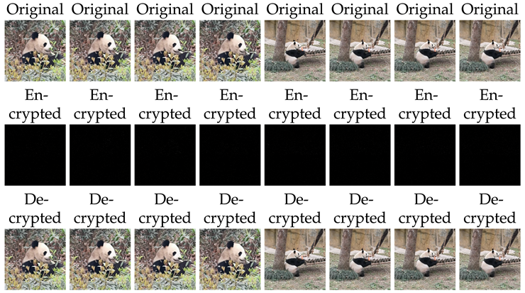

In the result, the average error between the numerical solution and the true solution is $2.7106\times {10}^{-9}$. The error of each frame is shown in the Table 1 as follows.

To further evaluate the quality of decrypted video, we use the Peak Signal-to-Noise Ratio (PSNR), Structural Similarity Index (SSIM) and Feature Similarity Index (FSIM) [33]. The results are summarized in Table 2. All PSNR values exceed 50, while both SSIM and FSIM values are 1, demonstrating the outstanding quality of our decrypted videos.

Example 3.

Let’s input two videos and finish local encryption and decryption using algorithms 5 and 6 by MATLAB: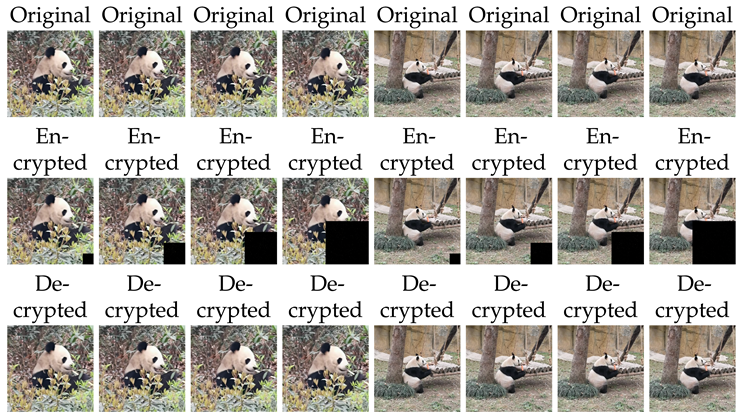

In the result, the average error between the numerical solution and the true solution is $8.9857\times {10}^{-10}$. The error of each frame is listed in the Table 3 as follows.

The results of PSNR, SSIM and FSIM are shown in Table 4. PSNR values all exceed 50, while both SSIM and FSIM values reach 1, indicating that the quality of local decryption is excellent.

6. Conclusion

The system of quaternion tensor equations (1) is universal, encompassing many other systems. This kind of system of quaternion tensor equations has practical applications in many areas. In this paper, we first transformed the quaternion tensor equations into quaternion matrix equations through the function f. By using the complex representation of split quaternion matrices and Moore–Penrose inverse, we presented a specific necessary and sufficient condition for the existence of a general solution to the system (1). When the solvability condition holds, we also derived the expression of the general solution to system (1). In particular, the unique solution was also given when the uniqueness condition held. Then we converted the obtained quaternion matrix solution back into a quaternion tensor solution using the function $f^{-1}$. Additionally, we established two algorithms to solve the system (1) and one example was given to prove the correctness of our results. In the last part, we provided the algorithms and two examples for color videos encryption and decryption using the system (1). In the future, we will focus on other systems of quaternion tensor equations over the split quaternion algebra.

References

- Hamilton WR, Lectures on quaternions, Dublin, Hodges and Smith, 1853.
- Took CC and Mandic DP, Augmented second-order statistics of quaternion random signals, Signal Processing, 91(2): 214-224, 2011.
- Miao J and Kou KI, Color image recovery using low-rank quaternion matrix completion algorithm, IEEE Transactions on Image Processing, 31: 190-201, 2021.
- Chen JF, Wang QW, Song GJ and Li T, Quaternion matrix factorization for low-rank quaternion matrix completion, Mathematics, 11(9): 2144, 2023.
- Jia ZG, Ling ST and Zhao MX, Color two-dimensional principal component analysis for face recognition based on quaternion model, Liverpool, Intelligent Computing Theories and Application: 13th International Conference, Part I(13): 177-189, 2017.
- Cockle J, LII. On systems of algebra involving more than one imaginary; and on equations of the fifth degree., London, Edinburgh, and Dublin, Philosophical Magazine and Journal of Science 35(238): 434-437, 1849.
- Adler SL, Quaternionic Quantum Mechanics and Quantum Fields., Oxford University Press, USA, 1995.
- Shoemake K, Animating rotation with quaternion curves., ACM SIGGRAPH Computer Graphics, 19(3): 245-254, 1985.
- Antonelli G and Chiaverini S, Kinematic control of a platoon of autonomous vehicles with a virtual leader., IEEE Transactions on Intelligent Transportation Systems, 8(4): 666-671, 2007.
- Krizhevsky A, Sutskever I and Hinton GE, ImageNet Classification with Deep Convolutional Neural Networks., Communications of the ACM, 60(6): 84-90, 2017.
- Carroll SM, Spacetime and Geometry: An Introduction to General Relativity (2nd ed.)., Cambridge University Press, 2019.
- Griffiths DJ and Heald MA, Introduction to Electrodynamics (4th ed.)., Cambridge University Press, 2013.
- Abadi M, Barham P, Chen J, Chen Z, Davis A, Dean J and Zheng X, TensorFlow: A System for Large-Scale Machine Learning., 12th USENIX symposium on operating systems design and implementation, (OSDI 16): 265-283, 2016.
- Paszke A, Gross S, Massa F, Lerer A, Bradbury J, Chanan G and Chintala S, PyTorch: An Imperative Style, High-Performance Deep Learning Library., Advances in neural information processing systems, 2019.
- Zhang S, Yao L, Sun A and Tay Y, Deep Learning Based Recommender System: A Survey and New Perspectives., ACM Computing Surveys, 52(1): 1-38, 2019.
- Qi LQ and Luo ZY, Tensor analysis: spectral theory and special tensors., Society for Industrial and Applied Mathematics, 2017.
- Qi LQ, Tensor Eigenvalues and Their Applications., Springer Nature, 2018.
- Ding WY, Luo ZY and Qi LQ, P-Tensors, P0-Tensors, and Their Applications., Linear Algebra and Its Applications, 555: 336, 2018.
- Wang QW, Lv RY and Zhang Y, The least-squares solution with the least norm to a system of tensor equations over the quaternion algebra., Linear and Multilinear Algebra, 70(10): 1942-1962, 2022.
- Xie MY, Wang QW and Zhang Y, The minimum-norm least squares solutions to quaternion tensor systems., Symmetry 14(7): 1460, 2022.
- Qin J and Wang QW, Solving a system of two-sided Sylvester-like quaternion tensor equations., Computational and Applied Mathematics, 42(5): 232, 2023.
- Chen XY and Wang QW, The η-(anti-) Hermitian solution to a constrained Sylvester-type generalized commutative quaternion matrix equation., Banach Journal of Mathematical Analysis, 17(3): 40, 2023.
- Ren BY, Wang QW and Chen XY, The η-Anti-Hermitian solution to a system of constrained matrix equations over the generalized segre quaternion algebra., Symmetry, 15(3): 592, 2023.
- Wang QW, Gao ZH and Xie LM, The (anti-)η-Hermitian solution to a novel system of matrix equations over the split quaternion algebra., Mathematical Methods in the Applied Sciences, 2024.
- Xie MY, Wang QW and Zhang Y, The BiCG algorithm for solving the minimal frobenius norm solution of generalized Sylvester tensor equation over the quaternions., Symmetry, 16(9): 1167, 2024.
- Yang LQ, Wang QW and Kou Z, A System of Tensor Equations over the Dual Split Quaternion Algebra with an Application., Mathematics, 12(22): 3571, 2024.
- Sun LZ, Zheng BD, Bu CJ and Wei YM, Moore–Penrose inverse of tensors via Einstein product., Linear and Multilinear Algebra, 64(4): 686-698, 2016.
- Liu TT and Yu SW, Some Properties of Reduced Biquaternion Tensors, Symmetry, 16(10): 1260, 2024.
- Yuan SF, Wang QW, Yu YB and Tian Y, On Hermitian solutions of the split quaternion matrix equation AXB+ CXD= E AXB+ CXD= E[J]., Advances in Applied Clifford Algebras, 27: 3235-3252, 2017.
- Ben-Israel A and Greville TNE, Generalized inverses: theory and applications., Springer Science & Business Media, 2006.
- Magnus JR, L-structured matrices and linear matrix equations., Linear and Multilinear Algebra, 14(1): 67-88, 1983.
- Xie LM and Wang QW, A system of matrix equations over the commutative quaternion ring., Filomat, 37(1): 97-106, 2023.
- Sara U, Akter M and Uddin MS, Image quality assessment through FSIM, SSIM, MSE and PSNR—a comparative study., Journal of Computer and Communications, 7(3): 8-18, 2019.