Submitted:
13 January 2025
Posted:
13 January 2025
You are already at the latest version
Abstract
The increasing reliance on water resources has necessitated improvements in turfgrass irrigation efficiency. This study aimed to compare measured field data with predicted data on irrigation water distribution in turfgrass rootzones to verify and enhance the accuracy of the HYDRUS-2D simulation model. Data were collected under controlled greenhouse conditions across unvegetated plots with two- and three-layered rootzone construction methods, each receiving 10 L m−2 h−1 of water for 1 h via subsurface drip irrigation (SDI) or sprinkler (SPR). Water content was monitored at various depths and time intervals. The hydraulic soil parameters required for the simulation model were determined through laboratory analysis. To improve model performance, sensitivity analysis, and model calibrations were conducted. The results indicated pronounced effects of the rootzone construction method and associated irrigation system on model quality performance. The calibrated models demonstrated good agreement with measured data, achieving model efficiency values (NSEs) up to 0.81 for SDI variants and 0.75 for sprinkler-irrigated variants. The findings suggest that HYDRUS-2D has potential as a cost-effective and efficient tool for evaluating irrigation strategies in turfgrass areas, although further refinement may be necessary for specific rootzone/irrigation combinations. This modeling approach can contribute to the optimization of irrigation scheduling and water use efficiency in turfgrass management.
Keywords:
turfgrass management
; turfgrass irrigation
; water use efficiency
; predictive models for irrigation
1. Introduction
Turfgrass areas provide a multitude of ecosystem services, social benefits, and economic advantages, particularly in urban areas [1,2]. These include carbon sequestration, which is crucial in mitigating climate change. Studies have shown that turfgrass systems can sequester significant amounts of carbon with specific management practices that enhance this capability [3,4,5]. For instance, managing irrigation and fertilization regimes can influence carbon sequestration rates in turfgrass, highlighting the importance of sustainable practices to maximize these benefits [4,5]. In addition to carbon sequestration, turfgrass contributes to various ecosystem services such as heat dissipation and water infiltration [6,7,8]. These services are particularly vital in urban settings, where green spaces help mitigate the urban heat island effect and improve overall environmental quality. The presence of turfgrass in urban landscapes enhances aesthetic value and supports recreational activities, thereby promoting social well-being [9,10].
Nevertheless, turfgrass requires the provision of conditions that support year-round sports activities, promote plant growth, and maintain a visually appealing appearance. Also, a good quality turfgrass cover needs more water compared to most other uses, necessitating a management system that minimizes water consumption.
The task at hand is to optimize the functionality of these systems while simultaneously guaranteeing their sustainability, a challenge that can be difficult to attain since improving one aspect might negatively impact the other [11]. As urban areas and their managed turfgrass spaces continue to expand, the environmental concerns surrounding them are expected to intensify. Emphasis on sustainability and ecological maintenance management has become increasingly important due to the growing pressure to address climatic change, particularly in preparing for impending water shortages [12,13,14,15]. It is crucial to integrate diverse aspects of playability, esthetic requirements, efficiency, and sustainability into a comprehensive and compatible compromise [16,17]. The need for irrigation in regions with insufficient rainfall to maintain healthy and aesthetically pleasing turfgrass has been a topic of significant discussion [18]. The efficiency of turfgrass irrigation is influenced by various climatic, technical, vegetation-related, and soil-physical factors. The rootzone construction method and irrigation system used are vital for achieving sustainable turfgrass areas [19,20].
To improve the efficiency of turfgrass irrigation, it is crucial to comprehensively assess the key factors and optimize the utilization of water in turfgrass areas to maximize irrigation efficiency. An investigation into the distribution of irrigation water under various construction methods and associated irrigation systems (sprinkler or subsurface drip irrigation) is crucial for predicting the success of the system’s design. This is because it significantly affects both irrigation scheduling and water efficiency [21,22].
The selection of appropriate rootzone construction methods with the central function of water retention (making it available to plants) and water transport (draining off excess water to maintain durability and playability) is a key factor for ensuring efficient water usage and the long-term sustainability of turfgrass areas. Sand-dominated rootzones are widely used for high-quality sports facilities because of their good drainage properties, greater air-filled pore space after compaction, and more consistent playing characteristics [23]. To increase the water-holding capacity, rootzones are amended with peat, and soil surfactants enhance moisture retention in turfgrass rootzones [24]. Common rootzone construction methods for turfgrass areas are multilayered systems, and many elementary and complex soil physical relationships can be identified in the soil matrix. Water retention and movement issues primarily influence decisions regarding sports turf construction methods [25]. Irrigation systems with high distribution accuracy and efficient water application can provide the basis for vital turf growth and sustainable use of water resources [26]. An efficient irrigation system should minimize the losses from wind drift, surface runoff, percolation, and evaporation [27]. Sprinkler irrigation systems are standard for turfgrass irrigation. These systems, using rotary, multi-jet, and spray sprinklers, are the standard for turf sports fields. Still, climatic factors such as wind drift and technically induced distribution inaccuracies may cause low irrigation efficiency, intensive percolation, and nutrient leaching in the soil matrix, which is weak in sorption and water retention [28,29].
In contrast, subsurface drip irrigation (SDI) systems are characterized by direct water delivery into the plant root zone, which can increase the irrigation system´s efficiency [30]. Subsurface drip irrigation systems typically use either point or linear sources for water supply. Linear-source systems (“porous pipes”) feature uniform water flow along the entire length of the line, whereas point-source systems, commonly referred to as drip lines, are equipped with non-pressure-compensating or pressure-compensating drippers. These SDI systems employ polyethylene pipes placed at various depths and distances and are customized to the specific plants being irrigated [31].
The rootzone construction method, along with the choice of irrigation system (sprinkler, SDI, or hybrid approach), constitutes a highly intricate design in terms of irrigation water distribution [32]. However, numerical simulation models such as HYDRUS-2D can be used to predict soil water distribution for different construction methods, irrigation systems, and irrigation strategies quickly and efficiently [33,34] and have proven to be particularly reliable and versatile [35]. Both in research into subsurface irrigation in agriculture [36,37,38] and in other ecosystems (e.g., urban greens) [39], reliable agreement between HYDRUS simulations and the actual water distribution in field trials in various soils has been demonstrated [37,40,41]. The basis of modeling water behavior in unsaturated porous media lies in describing the media’s pore structure, as evidenced by the water retention curve and the unsaturated hydraulic conductivity function. These functions are indispensable for simulating variations in water content and flux [42].
A well-known parametric model that connects volumetric water content to matric potential was introduced by van Genuchten [43], which incorporates parameters such as ϴr, ϴs, α, n, and m. This model has been extensively used in various studies [44,45] and is integrated into the HYDRUS-2D model as follows:
where is the water content at matric potential ; ϴr is the residual water content (cm3 cm−3); ϴs is the saturated soil water content (cm3 cm−3); α, n, and m describe the shape of the function without physical meaning; and m is usually fixed as 1 − 1/n [36].
The previously discussed formulation can be integrated with Mualem’s equation [46] to elucidate the unsaturated hydraulic conductivity function, and it is also incorporated in the HYDRUS-2D model:
with
where is the hydraulic conductivity at matric potential ; Ks is the saturated hydraulic conductivity; Se is the effective water content; L is a parameter describing the pore structure of the soil, usually set to 0.5; and m is fixed as m = 1 − 1/n [33,47,48].
Rootzone materials, characterized by a high content of coarse pores, often exhibit poor re-wettability after drying due to air entrapment or issues with the wetting of organic materials. This phenomenon, known as hysteresis of the water retention curve [47,49], has been demonstrated to be particularly significant under SDI in several studies [36,48,50]. Consequently, when rewetting occurs at a specific matric potential, the material's water content will not achieve the same level as measured during the drying process. Thus, it is imperative to incorporate the effects of hysteresis into the retention function of the HYDRUS model to attain more precise model results, which requires that both the main drying and main wetting curves are known [51,52,53].
The HYDRUS code incorporates the description of the main drying curve through the soil hydraulic parameters ϴr, α, n, and ϴs. Differences between measured and calibrated values are often due to not considering hysteresis in the wetting curve [45]. Based on the study of Kool and Parker [54] for hysteretic description in the wetting curve, the soil hydraulic parameter αw was employed. Their research indicated that α was the sole parameter to change for considering hysteresis, and they determined that the range of αw/α is sufficiently narrow that assuming αw/α ≈ 2 should provide a useful approximation in cases where data are lacking (where the subscript w indicates wetting). Additionally, the soil hydraulic parameter ϴsw was implemented based on the study of Simunek et al. [33], who posited that αw and ϴsw are the only independent parameters necessary to describe hysteresis in the retention curve. Huang et al. [55] used hydraulic parameters αw and nw as variables to describe hysteresis and found in their comparison with the Kool and Parker model that their formulation yielded higher accuracy.
Physically based models, such as HYDRUS-2D, often require only minimal calibration when all the required input parameters (e.g., hydraulic parameters for water flow in soil) have already been independently determined [56]. Calibrating a model involves adjusting the input parameters of the odel to fall within reasonable ranges until the simulated results closely match the measured data [57]. In cases where hysteresis is a relevant factor, the parameters describing hysteresis may also need calibration.
Understanding the sensitivity of the soil hydraulic parameters helps to decide which parameters may be used for calibration (i.e. the most sensitive ones). In a study [58,59], which tested the sensitivity of soil hydraulic parameters in the HYDRUS-2D model, it was revealed that parameter n was the most sensitive parameter for the simulation output (soil water content), followed by the saturated soil water content ϴs while Ks was the least sensitive parameter.
According to Ghazouani et al. [60], HYDRUS tended to overestimate the modeled water contents when compared to the measured ones, which could be attributed to an imperfect parameterization of the soil hydraulic functions. Nevertheless, when accurately described and parameterized, HYDRUS demonstrated its ability to provide reliable values [61].
Widely used measures for evaluating the model quality are based on statistical indicators, namely the root mean square error (RMSE), mean absolute error (MAE), correlation coefficient (R2), and Nash-Sutcliffe efficiency (NSE), which indicate acceptable quality at values > 0.5 [36,61].
Although HYDRUS-2D is a widely used numerical model for predicting water, heat, and solute movement and distribution, no work has been carried out to verify the accuracy of this model for simulating irrigation water distribution under sprinkler and SDI systems across various multilayered rootzone construction methods for turfgrass areas.
This study aimed to compare experimentally measured greenhouse data with predicted data on irrigation water distribution. The objectives were i) to verify and enhance the accuracy of the HYDRUS-2D model, ultimately providing an affordable and rapid tool for evaluating efficient irrigation scheduling in turfgrass areas, ii) to determine the sensitivity and the necessity of a precise parameterization of the soil hydraulic parameters to achieve a high model accuracy, iii) to use the calibrated model to determine if dividing the total irrigation quantity into multiple smaller applications will enhance irrigation efficiency, and iv) to decide based on the calibrated model if a hybrid-irrigation approach (sprinkler-irrigation plus SDI) inhances irrigation efficiency compared to sprinkler or SDI alone.
2. Materials and Methods
This study used three different rootzone construction methods (2A, 2B, and 3) and two different irrigation systems (sprinkler and subsurface drip irrigation) to verify and enhance the model quality and evaluate efficient irrigation scheduling in turfgrass areas.
2.1. Experimental Setup and Measurements
Experimentally measured data were collected under greenhouse conditions using bare soil profiles (plots with no grass cover).
The research area (11.94 m × 4.71 m including non-considered edge areas of the actual test plots) was designed as a completely randomized two-factorial split plot with three replications for each treatment. The total area comprised six main plots (each 4.11 m × 1.70 m; three for SPR and three for SDI irrigation). Each of the six main plots was divided into three plots (1.70 m × 1.37 m) for the three construction types (two 2-layered and one 3-layered design). Two different irrigation cycles with discharge amounts of cycle 1 = 10 mm (the usual irrigation amount for turfgrass) and 2 = 20 mm (data cycle 2 not shown) were applied, both with an intensity of 10 mm h−1. After irrigation cycle 1, all plots underwent a drying phase (approximately four weeks with an average evaporation rate of 3.22 mm day−1) to achieve a uniform initial soil volumetric water content. The initial volumetric water content was between 9 and 10 vol.% without significant differences between the plots.
A total of five materials—STD, UHFC (rootzone layer), URTS F (intermediate layer), URTS C, and DS (gravel drainage layers)—were used for the three construction types. Table 1 lists the physical properties of each material.
STD is generally used for sports turf areas with a common requirement for functionality and sorption capability, consisting of sand, peat, and humus-rich topsoil. The UHFC (ultra-high-function) material, also consisting of sand and peat but without topsoil, has high functionality at the expense of sorption capability with a lower silt content than STD. It also exhibits higher hydraulic conductivity while maintaining a water-holding capacity (field capacity) similar to that of STD.
URTS F is an intermediate layer material consisting of medium-sized sand (grain size up to 0.5 mm) with very low silt content, with a much higher hydraulic conductivity and lower water-holding capacity (field capacity) than STD and UHFC.
DS is a gravel drainage layer material with a 0–8 mm particle size distribution, higher hydraulic conductivity, and lower silt content than the rootzone materials (STD and UHFC). URTS C is a much finer drainage material consisting of very coarse sand with a grain size of up to 2 mm, much higher hydraulic conductivity, and lower bulk density than DS. The construction layers had a total thickness of 24 cm, consisting of rootzone layers (0–12 cm), plus gravel drainage layer (12–24 cm) for the 2-layered constructions, or plus intermediate layer (12–18 cm) and drainage layer (18–24 cm) for the 3-layered constructions, and with an underlying 26 cm sand carpet base with a grain size up to 2 mm for surface drainage (Figure 1). Three rootzone construction methods were applied. Two construction types (2A and 2B) according to the German Standards for Sports Grounds [66] consisted of a 2-layered design, including a 12 cm peat-amended sandy rootzone (STD or UHFC) over a 12 cm gravel drainage layer (DS) with a total thickness of 24 cm. One construction method (3) comprised a 3-layer design based on the guidelines of the United States Golf Association (USGA, 2018) that included a 12 cm rootzone (UHFC) over a 6 cm intermediate sand layer (URTS F) and an underlying 6 cm drainage layer (URTS C).
Figure 1 provides an overview of the construction types, associated materials, and irrigation systems.
In each case, all materials were installed with a bulk density of 95% of the standard Proctor density [66] (STD = 1.55, UHFC = 1.46, URTS C = 1.60, URTS F = 1.41, DS = 1.80 g cm−3) and two systems used for irrigation. Due to the plot size and to maximize the water distribution uniformity, sprinkler-irrigated plots were hand-watered with a discharge rate of 10 mm h−1. The subsurface drip irrigation system (SDI) used was a line-source drip system consisting of porous pipes (radius r = 0.9 cm) with a discharge rate of 3 L h−1 m−1 and 9.09 L h−1 m−2, respectively, resulting from a line spacing of 33 cm. The SDI installation depth was 16.5 cm, and the operating pressure was 0.2 bar.
The collected dataset for each evaluated sprinkler or SDI irrigated variant (2A, 2B, and 3) comprised 30 measurements (n=30), which were derived from a) three distinct observation depths (3, 6, and 12 cm) and b) ten specific observation times (0.00, 0.17, 0.33, 0.50, 2.00, 4.00, 8.00, 12.00, 24.00, 48.00 hours after irrigation initiation). Data were collected in two separate operations during both cycles and to ensure an identical initial volumetric water content (VWC), irrigation cycle 2 commenced following a drying phase of three weeks. Soil samples were taken with a soil sampler through lateral openings at −3, −6, and −12 cm using a 50 mm diameter metal tube, which was driven into the soil and withdrawn. The soil gravimetric water content was measured by oven-drying the soil samples at 105 °C, and the VWC was calculated by multiplying it with bulk density. For each replication and observation time, a total of 15 soil samples were collected from five measurement points (center of the plot above the SDI line and at 8.25 and 16.5 cm right and left of the center; at similar positions for the SPR variants) and at depths of 3, 6, and 12 cm. The five water content values for one depth for each sampling were averaged. After sampling, the voids were refilled with the same soil material.
2.2. Simulation Model, Initial and Boundary Conditions
HYDRUS-2D (H2D) finite element model version 5.04 [56] was used to simulate the distribution of irrigation water in bare soil profiles. The simulation was initiated by creating a model setup with the correct material layers, initial conditions, and boundary conditions within H2D that corresponded to the experimental setup.
The observed volumetric soil water content in the soil profile was taken as the initial water content for all simulated scenarios. The model´s soil surface was subjected to atmosphere boundary conditions for soil water evaporation (EV) corresponding to greenhouse conditions with 0.013 cm h−1. A free drainage boundary condition was imposed at the bottom of the soil profile. On the right- and left side of the soil profile, a no-flux boundary was used (Figure 2).
Sprinkler irrigation was scheduled in accordance with the experimental setup with an intensity of 1 cm h−1. For SDI, a variable flux boundary was used around the SDI emitter (Figure 2). During irrigation, the drip pipe boundary had a constant water flux, which was obtained by dividing the emitter discharge flow rate of 3 L (h × m)−1 by the surface of the drip pipe as:
During the no-irrigation period, the flux was kept at zero.
The simulation model domain was 50 cm deep. The high differencesbetween the soil hydraulic parameters of the different materials, as well as the significant temporal-spatial variability under SDI, necessitated a node spacing of 0.50 mm, with progressively closer spacing down to 0.25 mm around the SDI pipe and each layer interface.
2.3. Model Quality Evaluation Criteria
The evaluation of the HYDRUS-2D model encompassed the assessment of model quality, sensitivity analysis, and model calibration based on the predicted and measured volumetric soil water content dataset (n=30) of each variant within the upper 12 cm. This specific depth was chosen as it typically represents the rooting zone of cool-season turfgrass [67].
The correlation coefficient (R2), root mean square error (RMSE), mean absolute error (MAE), and Nash-Sutcliffe efficiency (NSE) were calculated using the following equation to assess the model quality parameters:
where Xi = the measured volumetric water content (cm3 cm−3), Yi = the predicted volumetric water content (cm3 cm−3), Xav = the average of the measured volumetric water content (cm3 cm−3), and N = the number of observations.
The correlation coefficient should be close to 1. The root mean square error (RMSE) is a commonly utilized metric for evaluating the agreement between measured and simulated values and should be close to zero. A widely accepted standard that does not consider over- or under-forecasting is the mean absolute error (MAE). In an ideal scenario, the MAE should be nearly zero. Both the root mean square error (RMSE) and mean absolute error (MAE) share the same units as the measured and predicted values [68]. Lastly, the Nash-Sutcliffe efficiency NSE [69] is a normalized statistic commonly used to evaluate hydraulic models and compares residual and measured variance [70]. The parameter equals zero when the square of the differences between the measured and predicted values equals the variability in the measured data. If the NSE value is negative, the measured mean is a more accurate predictor than the model [71]. If the model gives perfect results, the NSE = 1. An acceptable-quality model should have an NSE > 0.5 [68].
2.4. Input Parameter, Parameter Sensitivity and Model Calibration
The water retention drying curves were determined using Eijkelkamp standard sandbox apparatus [72] to assess the water content at pF 1, 1.8, and 2.5. The water content at pF 4.2 was determined using a pressure plate apparatus, as per the DIN EN ISO 11274 (2019) [65]. The soil water retention curves were then parameterized according to the van-Genuchten equation [43] by adjusting the θr (residual water content), α, and n (shape factors) values using the EXCEL solver function to match the measured water content and water suction drying curve values. The saturation water content θs was fixed at the total porosity (TP). The material´s hysteretic behavior was evaluated based on the capillary rise of water in the materials employed in this study within experimental containers composed of 10 rigid plastic rings, each measuring 2 cm in height [36]. The rings were filled with the material of interest (95% bulk density of Proctor density DPR), and a flooding depth of 1 cm was maintained for 48 h before the water content was determined gravimetrically. It was assumed that the water tension in the rings is defined by the distance to the water table, and the water content at equilibrium is analogous to the water retention curve [47]. The wetting water retention curve was initially parameterized by adjusting and establishing the parameter α to αw [33]. The parameters used in HYDRUS-2D are presented in Table 2.
Sensitivity analyses and model calibration focused on the materials used in the top two layers, including STD, UHFC (rootzone layers), URTS F (intermediate layer), and DS (gravel drainage layer) within each construction method (2A, 2B, and 3) and irrigation system (SDI and SPR). The HYDRUS-2D model was used to analyze the sensitivity of the soil hydraulic parameters θr, α, and n (representing the soil water retention drying curve parameterization) while excluding the exact analytically determinable parameter θs (fixed at total porosity), as well as the parameters αw and θsw (representing the opportunities in the HYDRUS code for describing material´s hysteresis behavior). The study evaluated the impact of a 20% incremental increase in these parameters on simulation output (VWC) after 10 mm irrigation (cycle 1) regarding the deviation in model efficiency (NSE).
The HYDRUS-2D software package’s inverse solution function was employed for model calibration. This process utilized the four parameters identified as most sensitive through sensitivity analysis (scenario F1–F4). Additionally, based on previous research [33,45,54,55], a combined calibration approach was applied to the parameters αw and n, as well as αw and ϴsw (scenario F5–F6). Six different scenarios (F1–F6) were used for the calibration procedures. The HYDRUS inverse solution was used to independently calculate the calibrated values of the materials used in the top two layers (STD, UHFC, URTS F, DS) for each combination of construction method (2A, 2B, 3) and irrigation system (SPR, SDI).
2.5. Irrigation Scheduling Development
The HYDRUS-2D code was also used in hypothetical instances to examine the effect of irrigation treatments, which are given in Table 3. The parameters for the boundary and flow domain remained unchanged from previous descriptions. Based on previous research [73] that demonstrated the favorable water retention characteristics of the three-layered construction method 3, this methodology was employed to evaluate the efficacy of various irrigation approaches regarding water usage.
The analysis focused on two key factors influencing irrigation efficiency, i.e. drainage flux and soil water storage within the simulation domain (upper 50 cm). Four different irrigation approaches were assessed. Each approach involved applying a total irrigation amount of 10 mm through either sprinkler (SPR 1–4), SDI (SDI 1–4), or HYBRID (HYBRID 1–4) in up to five irrigation events within a 12 h period.
3. Results
3.1. Model Quality Evaluation
The model's performance was evaluated using the model efficiency parameter NSE, and the results were graphically visualized by comparing the observed values against the simulation output differences, presented through spatial maps (ordinary Kriging method).
Figure 3 shows the observed values (left) against the difference values (right) of construction methods 2A, 2B, and 3 under sprinkler irrigation, each averaged across the entire observation time 0-48 hours following 10 mm irrigation. Figure 4 is analogous to Figure 3, but in each case under SDI.
The model’s effectiveness, measured by Nash- Sutcliffe efficiency (NSE), ranged from 0.58 (2B) to 0.68 (2A) and 0.72 (3) for sprinkler-irrigated variants (generally achieving NSE values above 0.5) and from 0.27 (2A) to 0.48 (3) and 0.52 (2B) for SDI variants. The highest model performance was observed in the 3_SPR variant (NSE = 0.72), whereas the poorest performance was observed in the 2A_SDI variant (NSE = 0.27).
Additionally, graphical analysis showed that, for sprinkler-irrigated variants 2A and 2B, the model tended to calculate higher predicted values than observed values. At an observation depth of 6 cm, the average overestimation was 0.85 vol. % for 2A and 1.22 vol. % for 2B. At a depth of 12 cm, the average overestimation was 0.94 vol. % for 2A and 1.55 vol. % for 2B. In the case of SDI, an average overestimation within variant 2A of 1.27 vol. % (6 cm depth) and 3.11 vol. % (12 cm depth) was observed. In contrast, variant 3_SDI exhibited a different pattern, with the model generating lower predicted values than the observed ones. The average underestimation was 1.54 vol. % at a depth of 6 cm and 2.27 vol. % at a depth of 12 cm. Similar to the model’s performance, variant 3 showed the most minor differences among sprinkler-irrigated variants, while 2B displayed the least variation among SDI variants.
3.2. Sensitivity Analysis
The sensitivity analyses of the 5 parameters ϴr, α, n (normal drying WRC), ϴsw , and αw (wetting WRC) presented in Figure 5 illustrate the respective deviations in model efficiency (NSE) under a soil hydraulic parameter perturbation of +20% within each variant's upper two layers (Layer 1 and Layer 2). The results demonstrated that the parameter perturbation elicited contrasting sensitivity responses across the evaluated variants.
Generally, it could be observed that the materials within Layer 1 reacted more sensitively under a soil hydraulic parameter alteration compared to Layer 2 with an average NSE increase (absolute value across all parameters and variants) of 0.14 compared to 0.05, respectively (Table S1 in the supplement).
Further, among the five parameters examined, α consistently exhibited the least sensitivity with a maximum NSE deviation of −0.04 (3_SDI, Layer 1) and 0.04 (2A_SDI, Layer 2), while parameter n demonstrated the highest sensitivity with a maximum NSE deviation of −0.62 (3_SPR, Layer 1). An analysis of parameter n variations revealed that four out of six variants in both layers showed negative NSE deviations. The exceptions were variants 2A_SPR and 2A_SDI in Layer 1 and 2B_SDI and 3_SDI in Layer 2.
Parameter ϴsw had the second highest sensitivity, and the NSE deviation ranged from 0.14 (3_SDI) to −0.33 (2A_SDI) in Layer 1 and from 0.09 (2A_SDI) to −0.11 (2B_SDI) in Layer 2.
Summarizing, based on the absolute averaged NSE deviation (across all parameters and variants), the four most sensitive parameters are as follows (Table S1 in the supplement):
n (0.35) > ϴsw (0.14) > ϴr (0.11) > αw (0.04) within Layer 1;
n (0.11) > ϴsw (0.05) > αw (0.04) > ϴr (0.02) within Layer 2.
3.3. Model Calibration
The results of model calibration calculated using the HYDRUS-2D inverse solution are presented for each material (STD, UHFC, DS, and URTSF) and scenario (F1–F6) in Table 4. The influence of model calibration scenarios F1–F6 on model efficiency (NSE) is illustrated in Figure 6.
Notably, substantial variations are observed depending on whether the calibration is incorporated into Layer 1 (L1) or Layer 2 (L2) or if it is implemented across both upper layers, Layer 1 and 2 (L1+L2). In general, the sprinkler-irrigated variants, which exhibited already Nash-Sutcliffe efficiency (NSE) values exceeding 0.50 under laboratory-measured default settings, demonstrated only a minor improvement across all model calibration scenarios (between +0.07 and +0.01).
Within the SDI variants, generally, model calibration scenario F5 pushed the NSE values to a range of > 0.50, whereby the greatest improvement could be achieved with the combined implementation of both layers (L1+L2), and the values increased in 2A_SDI from 0.27 to 0.79, in 2B_SDI from 0.52 to 0.81, and in 3_SDI from 0.48 to 0.76
The impact of the model calibration scenarios on the average model efficiency values across the SDI variants was ranked in descending order as follows (details in Table S2 in the supplement):
F5_L1+L2 (0.79) > F5_L1 (0.68) > F5_L2 = F4_L1 (0.63).
This indicates, that scenario F5 (i.e. calibration αw and n) resulted in the highest gain in efficiency and should be used for further simulations.
Figure 7 illustrates the regression analysis of the measured values (n=30) in comparison with the simulated volumetric water content under the default settings (without calibration) and across the highest NSE improvement scenario F5 (sprinkler F5_L1 and SDI F5_L1+L2), including the correlation coefficient (R2), slope of the regression lines (SLOPE), root mean square error (RMSE), and mean absolute error (MAE).
Correlation coefficient (R2), RMSE, and MAE values across the sprinkler-irrigated variants were between 0.72 and 0.79, 1.45 and 1.75 vol. %, and 1.09 and 1.46 vol. %, respectively, under default settings and developed to 0.73–0.83, 1.42–1.49 vol. %, and 1.02–1.15 vol. %, respectively, under model calibration scenario F5_L1.
Within the SDI variants, the values were between 0.44 and 0.81, 1.58 and 3.03 vol. %, and 1.20 and 2.28 vol. %, respectively, under default settings and developed to 0.75–0.84, 1.11–2.18 vol. %, and 0.77–1.71 vol. %, respectively, under model calibration scenario F5_L1+L2.
Generally, the correlation coefficients (R2) were greater across the calibrated SDI variants (0.75–0.84) than across the calibrated sprinkler-irrigated variants (0.73–0.83). Nevertheless, the slopes of the regression lines were closer to 1 within the sprinkler-irrigated variants compared to SDI variants and ranged from 0.81 (3_SPR) to 1.04 (2B_SPR) and 0.65 (3_SDI) to 0.95 (2A_SDI), respectively.
3.4. Irrigation Scheduling Evaluation
The results of the HYDRUS-2D code of the three-layered construction method 3, which were utilized in hypothetical instances to examine four different irrigation approaches (IA1: 10 mm irrigation at time zero; IA2: 75% at time 0 and 25% after 6 hours; IA3: 50% at time 0, and 25% each after 6 and 12 hours; IA4: 50% at time 0, and 12.5% after 3, 6, 12, and 18 hours; see Table 4). The results are shown in Figure 8 (and Table S3 in the supplement). These observations were made at various times (4–48 h) after 10 mm irrigation (sprinkler, SDI, or hybrid). Different behavior was observed across the irrigation approaches concerning the soil storage of irrigation water and drainage flux.
Up to 12 hours (8 hours for IA1), the water storage was very similar within the irrigation approaches with a tendency of generally minimal higher water storage in the SDI variants. Generally, the water storage was higher in IA1 and IA2 compared to IA3 and IA4. Strong differences could be identified between the water storage in the different irrigation systems after 24 hours: the SPR variant always showed the lowest water storage followed by the SDI irrigation. The hybrid irrigation system always had the highest water storage. The hybrid-approach results at 48 h were 3.33 mm (IA4), 3.61 mm (IA3), 2.69 mm (IA2), and 2.39 mm (IA1) (Figure 4). Since the cumulative drainage is naturally determined by the water storage, these values were always inversely related to the storage (Figure 4).
In summary, focusing on the maximum residual soil water storage and minimum drainage flux of each irrigation technique (SPR, SDI, HYBRID) and approach (IA1—IA4) at an observation time of 48 h, the following order was observed for soil water storage:
HYBRID-IA3 (3.61 mm) > SDI-IA4 (2.53 mm) > SPR-IA3 (0.38 mm),
and for drainage flux:
HYBRID-IA3 (2.57 mm) < SDI-IA4 (3.59 mm) < SPR-IA3 (5.46 mm).
The difference of water storage plus drainage flux to the 10 mm irrigation is due to the actual evaporation during the 24 hours.
4. Discussion
Turfgrass areas, regardless of whether they are golf courses or sports fields, offer numerous ecosystem services, including carbon sequestration, oxygen production, water and air purification, heat dissipation, and water infiltration, which are vital for mitigating climate change and improving urban environmental quality [1,2,74]. Additionally, they enhance aesthetic value and support recreational activities, contributing to social well-being in urban landscapes. [9,10].
Nevertheless, adequate drainage is essential for all turfgrass areas, as it facilitates the removal of substantial volumes of water and prevents the cancelation of events due to waterlogging and unstable playing surfaces. Conversely, the rootzone construction method and associated irrigation systems must support efficient irrigation water usage, uniform soil moisture distribution, and adequate soil moisture retention to maintain acceptable turfgrass quality and create a complex system regarding soil water dynamics.
For this purpose, HYDRUS-2D is an affordable and widely utilized numerical predictive model and a valuable tool for evaluating efficient irrigation scheduling. To analyze and enhance the accuracy of this model, we compared experimentally measured greenhouse data with the predicted data of the model concerning irrigation water distribution.
The results of this study demonstrated the efficacy of the HYDRUS-2D model in simulating irrigation water distribution, with the need for model calibration among multilayered rootzone construction methods, particularly in the context of subsurface drip irrigation.
4.1. Theoretical Aspects
The model performance varied depending on the construction method and the irrigation system used. Initial model simulations of water content utilizing default (laboratory-measured) parameters demonstrated acceptable to high performance for sprinkler irrigation (NSE 0.58–0.72) but suboptimal performance for SDI (NSE 0.27–0.52). The model tended to overestimate the two-layered sprinkler irrigation and SDI variants, consistent with Ghazouani et al. [60], who reported overestimation of modeled water content values compared to measured values, with 2A_SDI displaying the lowest model accuracy. In contrast, the three-layered SDI variant notably underestimated soil water content, particularly in the lower parts of the rootzone (observation depths of 6 and 12 cm).
Sensitivity analysis of the parameters indicated that the shape factor n exhibited the highest sensitivity within both layers and across all variants, whereas shape factor α (drying WC) demonstrated the lowest sensitivity, which is consistent with the results of Inoue et al. [58]. Soil hydraulic parameter ϴsw shows the second highest sensitivity, aligning with the findings of Abbasi et al. [59]. The sensitivity analysis further demonstrated the need for the precise parameterization of soil hydraulic parameters, as construction method 2B/Layer 2 exhibited a decrease in the Nash-Sutcliffe efficiency (NSE) value of −0.23 when the shape factor n was increased by 20% under sprinkler irrigation. In contrast, this modification increased the NSE value of +0.19 under subsurface drip irrigation (Figure 5).
The calibrated αw (wetting WRC) values resulted in αw/α ratios averaging 1.90 across all variants (calibration scenario 1), indicating substantially greater αw values than the corresponding drying curve values. This finding aligns with the study of McCoy and McCoy [45] and approximates the value of 2 (αw/α ratio) suggested by Kool and Parker [54] for estimating wetting curve parameter αw. This supports using this approximation when measured wetting curve data are unavailable. The shape factor n shows changeable behavior within calibration scenarios F2 and F5 with a partially low to strongly pronounced increase and decrease depending on the construction method and associated irrigation system; these findings do not agree with the results of McCoy and McCoy [45], which showed lower n values when considering the typical characteristics of the hysteresis wetting curve response. Nevertheless, our findings suggest that, particularly under subsurface drip irrigation conditions, the shape parameter nw(wetting curve) should be additionally considered within the HYDRUS code, along with αw, to describe the hysteresis behavior of the material more accurately.
Following calibration, the model strongly agreed with the measured data, achieving a Nash-Sutcliffe efficiency (NSE) value of up to 0.81 for subsurface drip irrigation (SDI) and 0.75 for sprinkler irrigation.
Calibration demonstrated that under sprinkler irrigation, the variants exhibited NSE values > 0.5 already under laboratory-measured default settings and revealed only slight improvement after calibration. Calibration is therefore not necessary, at least under the conditions investigated. If calibration is to be carried out anyway, consideration of layer 1 is sufficient.
In contrast, under SDI, a significant improvement in model quality could be observed by considering both layers (Layers 1 and 2). A plausible explanation is that during SDI, the model primarily utilized the wetting retention curve in Layer 2. However, during drainage and redistribution, both layers and their corresponding wetting and drying curves and the connections between them necessitated consideration within the model calibration procedure.
The soil hydraulic parameters for each material were independently calibrated using the HYDRUS inverse solution method. However, the results demonstrated that the model structure significantly influenced the calibrated material's soil hydraulic properties, as evidenced by the high variability in the calculated soil hydraulic parameters. For instance, across construction methods 2A_SPR and 2A_SDI, the shape factor αw exhibited values ranging from 0.152 to 0.388 (Table 4). Furthermore, the models revealed pronounced gradients at the interface between neighboring layers (Layers 1 and 2) due to markedly different soil physical properties of the materials employed. For instance, in construction method 3, Layer 1 (UHFC) demonstrated a saturated hydraulic conductivity (Ksat) of 649 mm h−1, while Layer 2 (URTSF) showed a value of 1465 mm h−1. Similarly, substantial water content and water suction gradients are observed at the interface of Layer 1 and 2 in construction method 2A, where Layer 1 exhibited a Ksat of 220 mm h−1 and Layer 2 had a Ksat of 916 mm h−1. These findings indicate that complex model structures involving multilayered rootzone construction methods comprising adjacent layers with significantly different soil physical properties necessitate model calibration, particularly under subsurface drip irrigation conditions.
Notwithstanding the observed local variations, the NSE values consistently remained positive, indicating substantial agreement between the measured soil water content and the model’s simulated values [69] despite the complexity of the conditions to which the model was subjected, that is, multi-layered rootzone construction methods and irrigation systems with high spatial variability.
4.2. Practical Significance
Despite discrepancies between the calculated and measured values of soil water content, these variations typically remained below 4 vol. % and are consistent with standard field measurement uncertainties. These uncertainties are significantly influenced by the specific measurement technology employed (e.g., measurement with a frequency domain reflectometry (FDR) sensor), the measurement point's location, and the measurement's timing. Regarding practical significance, it is essential to note that the model demonstrates efficacy in multilayer construction methods with highly complex soil physical relationships and under irrigation systems with considerable spatial variability (i.e., SDI), significantly influencing irrigation water dynamics [75]. Consequently, this tool facilitates the adaptation of irrigation management to the specific onsite structural conditions of sports turf areas and enables the implementation of efficient irrigation practices.
In the context of irrigation scheduling evaluation, the model data of the three-layered variant (construction method 3) indicated that, under sprinkler irrigation, dividing the total irrigation water quantity into multiple smaller applications (approaches 3 and 4) generally resulted in higher soil water storage and lower drainage flux compared to single large applications. Furthermore, the model data under the hybrid irrigation approach indicated the most efficient use of resource water, characterized by the highest soil water storage and lowest drainage flux compared to the other irrigation approaches (Figure 8). The practical applicability or the requirement profile of an irrigation technique should also be emphasized, as maintenance practices typically conducted on turfgrass areas necessitate surface irrigation (i.e., sprinkler) for establishing seeding or flushing in granulated fertilizers. In the context of turfgrass irrigation, the primary focus remains on the targeted application of irrigation water into the root zone, which should ideally be applied with minimized evaporation loss, surface runoff, and moisture penetration of the turf to reduce disease pressure. The results indicate that under a hybrid irrigation approach, these requirements are attainable, further demonstrating the potential of HYDRUS-2D as a cost-effective and valuable tool for evaluating and optimizing turfgrass irrigation strategies.
4.3. Limitations of the Study and Further Research
While the calibrated models exhibited strong overall performance, some discrepancies between measured and predicted values remained, particularly for the three-layered construction under SDI. This suggests that further refinement of the HYDRUS code, such as implementing nw as an additional shape factor, may be necessary to account for the material's hysteresis behavior more precisely. Moreover, to evaluate the fundamental model performance across various rootzone construction methods and irrigation systems, the study was conducted on bare soil profiles, and the incorporation of turfgrass and its associated root water uptake patterns would undoubtedly influence water distribution and irrigation efficiency.
Future research should incorporate root water uptake models to provide a more comprehensive understanding of soil-plant-water dynamics and relationships in multi-layered construction methods for turfgrass areas, wherein an increasing complexity for model calibration could be anticipated.
5. Conclusions
This study demonstrated the efficacy of the HYDRUS-2D model in simulating irrigation water distribution across various turfgrass rootzone construction methods. The key findings include the following: (i) The initial model performance varied depending on the construction method and irrigation system, with acceptable to high performance for sprinkler irrigation (NSE 0.58–0.72) but suboptimal performance for subsurface drip irrigation (SDI) (NSE 0.27–0.52). (ii) Sensitivity analysis revealed that the shape factor n exhibited the highest sensitivity, whereas the shape factor α showed the lowest sensitivity across all variants. Model calibration significantly improved the performance, achieving Nash-Sutcliffe efficiency (NSE) values up to 0.81 for SDI and 0.75 for sprinkler irrigation, respectively. This calibration appears necessary to enhance model quality among multilayered rootzone construction methods, particularly in the context of subsurface drip irrigation. The calibrated αw/α ratios averaged 1.90 across all variants, aligning with previous research and supporting this approximation when the measured wetting curve data are unavailable. (iii) The evaluation of irrigation scheduling approaches revealed that dividing the total irrigation water quantity into multiple smaller applications generally resulted in higher soil water storage and lower drainage flux than single large applications. (iv) A hybrid irrigation approach combining sprinklers and SDI systems showed the most efficient use of water resources.
While the calibrated models demonstrated good overall performance, some discrepancies between the measured and predicted values persisted, particularly for the three-layered construction under the SDI. This finding suggests that further refinement of the model is necessary. These findings indicate that HYDRUS-2D has the potential to be an efficient tool for evaluating irrigation strategies in turfgrass areas. However, future research should incorporate root water uptake models to provide a more comprehensive understanding of soil-plant-water dynamics in multilayered construction methods for turfgrass areas.
Overall, this modeling approach has the potential to optimize irrigation scheduling, thereby enhancing water-use efficiency in turfgrass management. Consequently, this optimization improves the sustainability, capacity for carbon sequestration, and ecosystem services of turfgrass, which are particularly crucial in urban settings.
Supplementary Materials
The following supporting information can be downloaded at the website of this paper posted on Preprints.org. Table S1. Influence of 20% perturbation of soil hydraulic parameters θr, n, θsw, αw, and Ksw on the absolute model efficiency deviation (ABS NSE deviation) across Layer 1 and Layer 2 of the variants 2A_SPR–3_SDI, irrigation cycle 1 (10 mm). Table S2. Model efficiency values (NSE) across model calibration scenarios (F1–F6) used in isolated implementation (Layer 1 and Layer 2) and combined implementation (Layer 1+2) across variants 2A_SPR–3_SD, irrigation cycle 1 (10 mm). Table S3. Development of soil water storage (upper 50 cm), cumulative drainage flux, and corresponding cumulative evaporation of three-layered construction method 3, irrigation approaches 1–4 under SPR and SDI (10 mm); observation time: 4, 8, 12, 24, and 48 h.
Funding
This research received no external funding.
Data Availability Statement
The data presented in this study are available on request from the corresponding author.
Conflicts of Interest
The authors declare no conflicts of interest.
References
- Beard, J. Turfgrass: science and culture; Prentice-Hall Inc: Englewood Cliffs, NJ, USA, 1973.
- Beard, J.B.; Green, R.L. The role of turfgrasses in environmental protection and their benefits to humans. Journal of environmental quality 1994, 23, 452–460, . [CrossRef]
- Qian, Y.; Follett, R. Carbon dynamics and sequestration in urban turfgrass ecosystems. Carbon sequestration in urban ecosystems 2012, 161-172, . [CrossRef]
- Braun, R.C.; Bremer, D.J. Carbon sequestration in zoysiagrass turf under different irrigation and fertilization management regimes. Agrosystems, Geosciences & Environment 2019, 2, 1–8, . [CrossRef]
- Selhorst, A.L.; Lal, R. Carbon budgeting in golf course soils of Central Ohio. Urban Ecosystems 2011, 14, 771–781, . [CrossRef]
- Henderson, J.J. A new device for selective mechanical broadleaf weed control in turfgrass. International Turfgrass Society Research Journal 2022, 14, 717–724, . [CrossRef]
- Monteiro, J.A. Ecosystem services from turfgrass landscapes. Urban Forestry & Urban Greening 2017, 26, 151–157, . [CrossRef]
- Ignatieva, M.; Hedblom, M. An alternative urban green carpet. Science 2018, 362, 148–149, . [CrossRef]
- Barnes, M.R.; Watkins, E. “Nothing Beats Nature”: Park Visitor Preferences for Natural Turfgrass and Artificial Turf: A Case Study. HortScience 2023, 58, 453–458, . [CrossRef]
- Philocles, S.; Torres, A.P.; Patton, A.J.; Watkins, E. The adoption of low-input turfgrasses in the midwestern US: the case of fine fescues and tall fescue. Horticulturae 2023, 9, 550, . [CrossRef]
- Hejduk, S.; Baker, S.W.; Spring, C.A. Evaluation of the effects of incorporation rate and depth of water-retentive amendment materials in sports turf constructions. Acta Agriculturae Scandinavica, Section B-Soil & Plant Science 2012, 62, 155–164, . [CrossRef]
- James, I. Advancing natural turf to meet tomorrow’s challenges. Proceedings of the Institution of Mechanical Engineers, Part P: Journal of Sports Engineering and Technology 2011, 225, 115–129, . [CrossRef]
- Johnson, P.G.; Rossi, F.S.; Horgan, B.P. Sustainable turfgrass management in an increasingly urbanized world. Turfgrass: Biology, use, and management 2013, 56, 1007–1028, . [CrossRef]
- Christians, N.E.; Patton, A.J.; Law, Q.D. Fundamentals of turfgrass management; John Wiley & Sons: 2016.
- Turgeon, A.; Fidanza, M. Perspective on the history of turf cultivation. International Turfgrass Society Research Journal 2017, 13, 629–635, . [CrossRef]
- Steinke, K.; Ervin, E.H. Turfgrass ecology. Turfgrass: Biology, use, and management 2013, 56, 347–381, . [CrossRef]
- Straw, C.M.; Samson, C.O.; Henry, G.M.; Brown, C.N. A review of turfgrass sports field variability and its implications on athlete–surface interactions. Agronomy Journal 2020, 112, 2401–2417, . [CrossRef]
- Emmons, R.; Rossi, F. Turfgrass science and management 5th ed. Cengage Learning Boston, MA 2015.
- McCoy, E.; Kunkel, P.; Prettyman, G.; Mecoy, K. Root zone composition effects on putting green soil water. Applied Turfgrass Science 2007, 4, 1–11, . [CrossRef]
- Kowalewski, A.; Stahnke, G.; Cook, T.; Goss, R. Construction of Sand-based, Natural Grass Athletic Fields. Pac. Northwest Ext 2015, 13.
- Grabow, G.; Huffman, R.; Evans, R.; Jordan, D.; Nuti, R. Water distribution from a subsurface drip irrigation system and dripline spacing effect on cotton yield and water use efficiency in a coastal plain soil. Transactions of the ASABE 2006, 49, 1823–1835, . [CrossRef]
- Elmaloglou, S.; Diamantopoulos, E. Simulation of soil water dynamics under subsurface drip irrigation from line sources. Agricultural water management 2009, 96, 1587–1595, . [CrossRef]
- Baker, S.W. Rootzones, sands and top dressing materials for sports turf; STRI: 2006.
- Leinauer, B.; Makk, J. Establishment of golf greens under different construction types, irrigation systems, and rootzones. United States Golf Association (USGA): Turfgrass and Environmental Research Online 2007, 6, 1541–0277.
- Bigelow, C.A.; Soldat, D.J. Turfgrass root zones: Management, construction methods, amendment characterization, and use. Turfgrass: Biology, use, and management 2013, 56, 383–423, . [CrossRef]
- Stier, J.C.; Steinke, K.; Ervin, E.H.; Higginson, F.R.; McMaugh, P.E. Turfgrass benefits and issues. Turfgrass: Biology, use, and management 2013, 56, 105–145, . [CrossRef]
- Carrow, R.; Broomhall, P.; Duncan, R.; Waltz, C. Turfgrass water conservation. Part 1: Primary strategies. Golf Course Management 2002, 70, 49–53.
- Chartzoulakis, K.; Bertaki, M. Sustainable water management in agriculture under climate change. Agriculture and Agricultural Science Procedia 2015, 4, 88–98, . [CrossRef]
- Fidanza, M. Achieving sustainable turfgrass management; 2023.
- Serena, M.; Schiavon, M.; Sallenave, R.; Leinauer, B. Drought avoidance of warm-season turfgrasses affected by irrigation system, soil surfactant revolution, and plant growth regulator trinexapac-ethyl. Crop Science 2020, 60, 485–498, . [CrossRef]
- Burt, C.; Styles, S.W. Drip and micro irrigation for trees, vines, and row crops: Design and management (with special sections on SDI); Irrigation Training and Research Center, Bioresource and Agricultural: 1999.
- Vereecken, H.; Schnepf, A.; Hopmans, J.W.; Javaux, M.; Or, D.; Roose, T.; Vanderborght, J.; Young, M.; Amelung, W.; Aitkenhead, M. Modeling soil processes: Review, key challenges, and new perspectives. Vadose zone journal 2016, 15, . [CrossRef]
- Šimůnek, J.; Šejna, M.; Saito, H.; Sakai, M.; Van Genuchten, M.T. The HYDRUS-1D software package for simulating the movement of water, heat, and multiple solutes in variably saturated media. Version 2008, 4, 315.
- Šimůnek, J.; Bradford, S.A. Vadose zone modeling: Introduction and importance. Vadose Zone Journal 2008, 7, 581–586, . [CrossRef]
- Šimůnek, J.; Van Genuchten, M.T.; Šejna, M. Recent developments and applications of the HYDRUS computer software packages. Vadose Zone Journal 2016, 15, vzj2016. 2004.0033, . [CrossRef]
- Anlauf, R.; Rehrmann, P.; Schacht, H. Simulation of water uptake and redistribution in growing media during ebb-and-flow irrigation. Journal of Horticulture and Forestry 2012, 4, 8–21, . [CrossRef]
- Demirel, K.; Kavdir, Y.; Anlauf, R. Using Hydrus-2D simulations to predict soil water contents on soil water retention barriers in turfgrass. Fresenius Environmental Bulletin 2015, 24, 4322–4332.
- Siyal, A.; Van Genuchten, M.T.; Skaggs, T. Solute transport in a loamy soil under subsurface porous clay pipe irrigation. Agricultural Water Management 2013, 121, 73–80, . [CrossRef]
- Hartmann, A.; Šimůnek, J.; Aidoo, M.K.; Seidel, S.J.; Lazarovitch, N. Implementation and application of a root growth module in HYDRUS. Vadose Zone Journal 2018, 17, 1–16, . [CrossRef]
- Abid, H.N.; Abid, M.B. Predicting wetting patterns in soil from a single subsurface drip irrigation system. Journal of Engineering 2019, 25, 41–53, . [CrossRef]
- Shan, G.; Sun, Y.; Zhou, H.; Lammers, P.S.; Grantz, D.A.; Xue, X.; Wang, Z. A horizontal mobile dielectric sensor to assess dynamic soil water content and flows: Direct measurements under drip irrigation compared with HYDRUS-2D model simulation. Biosystems Engineering 2019, 179, 13–21, . [CrossRef]
- Anlauf, R.; Rehrmann, P. Simulation of water and air distribution in growing media. In Proceedings of the Proc., 4th Int. Conf, 2013; pp. 33–47.
- Van Genuchten, M.T. A closed-form equation for predicting the hydraulic conductivity of unsaturated soils. Soil science society of America journal 1980, 44, 892–898, . [CrossRef]
- Raviv, M.; Lieth, J.H.; Burger, D.W.; Wallach, R. Optimization of Transpiration and Potential Growth Rates ofKardinal'Rose with Respect to Root-zone Physical Properties. JOURNAL-AMERICAN SOCIETY FOR HORTICULTURAL SCIENCE 2001, 126, 638–643, . [CrossRef]
- McCoy, E.; McCoy, K. Simulation of putting-green soil water dynamics: implications for turfgrass water use. Agricultural water management 2009, 96, 405–414, . [CrossRef]
- Mualem, Y. A new model for predicting the hydraulic conductivity of unsaturated porous media. Water resources research 1976, 12, 513–522, . [CrossRef]
- Raviv, M.; Lieth, J.H.; Bar-Tal, A. Soilless culture: Theory and practice; Elsevier: 2019.
- Anlauf, R.; Rehrmann, P.; Bettin, A. Reduction of evaporation from plant containers with cover layers of pine bark mulch. European Journal of Horticultural Science 2016, 81, 49–59, . [CrossRef]
- Michel, J.-C. Wettability of organic growing media used in horticulture: A review. Vadose Zone Journal 2015, 14, 1–6, . [CrossRef]
- Wever, G.; Van Leeuwen, A.; Van der Meer, M. Saturation rate and hysteresis of substrates. In Proceedings of the International Symposium Growing Media and Plant Nutrition in Horticulture 450, 1996; pp. 287–296.
- Anlauf, R.; Muhammed, H.H.A.; Reineke, T.; Daum, D. Water retention properties of wood fiber based growing media and their impact on irrigation strategy. In Proceedings of the I International Symposium on Growing Media, Compost Utilization and Substrate Analysis for Soilless Cultivation 1389, 2023; pp. 227–236.
- Heinen, M.; Raats, P. Hydraulic properties of root zone substrates used in greenhouse horticulture. In Proceedings of the Proceedings of the International Workshop on the Characterization and measurement of the hydraulic properties of unsaturated porous media, University of California, Riverside, USA, 1999; pp. 467–476.
- Naasz, R.; Michel, J.-C.; Charpentier, S. Measuring hysteretic hydraulic properties of peat and pine bark using a transient method. Soil science society of America Journal 2005, 69, 13–22, . [CrossRef]
- Kool, J.B.; Parker, J.C. Development and evaluation of closed-form expressions for hysteretic soil hydraulic properties. Water Resources Research 1987, 23, 105–114, . [CrossRef]
- Huang, H.C.; Tan, Y.C.; Liu, C.W.; Chen, C.H. A novel hysteresis model in unsaturated soil. Hydrological Processes: An International Journal 2005, 19, 1653–1665, . [CrossRef]
- Šimunek, J.; Van Genuchten, M.T.; Šejna, M. HYDRUS: Model use, calibration, and validation. Transactions of the ASABE 2012, 55, 1263–1274.
- Hopmans, J.W.; Šimůnek, J.; Romano, N.; Durner, W. 3.6. 2. Inverse Methods. Methods of soil analysis: Part 4 Physical methods 2002, 5, 963–1008, . [CrossRef]
- Inoue, M.; Šimunek, J.; Hopmans, J.; Clausnitzer, V. In situ estimation of soil hydraulic functions using a multistep soil-water extraction technique. Water Resources Research 1998, 34, 1035–1050, . [CrossRef]
- Abbasi, F.; Jacques, D.; Simunek, J.; Feyen, J.; Van Genuchten, M.T. Inverse estimation of soil hydraulic and solute transport parameters from transient field experiments: Heterogeneous soil. Transactions of the ASAE 2003, 46, 1097, . [CrossRef]
- Ghazouani, H.; Rallo, G.; Mguidiche, A.; Latrech, B.; Douh, B.; Boujelben, A.; Provenzano, G. Assessing Hydrus-2D model to investigate the effects of different on-farm irrigation strategies on potato crop under subsurface drip irrigation. Water 2019, 11, 540, . [CrossRef]
- Skaggs, T.; Trout, T.; Šimůnek, J.; Shouse, P. Comparison of HYDRUS-2D simulations of drip irrigation with experimental observations. Journal of irrigation and drainage engineering 2004, 130, 304–310, . [CrossRef]
- DIN EN ISO 17892-4. Geotecnical investigation and testing - Laboratory testing of soil Part 4: Determination of particle size distribution (ISO 17892-4:2016). Berlin/Cologne: Beuth 2017.
- DIN 19683-9:2012-07. Soil quality - Physical laboratory tests - Part 9: Determination of the saturated hydraulic water conductivity in the cylindrical core-cutter. Berlin/Cologne: Beuth 2012.
- DIN 66137-3. Determination of solid state density - Part 3: Gas buoyancy method. Berlin/Cologne: Beuth 2019.
- DIN EN ISO 11274:2020-04. Soil quality - Determination of the water-retention characteristic - Laboratory methods (ISO 11274:2019). Berlin/Cologne: Beuth 2020.
- DIN 18035-4:2018-12. Sports grounds - Part 4: Sports turf areas. Berlin/Cologne: Beuth 2018.
- Landschoot, P. The cool-season turfgrasses: Basic structures, growth and development. Department of Plant Science, Penn State University. http://plantscience. psu. edu/research/centers/turf/extension/fact sheets/cool-season 2018.
- Wallach, D.; Makowski, D.; Jones, J.W.; Brun, F. Working with dynamic crop models: evaluation, analysis, parameterization, and applications. 2006.
- Nash, J.E.; Sutcliffe, J.V. River flow forecasting through conceptual models part I—A discussion of principles. Journal of hydrology 1970, 10, 282–290, . [CrossRef]
- Moriasi, D.N.; Arnold, J.G.; Van Liew, M.W.; Bingner, R.L.; Harmel, R.D.; Veith, T.L. Model evaluation guidelines for systematic quantification of accuracy in watershed simulations. Transactions of the ASABE 2007, 50, 885–900, . [CrossRef]
- Ahnert, M.; Blumensaat, F.; Langergraber, G.; Alex, J.; Woerner, D.; Frehmann, T.; Halft, N.; Hobus, I.; Plattes, M.; Spering, V. Goodness-of-fit measures for numerical modelling in urban water management–a summary to support practical applications. In Proceedings of the Proceedings 10th LWWTP Conference, 2007; pp. 9–13.
- DIN EN 13041. Soil Improvers and Growing Media—Determination of Physical Properties—Dry Bulk Density, Air Volume, Water Volume, Shrinkage Value and Total Pore Space. Berlin/Cologne: Beuth 2012.
- Cordel, J.; Prämaßing, W.; Anlauf, R. Impact of rootzone construction and irrigation methods on soil moisture in sports fields under greenhouse conditions. European Journal of Horticultural Science 2024, 89, 1–14, . [CrossRef]
- Braun, R.; Straw, C.; Soldat, D.; Bekken, M.; Patton, A.; Lonsdorf, E.; Horgan, B. Strategies for reducing inputs and emissions in turfgrass systems. Crop Forage Turfgrass Manag. 9 (1): e20218. 2023, . [CrossRef]
- Dabach, S.; Shani, U.; Lazarovitch, N. Optimal tensiometer placement for high-frequency subsurface drip irrigation management in heterogeneous soils. Agricultural water management 2015, 152, 91–98, . [CrossRef]
Figure 1.
Overview of construction types of the 2-layer (2L) and 3-layer (3L) systems and the associated irrigation system. (a) Sprinkler (SPR); (b) subsurface drip irrigation (SDI). The circle shows the position of the SDI system with a spacing of 33 cm and an installation depth of 16.5 cm.
Figure 1.
Overview of construction types of the 2-layer (2L) and 3-layer (3L) systems and the associated irrigation system. (a) Sprinkler (SPR); (b) subsurface drip irrigation (SDI). The circle shows the position of the SDI system with a spacing of 33 cm and an installation depth of 16.5 cm.
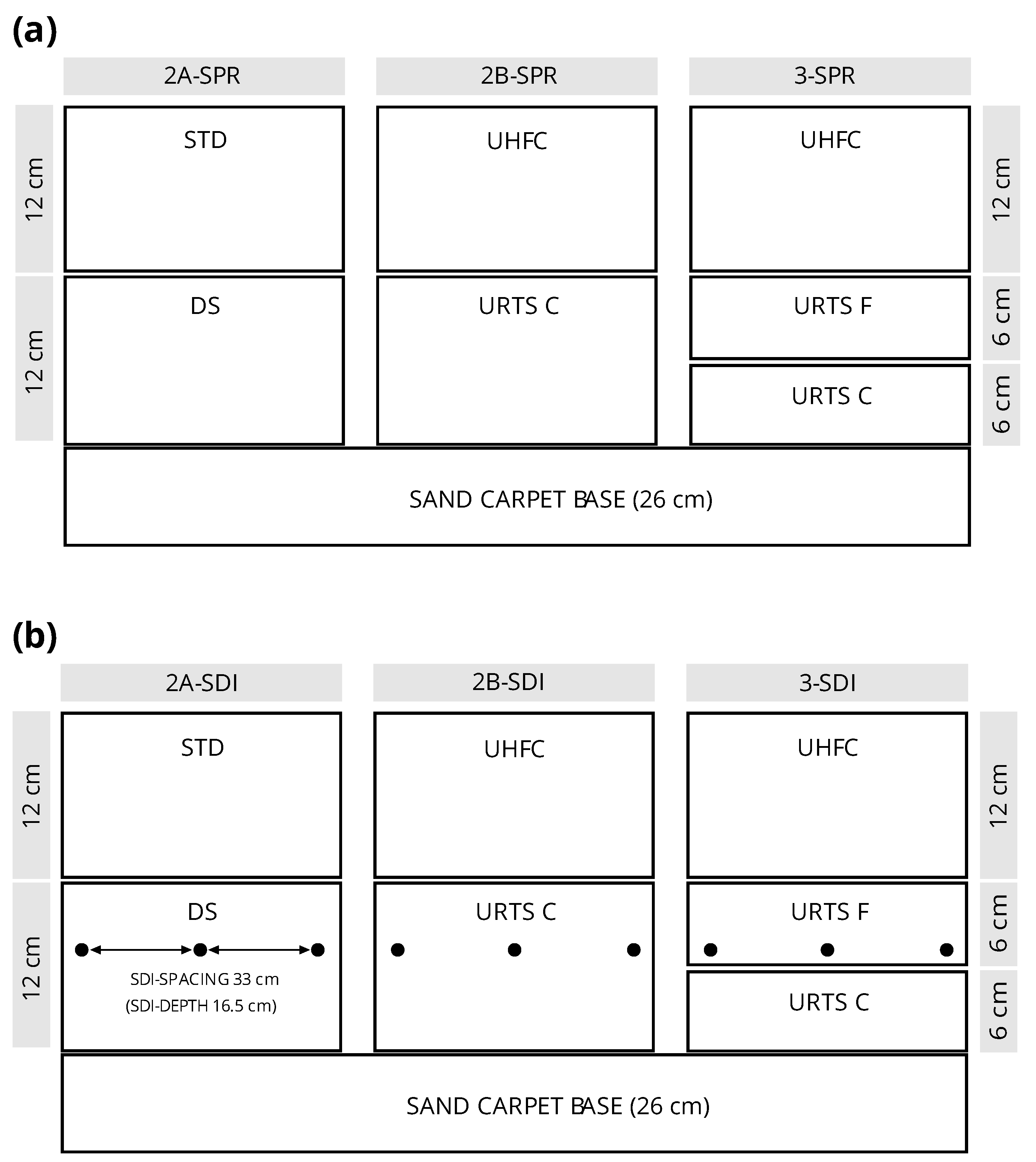
Figure 2.
Triangular grid used for HYDRUS-2D simulations for SDI (left) and sprinkler-irrigated (right) variants and related boundary conditions.
Figure 2.
Triangular grid used for HYDRUS-2D simulations for SDI (left) and sprinkler-irrigated (right) variants and related boundary conditions.
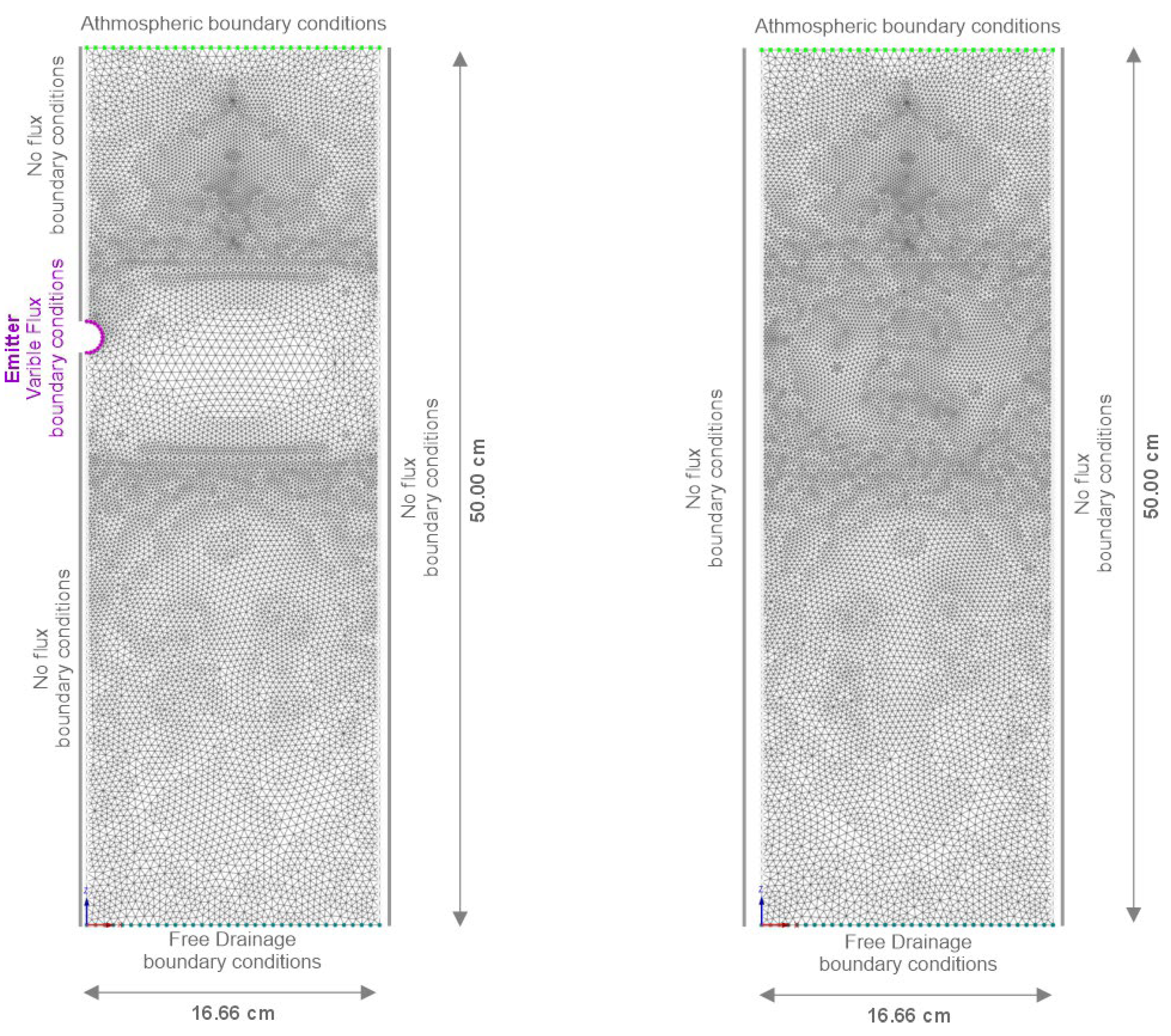
Figure 3.
Volumetric water content within sprinkler-irrigated variants 2A_SPR, 2B_SPR, and 3_SPR at observation depths of 3, 6, and 11 cm (averaged values across the entire observation time 0-48 hours) as observed values (left) and differences between the observed and predicted values (right).
Figure 3.
Volumetric water content within sprinkler-irrigated variants 2A_SPR, 2B_SPR, and 3_SPR at observation depths of 3, 6, and 11 cm (averaged values across the entire observation time 0-48 hours) as observed values (left) and differences between the observed and predicted values (right).
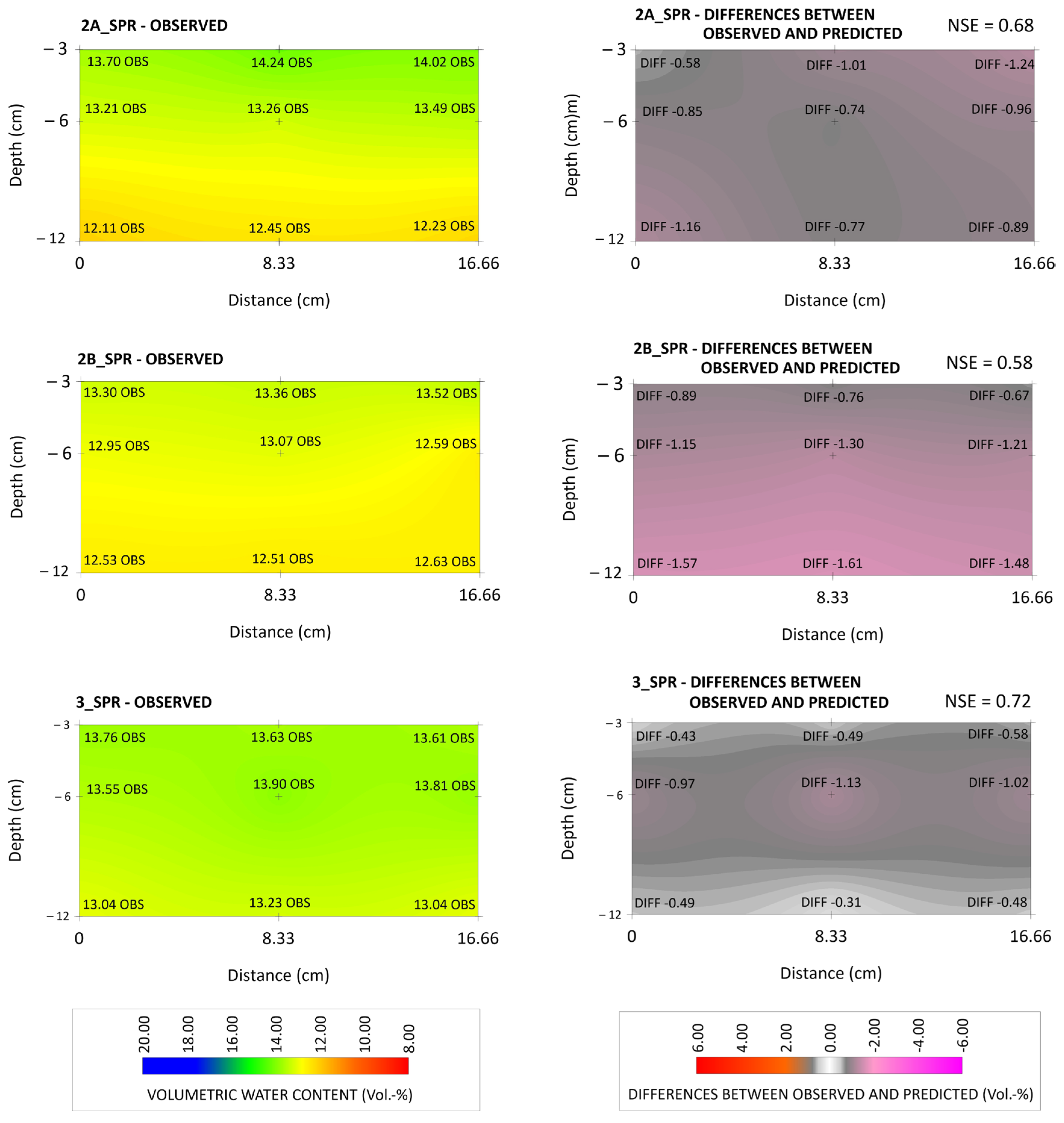
Figure 4.
Volumetric water content within SDI variants 2A_SDI, 2B_SDI, and 3_SDI at observation depths of 3, 6, and 11 cm (averaged values across entire observation time 0-48 hours) as observed values (left) and differences between the observed and predicted values (right).
Figure 4.
Volumetric water content within SDI variants 2A_SDI, 2B_SDI, and 3_SDI at observation depths of 3, 6, and 11 cm (averaged values across entire observation time 0-48 hours) as observed values (left) and differences between the observed and predicted values (right).
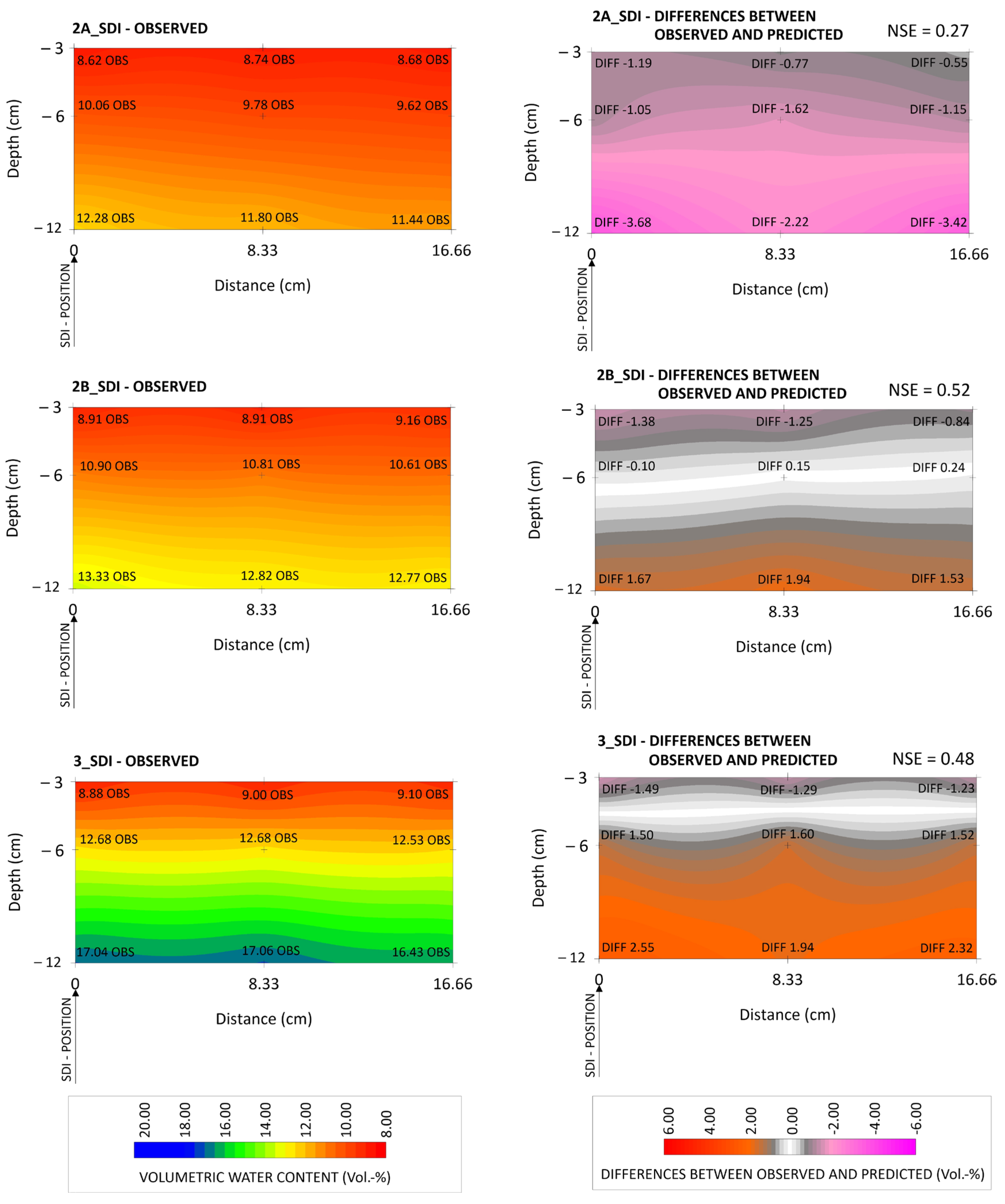
Figure 5.
Influence of a 20% perturbation of soil hydraulic parameters ϴr, n, ϴsw, αw, and α on model efficiency deviation (NSE) across Layer 1 and Layer 2 of the variants (a) 2A_SPR) to (f) 3_SDI during irrigation cycle 1 (10 mm).
Figure 5.
Influence of a 20% perturbation of soil hydraulic parameters ϴr, n, ϴsw, αw, and α on model efficiency deviation (NSE) across Layer 1 and Layer 2 of the variants (a) 2A_SPR) to (f) 3_SDI during irrigation cycle 1 (10 mm).
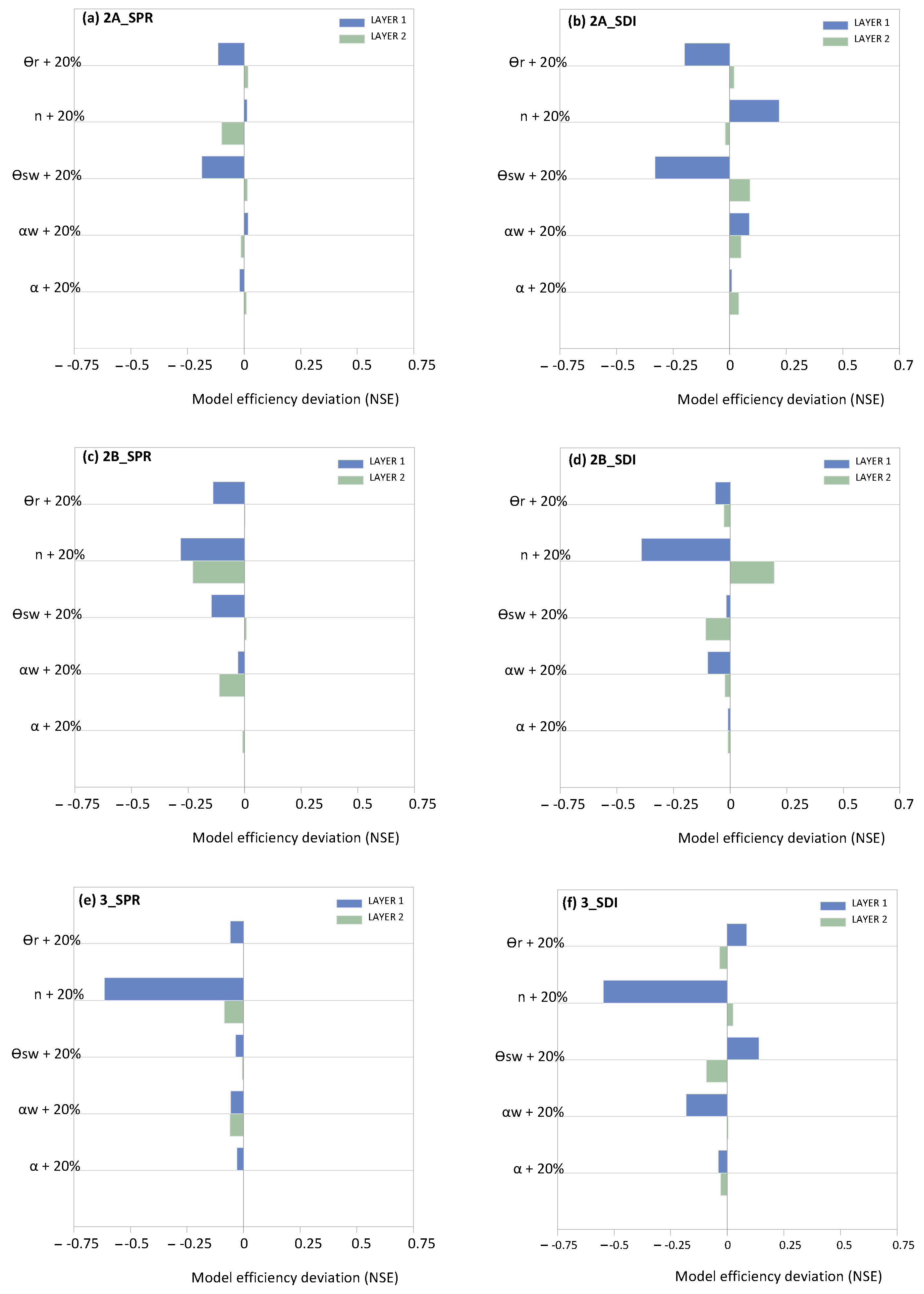
Figure 6.
Development of model efficiency (NSE) under various calibration scenarios (F1–F6) used in isolated implementation (Layer 1 and Layer 2) and combined implementation (Layer 1+2) across variants (a) 2A_SPR to (f) 3_SDI. The red line indicates the model efficiency values under the default settings.
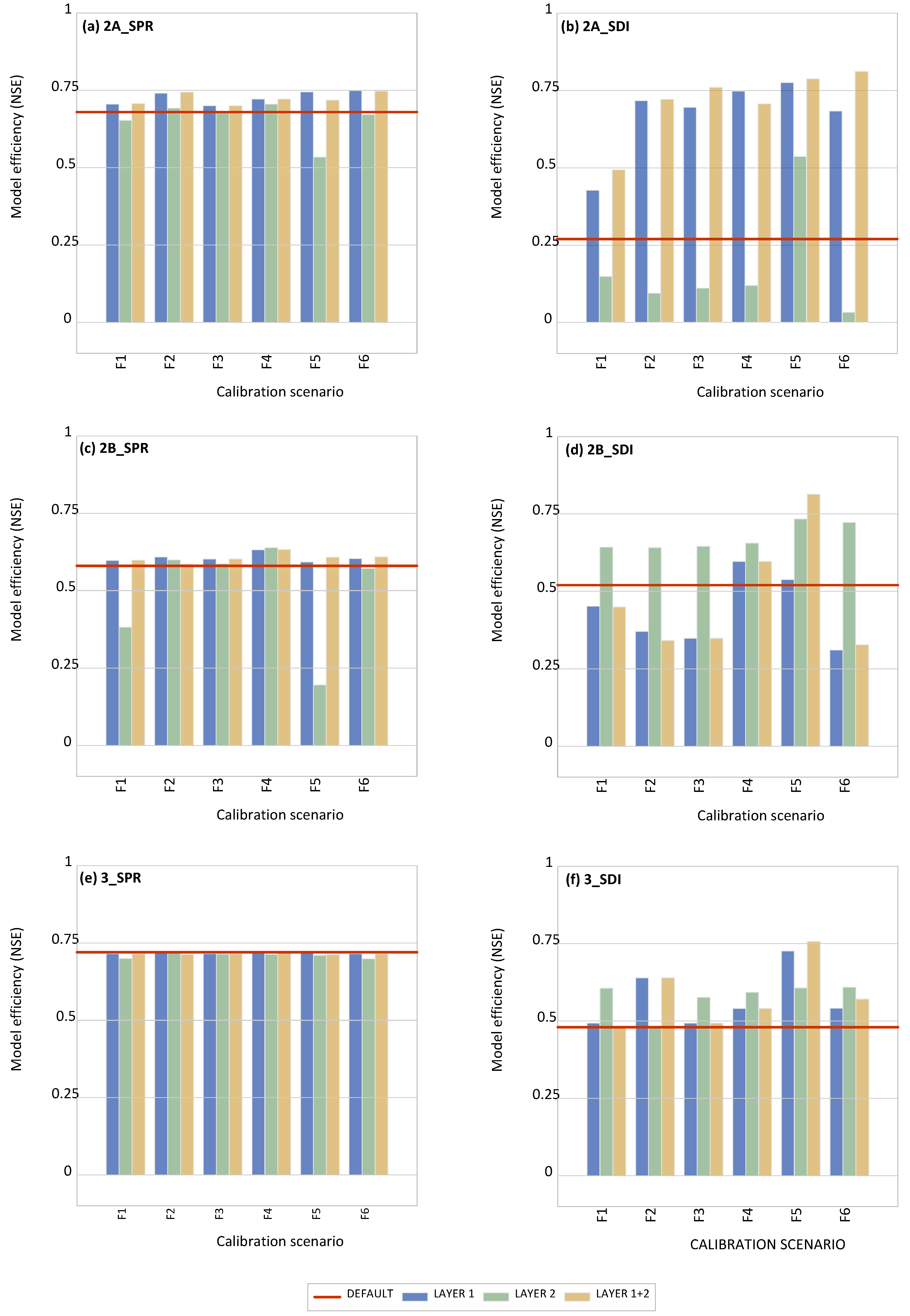
Figure 7.
Measured and predicted volumetric water contents of construction methods 2A, 2B, and 3 under default settings (green line), under SPR irrigation and model calibration scenario F5_L1 (left side, red line and dots), and under SDI and scenario F5_L1+L2 (right side, orange line and dots). R2 refers to the correlation coefficient; significance levels: *** p < 0.001.
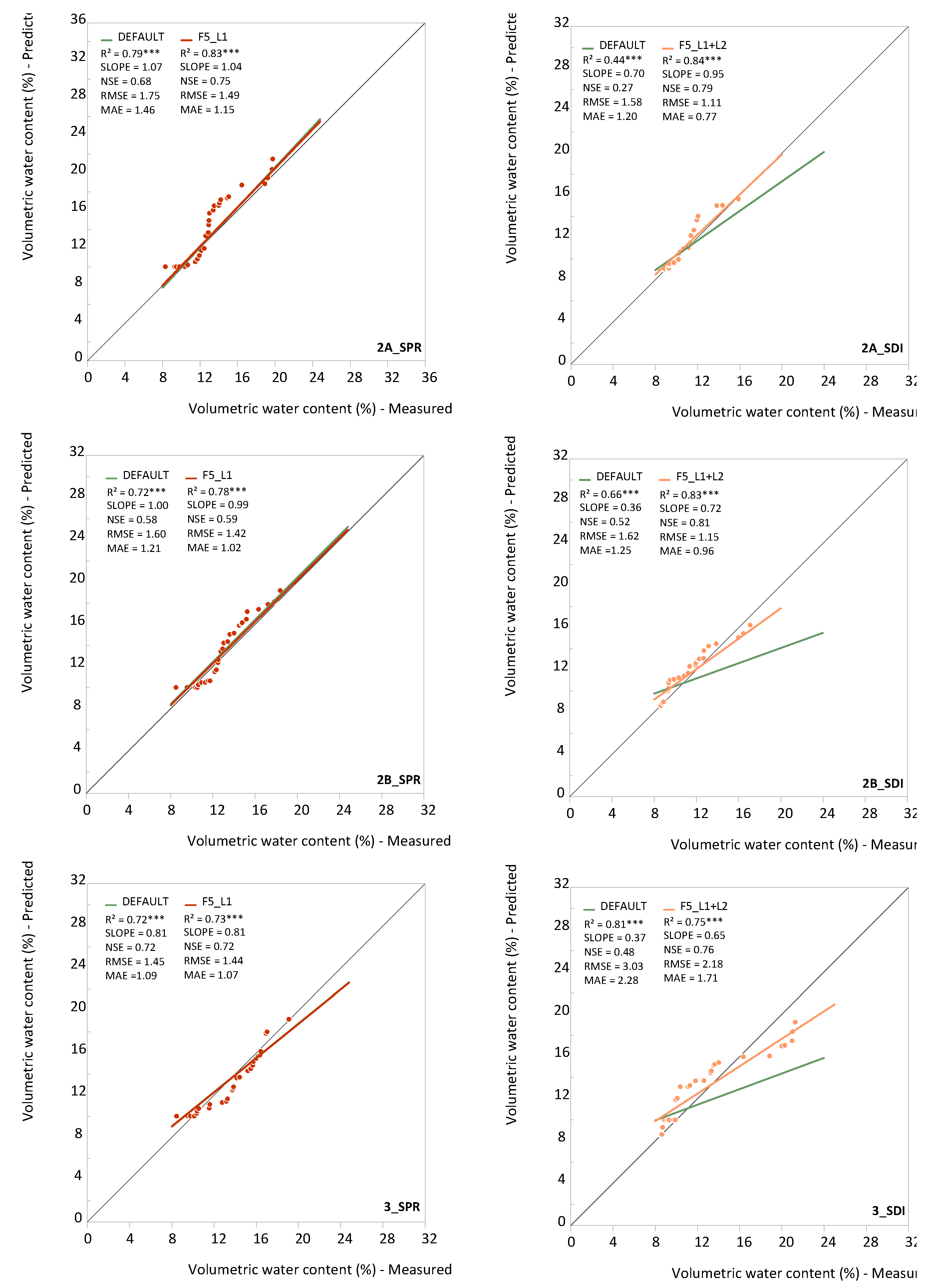
Figure 8.
Development of soil water storage (upper 50 cm) and cumulative drainage flux of the 3-layered construction method 3, irrigation approaches 1–4 under 10 mm SPR, SDI, and hybrid irrigation; observation time: 4, 8, 12, 24, and 48 h after irrigation initiation.
Figure 8.
Development of soil water storage (upper 50 cm) and cumulative drainage flux of the 3-layered construction method 3, irrigation approaches 1–4 under 10 mm SPR, SDI, and hybrid irrigation; observation time: 4, 8, 12, 24, and 48 h after irrigation initiation.


Table 1.
Overview of the five materials used: STD, UHFC (rootzone layer), URTSF (intermediate layer), DS and URTS C (gravel drainage layer) and their associated physical properties.
Table 1.
Overview of the five materials used: STD, UHFC (rootzone layer), URTSF (intermediate layer), DS and URTS C (gravel drainage layer) and their associated physical properties.
| Material | Physical properties | ||||||||
|---|---|---|---|---|---|---|---|---|---|
| Texture* | Grid (mm) | Bulk density (g cm−3) | Ksat (mm h-1)** |
Pore space (% vol.) *** | Field capacity (% vol.) **** | ||||
| Gravel | Sand | Silt | Clay | ||||||
| (% mass) | |||||||||
| STD | (-) | 89.6 | 10.4 | (-) | 0–2 | 1.55 | 220 | 41.5 | 15.9 |
| UHFC | (-) | 98.3 | 1.7 | (-) | 0–2 | 1.46 | 649 | 44.9 | 13.6 |
| URTS F | (-) | 99.6 | 0.4 | (-) | 0.1–0.5 | 1.41 | 1465 | 46.6 | 6.4 |
| DS | 31.5 | 66.1 | 2.4 | (-) | 0–8 | 1.80 | 916 | 32.1 | 6.5 |
| URTS C | (-) | 99.8 | 0.2 | (-) | 0.2–2 | 1.60 | 6081 | 39.6 | 4.6 |
*: Particle size distribution was determined according to [62]. **: Hydraulic conductivity Ksat was determined in the laboratory according to [63]. ***: Pore space was determined from particle density using gas pycnometry [64] and bulk density. ****: Field capacity (at pF 1.8) was determined by hanging a water column in a sand bed according to [65].
Table 2.
Soil parameters in the HYDRUS-2D program.
| Parameters | STD | UHFC | URTSF | URTSC | DS |
|---|---|---|---|---|---|
| ϴs (cm3 cm−3) | 0.415 | 0.430 | 0.466 | 0.394 | 0.321 |
| ϴr (cm3 cm−3) | 0.060 | 0.076 | 0.011 | 0.014 | 0.014 |
| Ks (cm h−1) | 22.019 | 64.854 | 146.474 | 608.12 | 91.612 |
| α | 0.089 | 0.061 | 0.055 | 0.228 | 0.085 |
| αw | 0.118 | 0.119 | 0.077 | 0.300 | 0.156 |
| n | 1.728 | 2.090 | 2.719 | 1.929 | 2.063 |
| l | 0.5 | 0.5 | 0.5 | 0.5 | 0.5 |
Table 3.
Irrigation management parameters within the four irrigation approaches (1-4) under SPR, SDI, and HYBRID (SPR+SDI) irrigation across construction method 3.
Table 3.
Irrigation management parameters within the four irrigation approaches (1-4) under SPR, SDI, and HYBRID (SPR+SDI) irrigation across construction method 3.
| Irrigation approach | Irr. events within 12 h | Water applied per charge (mm) | Proportion | |||||
|---|---|---|---|---|---|---|---|---|
| 0 | 3 | 6 | 9 | 12 | SPR | SDI | ||
| (-) | (-) | hours | (%) | (%) | ||||
| SPR-1 | 1 | 10.00 | 0 | 0 | 0 | 0 | 100 | 0 |
| SPR-2 | 2 | 7.50 | 0 | 2.50 | 0 | 0 | 100 | 0 |
| SPR-3 | 3 | 5.00 | 0 | 2.50 | 0 | 2.50 | 100 | 0 |
| SPR-4 | 4 | 5.00 | 1.25 | 1.25 | 1.25 | 1.25 | 100 | 0 |
| SDI-1 | 1 | 10.00 | 0 | 0 | 0 | 0 | 0 | 100 |
| SDI-2 | 2 | 7.50 | 0 | 2.50 | 0 | 0 | 0 | 100 |
| SDI-3 | 3 | 5.00 | 2.50 | 2.50 | 0 | 100 | ||
| SDI-4 | 4 | 5.00 | 1.25 | 1.25 | 1.25 | 1.25 | 0 | 100 |
| HYBRID-1 | 1 | 5.00 (SPR), 5.00 (SDI) | 0 | 0 | 0 | 0 | 50 | 50 |
| HYBRID-2 | 2 | 7.50 (SPR) | 0 | 2.50 (SDI) | 0 | 0 | 75 | 25 |
| HYBRID-3 | 3 | 5.00 (SPR) | 0 | 2.50 (SDI) | 0 | 2.50 (SDI) | 50 | 50 |
| HYBRID-4 | 4 | 5.00 (SPR) | 1.25 (SDI) | 1.25 (SDI) | 1.25 (SDI) | 1.25 (SDI) | 50 | 50 |
Table 4.
Results of the HYDRUS inverse solution of the van Genuchten parameters within the six model calibration scenarios (F1–F6) for Layer 1 (rootzone STD and UHFC) and Layer 2 (gravel drainage layer DS and intermediate layer URTSF) across the sprinkler- or SDI irrigated construction methods 2A, 2B and 3.
| Layer | Material | *CM | **IS | F1 | F2 | F3 | F4 | F5 | F6 | ||
|---|---|---|---|---|---|---|---|---|---|---|---|
| αw | n | ϴsw | ϴr | αw | n | αw | ϴsw | ||||
| (-) | (cm3 cm−3) | (-) | (-) | (cm3 cm−3) | |||||||
| 1 | STD | 2A | SPR | 0.147 | 1.842 | 0.402 | 0.056 | 0.144 | 1.833 | 0.164 | 0.382 |
| SDI | 0.152 | 2.076 | 0.306 | 0.035 | 0.109 | 2.095 | 0.145 | 0.311 | |||
| UHFC | 2B | SPR | 0.127 | 2.153 | 0.420 | 0.073 | 0.131 | 2.052 | 0.131 | 0.430 | |
| SDI | 0.136 | 2.306 | 0.322 | 0.058 | 0.117 | 2.110 | 0.128 | 0.329 | |||
| 3 | SPR | 0.119 | 2.080 | 0.430 | 0.076 | 0.119 | 2.084 | 0.119 | 0.430 | ||
| SDI | 0.119 | 1.905 | 0,430 | 0.074 | 0,121 | 1,826 | 0.103 | 0,430 | |||
| 2 | DS | 2A | SPR | 0.152 | 1.983 | 0.321 | 0.013 | 0.203 | 1.764 | 0.166 | 0.321 |
| SDI | 0.388 | 2.076 | 0.240 | 0.011 | 0.207 | 3.005 | 0.207 | 0.241 | |||
| 2B | SPR | 0.129 | 1.881 | 0.321 | 0.022 | 0.116 | 2.199 | 0.097 | 0.121 | ||
| SDI | 0.155 | 2.042 | 0.321 | 0.014 | 0.202 | 2.332 | 0.154 | 0.321 | |||
| URTSF | 3 | SPR | 0.076 | 2.662 | 0.466 | 0.023 | 0.077 | 2.671 | 0.077 | 0.466 | |
| SDI | 0.083 | 2.719 | 0.466 | 0.011 | 0.079 | 2.720 | 0.087 | 0.466 | |||
| NOTE. | |||||||||||
| * Construction method | |||||||||||
| ** Irrigation system | |||||||||||
Disclaimer/Publisher’s Note: The statements, opinions and data contained in all publications are solely those of the individual author(s) and contributor(s) and not of MDPI and/or the editor(s). MDPI and/or the editor(s) disclaim responsibility for any injury to people or property resulting from any ideas, methods, instructions or products referred to in the content. |
© 2025 by the authors. Licensee MDPI, Basel, Switzerland. This article is an open access article distributed under the terms and conditions of the Creative Commons Attribution (CC BY) license (http://creativecommons.org/licenses/by/4.0/).
Copyright: This open access article is published under a Creative Commons CC BY 4.0 license, which permit the free download, distribution, and reuse, provided that the author and preprint are cited in any reuse.


