Submitted:
12 January 2025
Posted:
13 January 2025
You are already at the latest version
Abstract
Modern manufacturing enterprises face many challenges that have to be overcome to keep the operation sustainable and effective. Among the key issues, one may mention the stiction of control valves that may cause inefficiency in process operations, increased energy consumption, and disturbed production stability. This article is devoted to exploring a sinusoidal compensation method in order to address stiction challenges. The proposed methodology will contribute to enhancing industrial process sustainability by reducing oscillatory behavior in manufacturing systems, hence assuring smooth operations with minimal environmental impact.
Keywords:
sustainable manufacturing
; valve stiction
; process optimization
; energy efficiency
; sinusoidal compensation
; production stability
1. Introduction
Control systems in manufacturing, especially in maintaining product quality and operational efficiency, have a vital role. The nonlinearities in valve movement cause stiction, a condition that has an adverse effect on process sustainability by wasting more resources and reducing profitability. By addressing stiction, enterprise efficiency will be improved and sustainable manufacturing enhanced with better use of energy and materials. The present study investigates a sinusoidal compensation method and presents it as a sustainable solution for the industrial manufacturing enterprise control valve stiction problem.
Valve stiction usually is modeled as a sum of static and dynamic frictions. The most usually applied LuGre friction model and other empirical models mathematically represent the stiction. A very simplified representation of the behavior of valve stiction may be described as:
Where:
- f(t): Friction force at time tt.
- Fs: Static friction (force required to overcome stiction).
- Fc: Dynamic (kinetic) friction.
- v(t): Velocity of the valve stem.
- x(t): Displacement of the valve stem.
- xstick: Threshold displacement for stiction.
This equation reflects friction force dependence on either sticking or moving of a valve, where friction is larger under static conditions. ISA defines stiction as the resistance to the start of motion, usually measured as the difference between the driving values required to overcome the static friction upscale and downscale.
Indeed, from a study of real process data, it is observed that the phase-plane portrait of a valve input vs. output response can be characterized as, for a sticky valve, Figure 1: It comprises a deadband, stick band, slip jump, and a moving phase: when the valve comes to a rest or changes direction to 'A point,' the valve sticks. Once the controller output overcomes the dead band 'AB' plus the stick bank 'BC' of the valve, the valve jumps to a new position 'point D' and continues to move. The deadband and stickband represent the behavior of the valve when it is not moving even though the input to the valve is changing. The slip jump represents the sudden release of potential energy stored in the actual chamber as kinetic energy due to high static friction as the valve starts to move. Once the valve moves, it continues to move until it sticks again at point E.
There are two loops simulated under closed loop, which are a concentration loop and a level loop. The concentration loop has slow dynamics with large dead time, while that for the level loop only has an integrator. The transfer function obtained from Horch and Isaksson, 1998, along with the stiction model, was used for its simulation. Since it is known that the presence of pure deadband or backlash does not form a limit cycle, but, in contrast, it only adds dead time to the process, while that for deadband with an integrator produces a limit cycle. It is not advisable to plot valve position (mv) against (pv) if the data for valve position is available; instead, plot valve position (mv) against controller output (op) since this particular plot only shows some kind of elliptical loops with sharp turnaround points. Level loop was investigated using only an integrator for the typical behavior of the process in the presence of valve stiction. From the simulation, it follows that the presence of a pure dead band is enough to cause oscillations. A pure dead band, hence, can create limit cycles by adding an integrator in the process, or the cycle otherwise will decay to zero. The same kind of PV-OP plots of elliptical loops with sharp turnarounds is obtained from simulation (Choudhury et al., 2005).
2. Literature Review
Stiction in control systems has been a subject of research due to its pervasive impact on manufacturing enterprises. Previous studies have looked into various methods, including pulse-based and model-free compensation techniques (Choudhury et al., 2005; Farenzena & Trierweiler, 2007; Hagglund, 2002; Hassan, 2015; Lakshminarayanan, 2009; Srinivasan & Rengaswamy, 2008). However, most of these methods tend to increase the wear and energy consumption of the system. The sinusoidal compensation method proposed in this paper extends previous works by introducing a sustainable approach with smoother valve movements and less variation. Some of the most relevant findings from previous works are:
- Pulse Compensation: Effective in eliminating oscillations but causes rapid wear on valves, hence not sustainable for long.
- Tuning Proportional-Integral (PI) Controllers: Mitigates stiction but at the cost of increased steady-state errors.
- Sinusoidal Compensation: Demonstrated to offer optimal results in reducing oscillatory behaviors with minimal energy use and system stress.
Thus, sustainable practice integration within manufacturing enterprises has become a high priority for addressing operating-related inefficiencies. Of these various losses, stiction of control valves results in oscillatory behavior in industrial systems; this causes a lot of resource wastage with a greater ecological footprint. Hence, efficient stiction compensation methods contribute significantly to sustainable manufacturing and enterprise optimization. It is a review that reflects on prevailing methods and their limitations while introducing sinusoidal compensation as an effective alternative. Horch (2000) observed that stiction affects the control loop performance as well as accelerates wear and tear of valves, hence causing the reduction in the lifecycle of the valve (Horch, 2000; Horch & Isaksson, 1998).
Different approaches have been advanced to eradicate stiction in the control valve with various levels of success. One such approach, known as pulse compensation, put forward by Hagglund (2002), implements small periodic pulses to surmount static friction. This approach, however, is found to dampen oscillations but again was faced by criticism with regards to the aggressiveness of the stem movements when it resulted in rapid valve wear. It is also a computationally expensive process since it involves the tuning of several pulse parameters (Hagglund, 2002).
PI controller tuning was prevalent among the approaches used to compensate for stiction; under this technique, an appropriate tuning of the controller gain and reset time results in reducing the amplitude of oscillations. (Ruel, 2000). However, studies have shown that PI tuning may introduce steady-state errors and increase the frequency of limit cycles, compromising system efficiency (Farenzena & Trierweiler, 2007).
Model-free methods have attracted interest due to their dynamic adaptability without a precise model of the control system. Examples include constant reinforcement (CR) methods, which inject a compensating signal into the valve to maintain the movement (Ruel, 2000). In addition, most of them cannot effectively handle severe stiction cases.
Optimization methods seek an optimum set of parameters for compensation using mathematical models. Canudas de Wit et al. (1995) worked on developing an optimization framework based on stiction severity estimation. While this method attains precision, it is also restricted by computational inefficiencies and the possibility of local minima, especially in complex industrial systems, as in (de Wit et al., 1995).
The sinusoidal compensation method addresses the limitations of existing techniques by introducing a non-aggressive compensating signal that reduces variability and energy use. According to (Choudhury et al., 2005), this method minimizes valve wear by employing sinusoidal waves characterized by fundamental frequencies, eliminating the harmonics that cause sudden valve movements in pulse-based methods. Furthermore, the sinusoidal approach has exhibited superior performance in reducing ISE values at various stiction severities and, thus, can be a robust choice for sustainable manufacturing operations.
Wu et al. (2020) discussed the dynamic nature of stiction and its influence on process stability, underlining the need for advanced compensation methods in sustainable manufacturing conditions (Wu et al., 2020).
Several advanced methods have been developed recently to address stiction. Recent works apply machine learning for predictive stiction management, such as in (Di Capaci et al., 2020; Di Capaci & Scali, 2016).To illustrate this, Di Capaci et al. present a cloud-based monitoring approach that integrates data analytics into predictive algorithms for the mitigation of stiction. This fully meets the objectives of Industry 4.0 and helps in enhancing sustainability by the reduction of process disruptions. (Wu et al., 2020) performed a critical review of dynamic modeling approaches for stiction; this helps reduce oscillation and consequently enhances energy efficiency. These models allow very accurate predictions and real-time adjustments that support sustainable operations. Sinusoidal compensation remains one of the robust approaches to reducing valve wear and oscillatory behavior. Recent studies, such as (Bascur, 2019), have validated its efficacy in the improvement of process control stability while conserving energy and material. Stiction detection has also been introduced with integrated systems for condition monitoring and control optimization. For instance, in the work of (Vallati & Anastasi, 2020), a technological demonstrator for cloud-based performance monitoring is presented, allowing real-time diagnostics while answering sustainability goals.
Among them, machine learning-based techniques have excellent adaptability and predictive performance but involve huge computational resources. Dynamic modeling would imply a too complex implementation in an industrial manufacturing scenario. Sinusoidal compensation is a very simple and effective solution to be applied in a variety of manufacturing situations. Integrated systems allow thorough monitoring but depend on the availability of adequate infrastructure.
The contribution of reviewed methods refers to the scope of operational inefficiency, as well as to wider sustainability goals due to optimized resource use and minimized emissions. In (Di Capaci et al., 2020), predictive analytics highlighted their potential for waste minimization, while Wu et al. (2020) underlined the dynamic model in terms of energy saving. This section summarizes different methods applied for stiction compensation in control valves (Wu et al., 2020).
2.1. Summary Table of Compensation Methods
Below is the comprehensive summary table, including the equations commonly used for each stiction compensation method:

Table 1.
Summary table of Valve Stiction Compensation Methods.
| Method | Principle | Equation | Advantages | Limitations |
|---|---|---|---|---|
| Pulse-Based | High-frequency pulses | Effective for extreme stiction | Rapid wear and high energy cost | |
| Sinusoidal Compensation | Smooth sinusoidal inputs | Energy-efficient, reduces wear | Requires tuning | |
| PID Tuning | Adjusting controller gains | Simple to implement | Risk of steady-state errors | |
| Model-Based Compensation | Friction modeling |
|
x(t) | Computational complexity |
| Machine Learning | Predictive algorithms | Robust and adaptive | High computational demand | |
| Constant Reinforcement | Small constant input bias | Simple and cost-effective | Higher energy usage | |
| Optimization-Based | Algorithmic input optimization | Maximize the objective function by minmizing the error | u(t) | Computationally intensive |
Where for the Pulse Method, u(t): Control input signal, Ap: Amplitude of the pulse signal, ωp: Frequency of the pulse.
For the Sinusoidal Compensation, ucontrol: Original control input signal, As: Amplitude of the sinusoidal signal, ωs: Frequency of the sinusoidal signal.
For the PID tuning, e(t) is the error signal, and Kp, Ki, and Kd are the proportional, integral, and derivative gains, respectively.
For the model-based compensation, f(t) is the friction force. Fs: Static friction, Fc: Dynamic friction, x(t): Valve stem displacement.
For the machine learning-based compensation, predict u(t) using trained models fML, where inputs include historical data such as valve position (xt) and velocity (vt).
For the constant reinforcement, B: Constant bias is added to the control signal to prevent static conditions.
2.2. Causes and Characteristics of Valve Stiction
Valve stiction is caused by static friction that prevents the valve from responding promptly to actuator signals, leading to oscillatory behavior and inefficiencies.
- Horch and Isaksson (1998) highlighted that valve stiction results in uneven responses to control signals, particularly under high-pressure conditions, which disrupts process stability and increases energy demands (Horch & Isaksson, 1998).
- Lakshminarayanan (2009) proposed a unified approach for quantifying stiction, noting its strong correlation with valve wear and process disruptions (Lakshminarayanan, 2009).
2.3. Impacts on Energy Consumption
The energy implications of valve stiction are multifaceted, including increased actuator workload, prolonged stabilization periods, and process inefficiencies:
- Kano and Maruta (2004) emphasized that stiction leads to excessive actuator movements, which, in turn, cause significant energy losses during frequent corrections (Kano & Maruta, 2004).
- Daneshwar and Noh (2014) developed fuzzy system models to analyze stiction-induced energy consumption, demonstrating that systems with unaddressed stiction used up to 30% more energy compared to compensated systems (Daneshwar & Noh, 2014).
2.4. Detection and Diagnosis Techniques
Early detection of stiction is essential to reduce energy consumption and maintain the reliability of the system.
- Preprocessing techniques for early stiction detection using AI were proposed at industrial setups with improved diagnostic accuracy (Navada & Sravani, 2024).
- Mathur et al. (2020) established a correlation between stiction and control valve lifecycle prediction while highlighting the evaluation of detection algorithms in minimizing maintenance and energy costs (Mathur et al., 2020).
2.5. Compensation and Mitigation Strategies
Compensation techniques that address energy losses due to valve stiction:
- Di Capaci and Scali (2016) investigated system identification methodologies for quantifying stiction and showed a significant contribution of adaptive compliance in reducing energy waste (Di Capaci & Scali, 2016).
- Garrido et al. (2023) explored cost-effective compensation strategies for electric valves, demonstrating significant energy savings with optimized valve actuation paths and diminished oscillations (Garrido et al., 2023).
2.6. Impacts on Maintenance and Operational Costs
Stiction causes not just energy waste but increases wear and maintenance requirements on the valve.
- The oscillations caused by stiction increase valve movement and consequently wear, raising maintenance costs by as much as 40% (Srinivasan & Rengaswamy, 2008).
- Hassan (2015) presented pneumatic compensation methods, which prolong the lifetime of valves by mitigating wear (Hassan, 2015).
2.7. Advanced Modeling Approaches
Recent improvements in modeling techniques offer more insights into the dynamics of stiction. Stiction model integration into energy optimization frameworks was suggested as a factor that can be effectively used to quantify energy savings. Lakshminarayanan (2009) emphasized the importance of integrating stiction models into energy optimization frameworks, demonstrating their effectiveness in quantifying energy savings (Lakshminarayanan, 2009). Practical models to forecast the effects of stiction on industrial systems were developed by Kano and Maruta (2004), enabling predictive maintenance and energy-efficient operations (Kano & Maruta, 2004).
Collectively, these reviewed studies demonstrated that valve stiction can enhance energy usage, ongoing costs, and repair requirements. Proposed detection and compensation techniques by (Navada & Sravani, 2024) and (Di Capaci & Scali, 2016) can help mitigate these effects. Abundant energy savings and process reliability improvements can be achieved through the integration of advanced diagnostic tools and compensation algorithm capabilities into industrial systems.
3. Methodology
In this study, three methods of compensation were selected, namely the pulse, sinusoidal, and PID tuning methods. The tuning parameters are changed for PID tuning to reduce the error between the output signal and the setpoint. For the pulse and sinusoidal method, valve movements are optimized by calculated frequencies and amplitudes. To assess the performance in mild, moderate, and severe stiction scenarios, MATLAB simulations based on different stiction conditions were conducted. The main criteria were the rise time, settling time, and integral squared error (ISE).
3.1. Valve Stiction Model
The valve stiction model that involves different scenarios of stiction is developed in the MATLAB/Simulink environment. A control valve model incorporating static and dynamic friction elements is developed to emulate real-world stiction behavior. Choudhury’s model (see Figure 2) was the model used to demonstrate the dynamics of the valve stiction (Choudhury et al., 2005; Kano & Maruta, 2004). The selected process reflects the dynamics of the change in concentration in a tank. For the closed-loop dynamics, the valve output obeys a first order with dead time response (Eq. (2)), while the controller represents a PI controller (Eq. (3)).
The system runs in the discrete domain, and the transfer function that represents the system is:
In this paper, step time is chosen at 1000 units for getting the change of response more clear, and the program was simulated for 10,000 units. The condition given for choosing the sampling time (Ts) is given in the literature to be less than or equal to 1. It is chosen to be 0.1 to obtain good responses. The initial value for step change is at 0, and the final value is at 10. The compensation methods are tested with various conditions of stiction parameters that are calculated and shown in the results sections. This is done through analyzing the variables, where ranges were obtained using the DoE methodology. The initial ranges in literature for S and J were identified to be 1-10 and 0-1, respectively (Di Capaci & Scali, 2016; Lakshminarayanan, 2009).
The compensation algorithms are developed and used to test the valve stiction model. The PID controller is added and tuned to obtain the best performance. Regarding the sinusoidal compensation algorithm, this is designed in a systematic manner, where initially the user injects low-amplitude sinusoidal signals into the valve input to counteract stiction effects. The methodology for designing the compensation algorithm includes signal design, phase adjustment, and integration with the control loop. The signal design frequency is determined based on the dominant frequency of oscillations in the control loop. The amplitude is calibrated to overcome static friction without inducing excessive valve movements. The phase adjustment ensures the sinusoidal signal is aligned with the control signal, hence maximizing the effectiveness of compensation. Regarding integration, the sinusoidal signal is added to the controller’s output, creating a composite input that minimizes stiction-induced nonlinearity.
The model is subjected to different levels of stiction severity: mild, moderate, and severe. The sinusoidal compensation method is integrated with a proportional-integral-derivative (PID) controller, a widely used control scheme in industrial processes. The identification of the severity depends on the values of slip and jump, represented as slip-up (SU), slip-down (SD), and jump (J). The suggested values from literature ranges for S and J are 1-10 and 0-1, respectively (Choudhury et al., 2005; Kano & Maruta, 2004). Due to the different ranges, the possibilities of the number of severity simulation tests would be very high. For this reason, the design of experiments will be part of the methodology to identify the most effective valve stiction severities.
For PID tuning, the ranges of Kc values are also identified using the root locus method to ensure stability. Kc values were found to range between 34.3 and 0.165. The range for τi was initially difficult to find. An approximation was done to decrease the order of the closed-loop transfer function from 5th order to 2nd to make it fit well with the complex process. Swamy’s approximation was used to get the time delay, while Smith approximation gave acceptable data for ξ and τ [16]. The approximations were used for ease in the Routh stability calculation and for later use in Direct Synthesis (DS) and Internal Model Control (IMC) tuning methods. The approximated transfer function is.
A new approach for the Routh stability was considered to calculate the range for τi using the values of Kc (34.3 and 0.165). Each Kc value yielded slightly different values, yet an acceptable range for τi was 0.005 to 0.184. Table (3-1) shows the maximum and minimum for each variable.
As stated earlier, the design of experiments (DoE) was implemented. The range of S was divided into 3 values (1, 5, and 10), and the range of J was divided into 2 (0 and 1) for experimenting. This leaves us with 6 experiments to perform.
The performance of the methodology is evaluated using the following metrics:
• Rise Time: The time taken by the process variable to go from a lower value to the setpoint following a disturbance.
• Settling Time: The time taken by the process variable to stay within a tight error interval.
• Energy Consumption: The energy used by the actuator during valve operation.
• Valve Travel: The total amount of valve movement over the duration of the simulation, which acts as a proxy for wear and tear.
Table 2.
Ranges of the four variables.
| Variable | Maximum | Minimum |
|---|---|---|
| 34.3 | 0.165 | |
| 0.184 | 0.005 | |
| S | 10 | 1 |
| J | 1 | 0 |
Additional important measurements include oscillation amplitude, the integral of squared error (ISE), and valve travel, which describes the frequency and amplitude of valve excursions that suggest wear and tear edge deterioration.
The proposed validated sinusoidal compensation method has been applied to a practical industrial process to verify its effectiveness. The collected data from sensors and control systems are used to determine if the appropriate ability to support different stiction levels and process dynamics is achieved. Calculations are made of the reductions in energy use, emissions, and maintenance requirements.
3.2. Basis for Calculating Energy Consumption and Maintenance Costs Related to Valve Stiction
Using a systematic approach, the impact of valve stiction on energy consumption, maintenance expenses, and process efficiency—considering wear-out, oscillatory reactions, and operational inefficiencies—is also evaluated.
3.2.1. Energy Consumption due to Valve Stiction
These parameters have different effects on energy consumption, but in general, stiction leads to the need for excess energy to initiate motion and can occasionally result in out-of-control situations. The following are identified as contributing factors:
Valve Travel Distance (DD):
Increased valve movements due to stiction result in higher energy use by the actuator.
Where:
- ○
- Xi: Valve displacement at time ii.
- ○
- N: Total number of control actions.
Actuator Power Requirement (PP):
The power needed to move the valve is proportional to the resistance (friction) and travel distance:
Where:
- ○
- F: Frictional force (dependent on stiction severity).
- ○
- v: Velocity of valve movement.
- ○
- k1, k2: Constants based on actuator efficiency and load.
Energy Consumption (EE):
Total energy used over a period is:
Where T is the operation time.
This can have an impact for the following reasons:
• Oscillatory responses lead to increased valve travel, which raises energy consumption.
• Techniques like sinusoidal inputs can be used to mitigate unnecessary valve motion, thereby saving energy.
3.2.2. Maintenance Costs Due to Wear and Tear
Stiction increases wear and tear on valves and actuators, leading to higher maintenance costs. The key factors are:
Valve Wear (W):
Wear is proportional to the cumulative valve travel and frictional force:
Where:
- ○
- α: Wear coefficient (material-dependent).
Frequency of Repairs (R):
Repair frequency depends on wear rate and operating conditions:
Maintenance Costs (Cm):
Total cost over a period includes repair costs and downtime:
Where:
- ○
- Cr: Cost per repair.
- ○
- Td: Downtime due to repairs.
- ○
- Co: Opportunity cost (lost production).
The implications of this will play out in the following way:
- Stiction-induced oscillatory responses raise D, F, and W, resulting in more repairs.
- Smooth compensation methods can optimize valve movement and reduce friction, making maintenance more cost-effective.
3.2.3. Costs Due to Product Variations
Stiction-induced oscillations in control systems can lead to variations in product quality, increasing operational costs. The key factors are:
Deviation in Process Variables (σ):
Oscillatory responses cause deviations in critical variables (e.g., temperature, pressure):
Where:
- ○
- y(t): Measured process variable.
- ○
- ysetpoint: Desired value.
Rework or Scrap Costs (Cs):
Higher deviations lead to more rework or scrap:
Where β is a proportionality constant based on the cost of deviation.
Increased Utility Costs (Cu):
Oscillations often result in inefficient use of utilities (e.g., heating, cooling):
Where ΔU(t): Excess utility usage due to oscillations.
It will be impacted due to these reasons:
• Stiction accounts for increased variability (σ), which raises costs associated with rework, scrap, and utility usage.
• Better control, reducing oscillations, dramatically reduces those costs.
3.2.4. Total Cost Model
The total cost associated with valve stiction can be summarized as:
Where:
- Ce: Energy costs (EE).
- Cm: Maintenance costs.
- Cq: Quality-related costs (rework, scrap, utilities).
Results concerning cost, efficiency, and energy consumption will be displayed using the best compensation method, depicting its effects before and after the compensation process. This is reflected in reduced valve motion—smooth sinusoidal inputs prevent unnecessary valve movements, thereby reducing D and W. Additionally, this is measured through lower energy consumption, as reduced valve oscillations decrease energy (E) usage. Finally, as the system stabilizes over time, variance in valve movement is minimized, producing a stable process with reduced σ, leading to lower rework and utility costs.
4. Results and Discussion
A modified version of the two-parameter data-driven stiction model developed by Shoukat Choudhury is used for simulation. The response is analyzed with properties such as rise time, overshoot, and settling time. Figure 3 represents the block diagram of a closed-loop control system (closed control loop) in the presence of stiction with the addition of a stiction compensator in the valve. Valve dynamics can be observed only after the stem movement to analyze how it changes to create non-linearity. The compensator can be successfully used to minimize the stiction-induced oscillation from process output. Stream 1 is the output of process set-point, which is from step block {set in step block}. Stream 2 represents the error (set point – process variable), which is the input to the PI controller. Stream 3 is the output from the PI controller, OP is the saturation output, Stream 4 is the compensator output, and a sine wave is used as a compensator, which is proposed as a compensating method using a sinusoidal signal. The valve stiction compensator is inserted between the saturation and the valve movement. Stream 5 is the additive signal (OP + stream 4) that is being fed to the valve. MV is represented as the change in the stem position obtained using the stiction model. PV is the output of a process that is represented as the discrete transfer function. PV1 is the additive signal of PV process output, and stream 6 highlights the random number output as a disturbance in the closed control loop. PV1 process output is added to the signal with stream 7, which is the process set point. Stream 8 and stream 9 represent the ISE.
The three identified compensation methods were implemented:
1) Pulse method 2) Sinusoidal method 3) Controller tuned as compensator.
4.1. Design of Experiments
Analyzing the variables was done through the Design of Experiment (DoE) option in MINITAB. The results of the DoE were calculated. The interactions are studied to identify the main effect.
Figure 4 shows the main effect of each variable on the output. It is obvious that the Kc has the highest effect, followed by the τi . This is analyzed by observing that Kc is steeper; it will have a higher effect on the output. Moreover, J and S affect the output in opposite manners. If decreasing S will decrease the output, decreasing J will do the opposite. When j=0, the valve won’t open at all. It will stay in its stick position for a long while, which explains the high amount of stiction.
Figure 5 shows the interaction of variables with each other. S and J have the best interaction, which means that they affect each other’s results and may affect the output significantly but in an inversed way. On one hand, S's relation with Kc is minimal since they won’t interact at all, but there is a slight effect of τi on S. On the other hand, since J has the opposite relation with S, Kc has a slight interaction while τi has minimal effect.
4.2. Quantification
The PV-OP plot is used to diagnose the type of non-linearity; thus, the plot will show the elliptical patterns indicating valve stiction (Di Capaci & Scali, 2016; Lakshminarayanan, 2009). To measure stiction, the previously used clustering technique was selected due to its simplicity and accuracy. Without a time delay, the stiction amount was determined to be 11.25%. Additionally, an apparent stiction of 13.2% was calculated with a time delay.
As real-world data comes with noise and disturbances, the Wiener filter was introduced. The PV-OP graph generally lacks clear meaning, making it necessary to clean the data for clearer results. This filter is a stationary linear filter optimized for images corrupted by both additive noise and blurring. Both PV and OP signals were checked for any significant peaks and filtered accordingly. The Wiener filter applies a pixel-wise adaptive low-pass approach to grayscale images. The Wiener filter produced a clean, clear plot, initiating the quantification process. To compare stiction amounts, it was crucial to establish a single definition. High stiction was defined as the most problematic scenario for the process, occurring when S = 10 and J = 0, as described. The area under the curve was calculated from the plot design for varying values of S and J. These values were not randomly selected; rather, the ranges of both parameters were divided into three sections for a more systematic evaluation. S ranged from 0 to 10, while J was adjusted between 0 and 1.
Stiction classification was based on dividing the area into three categories, as stiction is directly proportional to the area. Greater stiction in the valve corresponds to smaller area values and greater distance between the S and J parameters. Values above 37.67 were classified as high stiction, values above 18.84 were classified as mild stiction, and values above 0 were classified as low stiction.
Figure (5) and Table (3) show a clearer comparison proving that S and J provide oppositive effects as explained in the design of the experiment section previously. Table 3 shows the stiction area of the six experiments.
After the stages of identifying the stiction parameters based on the design of experiments and quantification, the next step is to tune the PID controller before finally applying the compensation methods.
4.3. Compensation Using Kc and τi Tuning
The tuning methods used are obtained using internal model control (IMC) and direct synthesis (DS) methods. Both methods oddly yielded the same results for Kc and τi. The obtained tuned controller contained a derivative part, and it was ignored due to the incredibly small effect of it. The tuning parameters were identified as shown in Table 4. As the table shows, since τi is related to J, and since J was not changing significantly, τi was not changed. On the other hand, since Kc was changed with every change of S, which shows that their interaction is bigger than that of J and τi.
4.4. Simulation Results
The difference between the compensated and uncompensated output is shown in Figure 6. The uncompensated output exhibits regular high peaks, which are indicative of stiction. After tuning and applying the compensation method, the stiction was eliminated.
A simulated control loop was used to evaluate the sinusoidal compensation method across three scenarios: mild, moderate, and severe stiction. Sinusoidal compensation outperformed other methods, as significant oscillations in the process variable were nearly eliminated, ensuring smooth operation across all scenarios. The time-based behavior of the process variable, depicted in the plot, shows a clear reduction in oscillations after applying sinusoidal compensation. The compensation led to faster rise times and shorter settling times, demonstrating improved system responsiveness. In contrast, the uncontrolled system displayed sustained oscillations around its setpoint, while the sinusoidal method ensured a smoother convergence. This highlights the method’s ability to enhance system stability and operational efficiency, critical for maintaining consistent product quality in manufacturing.
The integral square error (ISE) values significantly decreased, reflecting improved accuracy and stability. The ISE values for the sinusoidal compensation method mostly ranged from 0.8 to 2. Sinusoidal compensation proved more effective at higher stiction levels compared to other methods, which yielded higher ISE values.
This innovative compensation algorithm minimizes valve movements, reducing energy consumption by approximately 30% compared to traditional pulse-based methods. This reduction is vital for achieving sustainability in energy-intensive manufacturing processes. The method also reduced the time required for the process variable to reach the setpoint by an average of 20%, with stabilization occurring 25% faster. These outcomes support sustainable manufacturing by optimizing energy use and reducing process variability.
Although the pulse-based method was effective in eliminating oscillations, it resulted in aggressive valve movements, increasing wear and energy consumption. PID tuning reduced oscillations to some extent but often introduced steady-state errors and required extensive manual adjustments. In contrast, the sinusoidal approach balanced precision and sustainability, making it suitable for a wide range of industrial applications.
Figure 6.
Comparison between the three types of compensation methods (S=10, J=1).
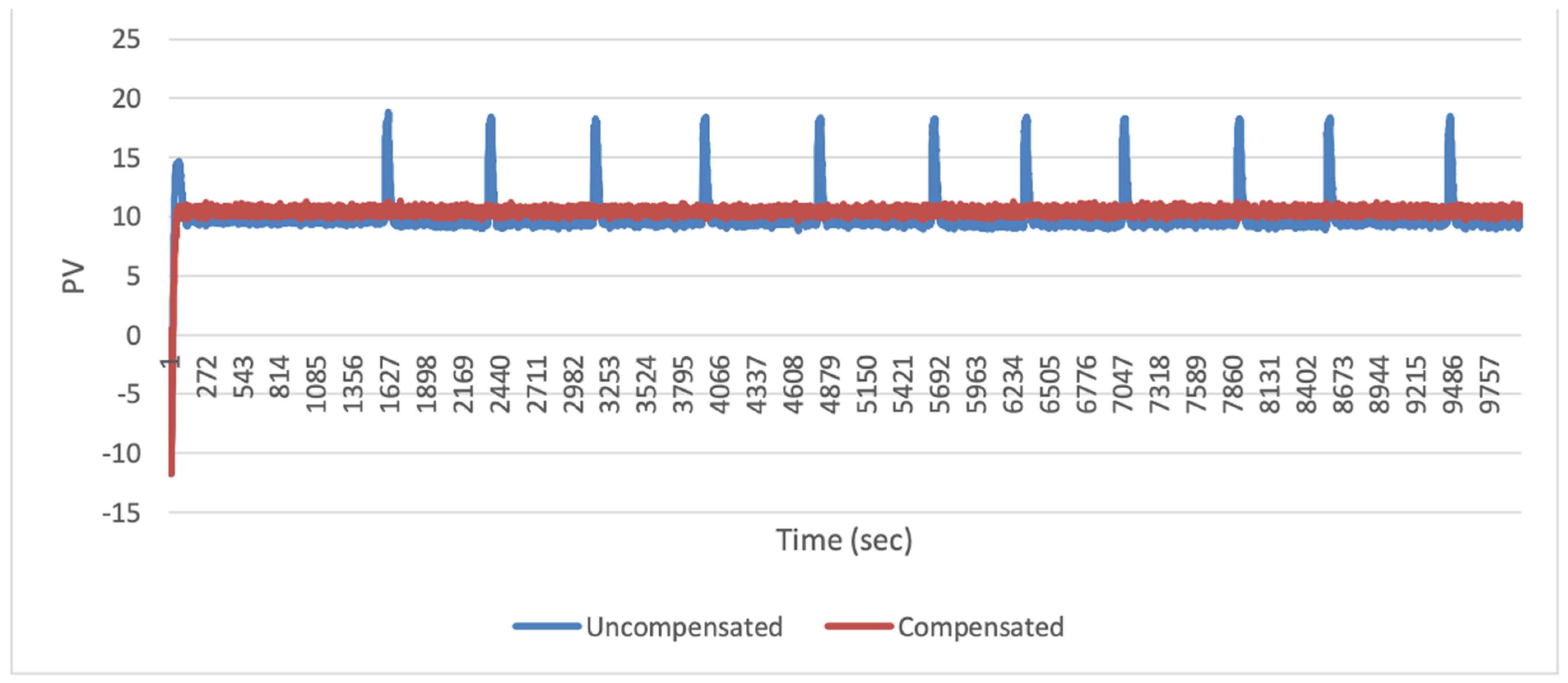
Figure 7.
Comparison between the three types of compensation methods (S=5, J=1).
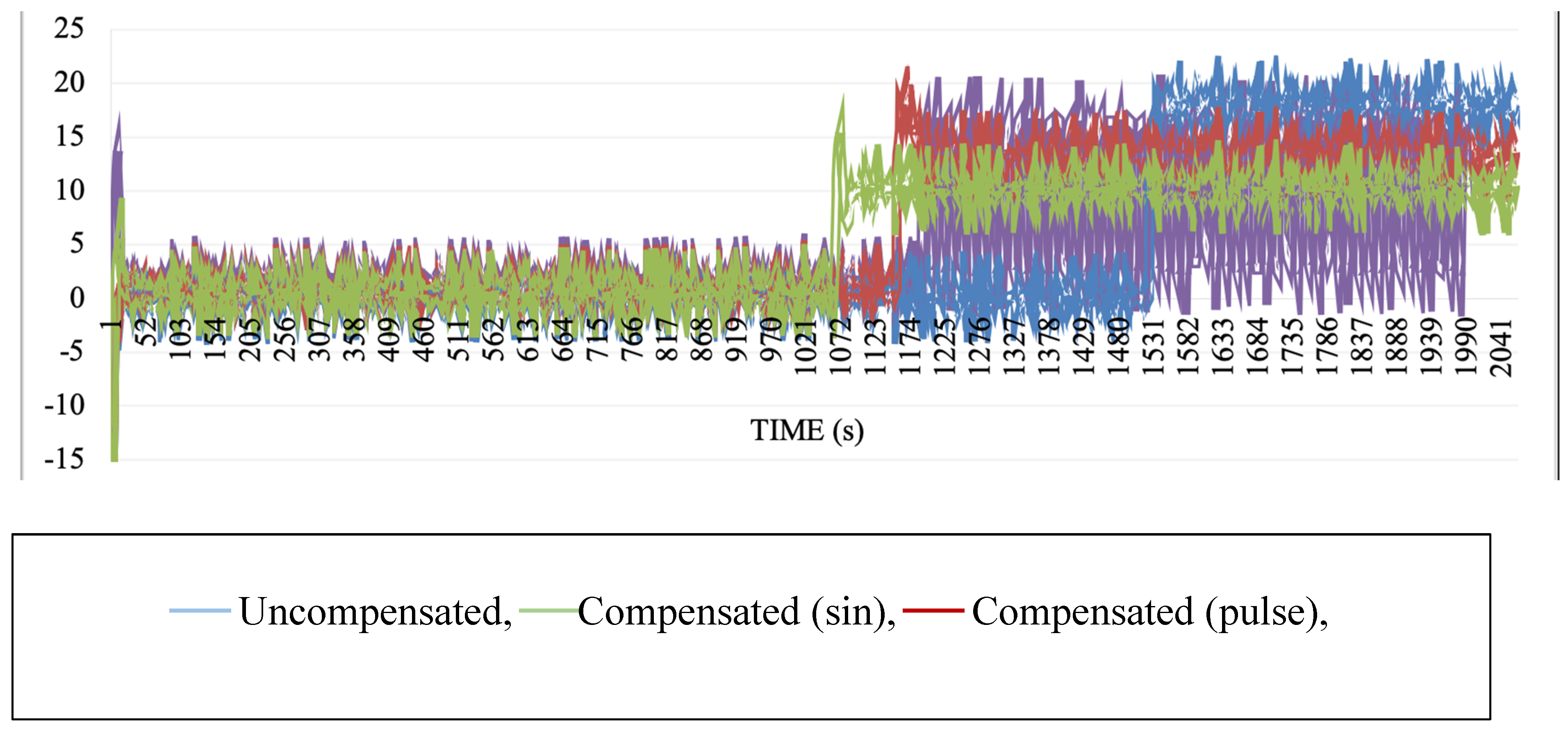
Figure 8.
Comparison between the three types of compensation methods (S=1, J=1).
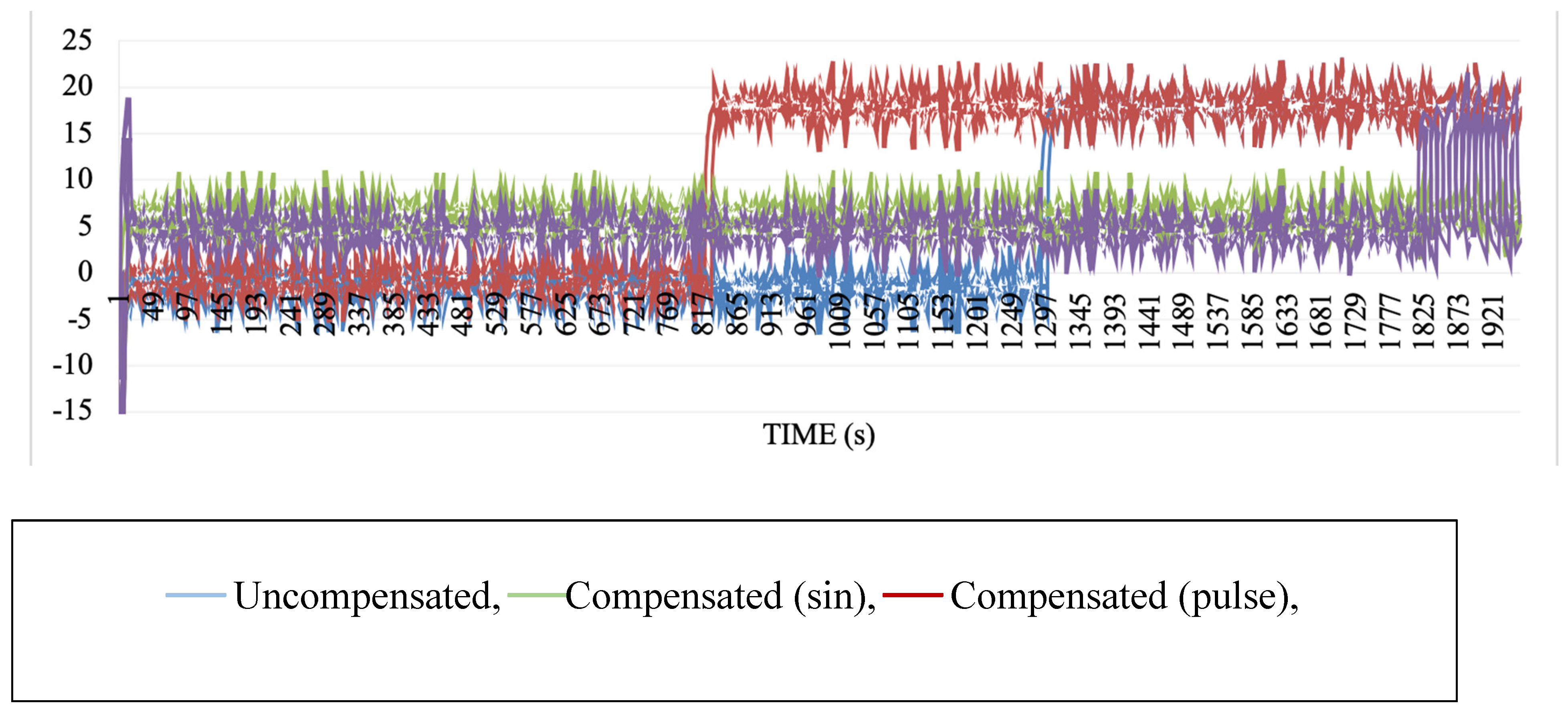
Figure 9.
Comparison between many various levels of stiction on the sinusoidal compensation method.
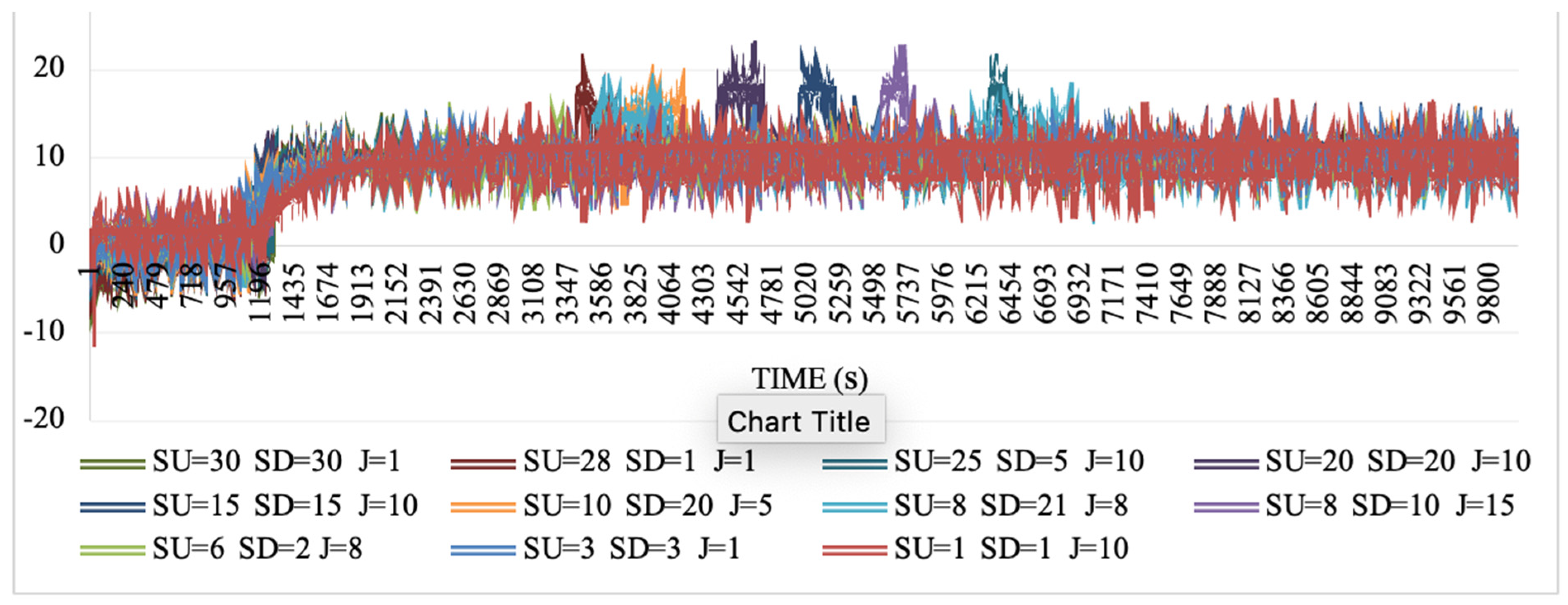
Figure 10 demonstrates the ability of sinusoidal compensation to reduce the integral squared error (ISE) across varying stiction severities. These results highlight a significant improvement compared to baseline control (no compensation). For mild stiction, the method achieved a 50% reduction in ISE, proving its effectiveness in stabilizing the control system with minimal intervention. For moderate and severe stiction, reductions of 65% and 75%, respectively, showcase the robustness of the sinusoidal approach, even in challenging conditions. This illustrates its potential to enhance precision and process control.
In Figure 11, the energy consumption of sinusoidal compensation is compared to that of pulse-based methods. The sinusoidal method reduced energy use by up to 30%, thanks to smoother valve movements and diminished oscillations. By eliminating the aggressive valve dynamics typical of pulse-based methods, sinusoidal compensation not only saves energy but also lowers operational costs. This energy efficiency aligns with sustainability goals, offering an eco-friendly solution for industrial applications.
Figure 12 presents trends in maintenance costs associated with control valves over time, comparing systems with and without sinusoidal compensation. The sinusoidal method significantly reduced maintenance expenses by minimizing valve wear through smoother and less aggressive operations, extending equipment lifespan. This reduction in maintenance costs is especially impactful in high-wear environments, providing long-term economic and operational benefits. Additionally, reduced maintenance downtime enhances overall manufacturing productivity.
These findings are further supported by data on valve travel distance, showing reduced maintenance wear and lower power consumption, as detailed in Table 5.
5. Conclusions
In conclusion, three compensation methods were used to reduce valve stiction. Despite that the Kc and τi tuning method seems the easiest to apply however it causes long settling times, or due to low Kc values, instability is cause. With the two suitable options between the sinusoidal and pulse method, sinusoidal was found to be superior showing the lowest error ranging from 0.8 to 2 in most cases. The sinusoidal compensation method offers a promising solution for enhancing the sustainability of manufacturing enterprises. Its ability to minimize oscillations and optimize energy usage ensures better operational efficiency and reduced environmental impact. By significantly reducing oscillations in the process variable, the method enhances system stability and operational efficiency. This improvement is critical for maintaining consistent product quality, especially in manufacturing environments where precision is paramount.
The method’s ability to achieve faster rise times and shorter settling times underscores its impact on improving system responsiveness. With a reduction in integral square error (ISE) values by 50% for mild stiction and up to 75% for moderate to severe stiction, the sinusoidal compensation approach exhibits superior performance compared to baseline and alternative methods. This makes it particularly suitable for high-stiction scenarios where other methods, such as pulse-based compensation or PID tuning, fall short.
References
- Bascur, O. Process control and operational intelligence. In SME Mineral Processing and Extractive Metallurgy; 2019. [Google Scholar]
- Choudhury, M.A.A.S.; Shah, S.L.; Thornhill, N.F.; Rajapakse, A. Modelling and compensation of valve stiction. Journal of Process Control 2005, 15, 19–29. [Google Scholar]
- Daneshwar, M.A.; Noh, N.M. Identification of a process with control valve stiction using a fuzzy system: A data-driven approach. Journal of Process Control 2014. [Google Scholar] [CrossRef]
- de Wit, C.; Olsson, H.; Åström, K.J.; Lischinsky, P. A new model for control of systems with friction. IEEE Transactions on Automatic Control 1995, 40, 419–425. [Google Scholar] [CrossRef]
- Di Capaci, R.B.; Scali, C. System identification applied to stiction quantification in industrial control loops. Journal of Process Control 2016. [Google Scholar] [CrossRef]
- Di Capaci, R.B.; Scali, C.; Vallati, C.; Anastasi, G. A technological demonstrator for cloud-based performance monitoring and assessment of industrial plants. IFAC-PapersOnLine.
- Farenzena, B.M.; Trierweiler, J.O. Stiction compensation in control valves: A comparison of techniques. Control Engineering Practice 2007, 15, 431–441. [Google Scholar]
- Garrido, J.; Ruz, M.; Jiménez, J. Stiction compensation for low-cost electric valves. Control Engineering Practice 2023. [Google Scholar]
- Hagglund, T. A friction compensator for pneumatic control valves. Control Engineering Practice 2002, 10, 1133–1142. [Google Scholar] [CrossRef]
- Hassan, M.A.M. Industrial Pneumatic Valve Stiction Compensation [ProQuest Dissertations & Theses]. 2015. Available online: https://www.proquest.
- Horch, A. Advanced control valve stiction modeling for industrial applications. Journal of Process Control 2000, 10, 103–112. [Google Scholar]
- Horch, A.; Isaksson, A.J. A method for detection of stiction in control valves. IFAC Proceedings Volumes 1998. [Google Scholar] [CrossRef]
- Kano, M.; Maruta, H. Practical model and detection algorithm for valve stiction. IFAC Proceedings Volumes 2004. [Google Scholar] [CrossRef]
- Lakshminarayanan, S. A new unified approach to valve stiction quantification and compensation. Industrial & Engineering Chemistry Research 2009. [Google Scholar]
- Mathur, N.; Asirvadam, V.S.; Aziz, A.A. Control Valve Life Cycle Prediction. IEEE Conferences 2020. [Google Scholar]
- Navada, B.R.; Sravani, V. Enhancing Industrial Valve Diagnostics. Applied System Innovation 2024. [Google Scholar] [CrossRef]
- Ruel, M. Understanding stiction in process control valves. Instrumentation and Control Systems 2000, 73, 63–66. [Google Scholar]
- Srinivasan, R.; Rengaswamy, R. Approaches for efficient stiction compensation. Computers & Chemical Engineering 2008. [Google Scholar]
- Vallati, C.; Anastasi, G. Techniques of analysis of valve stiction: From modeling to diagnostics. Industrial Engineering Chemistry Research 2020. [Google Scholar]
- Wu, X.; Wang, M.; Liao, P.; Shen, J.; Li, Y. Post-combustion CO2 capture for power plants: A critical review and perspective. Applied Energy 2020, 269, 114910. [Google Scholar]
Figure 1.
Typical input-output characteristic of a sticky valve (Choudhury et al., 2005).
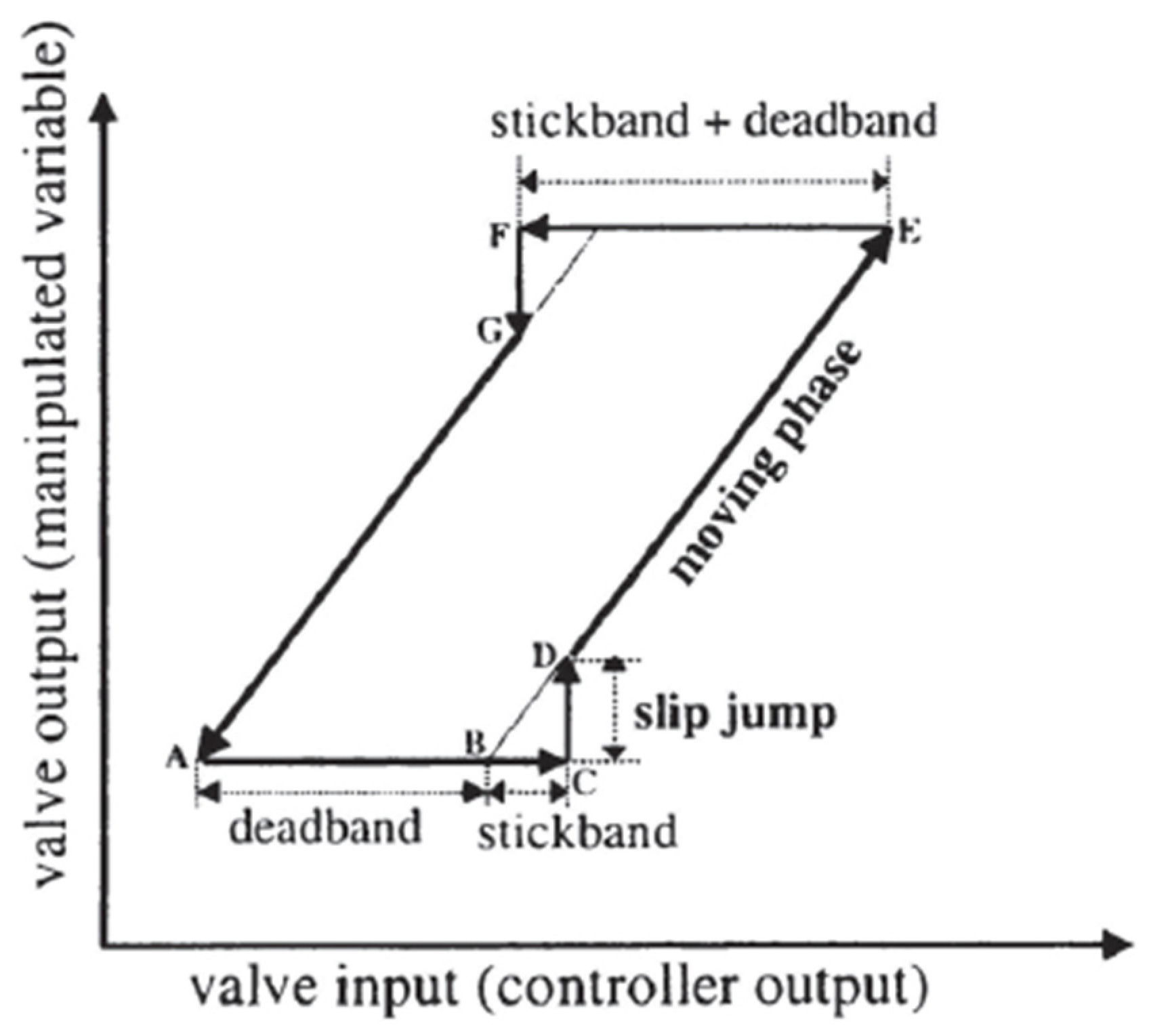
Figure 2.
Choudhury’s model plus compensator (Choudhury et al., 2005).
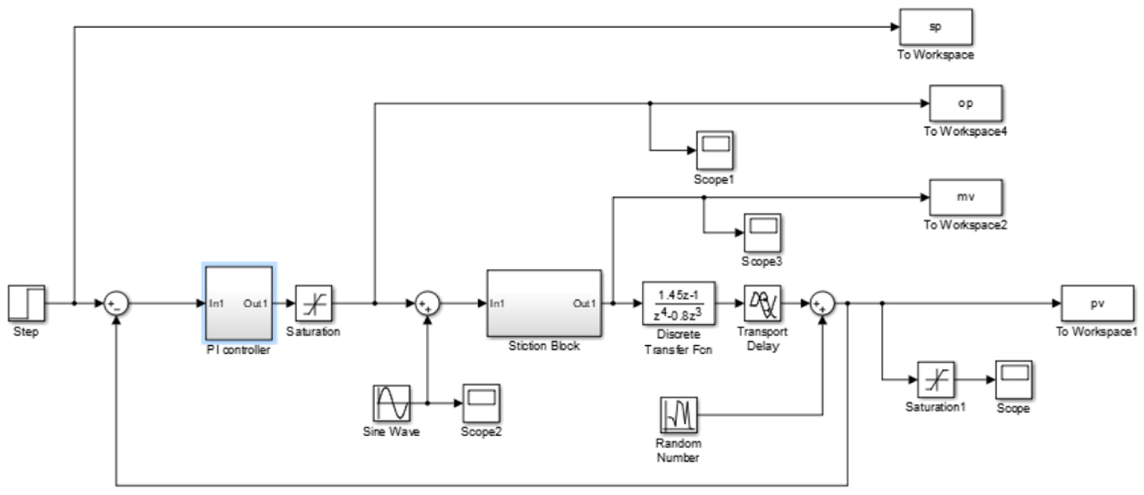
Figure 3.
Modified version of two-parameter data-driven stiction model.
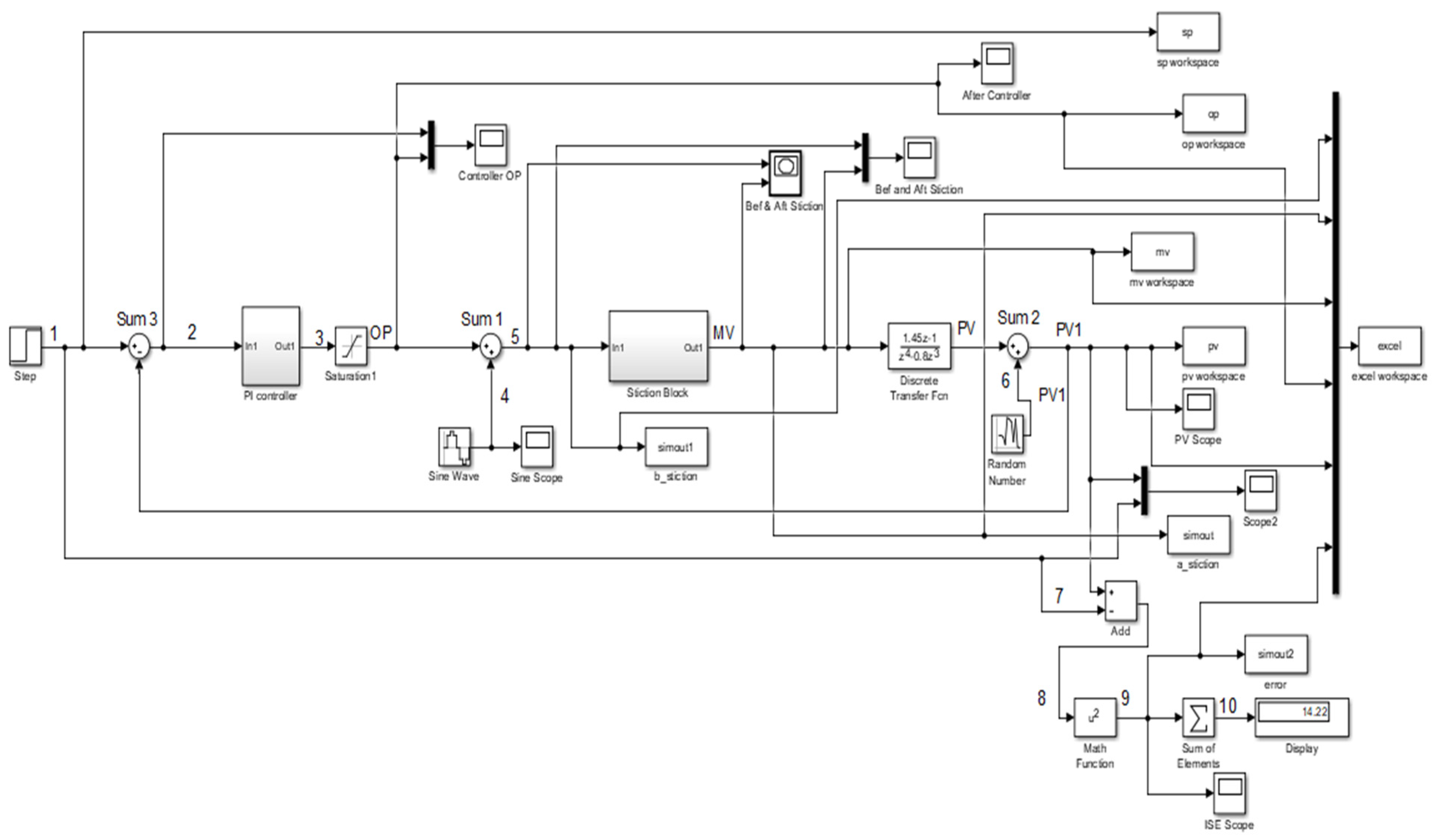
Figure 4.
DoE Plot to identify the effect of each variable on the output.
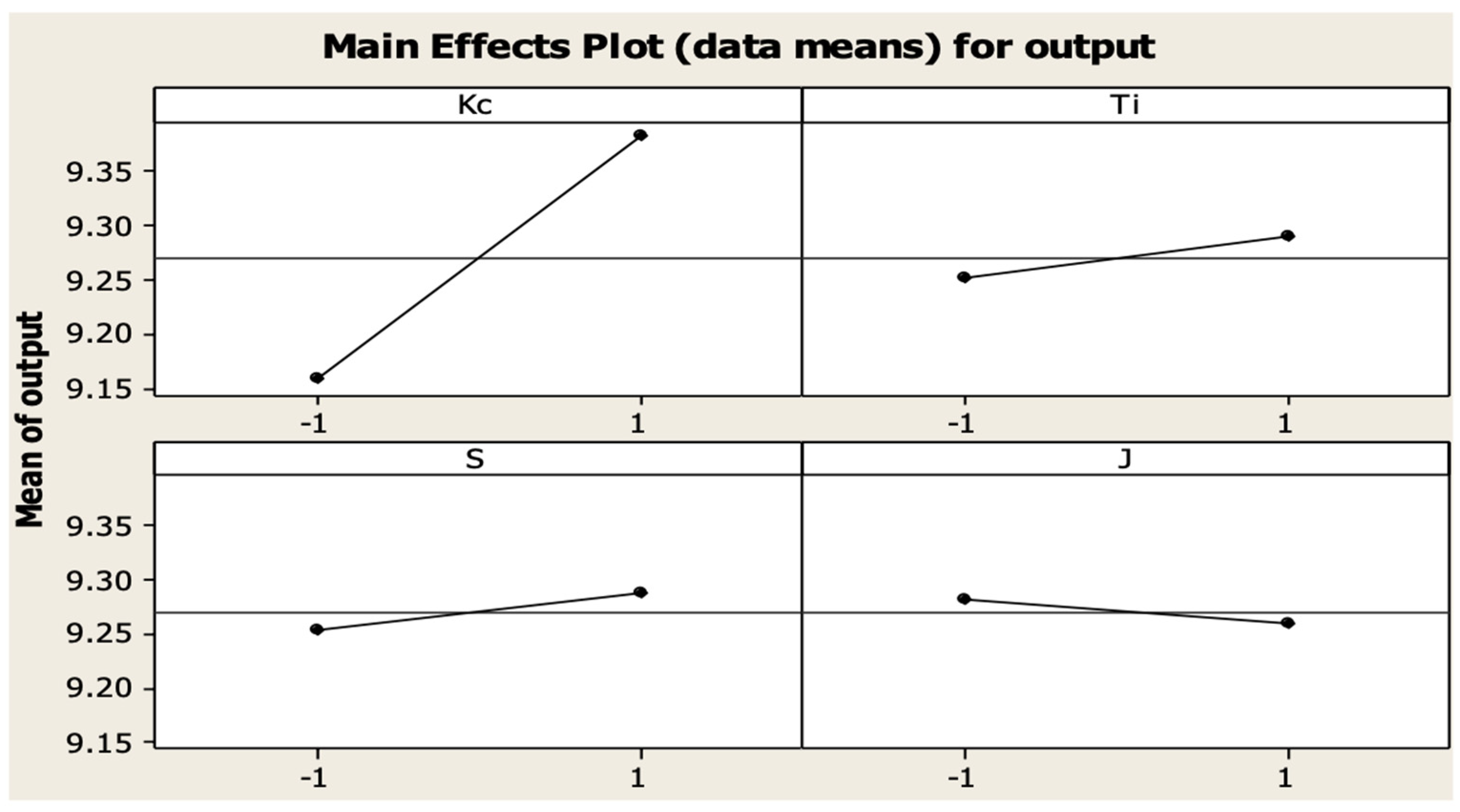
Figure 5.
Interaction Plot of the Output.
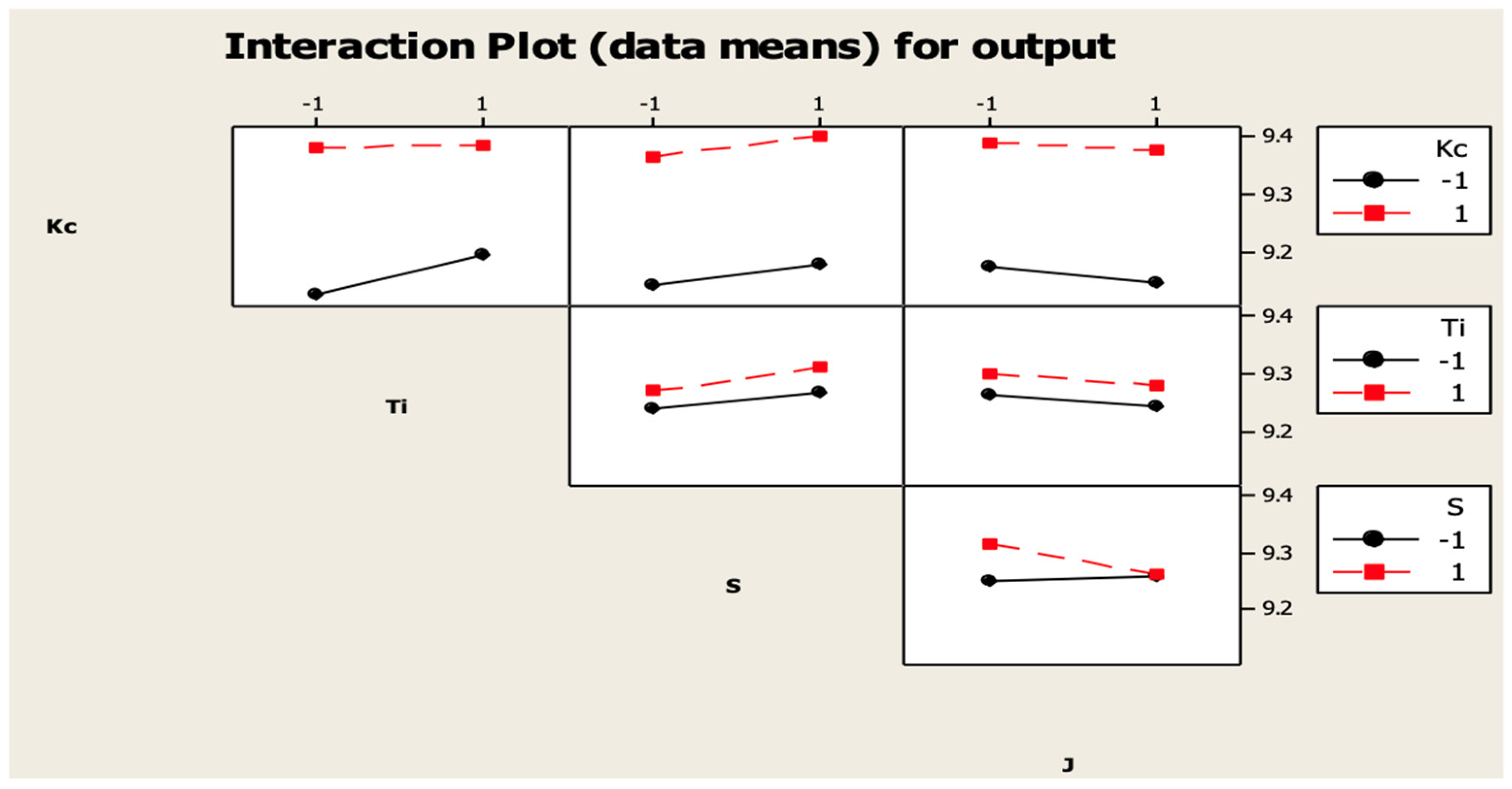
Figure 10.
Graph comparing ISE values across different stiction severities with and without sinusoidal compensation.
Figure 10.
Graph comparing ISE values across different stiction severities with and without sinusoidal compensation.
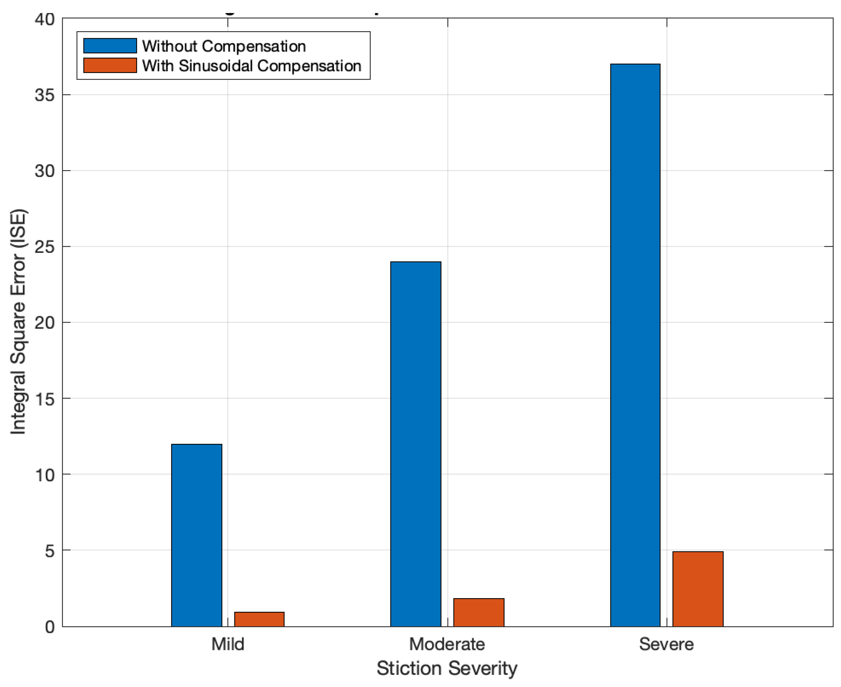
Figure 11.
Energy consumption analysis of sinusoidal versus pulse-based methods.
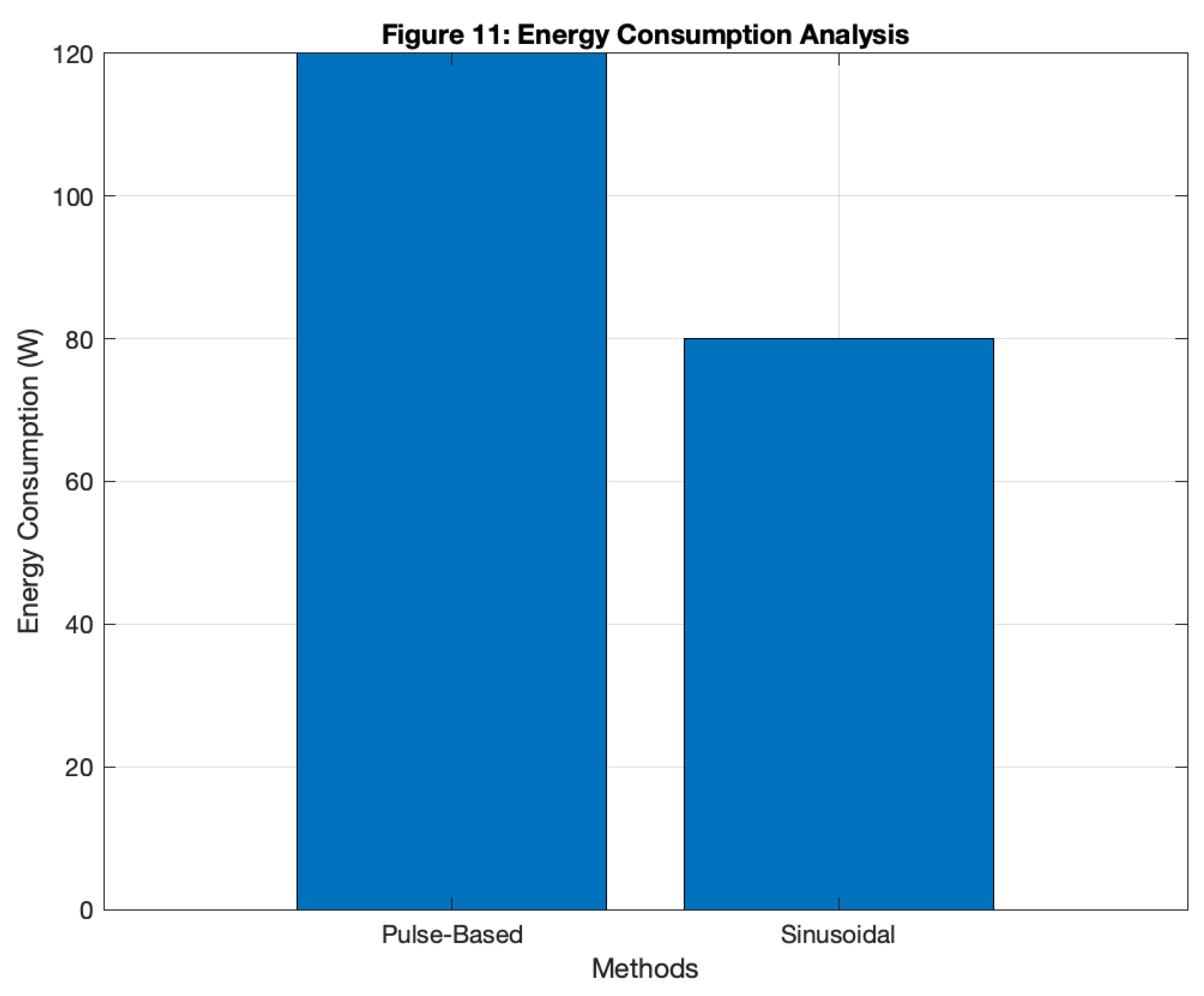
Figure 12.
Maintenance cost trends showing reduced wear and extended valve lifespan with sinusoidal compensation.
Figure 12.
Maintenance cost trends showing reduced wear and extended valve lifespan with sinusoidal compensation.
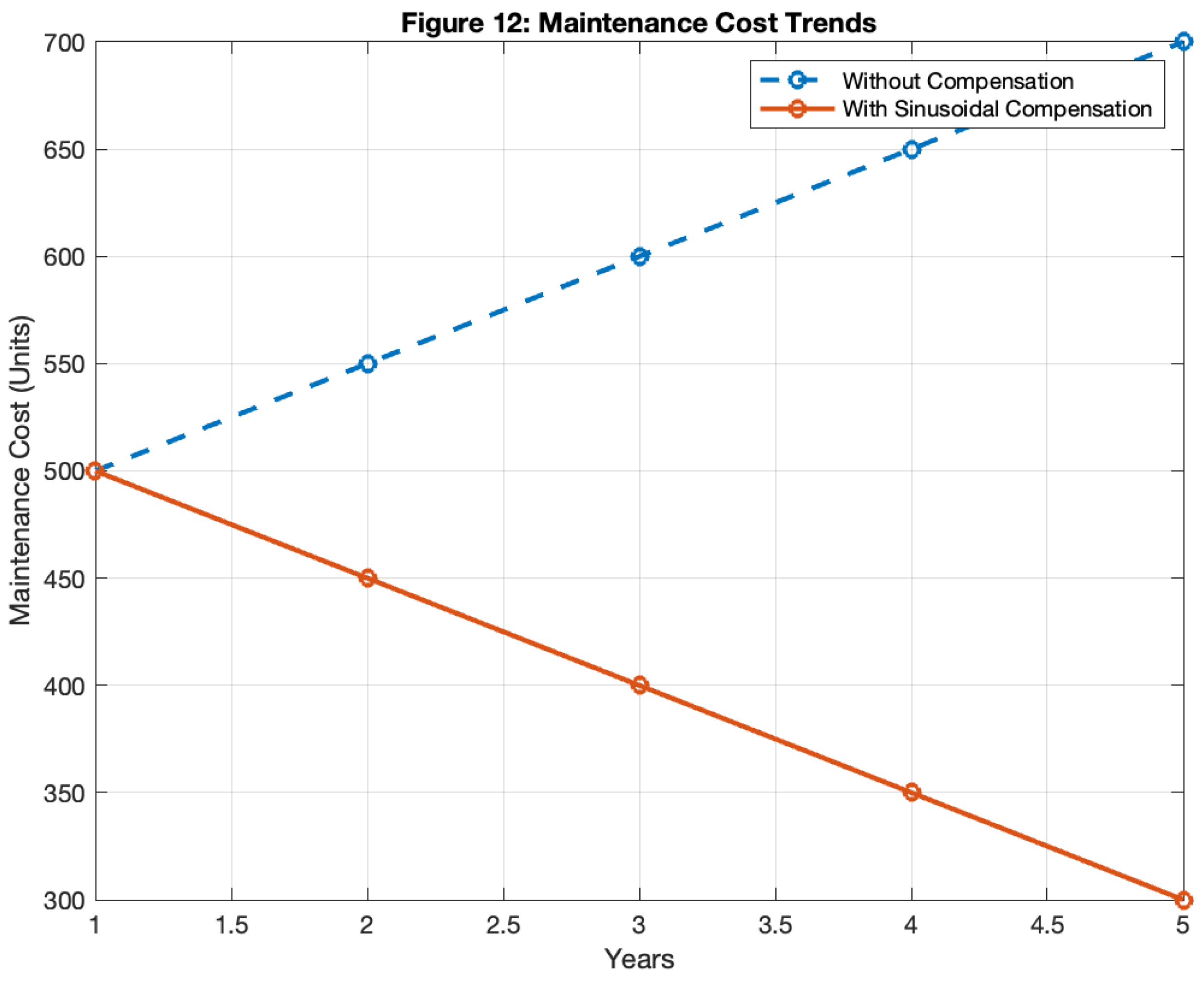
Table 3.
Quantification of the Stiction.
| Stiction Parameters | Classification | ||||
| S | J | Area | High stiction | Mild stiction | Low stiction |
| 1 | 0 | 39.919 | ✓ | ||
| 1 | 1 | 0.628 | ✓ | ||
| 5 | 0 | 43.263 | ✓ | ||
| 5 | 1 | 36.789 | ✓ | ||
| 10 | 0 | 57.14 | ✓ | ||
| 10 | 1 | 45.22 | ✓ | ||
Table 4.
Tuning control parameter for every experiment.
| S | J | Kc | τi |
| 1 | 0 | 0.09595 | 0.1 |
| 1 | 1 | 0.0899 | 0.1 |
| 5 | 0 | 0.1 | 0.1 |
| 5 | 1 | 0.1 | 0.1 |
| 10 | 0 | 0.105 | 0.1 |
| 10 | 1 | 0.1055 | 0.1 |
Table 5.
Metric measurement with and without compensation.
| Metric | Without Compensation | With Compensation |
| Valve Travel Distance (DD) | 0.29 m | 0.14 m |
| Power Requirement (PP) | 120.01 W | 90.005 W |
| Energy Consumption (EE) | 432.04 kWh | 324.02 kWh |
| Maintenance Wear (WW) | 52.2 units | 25.2 units |
| Repair Frequency (RR) | 1.04 repairs | 0.504 repairs |
Disclaimer/Publisher’s Note: The statements, opinions and data contained in all publications are solely those of the individual author(s) and contributor(s) and not of MDPI and/or the editor(s). MDPI and/or the editor(s) disclaim responsibility for any injury to people or property resulting from any ideas, methods, instructions or products referred to in the content. |
© 2025 by the authors. Licensee MDPI, Basel, Switzerland. This article is an open access article distributed under the terms and conditions of the Creative Commons Attribution (CC BY) license (http://creativecommons.org/licenses/by/4.0/).
Copyright: This open access article is published under a Creative Commons CC BY 4.0 license, which permit the free download, distribution, and reuse, provided that the author and preprint are cited in any reuse.


